Energy of Isolated Systems at Retarded Times as the
Null Limit of Quasilocal Energy

Abstract

We define the energy of a perfectly isolated system at a given retarded time as the suitable null limit of the quasilocal energy $E$. The result coincides with the Bondi-Sachs mass. Our $E$ is the lapse-unity shift-zero boundary value of the gravitational Hamiltonian appropriate for the partial system $\Sigma$ contained within a finite topologically spherical boundary $B=\partial\Sigma$. Moreover, we show that with an arbitrary lapse and zero shift the same null limit of the Hamiltonian defines a physically meaningful element in the space dual to supertranslations. This result is specialized to yield an expression for the full Bondi-Sachs four-momentum in terms of Hamiltonian values.

Introduction

To define quasilocal energy in general relativity, one can begin with a suitable action functional for the time history ${\cal M}$ of a spatially bounded system $\Sigma$. Here “suitable” means that in the associated variational principle the induced metric on the time history ${\cal T}$ of the system boundary $B=\partial\Sigma$ is fixed. In particular, this means that the lapse of proper time between the boundaries of the initial and final states of the system $\Sigma$ must be fixed as boundary data. The quasilocal energy (QLE) is then defined as minus the rate of change of the classical action (or Hamilton-Jacobi principal function) corresponding to a unit increase in proper time.[1, 2] So defined, the QLE is a functional on the gravitational phase space of $\Sigma$, and is the value of the gravitational Hamiltonian corresponding to unit lapse function and zero shift vector on the system boundary $B$. Although other definitions of quasilocal energy have been proposed (see, for example, the references listed in [1]), the QLE considered here has the key property, which we consider crucial, that it plays the role of internal energy in the thermodynamical description of coupled gravitational and matter fields.[3]

In this paper we define the energy of a perfectly isolated system at a given retarded time as the suitable limit of the quasilocal energy $E$ for the partial system enclosed within a finite topologically spherical boundary. For our choice of asymptotic reference frame the energy that we compute equals what is usually called the Bondi-Sachs mass.[5, 6] As we shall see, our asymptotic reference frame defines precisely that infinitesimal generator of the Bondi-Metzner-Sachs (bms) group corresponding to a pure time translation.[7, 6, 8] We also show that in the same null limit the lapse-arbitrary, shift-zero Hamiltonian boundary value defines a physically meaningful element in the space dual to supertranslations. This dual space element, it turns out, coincides with the “supermomentum” discussed by Geroch.[9] Our results are then specialized to an expression for the full Bondi-Sachs four-momentum in terms of Hamiltonian values. It is already known that when $B$ is the two-sphere at spacelike infinity, the quasilocal and Arnowitt-Deser-Misner[10] notions of energy-momentum agree.[1, 3] Our results therefore indicate that the quasilocal formalism provides a unified Hamiltonian framework for describing the standard notions of gravitational energy-momentum in asymptopia.

Before turning to the technical details, let us first present a short overview of our approach. Consider a spacetime ${\cal M}$ which is asymptotically flat at future null infinity ${\cal I}^{+}$ and a system $(w,R,\theta,\phi)$ of Bondi coordinates thereon.[6] The retarded time $w$ labels a one-parameter family of outgoing null hypersurfaces ${\cal N}(w)$. The coordinate $R$ is a luminosity parameter (areal radius) along the outgoing null-geodesic generators of the hypersurfaces ${\cal N}(w)$. The Bondi coordinate system also defines a two-parameter family of topologically spherical two-surfaces $B(w,R)$. It suits our purposes to consider only a single null hypersurface of the family ${\cal N}(w)$, say ${\cal N}(w_{*})$, the one determined by setting $w$ equal to an arbitrary constant $w_{*}$. The collection $B(w_{*},R)$ of two-surfaces foliates ${\cal N}(w_{*})$, and in the $R\to\infty$ limit these two-surfaces converge on an infinite-radius round sphere $B(w_{*},\infty)$. To streamline the presentation, we refer to our generic null hypersurface simply as $\cal N$; and we use the plain letter $B$ to denote both the $\cal N$-foliating collection $B(w_{*},R)$ and a single generic two-surface of this collection. Now, should we desire a more general ${\cal N}$-foliating collection of two-surfaces, we could, of course, introduce a new radial coordinate $\bar{R}$. For a fixed retarded time $w=w_{*}$ the new two-surfaces would then arise as level surfaces of constant $\bar{R}$. However, we shall not consider such a new radial coordinate, because the new two-surfaces would not necessarily converge towards a round sphere in the asymptotic limit. At any rate, we could handle such an additional kinematical freedom, were it present, by assuming that along each outgoing null ray $\bar{R}$ approached $R$ at a sufficiently fast rate in the asymptotic limit.

Our first goal is to compute the QLE within a two-surface $B$ in the limit as $B$ approaches a spherical cut of ${\cal I}^{+}$ along the null surface $\cal N$, and to show that this result coincides with the Bondi-Sachs mass:

$$M_{{}_{BS}}(w_{*})=\lim_{R\rightarrow\infty}\int_{B(w_{*},R)}{\rm d}^{2}x\sqrt{\sigma}\varepsilon\,.$$ (1)

Here $\varepsilon=(k-k|^{\scriptscriptstyle{\rm ref}})/\kappa$ is the quasilocal energy surface density with $\kappa=8\pi$ (in geometrical units) and $\sigma$ is the determinant of the induced metric on $B$. Recall that $k$ denotes the mean curvature of $B$ as embedded in some spacelike spanning three-surface $\Sigma$. Since both $B$ and $\Sigma$ are embedded in the physical spacetime ${\cal M}$, we sometimes use the notation $\varepsilon|^{\scriptscriptstyle{\rm phy}}=k/\kappa$. Also recall that $k|^{\scriptscriptstyle{\rm ref}}$ denotes the mean curvature of a surface which is isometric to $B$ but which is embedded in a three-dimensional reference space different than $\Sigma$. Here we choose the reference space to be flat Euclidean space $E^{3}$, i. e. we assign a flat three-slice of Minkowski spacetime the zero value of energy.[1] Although a definition of the zero-energy reference in terms of flat space is neither always essential nor appropriate[11], it is the correct choice for the analysis of this paper.

In order to define $k$, we must select such a three-surface spanning $B$ for each $R$ value. (For a single $B$ many different spanning three-surfaces will determine the same $k$. In fact, $k$ is determined solely by $B$ and a timelike unit vector field $u^{\mu}$ on $B$, which can be considered as the unit normal of a slice $\Sigma$. Thus, the continuation of $\Sigma$ away from $B$ is not needed; moreover, such a continuation of $\Sigma$ might not be defined throughout the interior of ${\cal M}$. Therefore, though we speak of choosing a $\Sigma$ three-surface to span $B$ for each $R$ value, we are really fixing only a timelike unit normal vector field at $B$.) For generality, we leave the choice of spanning three-surface $\Sigma$ essentially arbitrary at each $R$ value, but we do enforce a definite choice asymptotically. Heuristically, as $R\rightarrow\infty$ the $\Sigma$ three-surface spanning $B$ approaches an asymptotic three-surface $\Sigma_{\infty}$ which spans a round infinite-radius spherical cut of ${\cal I}^{+}$ (see the figure). Our construction is, as expected, sensitive to the choice of asymptotic three-surface $\Sigma_{\infty}$. Said another way, the QLE depends on the fleet of observers at $B$ whose four-velocities are orthogonal to the spanning three-surface at $B$. Therefore, one expects a priori the expression on the right-hand side of (1) to depend on the choice of asymptotic fleet associated with the two-sphere at ${\cal I}^{+}$. The asymptotic fleet we choose corresponds to a pure bms time translation: each member of the asymptotic fleet rides along $\partial/\partial w$. Note that, although $\partial/\partial w$ is everywhere timelike in ${\cal M}$ (at least in the relevant exterior regions), the extension of $\partial/\partial w$ to ${\cal I}^{+}$ in a conformal completion $\hat{\cal M}$ of the physical spacetime ${\cal M}$ is in fact a null vector which lies in ${\cal I}^{+}$. (While we occasionally find it clarifying to make reference to the concept of a conformal completion, we do not explicitly use conformal completions in this paper.) Therefore, heuristically, one should envision $\Sigma_{\infty}$ as a spacelike slice which becomes null asymptotically (see the figure).

This paper is organized as follows. In a preliminary section we write down the familiar Bondi-Sachs form[7, 12] of the spacetime metric as well as asymptotic expansions for the associated metric coefficients. We also introduce on $\cal M$ two future-pointing null vector fields $k^{\mu}$ and $l^{\mu}$ (do not confuse $k^{\mu}$ with the mean curvature $k$). Both vector fields point everywhere normal to our collection $B(w,R)$ of two-surfaces, and $k_{\mu}l^{\mu}=-1$. Next, we construct on ${\cal N}$ a timelike vector field $u^{\mu}:=\frac{1}{2}k^{\mu}+l^{\mu}$ (equality restricted to ${\cal N}$), which in our analysis will define for each $B$ along $\cal N$ a spacelike spanning three-surface $\Sigma$. In $\S$II we use the $\Sigma$ three-surfaces determined by $u^{\mu}$ to define an unreferenced energy surface density $\varepsilon|^{\scriptscriptstyle{\rm phy}}=k/\kappa$ for each $B$ slice of $\cal N$ and then examine the asymptotic limit of $k/\kappa$. In $\S$III we consider the asymptotic expression for the flat-space reference density $\varepsilon|^{\scriptscriptstyle{\rm ref}}=k|^{\scriptscriptstyle{\rm ref}}/\kappa$, but give the derivation of this expression in the Appendix. Next, we assemble the results of the previous two sections and prove the main claim (1). In $\S$IV we examine the “smeared energy surface density,” which is the Hamiltonian value corresponding to an arbitrary supertranslation. We then specialize our result for the smeared energy surface density to express the full Bondi-Sachs four-momentum in terms of Hamiltonian values. In $\S$V we examine the smeared energy surface density via the spin-coefficient formalism, and show that it equals the “supermomentum” of Geroch[9] as written by Dray and Streubel.[13] The Appendix is devoted to a detailed analysis of the reference term.

I Preliminaries

In terms of a Bondi coordinate system the metric of our asymptotically flat spacetime ${\cal M}$ takes the standard form[7, 12]

$$g_{\mu\nu}{\rm d}x^{\mu}{\rm d}x^{\nu}=-UV{\rm d}w^{2}-2U{\rm d}w{\rm d}R+\sigma_{ab}({\rm d}x^{a}+W^{a}{\rm d}w)({\rm d}x^{b}+W^{b}{\rm d}w){\,},$$ (2)

where $a,b$ are $B$ indices running over $\theta,\phi$. We assume the following expansions for the various metric coefficients above:

$$V = 1-2{\rm m}R^{-1}+\Delta_{V}$$ ()

$$U = 1-{\textstyle\frac{1}{2}}(X^{2}+Y^{2})R^{-2}+\Delta_{U}$$ ()

$$W^{\theta} = (2X\cot\theta+X_{,\theta}+Y_{,\phi}\csc\theta)R^{-2}+\Delta_{W^{\theta}}$$ (3)

$$W^{\phi} = \csc\theta\left(2Y\cot\theta+Y_{,\theta}-X_{,\phi}\csc\theta\right)R^{-2}+\Delta_{W^{\phi}}$$ ()

$$\sigma_{ab} = R^{2}\delta_{ab}+\left[(2X)\theta_{,a}\theta_{,b}+(4Y\sin\theta)\theta_{,(a}\phi_{,b)}-(2X\sin^{2}\theta)\phi_{,a}\phi_{,b}\right]R+\Delta_{\sigma_{ab}}{\,}.$$ ()

Here $X(w,\theta,\phi)$ and $Y(w,\theta,\phi)$ are respectively the real and imaginary parts of the asymptotic shear $c=X+{\rm i}Y$, ${\rm m}(w,\theta,\phi)$ is the all-important mass aspect, $\delta_{ab}$ is the metric of a unit-radius round sphere, and commas denote partial differentiation. In the Appendix we examine the form of the two metric $\sigma_{ab}$ in more detail. Remainder terms, denoted by the $\Delta$ symbol, always fall off faster (or have slower growth, as the case may be) than the terms which precede them. For instance, $\Delta_{V}$ denotes a term which falls off faster than $O(R^{-1})$.

Introduce the future-directed null covector field $k_{\mu}=-e^{\eta}\nabla_{\mu}w$, where the scalar function $\eta=\eta(w,R,\theta,\phi)$ is a point-dependent boost parameter. The null covector $k_{\mu}$ is orthogonal to the spheres $B(w,R)$, and the function $\eta$ gives us complete freedom in choosing the extent of $k_{\mu}$ at each point of any $B$ two-surface. We shall find it necessary later to assume that $\eta$ falls off faster than $1/\sqrt{R}$ on every outgoing ray. Also define another future-directed null vector field $l^{\mu}$ which is orthogonal to the $B(w,R)$ and normalized so that $k_{\mu}l^{\mu}=-1$. As one-forms these null normals are

$$k_{\mu}{\rm d}x^{\mu} = -e^{\eta}{\rm d}w$$ ()

$$l_{\mu}{\rm d}x^{\mu} = -e^{-\eta}U{\rm d}R-{\textstyle\frac{1}{2}}e^{-\eta}UV{\rm d}w\,,$$ ()

while as vector fields they are

$$k^{\mu}\partial/\partial x^{\mu} = e^{\eta}U^{-1}\partial/\partial R$$ ()

$$l^{\mu}\partial/\partial x^{\mu} = e^{-\eta}\partial/\partial w-{\textstyle\frac{1}{2}}e^{-\eta}V\partial/\partial R-e^{-\eta}W^{a}\partial/\partial x^{a}\,.$$ ()

Now define $u^{\mu}:=\frac{1}{2}k^{\mu}+l^{\mu}$ and $n^{\mu}:=\frac{1}{2}k^{\mu}-l^{\mu}$ along ${\cal N}$ as the timelike and spacelike unit normals of the $B$ two-surfaces. For each slice $B$ of the null hypersurface ${\cal N}$, the normals $u^{\mu}$ and $n^{\mu}$ determine a spanning spacelike three-surface $\Sigma$. As mentioned previously, the three-surface $\Sigma$ is not unique and, moreover, need not be defined throughout ${\cal M}$. Indeed, there is no guarantee that $u^{\mu}$ as defined is even surface-forming. (That is, in general $u_{\mu}$ does not satisfy the Fröbinius condition $u_{[\alpha}\nabla_{\mu}u_{\nu]}=0$.) Nevertheless, our construction provides us with what we need: a unit timelike vector $u^{\mu}$ orthogonal to $B$. We can therefore obtain an unreferenced energy surface density $k/\kappa$ which is the same for any slice or partial slice $\Sigma$ that contains $B$ and has timelike unit normal which agrees with $u^{\mu}$ at $B$.

Our construction implies

$$u^{\mu}\partial/\partial x^{\mu}\rightarrow\partial/\partial w$$ (7)

on each ray as $R\rightarrow\infty$. Now, the standard realization of the bms-group Lie algebra (as vector fields on future null infinity) identifies the extension of $\partial/\partial w$ to ${\cal I}^{+}$ (in a conformal completion $\hat{\cal M}$ of ${\cal M}$) with a pure time translation.[7, 6] Therefore, asymptotically, our fiducial surface $\Sigma_{\infty}$ determines precisely the pure time-translation generator of the bms group. We do not claim that $u^{\mu}$ generates an “infinitesimal asymptotic symmetry transformation” in the sense of Sachs[7], i. e. that the various coefficients associated with the transformed metric $g_{\mu\nu}+2\nabla_{(\mu}u_{\nu)}$ satisfy the fall-off conditions (() ‣ I); however, this is unimportant for our construction.

II Computation of the quasilocal energy surface density

We now turn to the task of calculating an expression for the unreferenced quasilocal energy surface density $\varepsilon|^{\scriptscriptstyle{\rm phy}}=k/\kappa$. Our starting point is the definition $k:=-\sigma^{\mu\nu}\nabla_{\mu}n_{\nu}$, where the two-metric $\sigma^{\mu\nu}=g^{\mu\nu}+2k^{(\mu}l^{\nu)}$ serves as the projection operator into $B$. We find it convenient to write $k=2\mu+\rho$, where in the standard notation of the spin-coefficient formalism[8] $-\mu$ and $\rho$ are, respectively, the expansions associated with the inward null normal and outward null normal to $B$. These are given by the formulae

$$\mu = {\textstyle\frac{1}{2}}\sigma^{\mu\lambda}\nabla_{\mu}l_{\lambda}={\textstyle\frac{1}{2}}(\nabla_{\mu}l^{\mu}+k^{\nu}l^{\mu}\nabla_{\mu}l_{\nu})$$ ()

$$\rho = -{\textstyle\frac{1}{2}}\sigma^{\mu\lambda}\nabla_{\mu}k_{\lambda}=-{\textstyle\frac{1}{2}}(\nabla_{\mu}k^{\mu}+l^{\nu}k^{\mu}\nabla_{\mu}k_{\nu})\,.$$ ()

As a technical tool, it proves convenient to introduce fiducial vector fields $\hat{k}^{\mu}$ and $\hat{l}^{\mu}$ determined from (() ‣ I) by setting $\eta=0$ on $\cal N$. From the middle expressions above, it is obvious that $\mu=e^{-\eta}\hat{\mu}$ and $\rho=e^{\eta}\hat{\rho}$, where the easier-to-calculate expressions $\hat{\mu}$ and $\hat{\rho}$ are built exactly as in (() ‣ II) but with the fiducial null normals $\hat{k}^{\mu}$ and $\hat{l}^{\mu}$. Therefore, we may assume that $\eta=0$ while calculating the spin coefficients in (() ‣ II) and then simply multiply the $\eta=0$ results by the appropriate factor to get the correct general expressions. Let us sketch the calculation. First, from (() ‣ Ia) with $\eta=0$ note that $\hat{k}^{\mu}\nabla_{\mu}\hat{k}_{\nu}=0$, because $\hat{k}_{\nu}$ is a gradient. Next, using both expressions (() ‣ I) with $\eta=0$, one can work the second term inside the parenthesis of (() ‣ IIa) into the form $\hat{k}^{\nu}\hat{l}^{\mu}\nabla_{\mu}\hat{l}_{\nu}=-U^{-1}\hat{l}^{\mu}\nabla_{\mu}U+\frac{1}{2}U\hat{k}^{\mu}\nabla_{\mu}V$. Finally, one writes the covariant-divergence terms as ordinary divergences; for example, $\nabla_{\mu}\hat{k}^{\mu}=(-g)^{-1/2}\partial_{\mu}(\sqrt{-g}\hat{k}^{\mu})$, where the square root of (minus) the determinant of the spacetime metric is $\sqrt{-g}=U\sqrt{\sigma}$.

Following these steps and multiplying by the appropriate boost factors at the end of the calculation, one finds

$$\mu = {\textstyle\frac{1}{4}}e^{-\eta}\sigma^{-1}\dot{\sigma}-{\textstyle\frac{1}{8}}e^{-\eta}V\sigma^{-1}\sigma^{\prime}-{\textstyle\frac{1}{2}}e^{-\eta}\delta_{a}W^{a}$$ ()

$$\rho = -{\textstyle\frac{1}{4}}e^{\eta}U^{-1}\sigma^{-1}\sigma^{\prime}{\,}.$$ ()

Here the over-dot denotes partial differentiation by $\partial/\partial w$, the prime denotes partial differentiation by $\partial/\partial R$, and $\delta_{a}$ denotes the $B$ covariant derivative. Since $R$ is an areal radius, we may take $\sigma=R^{4}\sin^{2}\theta$ [see the form of the $B$ metric given in (42)]. Therefore, we obtain the compact expressions

$$\mu = -{\textstyle\frac{1}{2}}e^{-\eta}VR^{-1}-{\textstyle\frac{1}{2}}e^{-\eta}\delta_{a}W^{a}$$ ()

$$\rho = -e^{\eta}U^{-1}R^{-1}\,.$$ ()

Adding twice (() ‣ IIa) to (() ‣ IIb), we arrive at our desired expression

$$k=-(e^{-\eta}V+e^{\eta}U^{-1})R^{-1}-e^{-\eta}\delta_{a}W^{a}\,,$$ (11)

which has the asymptotic form

$$k=-2R^{-1}+2{\rm m}(w_{*},\theta,\phi)R^{-2}-\delta_{a}W^{a}+\Delta_{k}\,.$$ (12)

Note that we have chosen not to expand the $O(R^{-2})$ pure divergence term $-\delta_{a}W^{a}$. Our assumption about the fall-off of $\eta$ ensures that a term $-\eta^{2}/R$ which appears in the asymptotic expression for $k$ can be swept into $\Delta_{k}$.

III The Bondi-Sachs mass

Write the total quasilocal energy as $E=E|^{\scriptscriptstyle{\rm phy}}-E|^{\scriptscriptstyle{\rm ref}}$, with the total unreferenced quasilocal energy $E|^{\scriptscriptstyle{\rm phy}}$ taken as

$$E|^{\scriptscriptstyle{\rm phy}}=\frac{1}{\kappa}\int_{B(w_{*},R)}{\rm d}^{2}x\sqrt{\sigma}k\,.$$ (13)

Plugging the expansion (12) into the above expression, using $\sqrt{\sigma}=R^{2}\sin\theta$ for our choice of coordinates, and integrating term-by-term, one finds

$$E|^{\scriptscriptstyle{\rm phy}}=-R+M_{{}_{BS}}(w_{*})+\Delta_{E|^{\scriptscriptstyle{\rm phy}}}\,.$$ (14)

Here the Bondi-Sachs mass associated with the $w=w_{*}$ cut of ${\cal I}^{+}$ is the two-surface average of the mass aspect evaluated at $w=w_{*}$,[7, 5]

$$M_{{}_{BS}}(w_{*})=\frac{2}{\kappa}\int{\rm d}\Omega\,{\rm m}(w_{*},\theta,\phi)\,.$$ (15)

We use the notation $\int{\rm d}\Omega:=\int^{\pi}_{0}{\rm d}\theta\int^{2\pi}_{0}{\rm d}\phi\sin\theta$ to denote proper integration over the unit sphere (which is identified with a spherical cut of ${\cal I}^{+}$). In passing from (13) to (14), we have made an appeal to Stokes’ theorem to show that the “dangerous” $O(R^{0})$ term that arises from proper integration over the pure-divergence term $\delta_{a}W^{a}$ in (12) does indeed vanish. Hence, this term does not contribute to the Bondi-Sachs mass and does not spoil the result (14).

The reference point contribution to the energy is

$$-E|^{\scriptscriptstyle{\rm ref}}=-\frac{1}{\kappa}\int_{B(w_{*},R)}{\rm d}^{2}x\sqrt{\sigma}k|^{\scriptscriptstyle{\rm ref}}\,,$$ (16)

where the asymptotic expression for $k|^{\scriptscriptstyle{\rm ref}}$ must be determined from the specific asymptotic form (42) of the Sachs two-metric. We present this calculation in the Appendix. The result is

$$-E|^{\scriptscriptstyle{\rm ref}}=R+0\cdot R^{0}+\Delta_{E|^{\scriptscriptstyle{\rm ref}}}\,.$$ (17)

Note the absence of an $O(R^{0})$ term in $E|^{\scriptscriptstyle{\rm ref}}$. The result (3.5) has just the right form, in that it removes the part of $E|^{\scriptscriptstyle{\rm phy}}$ which becomes singular as $R\rightarrow\infty$ but does not itself contribute to the mass. Therefore the total quasilocal energy for large $R$ is

$$E=\int_{B(w_{*},R)}{\rm d}^{2}x\sqrt{\sigma}\varepsilon=M_{{}_{BS}}(w_{*})+\Delta_{E}\,.$$ (18)

This is the energy of the gravitational and matter fields associated with the spacelike three-surface $\Sigma$ which spans a $B$ slice of $\cal N$ and which tends toward $\Sigma_{\infty}$. Our main claim (1) follows immediately from (3.6).

IV Smeared Energy Surface Density

Consider the expression $H_{B}$ for the on-shell value of the gravitational Hamiltonian appropriate for a spatially bounded three-manifold $\Sigma$, subject to the choice of a vanishing shift vector at the boundary $\partial\Sigma=B$:

$$H_{B}=\int_{B}{\rm d}^{2}x\sqrt{\sigma}N\varepsilon{\,}.$$ (19)

We refer to $H_{B}$ as the smeared energy surface density. Addition of this boundary term to the smeared Hamiltonian constraint ensures that as a whole the sum is functionally differentiable.[1] In this section we consider the $R\to\infty$ limit of $H_{B}$ along the null hypersurface $\cal N$ in exactly the same fashion as we considered the limit (1.1) of the quasilocal energy previously. Before evaluating $\lim_{R\rightarrow\infty}H_{B(w_{*},R)}$, let us discuss its physical significance. Consider a particular spherical cut $B(w_{*},\infty)$ of ${\cal I}^{+}$. A general bms supertranslation pushes $B(w_{*},\infty)$ forward in retarded time $w$ in a general angle-dependent fashion. As is well-known, the infinitesimal generator corresponding to such a supertranslation has the form $\left.\alpha{\,}\partial/\partial w\right|_{{\cal I}^{+}}$, where $\alpha(\theta,\phi)$ is any twice differentiable function of the angular coordinates.[7] As we have seen, $\partial/\partial w$ is heuristically the hypersurface normal $u^{\mu}$ at $B(w_{*},\infty)$ of an asymptotic spanning three-surface $\Sigma_{\infty}$. In other words, each member of the fleet of observers at $B(w_{*},\infty)$ rides along $\partial/\partial w$. Therefore, again heuristically, the on-shell value of the Hamiltonian generator of a general bms supertranslation is

$$\int_{B(w_{*},\infty)}{\rm d}^{2}x\sqrt{\sigma}\alpha\varepsilon\,.$$ (20)

This symbolic expression coincides with the $R\to\infty$ limit of the smeared energy surface density (4.1), where we set $\alpha(\theta,\phi):=\lim_{R\rightarrow\infty}N(R,\theta,\phi)$ (suitable fall-off behavior for $N$ is assumed). Thus, $\lim_{R\rightarrow\infty}H_{B(w_{*},R)}$ defines a physically meaningful element in the dual space of general supertranslations. In this respect it is like the “supermomentum” of Geroch.[9] In the next section we show explicitly that, in fact, $\lim_{R\rightarrow\infty}H_{B(w_{*},R)}$ is precisely Geroch’s “supermomentum.” Note, however, that it might be better to call such an expression the “superenergy,” as it arises entirely from the “energy sector” of the Hamiltonian’s boundary term (that is, the sector with vanishing shift vector) but also incorporates the “many-fingered” nature of time (that is, an arbitrary lapse function).

Let us now evaluate the $R\to\infty$ limit of the smeared energy surface density $H_{B}$. As we have stated, there is no $O(R^{0})$ contribution to $E|^{\scriptscriptstyle{\rm ref}}$. The absence of this contribution stems from the fact that the two-sphere average of the coefficient ${}^{(2)}\!k|^{\scriptscriptstyle{\rm ref}}$ of the $O(R^{-2})$ piece of the reference term $k|^{\scriptscriptstyle{\rm ref}}$ vanishes. As spelled out in the Appendix, this fact follows directly from an equation governing the required isometric embedding of $B$ into Euclidean three-space. Moreover, as seen in Section 2, the coefficient ${}^{(2)}\!k$ of the $O(R^{-2})$ piece of the physical $k$ is not solely twice the mass aspect but also contains a unit-sphere divergence term. Now, in the present case $\varepsilon=(k-k|^{\scriptscriptstyle{\rm ref}})/\kappa$ is smeared against a function $N$, so one might worry that the limit is spoiled in some way by the presence of the smearing function. However, as we now show, for solutions of the field equations, the unintegrated expression $4\pi R^{2}\varepsilon$ is precisely the mass aspect of the system in the $R\rightarrow\infty$ limit. This striking result rests on an exact cancellation between ${}^{(2)}\!k|^{\scriptscriptstyle{\rm ref}}$ and the aforementioned unit-sphere divergence part of ${}^{(2)}\!k$.

With the machinery set up in the previous sections and the Appendix [see in particular equations (12) and (A2)], we find the following limit:

$$\lim_{R\rightarrow\infty}{\textstyle\frac{1}{2}}\kappa R^{2}\varepsilon={\rm m}(w_{*},\theta,\phi)-{\textstyle\frac{1}{2}}\left[\csc\theta\,\partial_{a}(\sin\theta{}^{(2)}\!W^{a})-{\textstyle\frac{1}{2}}{}^{(3)}\!{\cal R}\right]\,.$$ (21)

Here we set $\kappa=8\pi$ (in geometrical units) and use ${}^{(3)}\!{\cal R}$ to denote the coefficient of the $O(R^{-3})$ piece of the $B$ Ricci scalar. Also, the coefficients ${}^{(2)}\!W^{a}$ of the leading $O(R^{-2})$ pieces of $W^{a}$ are listed in (1.2c). Inspection of (() ‣ Ic,d) shows that ${}^{(2)}\!W^{a}$ is expressed in terms of the same functions, $X$ and $Y$, that appear in the $O(R^{-1})$ piece of $\sigma_{ab}/R^{2}$. Furthermore, a short calculation with the $B$ metric shows that for these solutions ${}^{(3)}\!{\cal R}$ may be expressed in terms of ${}^{(2)}\!W^{a}$ as follows:

$$-{\textstyle\frac{1}{2}}{}^{(3)}\!{\cal R}=-\csc\theta\,\partial_{a}(\sin\theta{}^{(2)}\!W^{a})\,.$$ (22)

Therefore, the term in (21) which is enclosed by square brackets vanishes, and we obtain

$$\lim_{R\rightarrow\infty}\int_{B(w_{*},R)}{\rm d}^{2}x\sqrt{\sigma}N\varepsilon=\frac{2}{\kappa}\int{\rm d}\Omega{\,}\alpha(\theta,\phi){\rm m}(w_{*},\theta,\phi){\,},$$ (23)

for the desired limit. This result shows that the $R\to\infty$ limit of the smeared energy surface density equals the smeared mass aspect. Coupled with the findings of the next section, it follows that Geroch’s “supermomentum” is just the smeared mass aspect. This simple result does not appear to be widely known.

Finally, recall that the Bondi-Sachs four-momentum components $P_{{}_{BS}}^{\underline{\lambda}}$ correspond asymptotically to a pure translation. In terms of the smeared energy surface density, one obtains a pure translation for a judicious choice of lapse function on $B(w_{*},\infty)$; namely, $\alpha(\theta,\phi)=\epsilon_{\underline{\lambda}}\alpha^{\underline{\lambda}}(\theta,\phi)$, where the $\epsilon_{\underline{\lambda}}$ are constants and [5]

$$\alpha^{\underline{0}} = 1$$ ()

$$\alpha^{\underline{1}} = \sin\theta\cos\phi$$ ()

$$\alpha^{\underline{2}} = \sin\theta\sin\phi$$ ()

$$\alpha^{\underline{3}} = \cos\theta\,.$$ ()

Therefore, we write $\epsilon_{\underline{\lambda}}P_{{}_{BS}}^{\underline{\lambda}}(w_{*})=\lim_{R\rightarrow\infty}H_{B(w_{*},R)}$ for the appropriate limiting value of $N$, and thereby obtain the Bondi-Sachs four-momentum as a Hamiltonian value.

V Supermomentum

In this section we show that the null limit of the smeared Hamiltonian boundary value, Eq. (4.1), is the “supermomentum” of Geroch.[9] To be precise, we show that in the null limit $H_{B}$ equals Geroch’s “supermomentum” as written by Dray and Streubel.[13] The spin-coefficient formalism is required for this analysis. Apart from a few minor notational changes we adopt the conventions of Dougan.[14] Geometrically, the scenario is nearly the same as the one described in the previous sections. However, we now work with a slightly different type of Bondi coordinates. Namely, $(w,r,\zeta,\bar{\zeta})$, where $r$ is an affine parameter along the null-geodesic generators of ${\cal N}$ and $\zeta=e^{{\rm i}\phi}\cot(\theta/2)$ is the stereographic coordinate. Dougan picks $k_{\mu}=-\nabla_{\mu}w$ as the first leg of a null tetrad, which is the same normal as given in (() ‣ Ia) if $\eta=0$. For convenience, in this section we ignore the kinematical freedom associated with the $\eta$ parameter, setting it to zero throughout. As before, the vector field $u^{\mu}:=\frac{1}{2}k^{\mu}+l^{\mu}$ (equality restricted to ${\cal N}$) defines a three-surface $\Sigma$ spanning each $B$ slice of ${\cal N}$. It follows that $u^{\mu}\partial/\partial x^{\mu}\rightarrow\partial/\partial w$ as $r\rightarrow\infty$, and hence our asymptotic slice $\Sigma_{\infty}$ again defines a pure bms time translation.

Let us first collect the essential background results from [14] which we will need. First, the required spin coefficients have the following asymptotic expansions:

$$\rho = -r^{-1}-\sigma^{0}\bar{\sigma}{}^{0}r^{-3}+O(r^{-5})$$ (25)

$$\mu = -{\textstyle\frac{1}{2}}r^{-1}-[\Psi^{0}_{2}+\sigma^{0}\dot{\bar{\sigma}}{}^{0}+\mbox{$\partial/$}^{2}_{{\scriptscriptstyle 0}}\bar{\sigma}{}^{0}]r^{-2}+O(r^{-3})$$ (26)

$$\sigma = \sigma^{0}r^{-2}+O(r^{-4}){\,},$$ (27)

where $\mu$ is Dougan’s $-\rho^{\prime}$, the term $\Psi^{0}_{2}$ is a certain asymptotic component of the Weyl tensor, and $\sigma^{0}$ is the asymptotic piece of the shear. Like before, an over-dot denotes differentiation by $\partial/\partial w$. As fully described in [14], $\mbox{$\partial/$}{}_{\!{\scriptscriptstyle 0}}$ is the standard differential operator from the compacted spin-coefficient formalism, here defined on the unit sphere. The expansion for the corresponding full operator in spacetime is

$$\mbox{$\partial/$}=r^{-1}\mbox{$\partial/$}{}_{\!{\scriptscriptstyle 0}}+r^{-2}[s(\bar{\mbox{$\partial/$}}{}_{\!{\scriptscriptstyle 0}}\sigma^{0})-\sigma^{0}\bar{\mbox{$\partial/$}}{}_{\!{\scriptscriptstyle 0}}]+O(r^{-3}){\,},$$ (28)

where $s=$ sw$(\varphi)$, $\varphi$ being the spacetime scalar on which $\partial/$ acts and sw denoting spin weight. The commutator of $\partial/$ and $\bar{\mbox{$\partial/$}}$ is

$$(\bar{\mbox{$\partial/$}}\mbox{$\partial/$}-\mbox{$\partial/$}\bar{\mbox{$\partial/$}})\varphi={\textstyle\frac{1}{2}}s{\cal R}\varphi{\,}.$$ (29)

Now consider the following ansatz for the $B$ intrinsic Ricci scalar:

$${\cal R}=2r^{-2}+{}^{(3)}\!{\cal R}r^{-3}+O(r^{-4}){\,}.$$ (30)

If we insert this expansion into (29) and expand both sides of the equation [assuming $\varphi={}^{(0)}\!\varphi+{}^{(1)}\!\varphi r^{-1}+O(r^{-2})$ with sw$(\varphi)=1$], then to lowest order, namely $O(r^{-2})$, we get a trivial equality. However, equality at the next order demands that

$${\textstyle\frac{1}{2}}{}^{(3)}\!{\cal R}=\bar{\mbox{$\partial/$}}{}_{\!{\scriptscriptstyle 0}}^{2}\sigma^{0}+\mbox{$\partial/$}{}_{\!{\scriptscriptstyle 0}}^{2}\bar{\sigma}{}^{0}{\,}.$$ (31)

This will prove to be a very important result for our purposes. Finally, Dougan gives the following expansion for the $B$ volume element:

$${\rm d}^{2}x\sqrt{\sigma}={\rm d}\Omega{\,}r^{2}(1-\sigma^{0}\bar{\sigma}^{0}r^{-2})+O(r^{-2}){\,}.$$ (32)

(Here $\sigma$ is the determinant of the $B$ metric and $\sigma^{0}$ is the asymptotic piece of the shear.)

We now consider the spin-coefficient expression for the smeared energy surface density introduced in $\S$IV. Again with $k=2\mu+\rho$, in the present notation we find

$$k=-2r^{-1}-2[\Psi^{0}_{2}+\sigma^{0}\dot{\bar{\sigma}}{}^{0}+\mbox{$\partial/$}^{2}_{{\scriptscriptstyle 0}}\bar{\sigma}{}^{0}]r^{-2}+O(r^{-3}){\,}.$$ (33)

Moreover, by an argument identical to the one found in the last paragraph of the Appendix (although here with the affine radius $r$ rather than the areal radius $R$), we know that the result (31) determines

$$k|^{\scriptscriptstyle{\rm ref}}=-2r^{-1}-(\bar{\mbox{$\partial/$}}{}_{\!{\scriptscriptstyle 0}}^{2}\sigma^{0}+\mbox{$\partial/$}{}_{\!{\scriptscriptstyle 0}}^{2}\bar{\sigma}{}^{0})r^{-2}+O(r^{-3})$$ (34)

as the appropriate asymptotic expansion for the reference term. Therefore, ($\kappa$ times) the full quasilocal energy surface density is

$$\kappa\varepsilon=-2[\Psi^{0}_{2}+\sigma^{0}\dot{\bar{\sigma}}{}^{0}+{\textstyle\frac{1}{2}}\mbox{$\partial/$}{}_{\!{\scriptscriptstyle 0}}^{2}\bar{\sigma}{}^{0}-{\textstyle\frac{1}{2}}\bar{\mbox{$\partial/$}}{}_{\!{\scriptscriptstyle 0}}^{2}\sigma^{0}]r^{-2}+O(r^{-3}){\,}.$$ (35)

At this point we consider again a smearing function $N$, with appropriate fall-off behavior and limit $\alpha(\zeta,\bar{\zeta})=\lim_{r\rightarrow\infty}N(r,\zeta,\bar{\zeta})$. Using the results amassed up to now, one computes that the limit of the smeared energy surface density is

$$\lim_{r\rightarrow\infty}\int_{B(w_{*},r)}{\rm d}^{2}x\sqrt{\sigma}N\varepsilon=-\frac{2}{\kappa}\int{\rm d}\Omega{\,}\alpha\left.[\Psi^{0}_{2}+\sigma^{0}\dot{\bar{\sigma}}{}^{0}+{\textstyle\frac{1}{2}}\mbox{$\partial/$}{}_{\!{\scriptscriptstyle 0}}^{2}\bar{\sigma}{}^{0}-{\textstyle\frac{1}{2}}\bar{\mbox{$\partial/$}}{}_{\!{\scriptscriptstyle 0}}^{2}\sigma^{0}]\right|_{w=w_{*}}{\,}.$$ (36)

The right-hand side of this equation is the “supermomentum” of Geroch as written by Dray and Streubel [see equation (A1.12) of [13] and set their $b=0$ for a Bondi frame as we have here]; and the “supermomentum” is known to be the “charge integral” associated with the Ashtekar-Streubel flux[15] of gravitational radiation at ${\cal I}^{+}$ (in the restricted case when the flux is associated with a supertranslation).[16] Dray and Streubel have discussed the importance of the particular factors of $\frac{1}{2}$ which multiply the last two terms within the square brackets on the right-hand side of equation (36). It is evident from our approach that the origin of these $\frac{1}{2}$ factors stems from the flat-space reference of the quasilocal energy (flat-space being the correct reference in the present context). When $\alpha$ determines a pure bms translation, the last two terms in the integrand integrate to zero. For instance, setting $\alpha=1$, one finds that the strict energy

$$E=\int_{B(w_{*},\infty)}{\rm d}^{2}x\sqrt{\sigma}\varepsilon=-\frac{2}{\kappa}\int{\rm d}\Omega\left.[\Psi^{0}_{2}+\sigma^{0}\dot{\bar{\sigma}}{}^{0}]\right|_{w=w_{*}}{\,}$$ (37)

is the standard spin-coefficient expression for the Bondi-Sachs mass $M_{{}_{BS}}(w_{*})$.[14, 17]

Subtraction term

In this Appendix we prove that the subtraction-term contribution $-E|^{\scriptscriptstyle{\rm ref}}$ to the quasilocal energy obeys

$$-E|^{\scriptscriptstyle{\rm ref}}=R+0\cdot R^{0}+\Delta_{E|^{\scriptscriptstyle{\rm ref}}}$$ (38)

for large $R$. Moreover, we derive the result

$${}^{(2)}\!k|^{\scriptscriptstyle{\rm ref}}=-{\textstyle\frac{1}{2}}{}^{(3)}\!{\cal R}$$ (39)

relating the coefficient ${}^{(2)}\!k|^{\scriptscriptstyle{\rm ref}}$ of the $O(R^{-2})$ piece of the reference term $k|^{\scriptscriptstyle{\rm ref}}$ and the coefficient ${}^{(3)}\!{\cal R}$ of the $O(R^{-3})$ piece of the $B$ Ricci scalar ${\cal R}$.

The $-E|^{\scriptscriptstyle{\rm ref}}$ term is constructed as follows. Consider a generic $B$ slice of $\cal N$. Assume that $B$ may be embedded isometrically in Euclidean three-space $E^{3}$ and that the embedding is suitably unique (we address these issues below). Let $(k|^{\scriptscriptstyle{\rm ref}})_{ab}$ represent the extrinsic curvature of $B$ as isometrically embedded in $E^{3}$. The flat-space reference density is $\varepsilon|^{\scriptscriptstyle{\rm ref}}=k|^{\scriptscriptstyle{\rm ref}}/\kappa$, and in terms of this density

$$-E|^{\scriptscriptstyle{\rm ref}}=-\int_{B(w_{*},R)}{\rm d}^{2}x\sqrt{\sigma}\varepsilon|^{\scriptscriptstyle{\rm ref}}\,.$$ (40)

Since it is the intrinsic geometry of $B$ which determines the reference term $k|^{\scriptscriptstyle{\rm ref}}$, let us first collect a few results concerning this geometry. In the Bondi coordinate system the two-metric of $B$ takes the following form:[7]

$$\sigma_{ab}{\rm d}x^{a}{\rm d}x^{b}=$$ (42)

$${\textstyle\frac{1}{2}}R^{2}(e^{2\gamma}+e^{2\delta}){\rm d}\theta^{2}+2R^{2}\sin\theta\sinh(\gamma-\delta){\rm d}\theta{\rm d}\phi+{\textstyle\frac{1}{2}}R^{2}(e^{-2\gamma}+e^{-2\delta})\sin^{2}\theta{\rm d}\phi^{2}\,.$$

In terms of the functions $X$ and $Y$, $\gamma$ and $\delta$ have the expansions [see (() ‣ Id)]

$$\gamma = (X+Y)R^{-1}+\Delta_{\gamma}$$ (43)

$$\delta = (X-Y)R^{-1}+\Delta_{\delta}\,.$$ (45)

As mentioned, we do not necessarily enforce Sachs’ “outgoing radiation condition” which would, in fact, imply that in the expansions for $\gamma$ and $\delta$ the terms that appear after the leading $O(R^{-1})$ terms are $O(R^{-3})$.[7]

From the form of the line element (42) one easily verifies (() ‣ Id) and that $\sqrt{\sigma}=R^{2}\sin\theta$. A bit more work establishes that the scalar curvature ${\cal R}$ of $B$ has the asymptotic form

$${\cal R}=2R^{-2}+\,\!^{(3)}\!{\cal R}R^{-3}+\Delta_{{\cal R}}\,,$$ (46)

where ${}^{(3)}\!{\cal R}=\,\!^{(3)}\!{\cal R}(w_{*},\theta,\phi)$. We have given the explicit form (22) of the coefficient ${}^{(3)}\!{\cal R}$ corresponding to the asymptotic solutions considered here, and we have found this coefficient to be a pure divergence on the unit sphere. That this term integrates to zero can also be shown via the argument to follow, which does not assume that the Einstein equations hold.

Lemma: The two-sphere average of ${}^{(3)}\!{\cal R}$ vanishes, i. e. $\int{\rm d}\Omega\,{}^{(3)}\!{\cal R}=0$. To prove the lemma, start with the Gauss-Bonnet theorem [18]

$$8\pi = \int_{B}{\rm d}^{2}x\sqrt{\sigma}{\cal R}$$ (47)

$$= \int_{B}{\rm d}^{2}x\sin\theta\left(2+\,\!^{(3)}\!{\cal R}R^{-1}+R^{2}\Delta_{{\cal R}}\right)\,.$$ (48)

In the second line we have simply expanded $\cal R$ and used $\sqrt{\sigma}=R^{2}\sin\theta$. On the right side of the equation, integration over the first term inside the brackets gives $8\pi$. Therefore, we arrive at

$$0=\int{\rm d}\Omega{\,}{}^{(3)}\!{\cal R}+R^{3}\int{\rm d}\Omega{\,}\Delta_{{\cal R}}\,.$$ (49)

Since $\int{\rm d}\Omega{\,}\Delta_{{\cal R}}$ falls off faster than $O(R^{-3})$, the $R\to\infty$ limit of this last equation proves the lemma.

Now let us discern the $R$ dependence of the reference term $k|^{\scriptscriptstyle{\rm ref}}$. We must first address the issue of whether or not $B$ may be isometrically embedded in $E^{3}$ in a suitably unique way. It is known that a Riemannian manifold possessing two-sphere topology and everywhere positive scalar curvature can be globally immersed in $E^{3}$. An immersion differs from an embedding by allowing for self-intersection of the surface (seemingly allowable provided that $k|^{\scriptscriptstyle{\rm ref}}$ remains well defined). The Cohn-Vossen theorem states that any compact two-surface contained in $E^{3}$ whose curvature is everywhere positive is unwarpable. Unwarpable means that the surface is uniquely determined by its two-metric, up to translations or rotations in $E^{3}$ (which of course do not affect $k|^{\scriptscriptstyle{\rm ref}}$).[1, 19] Our surface $B$ has two-sphere topology, and for $R$ sufficiently large the scalar curvature $\cal R$ is everywhere positive. It thus follows that for suitably large $R$, the reference term $k|^{\scriptscriptstyle{\rm ref}}$ is well defined.

The key equation for determining the form of $k|^{\scriptscriptstyle{\rm ref}}$ is the standard Gauss-Codazzi relation:[18]

$$(k|^{\scriptscriptstyle{\rm ref}})^{2}-(k|^{\scriptscriptstyle{\rm ref}})^{a}_{b}(k|^{\scriptscriptstyle{\rm ref}})^{b}_{a}-{\cal R}=0\,.$$ (50)

This equation (essentially a two-dimensional version of the Hamiltonian constraint) is an integrability criterion, obeyed by our embedding, which relates certain components of the vanishing Riemann tensor of $E^{3}$ to the intrinsic $B$ curvature scalar and the desired reference extrinsic curvature tensor $(k|^{\scriptscriptstyle{\rm ref}})_{ab}$. Next, since $B$ approaches a perfectly round sphere as $R\rightarrow\infty$, we take the following expansions for the various pieces of $(k|^{\scriptscriptstyle{\rm ref}})^{a}_{b}$ as an ansatz:

$$(k|^{\scriptscriptstyle{\rm ref}})^{\theta}_{\theta} = -R^{-1}+\,\!^{(2)}\!(k|^{\scriptscriptstyle{\rm ref}})^{\theta}_{\theta}R^{-2}+\Delta_{(k)}$$ ()

$$(k|^{\scriptscriptstyle{\rm ref}})^{\phi}_{\phi} = -R^{-1}+\,\!^{(2)}\!(k|^{\scriptscriptstyle{\rm ref}})^{\phi}_{\phi}R^{-2}+\Delta_{(k)}$$ ()

$$(k|^{\scriptscriptstyle{\rm ref}})^{\theta}_{\phi} = 0\cdot R^{-1}+\Delta_{(k)}$$ ()

$$(k|^{\scriptscriptstyle{\rm ref}})^{\phi}_{\theta} = 0\cdot R^{-1}+\Delta_{(k)}{\,}.$$ ()

To avoid clutter, for the various remainder terms we have used in (() ‣ Subtraction term) simply a subscript $(k)$ in place of what should be $(k|^{\scriptscriptstyle{\rm ref}})^{\theta}_{\theta}$, etc. Plugging the expansions (46) and (() ‣ Subtraction term) into (50), one finds that to lowest order, namely $O(R^{-2})$, the equation is identically satisfied. At the next order, namely $O(R^{-3})$, the equation (50) yields the result (A2). Therefore, we have found the following asymptotic expansion for $k|^{\scriptscriptstyle{\rm ref}}$:

$$k|^{\scriptscriptstyle{\rm ref}}=-2R^{-1}-{\textstyle\frac{1}{2}}\,\!^{(3)}\!{\cal R}R^{-2}+\Delta_{k|^{\scriptscriptstyle{\rm ref}}}\,.$$ (52)

The first lemma we proved above has an important consequence. It ensures that the “dangerous” $O(R^{0})$ term in the integral (40) vanishes (regardless of whether or not (22) holds, which requires that the Einstein equations are satisfied asymptotically). Hence we get the result (38).

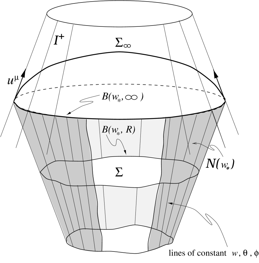
FIG. 1.: Geometry of the asymptotic slice $\Sigma_{\infty}$

In this figure one dimension of the two-surfaces $B(w_{*},R)$ is suppressed. The shaded, partially cut-away, conical surface depicts the null hypersurface ${\cal N}={\cal N}(w_{*})$ determined by a constant value $w=w_{*}$ of retarded time. Heuristically, in the limit $R\rightarrow\infty$ the $\Sigma$ slice spanning $B(w_{*},R)$ becomes the asymptotic slice $\Sigma_{\infty}$ which spans a round spherical cut of ${\cal I}^{+}$, and one should envision the spacelike slice $\Sigma_{\infty}$ as becoming null asymptotically. Although $\partial/\partial w$ is timelike everywhere in the physical spacetime ${\cal M}$ (at least in relevant exterior regions), the extension to ${\cal I}^{+}$ of $\partial/\partial w$ (in a conformal completion $\hat{\cal M}$ of ${\cal M}$) is a null vector which lies in ${\cal I}^{+}$. Again heuristically, on $B(w_{*},\infty)$ the $\Sigma_{\infty}$ hypersurface normal $u^{\mu}\partial/\partial x^{\mu}$ is $\partial/\partial w$.

REFERENCES

- [1] J. D. Brown and J. W. York, Phys. Rev. D47, 1407 (1993).
- [2] A reformulation in terms of Ashtekar variables of some of the results presented in [1] can be found in S. R. Lau, Class. Quantum Grav. 13, 1509 (1996).
- [3] See J. W. York, Phys. Rev. D33, 2092 (1986); B. F. Whiting and J. W. York, Phys. Rev. Lett. 61, 1336 (1988); J. D. Brown, E. A. Martinez, and J. W. York, Phys. Rev. Lett. 66, 2281 (1991); J. D. Brown and J. W. York, Jr., Phys. Rev. D47, 1420 (1993); to be published in The Black Hole 25 Years After, edited by C. Teitelboim and J. Zanelli (Plenum Press) (gr-qc/9405024); and references therein.
- [4] R. D. Hecht and J. M. Nester, Phys. Lett. A 217, 81 (1996).
- [5] See, for example, J. N. Goldberg in General Relativity and Gravitation, vol. 1, edited by A. Held (Plenum Press, New York and London, 1980).
- [6] See, for example, M. Walker, in Gravitational Radiation; NATO Advanced Study Institute, edited by Nathalie Deruelle and Tsvi Piran, (North-Holland, Amsterdam, 1983). Proceedings of the Les Houches school, two-21 June, 1982.
- [7] R. K. Sachs, Proc. Roy. Soc. London, Ser. A 270 103 (1962); R. K. Sachs, Phy. Rev. 128 2851 (1962).
- [8] R. Penrose and W. Rindler, Spinors and Space-time, Vol. 1 & 2 (Cambridge University Press, Cambridge, 1984).
- [9] R. Geroch, in Asymptotic Structure of Space-Time, edited by F. P. Esposito and L. Witten (Plenum Press, New York, 1977).
- [10] R. Arnowitt, S. Deser, and C. W. Misner, in Gravitation: An Introduction to Current Research, edited by L. Witten (Wiley, New York, 1962).
- [11] J. D. Brown, J. Creighton, and R. B. Mann, Phys. Rev. D50, 6394 (1994).
- [12] P. T. Chruściel, M. A. H. MacCallum, and D. B. Singleton, Phil. Trans. R. Soc. Lond. A 350, 113 (1994).
- [13] T. Dray and M. Streubel, Class. Quantum Grav. 1, 15 (1984).
- [14] A. J. Dougan, Class. Quantum Grav. 9, 2461 (1992).
- [15] A. Ashtekar and M. Streubel, Proc. R. Soc. A 376, 585 (1981).
- [16] W. T. Shaw, Class. Quantum Grav. 1, L33 (1984).
- [17] A. R. Exton, E. T. Newman, and R. Penrose, J. Math. Phys. 10, no. 9, 1566 (1969).
- [18] O’Neill, Barrett, Elementary Differential Geometry (Academic Press, New York, 1966).
- [19] See, for example, M. Spivak, A Comprehensive Introduction to Differential Geometry, Vol 5 (Publish or Perish, Boston, 1979).