Spectral Geometry and Causality

Abstract.

For a physical interpretation of a theory of quantum gravity, it is necessary to recover classical spacetime, at least approximately. However, quantum gravity may eventually provide classical spacetimes by giving spectral data similar to those appearing in noncommutative geometry, rather than by giving directly a spacetime manifold. It is shown that a globally hyperbolic Lorentzian manifold can be given by spectral data. A new phenomenon in the context of spectral geometry is observed: causal relationships. The employment of the causal relationships of spectral data is shown to lead to a highly efficient description of Lorentzian manifolds, indicating the possible usefulness of this approach.
Connections to free quantum field theory are discussed for both motivation and physical interpretation. It is conjectured that the necessary spectral data can be generically obtained from an effective field theory having the fundamental structures of generalized quantum mechanics: a decoherence functional and a choice of histories.

Introduction

Two experimentally verified theories describe at present the physical world: quantum field theory and general relativity. Both have been extremely successful in their tested ranges of applicability.

Quantum field theory, particularly implemented in the so-called standard model, describes the types and behavior of elementary particles as measured in accelerator experiments and as experienced by everyday contact with matter.

General relativity is concerned with the classical spacetime in which quantum field theory takes place. This spacetime, a four-dimensional Lorentzian manifold with events being its points, can have a complicated structure both locally and globally and can be influenced by the presence of classically understood matter.

Both quantum field theory as applied in the standard model and general relativity indicate intrinsically that they cannot be valid under very extreme circumstances. But moreover they are not fully compatible even under rather usual conditions with the problem being that matter is described by a quantum theory whereas spacetime interacting with the quantum matter is described classically.

For all these reasons it is believed that it should be possible to find a more advanced theory in which also gravity is quantized and in which both the compatibility problem for general relativity and quantum field theory and their internal problems are resolved.

Such theories have already been proposed, most notably string theory [1]. While the internal consistency of such a theory turns out to be a difficult problem, another issue arises once the theory is formulated. How can one relate it to the physical world? The interpretational side of a physical theory has at certain points of history not been trivial but here the question stands with a new urgency. Practically all measurements that are performed in experimental physics use implicitly the notion of classical spacetime. The measurements of positions and times play a dominant role, and there is a clear practical understanding of them. But in a theory where gravity is quantized, there is no classical spacetime in its postulates. The obvious conclusion is that unless one is able to recover from such a theory classical spacetime, at least in an approximative sense, the theory may be a nice piece of mathematics but does not make contact with the physical world and is as a physical theory rather useless.

This work is concerned with providing a tool for recovering classical spacetime from an advanced theory and is thus aimed at the interpretation of a quantum theory of gravity. It is assumed here that such a theory can first be simplified to an effective low energy theory which will look like a usual quantum field theory but without having specified spacetime yet. In such a situation no Lorentzian manifold is present, but there are many structures that contain what one can call spectral information. It comes from the structure of the algebra of observables of the effective theory and eventually from structures like the decoherence functional of generalized quantum mechanics. The problem is thus to describe classical spacetime by spectral data.

There is a theory doing just that for Riemannian spaces: A. Connes’ noncommutative geometry [2, 3]. Noncommutative geometry describes classical spaces by commutative algebras of functions on them together with some additional structures on them. It is actually more powerful than is needed here: Noncommutative geometry is able to deal even with noncommutative algebras not corresponding to any classical space. In an indirect way this fact is actually useful even in the present situation where only a classical space is wished for: The understanding of the general noncommutative case is more direct in separating out which concepts are of fundamental importance and which are from a broader perspective just particularities. One structure recognized in this way as being important, the spectral triple, will be especially useful in the considerations presented.

So in a more specific view the problem is to discuss how noncommutative geometry can be used to describe spacetime in the particular commutative case. Unfortunately, the present mathematical framework is able to deal only with spaces of Riemannian type, having a nonnegative distance between any two points. There it is very efficient in using spectral data: Practically all the geometric information is contained in just a few relatively simple structures. The question is whether the same is possible in the Lorentzian case.

The answer to this question is the main topic and result of this work. Compared to Riemannian spectral geometry there is a new phenomenon recognized: causal relationships. Inspired by the thorough discussion of causality in quantum field theory [4, 5, 6, 16, 17], its place in the framework of noncommutative geometry is found. With this understanding it is possible to show that again, as in Riemannian geometry, the spectral data exhibit a remarkable efficiency in the description of Lorentzian spaces, at least if they are globally hyperbolic which will be assumed throughout.

This gives hope that the adopted approach may turn out to be actually useful in the way it is wished to be useful from the physical context. Several remarks and conjectures on applications in physical interpretations are put forward. Many technical questions are left open for further considerations but have now a clearer formulation and context and can thus be attacked gradually.

The work is organized in the following way:

Section 1 discusses a free Weyl spinor field and the fermionic quantization of its covariant phase space.

The local and causal structures of this field theory are emphasized in Section 2.

Section 3 reviews briefly the spectral triple of Connes’ spectral geometry.

A naïve spectral description of Lorentzian globally hyperbolic manifolds is given in Section 4.

In Section 5 the information contained in causal relationships is discussed and used to obtain a rather compact description of spacetime. The view obtained is the main result of this work.

This is summarized in the conclusion.

1. Fermionic quantization of free Weyl spinor fields

The field theory considered in this paper will be that of a fermionic Weyl spinor field. This choice is maybe not overly surprising in view of the role played by such fields in the standard model of particle physics. The primary motivation is, however, the importance of spinor fields in spectral geometry as will become clear in Section 3.

The covariant phase space $\mathcal{S}$ of a classical free Weyl spinor field $\psi$ is the linear space of solutions of the equation of motion following from the action $S$,

(1) $$S[\psi] =Re\int_{\Omega}{\bar{\psi}D\psi d\Omega},$$

i.e., the Dirac equation

(2) $$D\psi =0.$$

Here $D$ is the Dirac operator, $\bar{\psi}$ is the Dirac adjoint of $\psi$ [7] and $\Omega$ is an arbitrarily chosen region of spacetime.

If the spacetime manifold $M$ is assumed to be globally hyperbolic (i.e., is topologically $\Sigma\times\mathbb{R}$, sliced by spacelike Cauchy surfaces diffeomorphic to the 3-dimensional manifold $\Sigma$ [8]) then there is a Hermitean inner product $s$ on the space of solutions $\mathcal{S}$ of the Dirac equation expressed as an integral over a spacelike Cauchy surface $\Sigma$,

(3) $$\bar{\phi}\circ s\circ\psi=\int_{\Sigma}{\bar{\phi}{\gamma}_{\mu}\psi{d\Sigma}^{\mu}}$$

Here ${d\Sigma}^{\mu}$ is the future directed hypersurface element induced from the spacetime volume element $d\Omega$. In order for $s$ to be a Hermitean inner product on the space of solutions $\mathcal{S}$, it has to be independent of the choice of $\Sigma$. Indeed, given two spacelike Cauchy hypersurfaces ${\Sigma}_{1}$ and ${\Sigma}_{2}$, the difference in the corresponding Hermitean inner products can be by Stokes’ theorem expressed by a spacetime integral over the region $\Omega$ enclosed by ${\Sigma}_{1}$ and ${\Sigma}_{2}$, vanishing in consequence of the equation of motion 2:

(4) $$\int_{{\Sigma}_{1}}{\bar{\phi}{\gamma}_{\mu}\psi{d\Sigma}^{\mu}}-\int_{{\Sigma}_{1}}{\bar{\phi}{\gamma}_{\mu}\psi{d\Sigma}^{\mu}}=\int_{\Omega}{\left(\bar{\phi}D\psi-\overline{D\phi}\psi\right)d\Omega}$$

The real part $\mu$ of the Hermitean inner product $s$,

(5) $$\bar{\phi}\circ\mu\circ\psi=Re\int_{\Sigma}{\bar{\phi}{\gamma}_{\mu}\psi{d\Sigma}^{\mu}}$$

is a real bilinear symmetric inner product on the phase space $\mathcal{S}$. Its inverse is the fermionic causal Green’s function ${\tilde{G}}_{F}$.

It can be shown [9] that the fermionic causal Green’s function ${\tilde{G}}_{F}$ has the meaning of the Poisson bracket $\{\bullet,\bullet\}$ of classical mechanics [10]:

(6) $$\{\bullet,\bullet\}={\tilde{G}}_{F}={\mu}^{-1}$$

Once the classical description of a system (e.g. a field) is known, one can make an educated guess of what the correct quantum theory is, i.e., one can quantize the field theory. In principle there are two rather different ways to do that, namely quantization by path integrals [11] and canonical quantization (see, e.g.[9, 10, 12]). Here the latter is chosen, since it leads more directly to an algebraic setting used in noncommutative geometry.

In fermionic canonical quantization, chosen in agreement with the spin-statistics theorem[5], one starts with the classical phase space $\mathcal{S}$ equipped with the symmetric inner product $\mu$. The functions on the classical phase space $\mathcal{S}$, the classical observables, are then replaced by elements in a noncommutative algebra, the algebra of observables following some rules which turned out to be useful in particular cases. The rules are as follows:

First, a special set $F(\mathcal{S})$ of function on the phase space has to be selected. The set $F(\mathcal{S})$ of chosen classical observables should be closed under taking the Poisson bracket $\{\bullet,\bullet\}$, i.e.,

(7) $$\{a,b\}\in F(\mathcal{S}) \text{ for $a,b\in F(\mathcal{S})$},$$

Second, a linear map $\hat{\psi}$ into a complex associative algebra $\mathbf{A}$ should be given,

(8) $$\hat{\psi}:F(\mathcal{S}) \rightarrow\mathbf{A}.$$

The map $\hat{\psi}$ should satisfy a commutation relation replacing the Poisson bracket by a commutator:

(9) $$\hat{\psi}(a)\hat{\psi}(b)+\hat{\psi}(b)\hat{\psi}(a)=i\hat{\psi}(\{a,b\})\text{ for all $a,b\in F(\mathcal{S})$},$$

and its image $\hat{\psi}(F(\mathcal{S}))$ should generate the algebra $\mathbf{A}$.

Note 1.

If $F(\mathcal{S})$ contains the constant functions on $\mathcal{S}$ (which have vanishing Poisson brackets with all other functions on $\mathcal{S}$), then their image under the mapping $\hat{\psi}$ must be in the centre of the algebra $\mathbf{A}$, and if $\mathbf{A}$ is central then the image of constant functions is proportional to the unit $\mathbf{1}$ in the algebra. A not very surprising addition to the quantization rules then usually is the requirement

(10) $$\hat{\psi}(k)=k\mathbf{1} \text{for all constant functions $k$ on $\mathcal{S}$}.$$

In general, one of the difficulties of these rules is the potentially complicated anticommutation relation (9), and another is the choice of $F(\mathcal{S})$. Obvious choices, like the space of all continuous functions on $\mathcal{S}$, are plagued by inconsistencies or by giving an algebra that is far too big compared with the one that gives a quantum theory in agreement experiment. To deal with this situation, additional information is usually necessary (see e.g. [12]), and even then it is a difficult problem. The situation radically simplifies for a free system (i.e. one with a linear phase space $\mathcal{S}$) as the one considered here. The correct choice of $F(\mathcal{S})$ is then the space of linear observables.

One can define the field operator $\Psi(f)$ for a classical solution $f\in\mathcal{S}$

(11) $$\Psi(f)=\hat{\psi}(\mu\circ f),$$

and write the anticommutation relation (9) in the form

(12) $$\Psi(f)\Psi(g)-\Psi(g)\Psi(f)=i(f\circ\mu\circ g)\mathbf{1} f,g\in\mathcal{S}$$ for .

The ${C}^{\ast}$-algebra of observables of the quantum field generated from this anticommutation relation is unique and independent of a completion of $\mathcal{S}$ [13, 14]. It has a unique minimal enveloping von Neumann algebra [13] having, up to unitary isomorphism, a unique regular irreducible representation by bounded operators in a Hilbert space. There is no information whatsoever in this algebra about the smooth structure of spacetime.

2. Local algebras of observables

If the ${C}^{\ast}$-algebra of observables is considered by itself, without reference to its origin, then it is sufficient to express the evolution of the field by automorphisms and the space of states by normed positive linear functionals (see [15]), but then the physical interpretation is completely lost.

A somewhat similar loss of interpretation can be observed if a classical system is judged on the basis of its phase space only, where canonical transformations can rather arbitrarily change the meaning of coordinates and momenta. It is possible to argue that, e.g., the topology of the phase space is specific to the system, but this is by no means sufficient to give a complete description if there actually is a fundamental distinction between coordinates and momenta.

As mentioned in Section 1, the algebra of observables does in this case not contain any information about spacetime.

Some structure has thus to be given to the algebra of observables of a quantum field in order to enable one to give its physical interpretation. One could, of course, just remember the whole construction of the algebra of observables, starting with the classical field. In a path integral approach this would not be so bad, since classical histories are part of that framework, but in an algebraic approach to quantum field theory, where the classical field has just the position of an effective approximation, this is definitely not what one would wish to do. The widely accepted solution is to give the algebra of observables the structure of a local algebra [6, 15]. The idea is to associate with each region of spacetime $\Omega$ a subalgebra $\mathbf{A}(\Omega)$ of the algebra $\mathbf{A}$ of observables. Thus one obtains a set of subalgebras indexed (not necessarily unambiguously) by the set $I$ of open subsets of spacetime.

For many technical purposes it is not necessary to keep the reference to spacetime, and only some properties of the index set $I$ are extracted and required. This is the case of the definition of a quasi-local algebra [6, 15]. However, since here interpretation is the main concern, the full link to spacetime will be required [16, 17].

Definition 1.

A ${C}^{\ast}$-algebra $\mathbf{A}$ together with a spacetime manifold $M$ is local if the following three conditions all hold:

1. For each open subset $\Omega$ of $M$ there is a central ${C}^{\ast}$-algebra $\mathbf{A}(\Omega)$, with $\mathbf{A}(\emptyset)=\mathbb{C}$, and $\mathbf{A}(M)=\mathbf{A}$.

2. For any collection $\{{\Omega}_{i}\}$ of open subsets of $M$ one has

   $$\mathbf{A}\left(\cup_{i}{\Omega}_{i}\right)=\overline{\langle\cup_{i}\mathbf{A}\left({\Omega}_{i}\right)\rangle}$$

   (On the right hand side of this equation is the closure of the algebraic envelope $\langle\cup_{i}\mathbf{A}\left({\Omega}_{i}\right)\rangle$ of $\cup_{i}\mathbf{A}\left({\Omega}_{i}\right)$.)

3. If the regions ${\Omega}_{1}$, ${\Omega}_{2}$ are not in causal contact, then the corresponding algebras $\mathbf{A}\left({\Omega}_{1}\right)$, $\mathbf{A}\left({\Omega}_{2}\right)$ commute in the Bose case and graded-commute in the Fermi case.

Example 1.

The quantized Weyl spinor field can be given the structure of a local algebra. The Green’s function ${\tilde{G}}_{F}$ of the field can be used to produce from any smooth density $\nu$ on the spacetime manifold $M$ a solution $f$:

(13) $${f}^{p}={({\tilde{G}}_{F})}^{pq}{\nu}_{q}$$

and to each solution $f$ one can by (11) associate a quantum observable $\Psi(f)$. Given a subset $\Omega$ of spacetime, the algebra $\mathbf{A}(\Omega)$ can be then generated by densities with support in $\Omega$. If the supports of two measures ${\nu}_{1}$, ${\nu}_{2}$ are not causally connected, then the corresponding classical solutions ${f}_{1}$, ${f}_{2}$ can be checked to have a vanishing product ${f}_{1}\circ\mu\circ{f}_{2}$, and the corresponding quantum observables $\Psi({f}_{1})$, $\Psi({f}_{2})$ thus anticommute.

A pleasant feature of the local algebra structure is that the ${C}^{\ast}$-subalgebras $\mathbf{A}(\Omega)$ (with $\Omega\in M$) of $\mathbf{A}$ are actually sufficient to reconstruct the spacetime $M$ as a topological space and to determine its causal structure, as observed by U.Yurtsever [16, 17].

3. Connes’ spectral triple

A geometric space may be described by its set of points with some additional structures, or, alternatively, by the algebra of functions on it, again with some additional structures. The first point of view is the one of classical geometry. The second may be taken as a starting point for a far more general and powerful theory, A. Connes’ noncommutative geometry [2], and is adopted here. In particular, a space can be encoded in the form of a spectral triple [3].

Definition 2.

A spectral triple $(\mathbf{A},\mathcal{H},D)$ is given by an involutive algebra of operators $\mathbf{A}$ in a Hilbert space $\mathcal{H}$ and a selfadjoint operator $D={D}_{\ast}$ in $\mathcal{H}$ such that

1. The resolvent ${(D-\lambda)}^{-1},\>\lambda\not\in\mathbb{R}$, of $D$ is compact

2. The commutators $[D,a]=Da-aD$ are bounded, for any $a\in\mathbf{A}$

The triple is said to be even if there is a hermitean grading operator $\gamma$ on the Hilbert space $\mathcal{H}$ (i.e. ${\gamma}^{\ast}=\gamma,\>{\gamma}^{2}=\mathbf{1})$ such that

(14) $$\gamma a =a\gamma a\in\mathbf{A}$$ for all

(15) $$\gamma D =-D\gamma$$

Otherwise the triple is called odd

Note 2.

This section is only concerned with introducing the spectral triple and mentioning its properties to be used in the applications. From that it is not fully clear why one should be interested in exactly this kind of structure, so some motivation is clearly missing here. See however [2, 3] for the deep and solid structure of noncommutative geometry that is supporting the spectral triple.

The following example is of great importance.

Example 2.

On a compact Riemannian spin manifold $M$ there is canonically the following spectral triple $({C}^{\infty}(M),{L}^{2}(M,S),D)$, the Dirac triple [2], [3]. Here ${C}^{\infty}(M)$ is the commutative algebra of smooth complex functions on $M$, ${L}^{2}(M,S)$ is the Hilbert space of square integrable sections of the complex spinor bundle $S$ over $M$ and D is the Dirac operator. The algebra of functions ${C}^{\infty}(M)$ acts on the Hilbert space ${L}^{2}(M,S)$ by pointwise multiplication

(16) $$(f\psi)(p) =f(p)\psi(p) f\in{C}^{\infty}(M),\psi\in{L}^{2}(M,S),p\in M$$ for all

and the commutator with the Dirac operator $$D f$$ with a function is

(17) $$[D,f] =\gamma df f\in{C}^{\infty}(M)$$ for .

$\gamma$ is the Clifford map from the cotangent bundle into operators on ${L}^{2}(M,S)$.

In Example 2 the algebra was taken to be ${C}^{\infty}(M)$. Such a choice contains a lot of information and is actually not necessary. In the definition of the Dirac spectral triple it is sufficient to take instead of ${C}^{\infty}(M)$ any algebra $\mathbf{A}$ that has the same weak closure (double commutant) ${\mathbf{A}}^{{}^{\prime\prime}}$ as has ${C}^{\infty}(M)$. Such an algebra does not necessarily contain any information about the topology or differential structure of $M$ whatsoever. From $\mathbf{A}$ alone only $M$ as a set of points can be obtained as the spectrum of $\mathbf{A}$. The rest, however, can then be recovered from the structure of the spectral triple including the notion of smooth functions and Lipschitz functions. Lipschitz functions with Lipschitz constant $1$ can then be used to define a distance function $d$ on $M$. This means that a Riemannian spin manifold can be replaced by a spectral triple without the loss of any information about it. The facts are summarized in Proposition 1 (see [3]).

Proposition 1.

Let $(\mathbf{A},{L}^{2}(M,S),D)$ be the Dirac spectral triple associated to a compact Riemannian spin manifold M. Then the compact space $M$ is the spectrum of the commutative ${C}^{\ast}$-algebra norm closure of

(18) $${\mathbf{A}}_{B} =\{a\in{\mathbf{A}}^{{}^{\prime\prime}}\mid[D,a]\text{ bounded}\}$$

while the geodesic distance $$d M$$ on is given by

(19) $$d(p,q) =\sup{\{\mid f(p)-f(q)\mid;f\in{\mathbf{A}}_{B},\parallel[D,f]\parallel\leq 1\}}$$

It is now in question whether one can reconstruct from a spectral triple a manifold if one is not assured that the spectral triple actually comes from a manifold. With some additional conditions it will certainly be possible to prove in the future a theorem in this direction. One helpful tool for this purpose is a real structure $J$ on the spectral triple [3], [18].

Example 3.

In the case of the Dirac spectral triple of Example 2 a real structure is given by the charge conjugation composed with complex conjugation (see [7]).

Before giving its general definition it should be mentioned that for simply connected spaces the real structure ensures that the spectrum of a spectral triple will have the homotopy type of a closed manifold [3], [18]. In addition to that, its dimension is governed by the spectrum of the Dirac operator [19]. So a theorem examining which commutative spectral triples are classical Riemannian manifolds is not out of sight. The considerations of the next sections would be best motivated by such a theorem but making use of it is at this point probably premature.

Definition 3.

A real structure $J$ on the spectral triple $(\mathbf{A},\mathcal{H})$ is an antilinear isometry $J$

(20) $$J:\mathcal{H} \rightarrow\mathcal{H}$$

such that

(21) $$Ja{J}^{-1} ={a}^{\ast} a\in\mathbf{A}$$ for all

(22) $${J}^{2} =\epsilon$$

(23) $$JD ={\epsilon}^{{}^{\prime}}DJ$$

(24) $$J\Gamma ={\epsilon}^{{}^{\prime\prime}}\Gamma J$$

where the signs $\epsilon,{\epsilon}^{{}^{\prime}},{\epsilon}^{{}^{\prime\prime}}\in\{-1,+1\}$ are given by the following table with $\nu$ being the dimension of the space $mod\>8$:

(25) $$\begin{array}[]{|c|c|c|c|c|c|c|c|c|}\hline\cr\nu&0&1&2&3&4&5&6&7\\ \hline\cr\epsilon&1&1&-1&-1&-1&-1&1&1\\ \hline\cr{\epsilon}^{{}^{\prime}}&1&-1&1&1&1&-1&1&1\\ \hline\cr{\epsilon}^{{}^{\prime\prime}}&1&&-1&&1&&-1&\\ \hline\cr\end{array}$$

Note 3.

The sign ${\epsilon}^{{}^{\prime\prime}}$ in Table (25) is shown for even dimensions only, since for Riemannian spin manifolds only in that case the grading (helicity) operator ${\Gamma}$ preserves the irreducible spin representation and has thus a good meaning in it. In the odd case it is assumed that only one of the two irreducible representations is chosen and since $\Gamma$ switches between the two irreducible representations it has no meaning just in one of them. More details on spinors can be found in [7]. Also the periodicity $mod\>8$ of Table (25), a manifestations of the spinorial chessboard is explained there.

4. Spacetime in spectral geometry

Here a Lorentzian globally hyperbolic spacetime manifold will be characterized by spectral data. This cannot be done directly by Connes’ spectral triple (see Definition 2) since it is well suited for the description of generalized Riemannian spaces only. This is obvious, e.g., from the distance function (19), which cannot be negative. A simple idea to avoid this difficulty is to foliate the spacetime $M$ by a family of spacelike Cauchy slices ${\Sigma}_{t}$ with $t\in\mathbb{R}$ a coordinate time (see Figure 1). Each hypersurface ${\Sigma}_{t}$ is then Riemannian and can be characterized by a family of Dirac spectral triples $\left({L}^{\infty}({\Sigma}_{t}),{L}^{2}({\Sigma}_{t},S),{D}_{t}\right)$ (see Example 2 and Proposition 1) together with some additional information on how the spacelike slices ${\Sigma}_{t}$ are related to each other. In particular, the normal distance between two infinitesimally close Cauchy surfaces ${\Sigma}_{t}$ is encoded by the lapse function $N$ (see [21] and Figure 1). The only further information needed is the identification ${i}_{t}:{\Sigma}_{t}\rightarrow{\Sigma}_{0}$ of points which lie on the same curve normal to the hypersurfaces. This can be established in the spectral data by specifying an automorphism ${i}_{t}^{\ast}:{L}^{\infty}({\Sigma}_{0})\rightarrow{L}^{\infty}({\Sigma}_{t})$

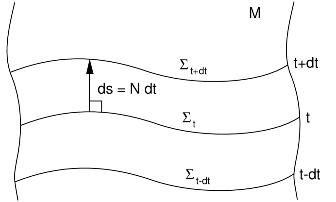
Figure 1. A Cauchy foliation. The globally hyperbolic manifold $M$ can be sliced by spacelike Cauchy surfaces ${\Sigma}_{t}$. Each of them can be characterized by a Dirac spectral triple $\left({L}^{\infty}({\Sigma}_{t}),{L}^{2}({\Sigma}_{t},S),{D}_{t}\right)$ with ${L}^{\infty}({\Sigma}_{t})$ being the algebra of essentially bounded functions on ${\Sigma}_{t}$, ${L}^{2}({\Sigma}_{t},S)$ being the spinor bundle over ${\Sigma}_{t}$ and ${D}_{t}$ being the Dirac operator on ${\Sigma}_{t}$. The normal distance between infinitesimally close Cauchy surfaces ${\Sigma}_{t}$, ${\Sigma}_{t+dt}$ is characterized by the lapse function $N$ on ${\Sigma}_{t}$. $N$ can be thought of as an element in the algebra ${L}^{\infty}({\Sigma}_{t})={\left({C}^{\infty}({\Sigma}_{t})\right)}^{{}^{\prime\prime}}$, the double commutant of the algebra of smooth functions.

Since the square integrable sections of the spin bundles over the Cauchy surfaces ${\Sigma}_{t}$, $t\in\mathbb{R}$ are valid Cauchy data for weak solutions of the equation of motion of a Weyl spinor field on M, there is a preferred isomorphism between the spin bundles ${L}^{2}({\Sigma}_{t},S)$ and the space of solutions $\mathcal{S}$ of Weyl spinors. This means that all spectral triples can be understood to share the same Hilbert space $\mathcal{S}$.

Summarizing, a globally hyperbolic spacetime can be described using spectral data by

• a family of spectral triples $({\mathbf{C}}_{t},\mathcal{S},{D}_{t})$ with ${\mathbf{C}}_{t}$ a commutative algebra of bounded operators on $\mathcal{S}$ and ${D}_{t}$ Hermitean (possibly unbounded) on $\mathcal{S}$

• a family of lapse functions ${N}_{t}\in{\mathbf{C}}_{t}$

• an automorphism ${i}^{\ast}$ between any two of the commutative algebras ${\mathbf{C}}_{t}$

Note 4.

Usually it is not required that the identification of Cauchy surfaces has to be done along normal lines. Then the deviation of of the direction of identification from the normal one has to be characterized by a shift vector field $\vec{N}$ on the Cauchy surfaces [21]. The restriction to the case $\vec{N}=0$ here avoids the necessity of a replacement of vector fields by spectral concepts.

The above description agrees with [20] except that there the automorphism ${i}^{\ast}$ is omitted. That omission seems to make the spectral data appear incomplete from the point of view presented there.

It is now possible to describe the quantum field theory for Weyl spinors on the spacetime specified by the spectral data. Since the Hilbert space $\mathcal{S}$ in the spectral data is taken to be the space of classical solutions equipped with the canonical Hermitean inner product (3), this is entirely trivial: The quantum field algebra of observables is just the Clifford algebra generated from $\mathcal{S}$ by the anticommutation relation (12).

This completes the discussion of quantum field theory on spacetime using a spectral approach but not taking in account the causal structure information present in the problem. This is a natural place to reflect on the above with a few comments.

From the point of view of the motivations, one would wish to start from an algebra of quantum observables, to specify the spectral data, and then to construct, if possible, classical spacetime. Such an approach will however bring rather difficult problems: At least in the cases where one hopes to obtain a spacetime that is a topological or smooth manifold, one would wish to have the one-parameter family ${\mathbf{C}}_{t}$ in some sense continuous or smooth. (It may be viewed as a continuous or smooth algebra bundle over $\mathbb{R}$). This is an important, but on the other hand technical, issue. Instead of discussing it satisfactorily, the treatment will rely on the case studied here starting with a classical spacetime, producing the space of solutions $\mathcal{S}$ of the Weyl spinor field on it and obtaining by quantization the field algebra $\mathbf{A}$. Then all the facts can be viewed backwards, starting with the field algebra $\mathbf{A}$. This is clearly dishonest to the motivations in using as its input what should be abandoned in the first place: classical spacetime. On the other hand this allows one to go through all the way from the quantum algebra to spacetime avoiding some, in general difficult, arguments bridged by the particular features of this not-so-elegant example. The result is then an understanding of what is important, and with this, one can then gradually face the technically difficult points. This approach has worked so far extremely well in noncommutative geometry. In this context, the aim here is to gain an understanding only, thus considering the example as a valid approach.

For a view starting from the quantum field algebra according to the above motivations, it would also be desirable to have a deeper justification of the introduced structures, particularly for the family of operator algebras ${\mathbf{C}}_{t}$ and the family of operators ${D}_{t}$ on the space $\mathcal{S}$ generating the algebra of observables $\mathbf{A}$. It will be suggested here in the form of two conjectures that this may eventually be possible.

Conjecture 1.

Another way to look at the family of commutative algebras ${\mathbf{C}}_{t}$ will be offered now. For a given value of the parameter $t={t}_{0}$, the algebra ${\mathbf{C}}_{{t}_{0}}$ splits the space $\mathcal{S}$ into orthogonal subspaces by spectral projections. On the quantum level this means that the field algebra $\mathbf{A}$ is given preferred mutually commuting subspaces. In the case in which the Hilbert space is finite dimensional, these spaces are complex one dimensional. It is conjectured that this structure is sufficient to determine a preferred complete set of commuting projectors in the algebra of observables $\mathbf{A}$ or eventually in its (unique) minimal enveloping von Neumann algebra. If that is the case, then the choice of ${\mathbf{C}}_{{t}_{0}}$ may be understood as the choice of a set of histories in generalized quantum mechanics [22, 23, 24, 25]. This would to a large degree justify the introduced structures from a very fundamental point of view.

Conjecture 2.

If Conjecture 1 is in some way correct, then the family ${D}_{t}$ of Hermitean operators on $\mathcal{S}$ can be recovered from the decoherence functional of generalized quantum mechanics on histories of the quantum field $\mathbf{A}$.

These conjectures are a topic of future research. They are stated here only to show that what was reached so far is really following the call of the motivations put forward in the Introduction, which would not be so easy to see otherwise.

5. Spectral data and the causal structure of spacetime.

The spectral data describing spacetime as presented in the previous section are sufficient. But they do not take into account the fact that causal structure information is also stored in the family of spectral triples in a way that was not yet exploited.

To understand that, consider two spacelike Cauchy surfaces ${\Sigma}_{0}$, ${\Sigma}_{1}$ on the spacetime manifold (see Figure 2). They are described by the spectral triples $({\mathbf{C}}_{0},\mathcal{S},{D}_{0})$, $({\mathbf{C}}_{1},\mathcal{S},{D}_{1})$. Given two points ${p}_{0}$, ${p}_{1}$ on these Cauchy surfaces (${p}_{0}\in{\Sigma}_{0}$, ${p}_{1}\in{\Sigma}_{1}$) it is now possible just to decide whether they are in causal contact or not. If and only if the points ${p}_{0}$, ${p}_{1}$ are not in causal contact, the value of the Weyl spinor field at the point ${p}_{0}$ cannot influence the value of the field at the point ${p}_{1}$. In more precise terms on can say that there exist open neighborhoods $\mathcal{U}({p}_{0})$, $\mathcal{U}({p}_{1})$ of the points ${p}_{0}$, ${p}_{1}$ in ${\Sigma}_{0}$, ${\Sigma}_{1}$ such that any solution $\psi$ of the equation of motion of the Weyl spinor field with Cauchy data on ${\Sigma}_{0}$ supported in $\mathcal{U}({p}_{0})$ has a vanishing inner product with any solution $\phi$ with Cauchy data on ${\Sigma}_{1}$ supported in $\mathcal{U}({p}_{1})$. To identify solutions in $\mathcal{S}$ which have Cauchy data on ${\Sigma}_{i}$ supported in a certain region $\mathcal{U}({p}_{i})\subset{\Sigma}_{i}$ from the spectral data is easy: they are just given as elements of the ranges of the spectral projection corresponding to $\mathcal{U}({p}_{i})$.

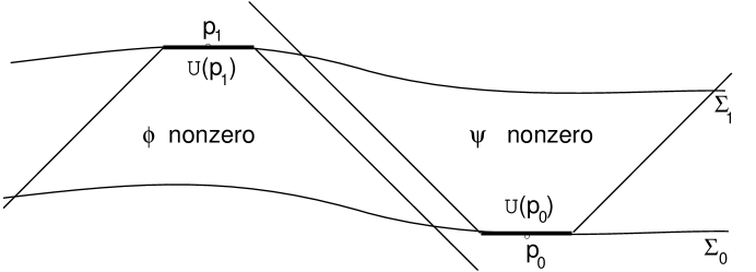
Figure 2. Causal contact. Any solution $\psi$ with Cauchy data on ${\Sigma}_{0}$ supported in $\mathcal{U}({p}_{0})$ has a vanishing inner product with any solution $\phi$ with Cauchy data on ${\Sigma}_{1}$ supported in $\mathcal{U}({p}_{1})$. The points ${p}_{0}$, ${p}_{1}$ are not causally connected.

Note 5.

If one is willing to use generalized eigenvectors then causal contact can be expressed in the following way. A (generalized) solution with Cauchy data on ${\Sigma}_{0}$ supported in the point ${p}_{0}$ is a generalized eigenvector of the algebra ${\mathbf{C}}_{0}$ satisfying

(26) $$a\psi=a({p}_{0})\psi a\in{\mathbf{C}}_{0}$$ for ,

with $a({p}_{0})$ being the value of the function $a$ at the point ${p}_{0}$. The vector $\psi$ can then be for briefness called an eigenvector of point ${p}_{0}$. Then two points are not in causal contact if and only if all their eigenvectors are orthogonal.

One can now summarize:

Observation 1.

Using the family ${\mathbf{C}}_{t}$ of commutative algebras represented on the Hilbert space $\mathcal{S}$ of solutions, one can recover spacetime as a set of points and find by the above procedure which points are in causal contact, using the Hermitean inner product on $\mathcal{S}$.

This observation is of central importance. Before using it to reduce the spectral data necessary to describe a Lorentzian spacetime, a two connections will be made.

First, from the point of view of differential equations it is not surprising that the Hermitean inner product on $\mathcal{S}$ contains information on the causal structure, since as mentioned in Section 1 the real part of it is the inverse of the causal Green’s function.

Second, from the point of view of quantum field theory the orthogonality of classical solutions with Cauchy data locally supported around two points ${p}_{0}$, ${p}_{1}$ has as its consequence (or, if one wishes, as its origin) the graded commutativity of the corresponding ${C}^{\ast}$-subalgebras of the local algebra $\mathbf{A}$ of observables generated from $\mathcal{S}$. This is the point where the notion of causality makes contact with Section 2 and with some of the motivations for this work given in the Introduction.

Now the consequences of Observation 1 will be discussed. First of all, the family of spectral triples $({\mathbf{C}}_{t},\mathcal{S},{D}_{t})$ of Section 3 contains already all necessary information about spacetime and no automorphism ${i}^{\ast}$ between the algebras ${\mathbf{C}}_{t}$ and no lapse function $N$ need to be specified. Indeed, by knowing the geometry of the Cauchy surfaces ${\Sigma}_{t}$ corresponding to the spectral triples $({\mathbf{C}}_{t},\mathcal{S},{D}_{t})$ and the causal structure one can find the normal identifications of points and the normal distances between infinitesimally close Cauchy surfaces (see Figure 3).

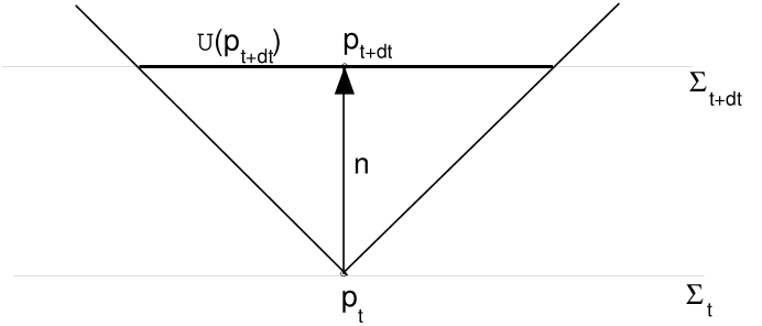
Figure 3. The geometry of Cauchy surfaces, causal contact and the geometry of spacetime. The point ${p}_{t}$ on ${\Sigma}_{t}$ has as its region of causal contact on ${\Sigma}_{t+dt}$ the disk $\mathcal{U}({p}_{t+dt})$ (including its bounding sphere). The square of the radius of the sphere is the negative of the square of the normal spacetime distance between the Cauchy surfaces ${\Sigma}_{t}$, ${\Sigma}_{t+dt}$, and the center ${p}_{t+dt}$ of the sphere $\mathcal{U}({p}_{t+dt})$ is the point reached by the normal vector $n$ based in ${p}_{t}$.

Thus a large part of the spectral data can be just left out, and the remaining family of spectral triples gives now a quite efficient description. But it is still considerably redundant. To see this is not difficult: If the metric information contained in the operators ${D}_{t}$ is omitted, then the conformal structure of spacetime is still rigidly fixed. But not all metrics are conformally related, and thus the ${D}_{t}$ determining the metric on the Cauchy surfaces cannot be chosen at will but have to agree with the conformal structure. This means that the spectral data of spacetime can be further reduced. How this has to be done in a useful way will be left for consideration in the future. But even without that a conceptual result is appearing: The spectral data describing a Lorentzian manifold do so in a very efficient way. This result based on Observation 1 is the main claim of this work.

Note 6.

There is a way of giving less redundant spectral data, if one is willing to lose metric information and keep just the conformal structure of spacetime. It is shown in [2] that for building just differential geometry without metric information, it is sufficient to take, instead of the spectral triple with an unbounded operator $D$, the same spectral triple but with $D$ replaced by $F=sgn\>D$, the sign of the operator $D$. This is actually a grading operator on $\mathcal{S}$ since ${F}^{2}=\mathbf{1}$. Thus the spectral triple $({\mathbf{C}}_{t},\mathcal{S},{F}_{t})$ with a family of grading operators contains the topological and causal as well as differential geometric information on spacetime.

Note 7.

One may wonder where the efficiency of the spectral data in the presented description comes from. In the case of the spectral triple A. Connes argued [2, 3] that most of the information is not in the algebra of the triple, giving basically just a set of points, nor in the chosen Hermitean operator, fully described by its spectrum, but in the relationship between them. This explanation can be used here again: Most of the information in the spectral data is not in the commutative algebras ${\mathbf{C}}_{t}$ represented on $\mathcal{S}$ but in the relationships between them. Indeed, the strong causal structure is purely a result of this.

Conclusion

Motivated by the need to recover classical spacetime from a theory of quantum gravity in order to achieve the theory’s physical interpretation, the thesis examines the possibility of describing classical Lorentzian spacetime manifolds by spectral data.

Following in Section 4 a naïve Hamiltonian approach, the spectral data for a Lorentzian manifold are specified as a family of A. Connes’ spectral triples with a common Hilbert space and additional structures known from Hamiltonian general relativity: a family of lapse functions and an identification of Cauchy surfaces implemented by isomorphisms of the algebras in the spectral triples. This gives a complete description of spacetime, trivially extended to a free quantum field theory on spacetime.

However, in Section 5 it is realized that the spectral description of spacetime automatically contains unused information on causal relationships. The use of this information leads to a significant reduction of the spectral data. The family of lapse functions and the identification of Cauchy surfaces can be completely left out, and still there is considerable redundancy in the data present. The discovery of the place of causal relationships in spectral geometry thus leads to a very efficient spectral description of spacetime. This is the main result of this thesis.

With the result attained here, there are now two well motivated problems of conceptual importance:

1. The remaining redundancy in the spectral data should be removed and the result put into a useful form to be recognized as standard.

2. The way in which the result may fit into an interpretation of quantum gravity should be clarified, possibly along the lines of Conjectures 1 and 2

Moreover, there are also many further points of technical nature, to be worked out. To suggest just one of them as an example, it would be desirable to have a usefully formulated expression for spacetime distances.

With the insight obtained here, these questions are now open to future investigations.

References

- [1] E. Witten, Phys. Today 49, 24 (1996).
- [2] A. Connes, Noncommutative geometry (Academic Press, San Diego, 1994).
- [3] A. Connes, Journal of Math. Physics 36, 11 (1995).
- [4] R. Haag and D. Kastler, J. Math. Phys. 5, 848 (1964).
- [5] R. F. Streater and A. S. Wightman, PCT, spin and statistics, and all that (W. A. Benjamin, Reading, Massachusetts, 1964).
- [6] R. Haag, Local quantum physics: fields, particles, algebras (Springer-Verlag, Berlin Heidelberg, 1992).
- [7] P. Budinich and A. Trautman, The spinorial chessboard (Springer-Verlag, Berlin Heidelberg, 1988).
- [8] R. M. Wald, Quantum field theory in curved spacetime and black hole thermodynamics (The University of Chicago Press, Chicago and London, 1994).
- [9] B. S. DeWitt, Dynamical theory of groups and fields (Gordon and Brench, New York, 1965).
- [10] B. S. DeWitt, The space-time approach to quantum field theory (North Holland, Amsterdam, 1984).
- [11] R. P. Feynman and A. R. Hibbs, Quantum mechanics and path integrals (McGraw-Hill, New York, 1965).
- [12] N. M. J. Woodhouse, Geometric quantization, 2nd ed. (Oxford University Press, New York, 1991).
- [13] R. Plymen and P. Robinson, Spinors in Hilbert space (Cambridge University Press, Cambridge, 1994).
- [14] O. Bratteli and D. W. Robinson, Operator algebras and quantum statistical mechanics (Springer-Verlag, New York, 1981), Vol. II.
- [15] O. Bratteli and D. W. Robinson, Operator algebras and quantum statistical mechanics (Springer-Verlag, New York, 1979), Vol. I.
- [16] U. Yurtsever, Class. Quant. Grav. 11, 999 (1994).
- [17] U. Yurtsever, Class. Quant. Grav. 11, 1013 (1994).
- [18] A. Connes, Gravity coupled with matter and the foundation of non-commutative geometry, e-print: hep-th/9603053.
- [19] P. B. Gilkey, Invariance theory, the heat equation, and the Atiyah-Singer index theorem (Publish or Perish, Wilmington, Delaware, 1984).
- [20] E. Hawkins, Hamiltonian gravity and noncommutative geometry, e-print: qc-qc/9605068.
- [21] C. W. Misner, K. S. Thorne, and J. A. Wheeler, Gravitation (Freeman, San Francisco, 1973).
- [22] J. B. Hartle, Space-time quantum mechanics and the quantum mechanics of spacetime, Gravitation and quantizations, Les Houches Summer Proceedings, Vol.LVII (North Holland, Amsterdam, 1992).
- [23] C. J. Isham, J. Math. Phys 35, 2157 (1994).
- [24] C. J. Isham and N. Linden, J. Math. Phys 35, 5452 (1994).
- [25] C. J. Isham, N. Linden, and S. Schreckenberg, J. Math. Phys 35, 6360 (1994).