Cosmological solutions of the Brans-Dicke theory are investigated by including a quantum effect coming from 1-loop correction of matter fields that couple to the scalar field. As the most serious result we face a cosmological “constant” in the original conformal frame which is shown to be “physical” after a careful analysis of the time variable employed in any of the conventional approaches. We find an “attractor” solution featuring no expansion during the radiation-dominated eras. To evade this unacceptable consequence, we suggest to modify one of the fundamental premises of the model, rendering the scalar field almost “invisible.”

1 Introduction

Among many versions of the scalar-tensor theory of gravitation, the prototype Brans-Dicke (BD) model [1] is unique for the following four assumptions on the scalar field: (i) a nonminimal coupling of the simplest form; (ii) masslessness; (iii) no self-interaction; (iv) no direct matter coupling.

Although the model may not be fully realistic, it still seems to deserve further scrutiny as a testing ground of many aspects of wider class of the scalar-tensor theories. The model has been studied, however, mainly as a classical theory. We attempt to take quantum effects due to the matter coupling into account. It has been argued that composition-independence that entails from the assumption (iv) above would be violated as a quantum correction [2]. We came to realize, however, that the suspected contribution is canceled by other terms arising from regularization; WEP is in fact a well-protected and robust property of the model beyond the classical level.

We discuss in this note another quantum effect which, as it turns out, has serious cosmological consequences, beyond the extent of remedy expected by adjusting the fundamental parameter of the model. For a possible way out we suggest to modify the assumption (iv), making the scalar field almost “invisible,” thus reconciling with the absence of experimental evidences, still playing a cosmological role. We also discuss how the scalar field acquires a nonzero self-mass due to the matter coupling, even having started with the classical assumption (ii), but likely in an entirely insignificant manner in practice.

We start with the basic Lagrangian

$${\cal L}=\sqrt{-g}\left(\frac{1}{2}F(\phi)R-\epsilon\frac{1}{2}g^{\mu\nu}\partial_{\mu}\phi\partial_{\nu}\phi+L_{\rm m}\right),$$ (1)

with

$$F(\phi)=\xi\phi^{2}.$$ (2)

We use the unit system of $8\pi G=1.$ The scalar field $\phi$ and the constant $\xi$ are related to the original notation $\varphi$ and $\omega$, respectively, by

$$\varphi=\frac{1}{2}\xi\phi^{2},\quad{\rm and}\quad\omega=\frac{1}{4\xi}.$$ (3)

We also allow $\epsilon=\pm 1$, a minimum extension of the original model to avoid an immediate failure. As we see shortly, $\epsilon=-1$ does not necessarily imply a ghost in the final result.

As the matter Lagrangian we choose, according to the assumption (iv),

$$L_{\rm m}=-\overline{\psi}\left(D/+m_{0}\right)\psi,$$ (4)

where $\psi$ stands for a simplified representative of the (spinor) matter field.

In spite of (iv) $\phi$ couples in effect to the matter field in the field equation. This is inconvenient, however, when we try to apply the conventional technique of quantum field theory to the $\phi\,$-matter coupling. For this reason we apply a conformal transformation such that the nonminimal coupling is eliminated [3]:

$$g_{\mu\nu}=\Omega^{-2}g_{*\mu\nu},\quad{\rm with}\quad\Omega=\left(\xi\phi^{2}\right)^{1/2}.$$ (5)

Notice that we should have

$$\xi>0,$$ (6)

in order to ensure that the sign of the line element remains unchanged.

We in fact find that (1) is now put into the form

$${\cal L}=\sqrt{-g_{*}}\left(\frac{1}{2}R_{*}-\frac{1}{2}g^{\mu\nu}_{*}\partial_{\mu}\sigma\partial_{\nu}\sigma+L_{*m}\right),$$ (7)

expressed in terms of the new metric $g_{*\mu\nu}$ and the field $\psi_{*}=\Omega^{-3/2}\psi$. Also the canonical scalar field is now $\sigma$ as defined by

$$\phi(\sigma)=\phi_{0}\;e^{\beta\sigma},$$ (8)

where

$$\beta=\frac{1}{\sqrt{6+\epsilon\xi^{-1}}}=\sqrt{\frac{4\pi G}{3+2\epsilon\omega}}.$$ (9)

We emphasize that $\sigma$ is not a ghost if

$$\beta^{2}>0,$$ (10)

even if $\epsilon=-1$ [4]; “mixing” between the scalar field and (spinless part of) the metric field provides sufficient amount of positive contribution to overcome the negative kinetic part. The condition (10) is equivalent to

$$\epsilon\xi^{-1}>-6,\quad{\rm or}\quad\epsilon\omega>-\frac{3}{2}.$$ (11)

We now have a direct $\sigma$-matter coupling expressed in terms of the interaction Hamiltonian to which usual perturbation method is readily applied. We point out, however, that EEP, hence WEP as well, remains intact because the deviation from geodesic arising from the transformation (5) is given entirely in terms of $\sigma$ which is independent of any specific properties of individual particles; the fact that any motion is independent of the mass, for example, verified in one conformal frame obviously survives conformal transformations.

We call the conformal frames before and after the conformal transformation J frame and E frame, respectively.

2 Quantum effect

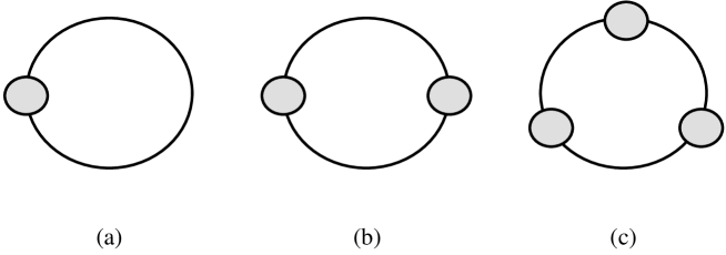
In E frame, in which we hereafter suppress the symbol $*$ for simplicity, we consider one-loop diagrams as shown in Fig. 1, due to the interaction

$$H^{\prime}_{1}=m_{0}\xi^{-1/2}\phi^{-1}(\sigma)\overline{\psi}\psi,$$ (12)

coming originally from the mass term in J frame.

As will be shown, $\sigma$ may keep moving with time, and so does the mass. But $\sigma$ moves so slowly compared with any of the microscopic time-scales, that the mass $m(t)$ at each epoch will be defined by

$$m(t)=m_{0}\xi^{-1/2}\phi^{-1}(\sigma(t)).$$ (13)

Now consider the 1 -$\phi^{-1}$ diagram (a). Its contribution is given by the potential of $\sigma$;

$$V_{1}(\sigma)=im(\sigma)\int d^{4}p\,{\rm Tr}\!\left(\frac{1}{m(\sigma)+ip/}\right).$$ (14)

Our consideration will be restricted to the Universe which is sufficiently late to justify to ignore the effect of temperature and spacetime curvature.

The integral in (14) is quadratically divergent, but is expected to vanish if there is supersymmetry because the fermionic contribution given by (14) is canceled by the same contribution from the bosonic partner. The cancellation would not be complete, however, if supersymmetry is broken at the mass scale

$$M_{\rm ssb}=rm,$$ (15)

where the ratio $r$ of $M_{\rm ssb}$ to $m$, a representative of ordinary particles taken roughly of the order of GeV, would be $\sim 10^{3}$–$10^{4}$, which we naturally choose to be a true constant.

The result may be given by

$$V_{1}(\sigma)=C_{1}r^{2}m^{4}=V_{1}(0)e^{-4\beta\sigma},$$ (16)

where

$$V_{1}(0)=C_{1}r^{2}\left(m_{0}\xi^{-1/2}\phi_{0}^{-1}\right)^{4},$$ (17)

with $C_{1}$ most likely of the order 1. Its sign, however, may not be known precisely because it depends on the details of supersymmetry breaking. If $C_{1}>0$, (16) gives a positive exponential potential that would drive $\sigma$ toward infinity. We assume this to be the case.

3 Cosmology

We now consider the cosmological equations with a classical potential $V=V_{1}$ which is the only potential due to the assumption (iii):

$$3H^{2}=\frac{1}{2}\dot{\sigma}^{2}+V+\rho,\vspace{.5em}$$ (18)

$$\ddot{\sigma}+3H\dot{\sigma}+V^{\prime}(\sigma)=0,\vspace{.3em}$$ (19)

$$\dot{\rho}+4H\rho=0,$$ (20)

where $\rho$ is the matter density which we assume, for the moment, to be relativistic. We also ignored possible terms representing the coupling between $\sigma$ and $\rho$. This would be justified for our purposes as long as we consider late epochs during which the coupling is sufficiently weak [4].

With $V=V_{1}$, a set of analytic solutions of (18)–(20) are obtained:

$$a(t) = t^{1/2},$$ (21)

$$\sigma(t) = \frac{1}{2\beta}\ln t,$$ (22)

$$\rho(t) = \frac{3}{4}\left(1-\frac{1}{4}\beta^{-2}\right)t^{-2},$$ (23)

with

$$V_{1}(0)=\frac{1}{16\beta^{2}}.$$ (24)

Notice that the condition $\rho>0$ is met if

$$\beta^{-2}<4,\quad{\rm or}\quad\epsilon\xi^{-1}<-2,$$ (25)

which, combined with (6), is satisfied only if $\epsilon=-1$. This is the reason why we decided to allow an “apparent” ghost in J frame. Then (25) translates into

$$\xi^{-1}>2,\quad{\rm or}\quad\omega>\frac{1}{2},$$ (26)

a much milder constraint than those derived from the observation. With $\epsilon=-1$, however, (11) implies

$$\xi^{-1}<6,\quad{\rm or}\quad\omega<\frac{3}{2},$$ (27)

which is ruled out immediately by the solar-system experiments, giving $\omega\mbox{\raisebox{-3.00003pt}{$\stackrel{{\scriptstyle>}}{{\sim}}$}}10^{3}$ [7]. We nevertheless continue our analysis as long as theoretical consistency is maintained.

From (22) also follows

$$\phi(t)=\phi_{0}t^{1/2},$$ (28)

where $\phi_{0}$ is determined by identifying (17) with (24); $\phi_{0}^{4}=16C_{1}r^{2}m_{0}^{4}\beta^{2}\xi^{-2}$, which, if used in (13), yields

$$m(t)=\frac{1}{2}\left(C_{1}r^{2}\beta^{2}\right)^{-1/4}t^{-1/2}.$$ (29)

It is interesting to notice that the behavior $m(t)\sim t^{-1/2}$ follows simply because the potential should be proportional to $m^{4}$, as shown in (16), and it must decay like $t^{-2}$ because it is part of the energy density appearing on the right-hand side of the 00-component of the Einstein equation.

Obviously the assumption $r=\>$const is crucial in the above argument. We could obtain $m=\>$const if $r(t)\sim t^{-1}$, but with a highly unreasonable consequence that $r$ should be as large as $\sim 10^{63}$ at the Planck time. Also the dependence $V\sim m^{4}$ is common to any diagrams of many $\phi^{-1}$’s, as in (b) and (c) in Fig. 1. Including them results simply in affecting the overall size of the potential.

We arrived at (29) in E frame in which the standard technique of quantum field theory can be applied. We should also notice, however, that we use some type of microscopic clocks in most of the measurements. The time unit of atomic clocks, for example, is provided typically by the frequency $\sim m\alpha^{4}.$ It is also important to recognize that the cosmic time is usually assumed to be measured in the same time unit. If the time unit $\tau(t)$ itself changes with time, the new time $\tilde{t}$ measured in this unit would be defined by

$$d\tilde{t}=\frac{dt}{\tau(t)}.$$ (30)

In conformity with special relativity, the scale factor $a(t)$ in Robertson-Walker cosmology is transformed in the same manner:

$$\tilde{a}=\frac{a(t)}{\tau(t)}.$$ (31)

These two relations can be combined to a conformal transformation

$$d\tilde{s}^{2}=\tau^{-2}ds^{2},\quad{\rm or}\quad g_{\mu\nu}=\tau^{2}\tilde{g}_{\mu\nu}.$$ (32)

In the prototype BD model, there is no mechanism to make $\alpha$ time-dependent, hence $\tau\sim m^{-1}$. Combining this with $m\sim\phi^{-1}$ as derived from (13), and also comparing (32) with (5), we find that (32) implies going back to the original J frame, as it should because it is the frame in which mass $m_{0}$ is taken to be constant.

We now try to solve the cosmological equations in J frame, in which we also suppress tildes to simplify the notation. It is also interesting to find that the behavior $V_{1}\sim\phi^{-4}$ as indicated in (16) shows that this potential in E frame can be derived from a cosmological constant in J frame as given by

$$\Lambda=C_{1}r^{2}m_{0}^{4}.$$ (33)

The quantum effect computed in E frame amounts to introducing $\Lambda$ back in the original conformal frame. The field equations in J frame are given by

$$2\varphi G_{\mu\nu} = T_{\mu\nu}+T_{\mu\nu}^{\phi}-g_{\mu\nu}\Lambda-2\left(g_{\mu\nu}\mbox{\raisebox{-1.99997pt}{\large$\Box$}}-\nabla_{\mu}\nabla_{\nu}\right)\varphi,$$ (34)

$$\mbox{\raisebox{-1.99997pt}{\large$\Box$}}\varphi = \beta^{2}(T-4\Lambda),$$ (35)

$$\nabla_{\mu}T^{\mu\nu} = 0.$$ (36)

Notice also that $T_{\mu\nu}$ is the matter energy-momentum tensor while

$$T_{\mu\nu}^{\phi}=\epsilon\left(\partial_{\mu}\phi\partial_{\nu}\phi-\frac{1}{2}g_{\mu\nu}\left(\partial\phi\right)^{2}\right).$$ (37)

Assuming spatially uniform $\phi$, we derive the cosmological equations:

$$6\varphi H^{2} = \epsilon\frac{1}{2}\dot{\phi}^{2}+\Lambda+\rho-6H\dot{\varphi},$$ (38)

$$\ddot{\varphi}+3H\dot{\varphi} = 4\beta^{2}\Lambda,$$ (39)

$$\dot{\rho}+4H{\rho} = 0,$$ (40)

where we have chosen $T=0$ confining ourselves to the radiation-dominated era even if $\Lambda$ comes from nonzero $m_{0}$.

As a heuristic approach, let us choose

$$H=0.$$ (41)

Then (40) leads to

$$\rho={\rm const}.$$ (42)

Using (41) in (39) we obtain $\ddot{\varphi}=4\beta^{2}\Lambda,$ which allows a solution

$$\varphi(t)=2\beta^{2}\Lambda t^{2}+\varphi_{1}t+\varphi_{0}.$$ (43)

Notice that we have chosen $\Lambda>0$ hence $C_{1}>0$ so that $\sigma$ falls off the potential slope toward infinity in E frame. This implies that $\varphi$ increases also in J frame as indicated in (8) if $\beta^{2}>0$. This is the very condition, however, which is in contradiction with the observation, as already discussed in connection with (27). Taking aside this drawback for the moment again, we expect

$$\phi\approx\sqrt{\frac{4\Lambda}{6\xi-1}}\,t,$$ (44)

at sufficiently late times. Using this together with (41) and (42) in (38) gives

$$\rho=3\Lambda\frac{1-2\xi}{6\xi-1},$$ (45)

which is positive if (26) and (27) are obeyed.

An example is shown in Fig. 2, in which we see how $H$ approaches zero, much faster than $t^{-1}$; the Universe quickly becomes stationary after alternate occurrences of expansion ($H>0$) and contraction ($H<0$). This together with other similar examples indicate strongly that there is an “attractor” to which solutions of different initial conditions would approach asymptotically. Fig. 3, which is a 2-dimensional cross section of the 3-dimensional phase space of $\varphi,\;\dot{\varphi}$ and $\rho$, illustrates how different solutions are attracted to a common destination given by (44) and (45), which represent in fact a curve in the whole phase space as one finds because of the relation $\dot{\phi}^{2}=\dot{\varphi}^{2}/(2\xi\varphi)$. A trajectory for a set of initial values proceeds along, spiraling around and coming ever closer to this curve.

One might be tempted to compare our solutions with those in Einstein’s model with a negative cosmological constant $\Lambda<0$, but of course without $\phi$. This model allows a static solution $\rho=-\Lambda$ and $H=0$, but the Universe would never become stationary in contrast to our solutions; $\rho$ with a sufficiently large initial value decreases toward the minimum $-\Lambda$ but bounces back to increase in a touch-and-go fashion.

In this way we come to conclude that the BD model corrected for an important quantum effect should result in a steady state Universe, which is totally unacceptable in view of the success of the standard model in understanding primordial nucleosynthesis.

The constant scale factor in J frame may be interpreted also from the analysis in E frame, in which the length unit is provided by $\tau\sim\phi\sim t^{1/2}$ which increases in the same rate as $a\sim t^{1/2}$ shown in (21) [8]. We also find that $\phi\sim t$ as given by (44) in J frame and $\phi\sim t_{*}^{1/2}$ in (28), in which the symbol $*$ is restored in E frame, are consistent with each other, since $t\sim t_{*}^{1/2}$ is a consequence of the relation (30). These observations seem to support (20) which is only approximate unlike its counter part (40) in J frame.

On the other hand, one may ask if there is any sensible solution with $a\sim t^{1/2}$ in J frame. In (40) we substitute

$$H=(1/2)t^{-1},$$ (46)

thus obtaining

$$\rho=\rho_{0}t^{-2}.$$ (47)

Then (39) becomes

$$\ddot{\varphi}+\frac{3}{2}t^{-1}\dot{\varphi}=4\beta^{2}\Lambda,$$ (48)

which is solved asymptotically:

$$\varphi\approx\frac{4}{5}\beta^{2}\Lambda t^{2},\quad{\rm or}\quad\phi\approx\sqrt{\epsilon\frac{8}{5}\left(1-6\beta^{2}\right)\Lambda}\,t.$$ (49)

We then find that the right-hand side of (38) is given by

$$\rho+\frac{3}{5}\left(3-16\beta^{2}\right)\Lambda.$$ (50)

Now from (46) and (49), the left-hand side of (38) should be time-independent. This can be matched with the situation in which $\rho$ given by (47) decreases rapidly to be negligible compared with the second term of (50); implying that the Universe becomes asymptotically “vacuum dominated,” again an unrealistic conclusion. Even worse, ignoring $\rho$ in the right-hand side of (50) and using (49) on the left-hand side of (38) yields

$$\beta^{2}=\frac{1}{6},$$ (51)

which on substituting into (9) gives

$$\xi^{-1}=0,$$ (52)

hardly a realistic result.

4 Discussions

We add that our argument of choosing J frame is independent of whether we literally use atomic clocks to measure something during the epoch in question. It is simply in accordance with realistic situations that analyses are based on quantum mechanics in which mass of every particle is taken to be truly constant.

We admit that there should be some other quantum effects to be included. The result obtained here is, however, so remote from what would be expected from the standard scenario that it is highly unlikely that those “other” effects conspire miraculously to restore the success in the nucleosynthesis, among other things. It seems that we need some more fundamental modification of the model.

A possible way out is to abandon the assumption (iv) about the absence of the direct $\phi$ coupling to the matter in J frame. As an extreme counter example, we may replace the matter Lagrangian (4) in J frame by

$$L_{\psi}=-\overline{\psi}\left(D/+f\phi\right)\psi,$$ (53)

where $f$ is a dimensionless Yukawa coupling constant. $\psi$ is massless in J frame, while in E frame we obtain the mass $m=f\xi^{-1/2}$ (in units of $(8\pi G)^{-1/2}$) which is independent of $\sigma$. The scalar field is decoupled from $\psi$ in E frame, hence is left invisible through the matter coupling; it plays a role only in cosmology, most likely as a form of dark matter. With constant mass in E frame, which is now physical, we may reasonably adjust parameters such that the standard scenario is reproduced to a good approximation.

There might be intermediate choices between the prototype model and this extreme model. Then we may expect the matter coupling generically much weaker than

$$H^{\prime}_{\sigma_{1}}=-\beta m(t)\overline{\psi}\psi\sigma,$$ (54)

in the prototype model, hence evading immediate conflicts with the test of WEP and the constraint from the solar-system experiments. Needless to say, $G$ is predicted to be constant, by construction.

With modifications of this nature in mind, we add a comment on the mass term of the scalar field, which is ought to arise from $V_{1}$ as given by (16). We should be interested here in a fluctuating component $\sigma_{1}(x)$ which is responsible for the force between local mass distributions, to be separated from the spatially uniform component $\sigma_{0}(t)$ evolving as the cosmic time $t$;

$$\sigma(x)=\sigma_{0}(t)+\sigma_{1}(x),$$ (55)

which satisfies

$$\mbox{\raisebox{-1.99997pt}{\large$\Box$}}\sigma-V^{\prime}(\sigma)=0,$$ (56)

from which (19) derives.

The cosmological component $\sigma_{0}$ is a solution of (56) with $\sigma_{1}$ dropped;

$$\mbox{\raisebox{-1.99997pt}{\large$\Box$}}\sigma_{0}+4\beta V_{1}(0)e^{-4\beta\sigma_{0}}=0.$$ (57)

If we use this in (56) for the entire field (55), we obtain

$$\mbox{\raisebox{-1.99997pt}{\large$\Box$}}\sigma_{1}-4\beta V_{1}(0)e^{-4\beta\sigma_{0}}\left(1-e^{-4\beta\sigma_{1}}\right)=0.$$ (58)

Expanding the terms in the last parenthesis, we find

$$\mbox{\raisebox{-1.99997pt}{\large$\Box$}}\sigma_{1}=\mu^{2}\sigma_{1}+\cdots,$$ (59)

where, using (22) for $\sigma_{0}(t)$,

$$\mu^{2}=16\beta^{2}V_{1}(0)t^{-2},$$ (60)

which is $V^{\prime\prime}(\sigma)$ at $\sigma=\sigma_{0}$.

This shows that the scalar field does acquire a “mass” even though the potential has no stationary point, but the range of the force mediated by $\sigma_{1}$ is basically given by $t$, which is the size of the visible part of the Universe at each epoch. The force-range at the present epoch can be as “short” as $10^{5}$ ly if $16\beta^{2}V_{1}(0)\sim 10^{10}$, in contrast to (24). It is rather likely that the force can be considered to be infinite-range in any practical use.

We may relax the assumption $F\sim\phi^{2}$ in the prototype model. We recognize, however, that the relation of the type $V(\sigma)\sim m^{4}(\sigma)$ as in (16) is quite generic and so is $m\sim t^{-1/2}$ according to the argument following (29). This makes the conclusion (41) almost inevitable, as long as the assumption (iv) is maintained.

As another aspect of more general $F(\phi)$, we point out that the factor $\xi^{-1/2}\phi^{-1}$ in (12) is in fact $F^{-1/2}$. It then follows that the potential as given by (16) generalizes to

$$V_{1}(\sigma)\sim m^{4}\sim F^{-2}.$$ (61)

The relation (8) is also traced back to

$$\frac{d\sigma}{d\phi}=F^{-1}\sqrt{\epsilon F+\frac{3}{2}F^{\prime}\>{}^{2}}.$$ (62)

We may then expect that the potential as a function of $\sigma$ would have a minimum if $F(\phi)$ has a maximum, the same conclusion as in Refs. [9].

The potential minimum should act, however, as an effective cosmological constant, which might present another serious conflict with observations unless it remains below the level of $\sim t^{-2}_{0}\sim 10^{-120}$ at the present epoch. In this respect we have an advantage in the potential having no stationary point.

As the last comment we point out that the occurrence of a ghost which was required to give positive matter density is not entirely unnatural from the point of view of unified theories. Consider, for example, Kaluza-Klein approach to $4+n$ dimensional spacetime. The size of compactified $n$-dimensional space behaves as a 4-dimensional scalar field, which is shown to have wrong sign in the kinetic term. This model provides also one of the natural origins of the nonminimal coupling.

Acknowledgments

I thank Akira Tomimatsu and Kei-ichi Maeda for valuable discussions.

References

1. C. Brans and R.H. Dicke, Phys. Rev. 124(1961)925.

2. Y. Fujii, Mod. Phys. Lett. A9(1994)3685.

3. R.H. Dicke, Phys. Rev. 125(1962)2163.

4. Y. Fujii and T. Nishioka, Phys. Rev. D42(1990)361.

5. Y.M. Cho, Phys. Rev. Lett. 68(1992)3133.

6. P. Jordan, Schwerkraft und Weltalle, (Friedrich Vieweg und Sohn, Braunschweig, 1955).

7. See, for example, C. Will, Theory and Experiment in Gravitational Physics, rev. ed., Cambridge University Press, Cambridge,1993.

8. T. Nishioka, Thesis, University of Tokyo, 1991.

9. T. Damour and K. Nordtvedt, Phys. Rev. Lett. 70(1993)2217; T. Damour and A.M. Polyakov, Nucl. Phys. B423(1994)532.

Figure 1: Some of the one-$\psi$-loop diagrams, shown only up to the third order in $\phi^{-1}$. Each blob represents $\phi^{-1}$ appearing in (12), a collection of many vertices of $\sigma$’s, while a solid line is for the $\psi$ line.

Figure 2: A solution of (38)-(40) with the initial values $\varphi_{0}=0.25.\;\dot{\varphi}_{0}=0.0,\;\rho_{0}=0.1$ at $\ln t=1$. We chose $\Lambda=0.5$ and $\xi=0.4$.

Figure 3: Trajectories ($\ln t=1-30$) of the solutions of different initial values $\dot{\varphi}_{0}$ and $\rho_{0}$, as shown in the parentheses, with other parameters the same as in Fig. 2. The point of convergence ($\dot{\phi}^{2}=1.42857,\rho=0.21429$) is given by (44) and (45). The dotted line is for $H=0$; its left-side for $H>0$.