Yukawa Institute Kyoto YITP-96-29

KUNS 1381

September 1996

Evolution of Cosmological Perturbations
during Reheating

Takashi Hamazaki

Department of Physics, Faculty of Science, Kyoto University,
Kyoto 606-01, Japan

and

Hideo Kodama

Yukawa Institute for Theoretical Physics, Kyoto University,
Kyoto 606-01, Japan

Abstract

The behavior of scalar perturbations on superhorizon scales during the reheating stage is investigated by replacing the rapidly oscillating inflaton field by a perfect fluid obtained by spacetime averaging and the WKB approximation. The influence of the energy transfer from the inflaton to radiation on the evolution of the Bardeen parameter is examined for realistic reheating processes. It is shown that the entropy perturbation generated by the energy transfer is negligibly small, and therefore the Bardeen parameter is conserved in a good accuracy during reheating. This justifies the conventional prescription relating the amplitudes of quantum fluctuations during inflation and those of adiabatic perturbations at horizon crossing in the post-Friedmann stage.

1 Introduction

In the inflationary paradigm cosmological large scale structures such as galaxies and their distribution are thought to be formed from seed density perturbations produced by quantum fluctuations of an inflaton field[1, 2]. In this scenario one can in principle determine the statistical properties of the present large scale structure of the universe by calculating the amplitude and the spectrum of the seed perturbations and tracing their evolution, if the fundamental laws of nature are specified. The former task is relatively easy and the result can be put into a simple formula which is valid for a wide variety of the inflaton potential. For simplified evolutionary universe models, it is also the case for the second task as far as the linear evolutionary stage of perturbations is concerned. This simplification is brought about by the fact that a gauge invariant variable called the Bardeen parameter is conserved with a good accuracy for growing modes in Friedmann stages and the inflationary stage[2, 3, 4, 5]. For example, if the reheating at the end of the inflationary stage is instantaneous, one can determine the amplitudes of perturbations when they reenter the horizon in the post-Friedmann stage from those of the quantum fluctuations on the Hubble horizon scales during inflation simply by matching the values of the Bardeen parameter.

This powerful conservation law of the Bardeen parameter still holds for smooth transition from the inflationary to the Friedmann stage, provided that the equation of state of the cosmic matter changes slowly with the cosmic expansion and that entropy perturbations can be neglected[2]. In realistic models of reheating, however, it is not clear whether these conditions are satisfied or not because matters with different dynamical properties such as the inflaton field and radiation coexist possibly for a long while. Further, according to the perturbation theory of multi-component systems, the energy transfer processes, for example, from the inflaton to radiation, themselves may produce additional entropy perturbations if the energy transfer rate depends on the energy densities or the cosmic expansion rate. For example, it is proposed recently that a parametric resonance of the coherent inflaton field and other massless scalar fields may contribute as the dominant energy transfer process in the early phase of reheating[6, 7, 8, 9]. In this case large entropy perturbations can be produced by the perturbations of the energy transfer rate since this rate for the parametric resonance is very sensitive to the amplitude of the inflaton oscillation and the cosmic expansion rate.

In the present paper we investigate this problem in detail and examine whether the Bardeen parameter is well conserved or not during the reheating phase by evaluating the entropy perturbations produced by realistic reheating processes with the help of the gauge invariant formalism for multi-component systems[5]. On the basis of the result in our previous work[10] that the behavior of perturbations in the stage dominated by an oscillatory inflaton $\phi$ coincides with that of a perfect fluid obtained by a spacetime averaging and the WKB approximation except for a sequence of negligibly short intervals around the zero points of $\dot{\phi}$, we consider a system consisting of gravity, radiation and a perfect fluid corresponding to the inflaton.

The paper is organized as follows. First in the next section we give the basic assumptions and explain their motivations. In particular the behavior of a scalar field in the flat spacetime which decays to a massless scalar particles via the standard one particle decay process(Born decay) is briefly analyzed to prove the preservation of coherence of the decaying inflaton field. This analysis is also used to determine the structure of the energy transfer term. In §3 the evolution equations for perturbations during reheating are given by applying the gauge-invariant formalism for the perturbations of a multi-component system to our system. Then in §4 the amplitudes of entropy perturbations produced during reheating are estimated with the helps of these evolution equations to show that the Bardeen parameter is conserved with a good accuracy for perturbations corresponding to the present large scale structures. §5 is devoted to conclusion and discussion. The gauge-invariant perturbation theory of a multi-component system used in §3 is reviewed in Appendix A. The definitions and formulae are given in a generic form in order to correct errors in the corresponding equations in the original article[5]. In Appendix B a general method to get upper bounds on solutions to a first-order differential equation system is explained. It is used to find upper bounds on the entropy perturbations in §4.

Throughout this paper, the natural units $c=\hbar=1$ are adopted and $8\pi G$ is denoted as $\kappa^{2}$. Further the notations for the perturbation variables adopted in the article[5] are used and their definitions are sometimes omitted except for those newly defined in this paper.

2 Fundamental assumptions and preliminary considerations

In order to investigate the evolution of perturbations during the reheating phase, we must treat a coupled system of the inflaton, matter and gravitational field. In this paper, as the cosmic matter, we only consider radiation whose dynamics is described by the energy-momentum tensor of a perfect fluid

$$\tilde{T}_{(r)\mu\nu}=(\tilde{\rho}_{r}+\tilde{P}_{r})\tilde{u}_{(r)\mu}\tilde{u}_{(r)\nu}+\tilde{g}_{\mu\nu}\tilde{P}_{r},$$ (2.1)

$$\tilde{P}_{r}={1\over 3}\tilde{\rho}_{r},$$ (2.2)

where and in the followings the tilde denotes perturbed quantities. Further we assume that the inflaton is well described by a classical and coherent real scalar field $\tilde{\phi}$ minimally coupled with gravity, and its energy-momentum tensor is given by

$$\tilde{T}_{(\phi)\mu\nu}=\partial_{\mu}\tilde{\phi}\partial_{\nu}\tilde{\phi}-{1\over 2}\tilde{g}_{\mu\nu}\left[(\tilde{\nabla}\tilde{\phi})^{2}+U(\tilde{\phi})\right].$$ (2.3)

Due to the decay of the inflaton these energy-momentum tensors are not conserved separately:

$$\tilde{\nabla}_{\nu}\tilde{T}_{(\phi)\mu}^{\nu}=\tilde{Q}_{(\phi)\mu}\equiv-\tilde{Q}_{\mu},$$ (2.4)

$$\tilde{\nabla}_{\nu}\tilde{T}_{(r)\mu}^{\nu}=\tilde{Q}_{(r)\mu}\equiv\tilde{Q}_{\mu}.$$ (2.5)

2.1 Coherence of the inflaton

One subtle point in the assumptions above is the requirement of coherence on the inflaton field. If the interaction of the inflaton field and radiation is neglected, no problem arises when we assume that it is described by a coherent classical field. On the other hand, when the interaction is taken into account, the consistency of this assumption is no longer obvious because the inflaton field by itself is a quantum field and its decay into radiation is a quantum process in general. Further such quantum nature should be properly taken into account when one determines the structure of the energy transfer term $\tilde{Q}_{\mu}$.

Though we cannot justify this assumption for a generic case, it seems reasonable at least in the case in which the potential of the scalar field is quadratic in $\phi$ from the following observation.

Let us consider a massive scalar field $\phi$ on a flat background interacting with a massless scalar field $\chi$ which plays the role of radiation in the realistic situations. For simplicity we assume that the interaction of these fields is cubic and their Lagrangian density is given by

$${\cal L}=-{1\over 2}\left[(\partial\phi)^{2}+m^{2}\phi^{2}+(\partial\chi)^{2}+2\mu\phi\chi^{2}\right].$$ (2.6)

Let us quantize these scalar fields by the standard canonical quantization and introduce the creation and annihilation operators, $(A_{\mbox{\boldmath$p$}},A_{\mbox{\boldmath$p$}}^{\dagger})$ and $(B_{\mbox{\boldmath$k$}},B_{\mbox{\boldmath$k$}}^{\dagger})$, in the Schrödinger picture by

$$\phi(\mbox{\boldmath$x$})=\sum_{\mbox{\boldmath$p$}}{1\over\sqrt{2V\omega_{p}}}\left(A_{\mbox{\boldmath$p$}}+A_{-\mbox{\boldmath$p$}}^{\dagger}\right)e^{i\mbox{\boldmath$p$}\cdot\mbox{\boldmath$x$}},$$ (2.7)

$$\pi_{\phi}(\mbox{\boldmath$x$})=-i\sum_{\mbox{\boldmath$p$}}\sqrt{\omega_{p}\over 2V}\left(A_{\mbox{\boldmath$p$}}-A_{-\mbox{\boldmath$p$}}^{\dagger}\right)e^{i\mbox{\boldmath$p$}\cdot\mbox{\boldmath$x$}},$$ (2.8)

$$\chi(\mbox{\boldmath$x$})=\sum_{\mbox{\boldmath$k$}}{1\over\sqrt{2V|\mbox{\boldmath$k$}|}}\left(A_{\mbox{\boldmath$k$}}+A_{-\mbox{\boldmath$k$}}^{\dagger}\right)e^{i\mbox{\boldmath$k$}\cdot\mbox{\boldmath$x$}},$$ (2.9)

$$\pi_{\chi}(\mbox{\boldmath$x$})=-i\sum_{\mbox{\boldmath$k$}}\sqrt{|\mbox{\boldmath$k$}|\over 2V}\left(A_{\mbox{\boldmath$k$}}+A_{-\mbox{\boldmath$k$}}^{\dagger}\right)e^{i\mbox{\boldmath$k$}\cdot\mbox{\boldmath$x$}},$$ (2.10)

where $\pi_{\phi}$ and $\pi_{\chi}$ are the conjugate momentums for $\phi$ and $\chi$, respectively, and

$$\omega_{p}:=\sqrt{|\mbox{\boldmath$p$}|^{2}+m^{2}}.$$ (2.11)

Then these canonical variables are represented on the Fock space ${\cal H}={\cal H}_{\phi}\otimes{\cal H}_{\chi}$ spanned by the basis vectors

$$|\mbox{\boldmath$n$},\mbox{\boldmath$m$}>=\left(\sum_{\mbox{\boldmath$n$}}{1\over\sqrt{\mbox{\boldmath$n$}!}}(A^{\dagger})^{\mbox{\boldmath$n$}}\right)\Omega_{\phi}\otimes\left(\sum_{\mbox{\boldmath$m$}}{1\over\sqrt{\mbox{\boldmath$m$}!}}(B^{\dagger})^{\mbox{\boldmath$m$}}\right)\Omega_{\chi},$$ (2.12)

where $\Omega=\Omega_{\phi}\otimes\Omega_{\chi}$ is the Fock vacuum defined by

$$A_{\mbox{\boldmath$p$}}\Omega_{\phi}=0,\quad B_{\mbox{\boldmath$k$}}\Omega_{\chi}=0.$$ (2.13)

In this representation the free part of the Hamiltonian for each component is written in the standard diagonal form:

$$:H_{\phi}:=\sum_{\mbox{\boldmath$p$}}\omega_{p}A^{\dagger}_{\mbox{\boldmath$p$}}A_{\mbox{\boldmath$p$}},\qquad:H_{\chi}:=\sum_{\mbox{\boldmath$k$}}|\mbox{\boldmath$k$}|B^{\dagger}_{\mbox{\boldmath$k$}}B_{\mbox{\boldmath$k$}}.$$ (2.14)

Hence $\Omega$ is the ground state of the free part of the Hamiltonian, but not of the total Hamiltonian. Though this implies that $\Omega$ is unstable against the time evolution, it is a convenient cyclic vector for constructing coherent states.

Let us consider a state $\Phi(t)$ which is represented at the initial time $t=0$ as

$$\Phi(0)=\Phi_{\phi}\otimes\Omega_{\chi}.$$ (2.15)

Then by the perturbation theory, taking account of the mass renormalization, the expectation value of the annihilation operator for $\phi$ is calculated as

$$<\Phi(t)|A_{\mbox{\boldmath$p$}}|\Phi(t)>=e^{-{t\over\tau_{p}}}<A_{\mbox{\boldmath$p$}}(t)>_{0}+{\rm O}\!\left(\mu^{3}\right),$$ (2.16)

where $A_{\mbox{\boldmath$p$}}(t)$ is the operator defined by

$$A_{\mbox{\boldmath$p$}}(t):=A_{\mbox{\boldmath$p$}}e^{-i\omega_{p}t}-{i\over\omega_{p}\tau_{p}}A_{-\mbox{\boldmath$p$}}^{\dagger}\cos\omega_{p}t,$$ (2.17)

$<X>_{0}$ denotes the expectation value of $X$ in the state $\Phi_{\phi}$, and $\tau_{p}$ is the life of $\phi$-particles with a momentum $p$ given by

$$\tau_{p}={\mu^{2}\over 16\pi\omega_{p}}.$$ (2.18)

The expectation value of the creation operator is just given by the complex conjugate of the above expression.

Next we consider the expectation values of products of creation and annihilation operators. It is convenient to define $<<X>>_{t}$ by

$$<<X>>_{t}:=<\Phi(t)|X|\Phi(t)>-<\Omega(t)|X|\Omega(t)>,$$ (2.19)

where $\Omega(t)$ is the solution to the Schrödinger equation with the initial condition $\Omega(0)=\Omega$. This subtraction of the expectation with respect to $\Omega(t)$ is to eliminate the effect of the instability of the perturbative vacuum. In this notation, the expectation values of products of creation and annihilation operators are given by

$$<<A_{\mbox{\boldmath$p$}}A_{\mbox{\boldmath$q$}}>>_{t}=e^{-t({1\over\tau_{p}}+{1\over\tau_{q}})}<:A_{\mbox{\boldmath$p$}}(t)A_{\mbox{\boldmath$q$}}(t):>_{0}+{\rm O}\!\left(\mu^{3}\right),$$ (2.20)

$$<<A_{\mbox{\boldmath$p$}}^{\dagger}A_{\mbox{\boldmath$q$}}>>_{t}=e^{-t({1\over\tau_{p}}+{1\over\tau_{q}})}<:A_{\mbox{\boldmath$p$}}^{\dagger}(t)A_{\mbox{\boldmath$q$}}(t):>_{0}+{\rm O}\!\left(\mu^{3}\right).$$ (2.21)

In particular if we take the initial state $\Phi_{\phi}$ as a coherent state given by

$$\Phi_{\phi}=\exp\left(-{1\over 2}\sum_{\mbox{\boldmath$p$}}|c_{p}|^{2}\right)\exp\left(\sum_{\mbox{\boldmath$p$}}c_{p}A_{\mbox{\boldmath$p$}}^{\dagger}\right)\Omega_{\phi},$$ (2.22)

the expectation values of $A_{\mbox{\boldmath$p$}}$ and $A_{\mbox{\boldmath$p$}}^{\dagger}$, and their products with respect to this initial state are simply given by

$$<A_{\mbox{\boldmath$p$}}>_{0}=c_{p},\quad<A_{\mbox{\boldmath$p$}}^{\dagger}>_{0}=\bar{c}_{p},$$ (2.23)

$$<A_{\mbox{\boldmath$p$}}A_{\mbox{\boldmath$q$}}>_{0}=c_{p}c_{q},\quad<A_{\mbox{\boldmath$p$}}^{\dagger}A_{\mbox{\boldmath$q$}}>_{0}=\bar{c}_{p}c_{q}.$$ (2.24)

Hence from Eq.(2.16), Eq.(2.20) and Eq.(2.21) we obtain

$$<<X(\mbox{\boldmath$x$})Y(\mbox{\boldmath$y$})>>_{t}\simeq<\Phi(t)|X(\mbox{\boldmath$x$})|\Phi(t)><\Phi(t)|Y(\mbox{\boldmath$y$})|\Phi(t)>,$$ (2.25)

up to ${\rm O}\!\left(\mu^{2}\right)$ where $X$ and $Y$ are any of $\phi$ and $\pi_{\phi}$.

This result shows that the coherence of the scalar field is preserved by its Born decay at least within a time shorter than the decay life $\tau$. Though the above argument does not apply to the energy transfer by the parametric resonance, it is reasonable to assume the coherence of the inflaton in that case as well because the parametric resonance occurs only when the inflaton field has a good coherence.

2.2 Energy-momentum transfer term

The simplified model analysis in the previous subsection can be used to determine the structure of the energy-momentum transfer term $\tilde{Q}_{\mu}$ as well.

In that model the divergence of the energy-momentum tensor of the quantum $\phi$-field is given by

$$\partial_{\nu}T_{(\phi)\mu}^{\nu}=\mu\chi^{2}\partial_{\mu}\phi-\delta m^{2}\phi\partial_{\mu}\phi,$$ (2.26)

where the second term on the right-hand side is the mass counter term. Calculation of the expectation value with respect to $\Phi(t)$ in the order $\mu^{2}$ yields

$$Q_{(\phi)\mu} =<<\partial_{\nu}T_{(\phi)\mu}^{\nu}>>_{t}$$ (2.27)

$$=-{\mu^{2}\over 16\pi}<:\partial_{\mu}\hat{\phi}(t,\mbox{\boldmath$x$})\sum_{\mbox{\boldmath$p$}}{1\over\omega_{p}\sqrt{V}}\hat{\pi}_{p}(t)e^{i\mbox{\boldmath$p$}\cdot\mbox{\boldmath$x$}}:>_{0},$$

where

$$\hat{\phi}(t,\mbox{\boldmath$x$}):=\sum_{\mbox{\boldmath$p$}}{1\over\sqrt{2V\omega_{p}}}\left(A_{\mbox{\boldmath$p$}}e^{-i\omega_{p}t}+A_{-\mbox{\boldmath$p$}}^{\dagger}e^{i\omega_{p}t}\right)e^{i\mbox{\boldmath$p$}\cdot\mbox{\boldmath$x$}},$$ (2.28)

$$\hat{\pi}_{p}(t):=-i\sqrt{2\omega_{p}}\left(A_{\mbox{\boldmath$p$}}e^{-i\omega_{p}t}-A_{-\mbox{\boldmath$p$}}e^{i\omega_{p}t}\right).$$ (2.29)

In the case in which the initial coherent state $\Phi_{\phi}$ contains only particles with small momentums, as in the case of inflaton, this expression is approximately written as

$$Q_{(\phi)\mu} =-\gamma<:\partial_{\mu}\hat{\phi}(t,\mbox{\boldmath$x$})\hat{\pi}(t,\mbox{\boldmath$x$}):>_{0}$$ (2.30)

$$\simeq-\gamma\partial_{\mu}<\hat{\phi}(t,\mbox{\boldmath$x$})>_{0}<\hat{\pi}(t,\mbox{\boldmath$x$})>_{0}\equiv-\gamma\partial_{\mu}\phi\pi,$$

where

$$\gamma:={\mu^{2}\over 16\pi m}.$$ (2.31)

This result suggests that in curved spacetimes in general the energy transfer term for the Born decay has the form

$$\tilde{Q}_{\mu}=-\tilde{Q}_{(\phi)\mu}=\partial_{\mu}\tilde{\phi}\tilde{\Gamma}(\tilde{\phi},\tilde{n}^{\nu}\partial_{\nu}\tilde{\phi}),$$ (2.32)

where $\tilde{n}^{\mu}$ is some timelike unit vector which coincides with the unit normal to the constant time hypersurfaces in the spatially homogeneous case. Though we cannot determine this unit vector, its choice has no effect in the framework of the linear perturbation theory for the following reason. In the linear perturbation, since $\tilde{n}^{j}$ is a first-order quantity, the perturbation of $\tilde{n}^{\mu}\partial_{\mu}\tilde{\phi}$ depends only on $\delta n^{0}$ as

$$\delta(\tilde{n}^{\mu}\partial_{\mu}\tilde{\phi})=\partial_{0}\delta\phi+\delta n^{0}\partial_{0}\phi.$$ (2.33)

On the other hand, for the same reason, $\delta n^{0}$ is determined only by the perturbation of $\tilde{g}_{00}$ as

$$\delta n^{0}=-{1\over 2}{\delta g_{00}\over g_{00}}.$$ (2.34)

Hence the freedom of $\tilde{n}^{\mu}$ has no effect.

The above argument on the structure of $\tilde{Q}_{\mu}$ may not apply to the energy transfer term for other processes such as the parametric resonance. However, since $\partial_{\mu}\tilde{\phi}$ is the unique vector field constructed from $\phi$ in the inflaton dominated stage, it is reasonable to assume that ${\tilde{Q}}_{\mu}$ has the same structure as that given in Eq.(2.32) for such cases as well, though $\tilde{\Gamma}$ may depend on higher derivatives of $\tilde{\phi}$

2.3 WKB approximation and replacement of the scalar field by a perfect fluid

From the discussion so far we can formulate the evolution equation for perturbations during the reheating stage by applying the gauge-invariant formalism for a general multi-component system to the system consisting of the classical scalar field, radiation and the gravitational field. However, the equations obtained by this procedure is rather difficult to analyze because some of the terms in the equations becomes very large periodically when $\dot{\phi}$ vanishes.

In order to avoid this difficulty and make the problem tractable, we utilize the result of our previous paper[10]. It is shown there that during the stage in which the rapidly oscillating classical scalar field dominates the energy density of the universe and its behavior is well described by the WKB form

$$\tilde{\phi}=F(\tilde{S},x),$$ (2.35)

where $\tilde{S}$ is a rapidly oscillating phase function, the behavior of superhorizon scale perturbations coincides with that for a perfect fluid system obtained by a spacetime averaging of the energy-momentum tensor of $T_{(\phi)}^{\mu}{}_{\nu}$ over Hubble horizon scales except for a sequence of negligibly short intervals around the zero points of $\dot{\phi}$. This implies that we can replace the rapidly oscillating scalar field by a perfect fluid in the investigation of the behavior of superhorizon perturbations as far as the perturbation variables averaged over the oscillation period are concerned. On the basis of this result we consider a perfect fluid instead of treating the classical scalar field directly.

The energy-momentum tensor of the perfect fluid corresponding to the classical scalar field is given by[10]

$$\tilde{T}_{(f)}^{\mu}{}_{\nu}=(\tilde{\rho}_{f}+\tilde{P}_{f})\tilde{u}_{(f)}^{\mu}\tilde{u}_{(f)\nu}+\tilde{P}\delta^{\mu}_{\nu},$$ (2.36)

$$\tilde{P}_{f}=w_{f}\tilde{\rho}_{f};\quad w_{f}={n-2\over n+2},$$ (2.37)

where we have assumed that the potential of the scalar field is given by a simple power-law function

$$U={\lambda\over n}|\phi|^{n}.$$ (2.38)

We assume this power law form throughout this paper. $\tilde{\rho}_{f}$ and $\tilde{u}_{(f)}^{\mu}$ is represented in terms of the original scalar field as

$$\tilde{\rho}_{f}={n+2\over 2n}<(\nabla\tilde{\phi})^{2}>\simeq{n+2\over 2n}<(\partial_{\tilde{S}}F)^{2}>(\tilde{\nabla}<\tilde{S}>)^{2},$$ (2.39)

$$\tilde{u}_{(f)\mu}={\partial_{\mu}<\tilde{S}>\over[(\tilde{\nabla}<\tilde{S}>)^{2}]^{1\over 2}},$$ (2.40)

where $<X>$ represents a spacetime average of $X$ over the Hubble horizon scales. This approximation is good if the parameter defined by

$$\epsilon^{2}:={<(\nabla F)^{2}>\over<|\partial_{S}F|^{2}(\nabla S)^{2}>}$$ (2.41)

is much smaller than unity. Since $\epsilon$ represents the ratio of the cosmic expansion rate $H$ to the oscillation frequency of the scalar field, this condition is satisfied in the rapidly oscillating phase.

In order to formulate the perturbation equations for this perfect fluid and radiation, we must rewrite the spacetime average of the energy-momentum transfer term (2.32) in terms of the fluid variables. If we write $<\tilde{Q}_{\mu}>$ as $\tilde{Q}_{\mu}$ for simplicity, it must have the form

$$\tilde{Q}_{\mu}=\partial_{\mu}<\tilde{S}>R(<\tilde{\phi}>^{2},\tilde{n}^{\nu}\partial_{\nu}<\tilde{S}>).$$ (2.42)

From the argument in the previous subsection we can take $\partial^{\mu}<\tilde{S}>$ as $\tilde{n}^{\mu}$. Hence, from the relativistic virial theorem[10]

$$<U(\tilde{\phi})>=-{1\over n}<(\tilde{\nabla}\tilde{\phi})^{2}>\left[1+{\rm O}\!\left(\epsilon\right)\right],$$ (2.43)

it is simply written as

$$\tilde{Q}_{\mu}=\tilde{u}_{(f)\mu}{\tilde{Q}},\hskip 14.22636pt{\tilde{Q}}=G(\tilde{\rho}_{f}).$$ (2.44)

For example, for the Born decay in the model considered in the previous subsection, $G$ is simply given by

$$G(\tilde{\rho}_{f})={2n\over n+2}\gamma\tilde{\rho}_{f}.$$ (2.45)

On the other hand, for the energy transfer by the parametric resonance, $\tilde{Q}$ should be modified as

$${\tilde{Q}}=G({\tilde{\rho}}_{f},{1\over 3}{\tilde{\nabla}}_{\mu}{\tilde{u}}^{\mu}_{f}),$$ (2.46)

where ${\tilde{\nabla}}_{\mu}{\tilde{u}}^{\mu}_{f}/3$ represents the expansion rate of the $\phi={\rm const}$ hypersurface, and coincides with the Hubble parameter $H$ in the unperturbed background. This dependence arises because the duration of the parametric resonance for each mode of massless fields coupled with $\phi$ depends on the cosmic expansion rate. Though ${\tilde{\nabla}}_{\mu}{\tilde{u}}^{\mu}_{f}$ is of order $\epsilon$ in the WKB approximation scheme, it may not be neglected because ${\tilde{Q}}$ has a strong dependence on it for the parametric resonance decay.

3 Evolution equations for perturbations

Under the assumptions given in the previous section, we can easily write down the evolution equation of perturbations during reheating by applying the gauge invariant perturbation theory of a multicomponent system to the current system. Basically a perturbation of this system is described by the gauge invariant density contrasts and the shears of the 4-velocity for the inflaton fluid and radiation. But in order to investigate the dynamical behavior of the Bardeen parameter, it is more convenient to choose variables which respect the decomposition of perturbations into the adiabatic modes and the entropy modes. Hence, as the basic variables, we adopt the curvature perturbation $\Phi$, the total shear velocity $V$, and the quantities representing the difference of the density contrasts and the shear velocities between the inflaton and radiation, $Y$ and $Z$, defined by

$$Y={\rho_{f}\rho_{r}\over\rho^{2}}S_{fr},\hskip 14.22636ptZ={\rho_{f}\rho_{r}\over\rho^{2}}{aH\over k}V_{fr}.$$ (3.1)

Note that $Y$ and $Z$ become zero at the beginning and at the end of the reheating stage when the energy density of radiation or the inflaton is negligible.

With the help of the general formulae given in Appendix A, we can easily write down the evolution equations for the basic variables by specializing the space dimension to 3. First, from Eq.(A.16), (A.17), (A.31), and (A.33), the evolution equations for $\Phi$ and $\Upsilon$ are written in terms of these variables as

$${\cal D}\Phi+\Phi=-{3\over 2}I_{K}(1+w)\Upsilon,$$ (3.2)

$${\cal D}\Upsilon+{3\over 2}I_{K}(1+w)\Upsilon-{K\over a^{2}H^{2}}\Upsilon$$

$$\quad\quad=\left[-1+{2\over 3}\left(k\over aH\right)^{2}{C_{K}\over I_{K}}{1\over 1+w}{1\over h}\left(w_{f}h_{f}+{1\over 3}h_{r}\right)\right]\Phi$$

$$\quad\quad\quad+{4\over 3}{1+w_{f}\over(1+w)^{2}}\left(w_{f}-{1\over 3}\right)Y,$$ (3.3)

where ${\cal D}=a(d/da)=d/d({\log a})$. On the other hand, by taking account of Eqs. (A.21), (A.22), and (A.28), Eq.(A.37) and (A.38) reduce to the following evolution equations for $Y$, $Z$:

$${\cal D}Y+3\left({1\over 3}+w_{f}-2w\right)Y=-\left({k\over aH}\right)^{2}Z-{3\over 4}{Q\over H\rho}{1+w\over 1+w_{f}}E_{cf}$$

$$\quad\quad+{2Q\over 3H\rho}{1\over 1+w_{f}}\left(1+{3\over 4}w_{f}\right){C_{K}\over I_{K}}\left({k\over aH}\right)^{2}\Phi,$$ (3.4)

$${\cal D}Z+\left[{3\over 2}(1+w)I_{K}-{K\over a^{2}H^{2}}+3(w_{f}-2w)+(1-3w_{f}){h_{r}\over h}\right.$$

$$\quad\quad\left.+{Q\over Hh}\left(w_{f}+{2\over 3}+{4\over 3}{1\over 1+w_{f}}{\rho_{r}\over\rho_{f}}\right)\right]Z$$

$$\quad\quad={1\over h}\left[{4\over 3}w_{f}\rho_{r}+{1\over 3}(1+w_{f})\rho_{f}\right]Y$$

$$\quad\quad+{2\over 3}\left(w_{f}-{1\over 3}\right){C_{K}\over I_{K}}\left({k\over aH}\right)^{2}{\rho_{f}\rho_{r}\over\rho^{2}}{\Phi\over 1+w}.$$ (3.5)

In particular, subtracting Eq.(3.3) from Eq.(3.2), we obtain

$${\cal D}(\Phi-\Upsilon)=-{K\over a^{2}H^{2}}\Upsilon-{2\over 3}\left({k\over aH}\right)^{2}{C_{K}\over I_{K}}{1\over 1+w}{1\over h}\left(w_{f}h_{f}+{1\over 3}h_{r}\right)\Phi$$

$$\quad\quad-{4\over 3}{1+w_{f}\over(1+w)^{2}}\left(w_{f}-{1\over 3}\right)Y,$$ (3.6)

where $\Phi-\Upsilon$ denoted as $\zeta$ in the article[11] is referred to as the Bardeen parameter from now on[2]. Taking into account that $\Phi-\Upsilon$ and $\Phi$ are of the same order, and that the spatial curvature $K$ is practically zero because of the inflationary expansion, we immediately confirm from this equation that the Bardeen parameter $\Phi-\Upsilon$ is conserved on superhorizon scales, if the entropy perturbation $Y$ is negligibly small. In the next section, we will investigate in how good accuracy the Bardeen parameter is conserved by evaluating the amplitude of the entropy perturbation generated in realistic reheating processes.

In the evolution equations of the entropy perturbation, the perturbation of the energy transfer rate works as the source term. When the energy transfer rate ${\tilde{Q}}$ depends only on ${\tilde{\rho}}_{f}$, the perturbation of the energy transfer rate is expressed in terms of the basic variables as

$$E_{cf} = {G_{\rho_{f}}(\rho_{f})\rho_{f}\over G(\rho_{f})}\Delta_{cf}$$ (3.7)

$$= {G_{\rho_{f}}(\rho_{f})\rho_{f}\over G(\rho_{f})}{1+w_{f}\over 1+w}\left[{2\over 3}{C_{K}\over I_{K}}\left({k\over aH}\right)^{2}\Phi+{4\over 3}{\rho\over\rho_{f}}Y\right],$$

where $G_{\rho_{f}}$ denotes the partial derivative of $G$ with respect to ${\rho_{f}}$. If the energy transfer rate depends also on the cosmic expansion rate ${\tilde{\nabla}}_{\mu}{\tilde{u}}^{\mu}_{f}$ as

$${\tilde{Q}}=G({\tilde{\rho}}_{f},{1\over 3}{\tilde{\nabla}}_{\mu}{\tilde{u}}^{\mu}_{f}),$$ (3.8)

the following term should be added to the right hand side of Eq.(3.7):

$${G_{H}(\rho_{f},H)~{}H\over G(\rho_{f},H)}\left({1\over 3}{k\over aH}V_{f}-{K\over a^{2}H^{2}}\Upsilon\right)$$

$$\quad\quad={G_{H}(\rho_{f},H)~{}H\over G(\rho_{f},H)}\left[{1\over 3}\left({k\over aH}\right)^{2}\Upsilon+{4\over 9}{1\over 1+w}\left({k\over aH}\right)^{2}{\rho\over\rho_{f}}Z-{K\over a^{2}H^{2}}\Upsilon\right].$$ (3.9)

On the other hand, if ${\tilde{\nabla}}_{\mu}{\tilde{u}}^{\mu}$, or ${\tilde{\nabla}}_{\mu}{\tilde{u}}^{\mu}_{r}$ are adopted as the local Hubble constant, the terms to be added are given by

$${G_{H}(\rho_{f},H)~{}H\over G(\rho_{f},H)}\left({1\over 3}{k\over aH}V-{K\over a^{2}H^{2}}\Upsilon\right)$$

$$\quad\quad={G_{H}(\rho_{f},H)~{}H\over G(\rho_{f},H)}\left[{1\over 3}\left({k\over aH}\right)^{2}\Upsilon-{K\over a^{2}H^{2}}\Upsilon\right],$$ (3.10)

and

$${G_{H}(\rho_{f},H)~{}H\over G(\rho_{f},H)}\left({1\over 3}{k\over aH}V_{r}-{K\over a^{2}H^{2}}\Upsilon\right)$$

$$\quad\quad={G_{H}(\rho_{f},H)~{}H\over G(\rho_{f},H)}\left[{1\over 3}\left({k\over aH}\right)^{2}\Upsilon-{1\over 3}{1+w_{f}\over 1+w}\left({k\over aH}\right)^{2}{\rho\over\rho_{r}}Z-{K\over a^{2}H^{2}}\Upsilon\right],$$ (3.11)

respectively.

In all of these expressions for $E_{cf}$, all the terms in proportion to $\Phi$ or $\Upsilon$ are multiplied by coefficients of order $({k/aH})^{2}$. In the next section, we will show that this suppression factor makes the contribution of the entropy perturbations negligibly small, even if we take into account a possible dynamical growth of $Y$ and $Z$.

4 Conservation of the Bardeen parameter during the reheating stage

From Eq.(3.6), it follows that the entropy perturbation does not affect the conservation of the Bardeen parameter if the condition

$$\int_{a_{s}}^{a_{e}}{da\over a}|Y|\ll|\Phi|$$ (4.1)

is satisfied, where $a_{s}$ and $a_{e}$ are the values of the scale factor at the start and at the end of the reheating stage. In this section we show that this condition are satisfied in the realistic chaotic inflation scenario whose dominant reheating processes are the parametric resonance and/or the Born decay.

First we define the index $g_{\rho_{f}}$ and $g_{H}$ by

$$g_{\rho_{f}}:={G_{\rho_{f}}{\rho_{f}}\over G},\hskip 14.22636ptg_{H}:={G_{H}H\over G}.$$ (4.2)

Though $g_{\rho_{f}}$ is bounded by unit from below,

$$g_{\rho_{f}}\geq 1,$$ (4.3)

for realistic reheating processes, it may become much larger than unity in the stage in which the parametric resonance is effective. It is difficult to evaluate the upper bound on $g_{\rho_{f}}$ in this stage because we have poor knowledge on the strong parametric resonance. However, since the analysis in the weak parametric resonance[8] shows that $G$ behaves as $G\sim\exp({\rm O}(g_{\rho_{f}}))$ when $g_{\rho_{f}}\gg 1$, it is expected that $g_{\rho_{f}}$ does not exceed unity by many orders of magnitude. For example, according to the recent numerical investigation taking account of rescattering of produced particles[12], the effective value of $g_{\rho_{f}}$ does not exceed $100$. In contrast to $g_{\rho_{f}}$, $g_{H}$ does not have a definite sign and may becomes negative. However, from the analysis of weak parametric resonance, it is expected that its absolute value $|g_{H}|$ is at most of the same order as $g_{\rho_{f}}$. Hence, when the distinction of these is not important, we use

$$g:=\max\{g_{\rho_{f}},|g_{H}|\}.$$ (4.4)

Note that as the Born decay dominates in the energy transfer, $g_{H}$ vanishes and $g_{\rho_{f}}=g$ approaches unity.

In order to evaluate the amplitude of entropy perturbations, it is convenient to decompose the reheating stage into the following four substages:

$$1)~{}a_{s}\leq a<a_{1}\quad{G\over H\rho_{f}}\gg 1,$$

$$2)~{}a_{1}\leq a<a_{2}\quad{G\over H\rho_{f}}g\gg 1\stackrel{{\scriptstyle>}}{{\sim}}{G\over H\rho_{f}},$$

$$3)~{}a_{2}\leq a<a_{3}\quad 1\stackrel{{\scriptstyle>}}{{\sim}}{G\over H\rho_{f}}g,\quad 1\stackrel{{\scriptstyle>}}{{\sim}}{G\over H\rho_{f}},$$

$$4)~{}a_{3}\leq a<a_{e}\quad{G\over H\rho_{f}}\gg 1.$$ (4.5)

The first substage corresponds to the period during which an explosive energy transfer occurs by the parametric resonance. As the amplitude of the inflaton oscillation decreases and the parametric resonance gets less effective, $G/H\rho_{f}$ becomes less than unity. If $g$ is much greater than unity in this phase, the second substage appears. On the other hand, if the Born decay already dominates at that time and $g=1$, this stage does not appear and the system goes directly to the third substage, during which the Born decay is the main process of reheating but it is still slower than the cosmic expansion. Finally as the cosmic expansion rate decreases with time, $G/H\rho_{f}$ becomes greater than unity again and the reheating completes. This is the last substage.

We evaluate the upper bound of the amplitude of the entropy perturbation in each stage by utilizing the technique explained in Appendix B. We assume $K=0$ henceforth. First we put Eqs. (3.4) and (3.5) into the matrix form

$${\cal D}\mbox{\boldmath$X$}=\mbox{\boldmath$\Omega$}\mbox{\boldmath$X$}+\mbox{\boldmath$S$},$$ (4.6)

where 2-column vectors $X$ and $S$, and $2\times 2$ matrix $\Omega$ are defined by

$$\mbox{\boldmath$X$}:=\left(\begin{array}[]{c}Y\\ Z\end{array}\right),$$ (4.9)

$$\mbox{\boldmath$\Omega$}:=\left(\begin{array}[]{cc}\begin{array}[]{l}-1-3w_{f}+6w\\ -{G\over H\rho_{f}}{g_{\rho_{f}}}\end{array}&({k\over aH})^{2}(-1-{G\over 3H\rho_{f}}g_{H}{1\over 1+w_{f}})\\ &\\ {4\over 3}w_{f}{\rho_{r}\over h}+{1\over 3}(1+w_{f}){\rho_{f}\over h}&\begin{array}[]{c}-{3\over 2}+{9\over 2}w-3w_{f}-(1-3w_{f}){h_{r}\over h}\\ -{G\over H\rho_{f}}\{(w_{f}+{2\over 3}){\rho_{f}\over h}+{4\over 3}{1\over 1+w_{f}}{\rho_{r}\over h}\}\end{array}\end{array}\right),$$ (4.17)

$$\mbox{\boldmath$S$}:=\left(\begin{array}[]{c}-{1\over 2}{G\over H\rho}g_{\rho_{f}}+{1\over 6}{G\over H\rho}{4+3w_{f}\over 1+w_{f}}\\ \\ -{2\over 9}{1-3w_{f}\over 1+w}{\rho_{f}\rho_{r}\over\rho^{2}}\end{array}\right)\left({k\over aH}\right)^{2}\Phi$$ (4.21)

$$\quad\quad\quad\quad+\left(\begin{array}[]{c}-{1\over 4}{G\over H\rho}g_{H}{1+w\over 1+w_{f}}\\ \\ 0\end{array}\right)\left({k\over aH}\right)^{2}\Upsilon.$$ (4.25)

(4.26)

In order to estimate the upper bound of $\mbox{\boldmath$\Omega$}_{H}:=\mbox{\boldmath$\Omega$}+\mbox{\boldmath$\Omega$}^{\dagger}$, we decompose it into a sum of three matrices as

$$\mbox{\boldmath$\Omega$}_{H1}=\left(\begin{array}[]{cc}-2-6w_{f}+12w&0\\ 0&-3+9w-6w_{f}-(2-6w_{f}){h_{r}\over h}\end{array}\right),$$ (4.29)

$$\mbox{\boldmath$\Omega$}_{H2}=\left(\begin{array}[]{cc}0&\begin{array}[]{c}-({k\over aH})^{2}(1+{G\over 3H\rho_{f}}g_{H}{1\over 1+w_{f}})\\ +{4\over 3}w_{f}{\rho_{r}\over h}+{1\over 3}(1+w_{f}){\rho_{f}\over h}\end{array}\\ &\\ \begin{array}[]{c}-({k\over aH})^{2}(1+{G\over 3H\rho_{f}}g_{H}{1\over 1+w_{f}})\\ +{4\over 3}w_{f}{\rho_{r}\over h}+{1\over 3}(1+w_{f}){\rho_{f}\over h}\end{array}&0\end{array}\right),$$ (4.37)

$$\mbox{\boldmath$\Omega$}_{H3}=\left(\begin{array}[]{cc}-2{G\over H\rho_{f}}{g_{\rho_{f}}}&0\\ 0&-{G\over H\rho_{f}}\{(2w_{f}+{4\over 3}){\rho_{f}\over h}+{8\over 3}{1\over 1+w_{f}}{\rho_{r}\over h}\}\end{array}\right).$$ (4.40)

Then the maximum eigenvalue of these matrices are given by

$$\lambda_{m1}=\max\left\{-2-6w_{f}+12w,-3+9w-6w_{f}-(2-6w_{f}){h_{r}\over h}\right\},$$ (4.41)

$$\lambda_{m2}=-\left({k\over aH}\right)^{2}\left(1+{G\over 3H\rho_{f}}g_{H}{1\over 1+w_{f}}\right)+{4\over 3}w_{f}{\rho_{r}\over h}+{1\over 3}(1+w_{f}){\rho_{f}\over h},$$ (4.42)

$$\lambda_{m3}=-\min\left\{2{G\over H\rho_{f}}{g_{\rho_{f}}},{G\over H\rho_{f}}\left[\left(2w_{f}+{4\over 3}\right){\rho_{f}\over h}+{8\over 3}{1\over 1+w_{f}}{\rho_{r}\over h}\right]\right\},$$ (4.43)

respectively. Hence the maximum eigenvalue of $\mbox{\boldmath$\Omega$}_{H}$ is bounded by the sum of them,

$$\lambda_{m} := \lambda_{m1}+\lambda_{m2}+\lambda_{m3}$$ (4.44)

$$\leq N-\left({k\over aH}\right)^{2}\left(1+{G\over 3H\rho_{f}}g_{H}{1\over 1+w_{f}}\right)$$

$$\quad\quad-\min\left\{2{G\over H\rho_{f}}{g_{\rho_{f}}},{G\over H\rho_{f}}\left[\left(2w_{f}+{4\over 3}\right){\rho_{f}\over h}+{8\over 3}{1\over 1+w_{f}}{\rho_{r}\over h}\right]\right\},$$

Here $N$ is the maximum value of the sum of $\lambda_{m1}$ and the two last terms on the right hand side of (4.42). Since this sum becomes maximum at $\rho_{r}=0$ or $\rho_{f}=0$ for fixed $w_{f}$, $N$ is given by

$$N:=\max\{2-5w_{f},6w_{f}-{5\over 3}\}.$$ (4.45)

The source term is evaluated as

$$\|\mbox{\boldmath$S$}\|\sim{\rm O}\!\left(\left(g{G\over H\rho}+1\right)\left({k\over aH}\right)^{2}|\Phi|\right),$$ (4.46)

taking account of the fact that $\Phi$ is of the same order as $\Upsilon$.

First in the first stage, since $\lambda_{m}$ is negative and its absolute value$\sim G/H\rho_{f}$ is much larger than unity, Eqs.(B.10) and (B.14) in the Appendix B yields

$$\|\mbox{\boldmath$X$}(a)\|\leq{\rm O}\!\left(g\left({k\over aH}\right)^{2}|\Phi|\right).$$ (4.47)

Next in the second stage, $\lambda_{m}$ is bounded as $\lambda_{m}\leq N$ since $(k/aH)^{2}g$ is practically much smaller than unity. Hence, by using Eq.(B.10) in the Appendix B and by taking account of the order of magnitude of $\|\mbox{\boldmath$X$}\|$ at the end of the previous stage, $\|\mbox{\boldmath$X$}(a_{1})\|$, we obtain

$$\|\mbox{\boldmath$X$}(a)\|\leq\left({a\over a_{1}}\right)^{N/2}{\rm O}\!\left(g_{1}\left({k\over aH}\right)^{2}|\Phi|\right),$$ (4.48)

where $g_{1}$ is the value of $g$ at $a=a_{1}$. In the third stage, in the same way we obtain

$$\|\mbox{\boldmath$X$}(a)\|\leq\left({a\over a_{1}}\right)^{N/2}{\rm O}\!\left(g_{1}\left({k\over aH}\right)^{2}|\Phi|\right).$$ (4.49)

Finally in the fourth stage, since the eigenvalue of $\Omega$ is negative, and its absolute value increases exponentially in time, the influence of the previous stage on $\mbox{\boldmath$X$}(a)$, corresponding to the first-term in Eq.(B.10), is rapidly erased, and $\|\mbox{\boldmath$X$}(a)\|$ settles down to a value determined locally by $\|\mbox{\boldmath$S$}\|$ as

$$\|\mbox{\boldmath$X$}(a)\|\leq{\rm O}\!\left(\left({k\over aH}\right)^{2}|\Phi|\right),$$ (4.50)

as seen from Eqs.(B.10) and (B.14). This estimate is actually a quite weak one. The actual value of $\|\mbox{\boldmath$X$}\|$ decreases exponentially in time in this stage due to the suppression factor $\rho_{f}/\rho$ in the definition (3.1). Hence $Y$ and $Z$ take nonnegligible values only in stages when the inflaton and radiation coexists, and vanish as soon as the energy transfer completes effectively.

These estimates on the upper bound of $\|\mbox{\boldmath$X$}\|$ can be used to obtain stronger bounds on $Y$ and $Z$. To see this, let us write the second row of Eq.(4.6) as

$${\cal D}Z=\Omega_{Z}Z+S_{Z},$$ (4.51)

$$\Omega_{Z}:=-{3\over 2}+{9\over 2}w-3w_{f}-(1-3w_{f}){h_{r}\over h}-{\rm O}\!\left({G\over H\rho}\right),$$ (4.52)

$$S_{Z}:={\rm O}\!\left(Y\right)+{\rm O}\!\left(\left({k\over aH}\right)^{2}\Phi\right),$$ (4.53)

and regard this as the evolution equation for $Z$. Then since $\Omega_{Z}$ is bounded as

$$\Omega_{Z}\leq N_{Z}-{\rm O}\!\left({G\over H\rho}\right),$$ (4.54)

$$N_{Z}:=\max\left\{-3w_{f},{3\over 2}(w_{f}-1)\right\},$$ (4.55)

using the values of the upper bound obtained in the previous analysis on $|Y|(\leq\|\mbox{\boldmath$X$}\|)$ and applying Eqs.(B.10) and (B.14) to the above equation on $Z$, we obtain the following stronger upper bound on $|Y|$ in the first and the fourth stage:

$$|Z|\leq{\rm O}\!\left({H\rho\over G}g\left({k\over aH}\right)^{2}|\Phi|\right).$$ (4.56)

We can apply the same method to the evolution equation for $Y$ obtained from the first row of Eq.(4.6),

$${\cal D}Y=\Omega_{Y}Y+S_{Y},$$ (4.57)

$$\Omega_{Y}:=-1-3w_{f}+6w-{G\over H\rho_{f}}{g_{\rho_{f}}},$$ (4.58)

$$S_{Y}:={\rm O}\!\left(\left(1+{G\over H\rho_{f}}g\right)\left({k\over aH}\right)^{2}Z\right)+{\rm O}\!\left({G\over H\rho}g\left({k\over aH}\right)^{2}\Phi\right).$$ (4.59)

Now $\Omega_{Y}$ is bounded as

$$\Omega_{Y}\leq N_{Y}-{G\over H\rho_{f}}{g_{\rho_{f}}},$$ (4.60)

$$N_{Y}:=|1-3w_{f}|.$$ (4.61)

Hence we obtain in the first stage

$$|Y(a)|\leq{\rm O}\!\left(\left({k\over aH}\right)^{2}\Phi\right),$$ (4.62)

assuming that

$$g\left({k\over aH}\right)^{2}<1,$$ (4.63)

in the second stage

$$|Y(a)|\leq{\rm O}\!\left(\max\left\{1,g_{1}\left({a\over a_{1}}\right)^{N/2}\left({k\over aH}\right)^{2}\right\}\right)\left({k\over aH}\right)^{2}\Phi,$$ (4.64)

and in the third stage

$$|Y|\leq\left({a\over a_{2}}\right)^{N_{Y}}{\rm O}\!\left(\max\left\{1,g_{1}\left({a\over a_{1}}\right)^{N/2}\left({k\over aH}\right)^{2}\right\}\right)\left({k\over aH}\right)^{2}|\Phi|.$$ (4.65)

Putting these estimates together, we finally obtain

$$\int_{a_{s}}^{a_{e}}{da\over a}|Y| \cong \int_{a_{1}}^{a_{3}}{da\over a}|Y|$$ (4.66)

$$\leq \left({a_{3}\over a_{1}}\right)^{N_{Y}}{\rm O}\!\left(\max\left\{1,g_{1}\left({a_{3}\over a_{1}}\right)^{N/2}\left({k\over aH}\right)^{2}_{3}\right\}\right)\left({k\over aH}\right)^{2}_{3}|\Phi|.$$

Taking account of $N/2\geq N_{Y}$ when $n\geq 2$, we can conclude that the entropy perturbation $Y$ does not affect the conservation of the Bardeen parameter if

$$g_{1}\left({a_{e}\over a_{s}}\right)^{N_{Y}/2+N/4}\left({k\over aH}\right)^{2}_{e}\ll 1.$$ (4.67)

is satisfied. Since $g_{1}$ is a monotonic function of $\rho_{f}$ and it is expected that it does not exceed unity much, we drop it henceforth.

The condition (4.67) gives a lower bound on the energy density $\rho(a_{e})$ at the end of reheating. Let us evaluate its order of magnitude for realistic values of the physical parameters. First we introduce the parameter $y$ defined by $\rho(a_{e})^{1/4}=10^{y}$GeV. This parameter is related to the value of $k/aH$ at the end of reheating for perturbations corresponding to the present cosmological structures of $10$ Mpc scales by

$$\left({k\over aH}\right)^{2}_{e}\sim 10^{-2y-15}.$$ (4.68)

Here we have assumed $a(t_{eq})/a(t_{0})\sim 10^{-4}$ where $t_{eq}$ is the equality time. In order to generate density perturbations consistent with the observed anisotropy of the cosmic microwave background ${\delta T/T}\sim 10^{-5}$, the energy density at the time when the relevant perturbations cross the Hubble horizon in the inflationary stage should be given by

$${\rho}^{1/4}\sim 10^{16}{\rm GeV},$$ (4.69)

which is approximately equal to $\rho(a_{s})$. Hence from the inequality

$${a_{e}\over a_{s}}\leq\left({\rho(a_{s})\over\rho(a_{e})}\right)^{1/[3(1+w_{min})]}$$

$$w_{min}:=\min\left\{w_{f},{1\over 3}\right\},$$ (4.70)

we can see that the condition (4.67) holds, if

$$y>\left\{\begin{array}[]{ll}\displaystyle{576w_{f}-356\over 36w_{f}+13}&{\rm for}\quad w_{f}\geq{1\over 3},\\ \displaystyle{221w_{f}-19\over 5w_{f}-10}&{\rm for}\quad w_{f}\leq{1\over 3}\end{array}\right.$$ (4.71)

is satisfied.

This condition on $y$ is a strict one from a mathematical point of view. However, it seems to be too strong from a physical point of view because $Y$ takes nonnegligible value only around $x:=\rho_{r}/\rho_{f}\sim 1$, while the above estimate is based on the upper bounds on $\lambda_{m}$ and $\Omega_{Y}$ that correspond to the values at $x=0$ or $x=\infty$. Hence a practical condition is obtained by replacing $N$ and $N_{Y}$ in Eq.(4.67) by the values of $\lambda_{m}$ and $\Omega_{Y}$ at $x=1$. It is expressed as

$$y>\left\{\begin{array}[]{ll}\displaystyle-{100w_{f}+404\over 29w_{f}+57}&{\rm for}\quad w_{f}\geq{1\over 3},\\ \displaystyle-{135w_{f}^{2}+370w_{f}+299\over 18w_{f}^{2}+65w_{f}+43}&{\rm for}\quad w_{f}\leq{1\over 3}.\end{array}\right.$$ (4.72)

These conditions are depicted in Figure 1.

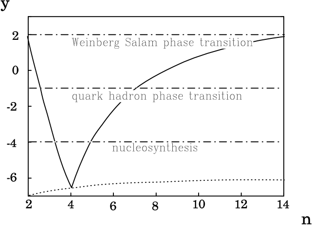
Figure 1: The energy density at the end of reheating ($\rho^{1/4}=10^{y}{\rm GeV}$) vs power of the inflaton potential $n$

In this figure the solid line and the dotted line correspond to (4.71) and (4.72), respectively, and the Bardeen parameter is well conserved in the region above these lines. This figure shows that reheating does not affect the conservation of the Bardeen parameter if it terminates before the primordial nucleosynthesis. Hence we can conclude that in all the realistic models based on chaotic inflation, the Bardeen parameter stays constant in a good accuracy during reheating. This justifies the conventional prescription relating the amplitude of adiabatic perturbations at horizon crossing in the post-Friedman stage to the value of the Bardeen parameter in the inflationary stage.

5 Discussion

In this paper we have investigated the evolution of perturbations during reheating taking account of the effect of the energy transfer from the inflaton to radiation, by replacing the inflaton field by a perfect fluid obtained by the spacetime averaging and the WKB approximation. By evaluating the amplitudes of entropy perturbations generated during reheating and their influence on the adiabatic component of perturbations, we have shown that the Bardeen parameter is well conserved during the reheating stage as well as in the inflationary stage and the post-Friedmann stage for realistic models. Though we have considered only the parametric resonance and the Born decay as the dominant reheating processes for definiteness, the conclusion holds rather generally since the arguments are insensitive to the details of the models.

Of course our analysis does not exhaust all the possible models of inflation. In particular we have only considered the case in which the inflaton is described by a single component field. Though a simple multi-component extension does not seem to change the conclusion as far as the fluid replacement of the inflaton fields during the reheating stage gives a good approximation, some subtlety may occur if scalar fields with very tiny masses coexist with the inflaton fields. For example, if there exists a scalar field which affects physical parameters controlling the reheating processes such as particle masses or coupling constants of physical particles but has no dynamical effect by itself during reheating, it may produce large entropy perturbations and affect the Bardeen parameter. In particular, as our analysis suggests, this possibility may become important if such a field affects the parameters controlling the parametric resonance processes. In such multi-component systems, entropy perturbations produced during reheating may survive after reheating and have important effects on the present universe, as discussed by Yokoyama et al. as a mechanism to generate the baryon isocurvature perturbation[13]. These problems in the multi-component extension are under investigation.

Appendix A Gauge invariant Perturbation Theory of Multi Component Systems

In this appendix, we recapitulate the basic definitions and equations of the gauge invariant perturbation theory for multicomponent systems developed in the article[5]. The purpose is twofold. The one is to explain the notations and to provide the basic equations used in the text. The other is to correct errors of the corresponding equations in [5].

The Einstein equations and the equations of motion of a perturbed multi-component system are given by

$$\tilde{G}^{\mu}_{\nu}=\kappa^{2}\tilde{T}^{\mu}_{\nu},$$ (A.1)

$$\tilde{\nabla}_{\nu}\tilde{T}^{\nu}_{(\alpha)\mu}=\tilde{Q}_{(\alpha)\mu},$$ (A.2)

where $\tilde{Q}_{(\alpha)\mu}$ represents the energy-momentum transfer term for a component $(\alpha)$, which satisfies

$$\sum_{(\alpha)}\tilde{Q}_{(\alpha)\mu}=0.$$ (A.3)

In a spatially homogeneous background with metric

$$ds^{2}=-dt^{2}+a^{2}d\sigma_{n}^{2},$$ (A.4)

where $d\sigma_{n}^{2}$ denotes a constant curvature space of dimension $n$ with a sectional curvature $K$, these equations reduce to

$$H^{2}\equiv\left({\dot{a}\over a}\right)^{2}={2\kappa^{2}\over n(n-1)}\rho-{K\over a^{2}},$$ (A.5)

$${\cal D}\rho=-nh,$$ (A.6)

$${\cal D}\rho_{\alpha}=-n(1-q_{\alpha})h_{\alpha},$$ (A.7)

Here

$${\cal D}:=a{d\over da},$$ (A.8)

$h=\rho+P$ and $h_{\alpha}=\rho_{\alpha}+P_{\alpha}$ denote the entalpies of the total system and the $(\alpha)$-component, respectively, and $q_{\alpha}$ is defined by

$$q_{\alpha}={Q_{\alpha}\over nh_{\alpha}H};\quad(Q_{(\alpha)\mu})=(Q_{\alpha},0,\cdots,0).$$ (A.9)

For scalar perturbations, the linear perturbation equations for Eq.(A.1) are written in terms of gauge-invariant quantities $\Delta$, $V$, $\Phi$, $\Psi$, $\Gamma$, and $\Pi$ representing the perturbation amplitudes of density, velocity, curvature, gravitational potential, entropy and anisotropic stress, respectively, as

$${\cal D}\Delta-nw\Delta=-C_{K}(1+w){k\over aH}V-(n-1)C_{K}w\Pi,$$ (A.10)

$${\cal D}V+V=$$

$$\quad{k\over aH}\Psi+{k\over aH}\left[{c^{2}_{S}\over 1+w}\Delta+{w\over 1+w}\Gamma\right]-{n-1\over n}{k\over aH}C_{K}{w\over 1+w}\Pi,$$ (A.11)

$$\Delta={2C_{K}\over nI_{K}}{k^{2}\over a^{2}H^{2}}\Phi,$$ (A.12)

$$(n-2)\Phi+\Psi=-\kappa^{2}{a^{2}\over k^{2}}p\Pi.$$ (A.13)

Here $w=P/\rho$, $c_{s}^{2}=\dot{P}/\dot{\rho}$ and

$$I_{K}:=1+{K\over a^{2}H^{2}},\quad C_{K}:=1-{nK\over k^{2}}.$$ (A.14)

In applications it is often more convenient to rewrite these evolution equations in terms of $\Phi$ and $\Upsilon$ defined by

$$\Upsilon:={aH\over k}V,$$ (A.15)

as

$${\cal D}\Phi+(n-2)\Phi=-{n\over 2}I_{K}(1+w)\Upsilon-{n(n-1)\over 2}({aH\over k})^{2}I_{K}w\Pi,$$ (A.16)

$${\cal D}\Upsilon+{n\over 2}I_{K}(1+w)\Upsilon-{K\over a^{2}H^{2}}\Upsilon$$

$$\quad=\Biggl{\{}-(n-2)+{c^{2}_{S}\over 1+w}{2\over n}({k\over aH})^{2}{C_{K}\over I_{K}}\Biggr{\}}\Phi+{w\over 1+w}\Gamma$$

$$\quad\quad+\Biggl{\{}-{n(n-1)\over 2}({aH\over k})^{2}wI_{K}-{n-1\over n}C_{K}{w\over 1+w}\Biggr{\}}\Pi.$$ (A.17)

On the other hand, from Eq.(A.2), the perturbation equations for each component are given by

$${\cal D}[\rho_{\alpha}\Delta_{\alpha}]+n\rho_{\alpha}\Delta_{\alpha}={n\over n-1}\kappa^{2}hh_{\alpha}{a\over kH}(V-V_{\alpha})$$

$$\qquad-C_{K}\left[h_{\alpha}{k\over aH}V_{\alpha}+(n-1)(1-q_{\alpha})P_{\alpha}\Pi_{\alpha}\right]$$

$$\qquad-nq_{\alpha}[P_{\alpha}\Gamma_{\alpha}+c^{2}_{\alpha}\rho_{\alpha}\Delta_{\alpha}]+nh_{\alpha}q_{\alpha}E_{\alpha}+n(1-q_{\alpha}){aH\over k}h_{\alpha}F_{\alpha},$$ (A.18)

$${\cal D}V_{\alpha}+V_{\alpha}={k\over aH}\Psi+{k\over aH}\left({c^{2}_{\alpha}\over 1+w_{\alpha}}\Delta_{\alpha}+{w_{\alpha}\over 1+w_{\alpha}}\Gamma_{\alpha}\right)$$

$$\qquad-{n-1\over n}{k\over aH}C_{K}{w_{\alpha}\over 1+w_{\alpha}}\Pi_{\alpha}+F_{\alpha}.$$ (A.19)

Here $E_{\alpha}$ and $F_{\alpha}$ are the gauge-invariant quantities representing the energy and the momentum transfer rate for the component $(\alpha)$ at its own rest frame. These quantities are related to the corresponding quantities at the rest frame of the total system, $E_{c\alpha}$ and $F_{c\alpha}$, by

$$E_{c\alpha}=E_{\alpha}+{a\dot{Q}_{\alpha}\over kQ_{\alpha}}(V_{\alpha}-V),$$ (A.20)

$$F_{c\alpha}=F_{\alpha}+nq_{\alpha}(V_{\alpha}-V).$$ (A.21)

These quantities must satisfy the following constraint obtained from Eq.(A.3):

$$\sum_{\alpha}Q_{\alpha}E_{c\alpha}=0,\qquad\sum_{\alpha}h_{\alpha}F_{c\alpha}=0.$$ (A.22)

Eqs.(A.10), (A.11), (A.18), (A.19) and (A.22) determine the dynamical behavior of the multicomponent system completely. However it is often more convenient to use the variables representing the relative perturbations among components defined by

$$S_{\alpha\beta}={\Delta_{c\alpha}\over 1+w_{\alpha}}-{\Delta_{c\beta}\over 1+w_{\beta}},$$ (A.23)

$$V_{\alpha\beta}=V_{\alpha}-V_{\beta},$$ (A.24)

$$\Gamma_{\alpha\beta}={w_{\alpha}\over 1+w_{\alpha}}\Gamma_{\alpha}-{w_{\beta}\over 1+w_{\beta}}\Gamma_{\beta},$$ (A.25)

$$\Pi_{\alpha\beta}={w_{\alpha}\over 1+w_{\alpha}}\Pi_{\alpha}-{w_{\beta}\over 1+w_{\beta}}\Pi_{\beta},$$ (A.26)

$$E_{\alpha\beta}=q_{\alpha}E_{c\alpha}-q_{\beta}E_{c\beta},$$ (A.27)

$$F_{\alpha\beta}=F_{c\alpha}-F_{c\beta}.$$ (A.28)

The dynamical variables for each component are written in terms of these relative variables and those for the total system as

$${\Delta_{c\alpha}\over 1+w_{\alpha}}={\Delta\over 1+w}+\sum_{\gamma}{h_{\gamma}\over h}S_{\alpha\gamma},$$ (A.29)

$$V_{\alpha}=V+\sum_{\gamma}{h_{\gamma}\over h}V_{\alpha\gamma},$$ (A.30)

$${w_{\alpha}\over 1+w_{\alpha}}\Gamma_{\alpha}={w\over 1+w}(\Gamma-\Gamma_{rel})+\sum_{\gamma}{h_{\gamma}\over h}\Gamma_{\alpha\gamma},$$ (A.31)

$${w_{\alpha}\over 1+w_{\alpha}}\Pi_{\alpha}={w\over 1+w}\Pi+\sum_{\gamma}{h_{\gamma}\over h}\Pi_{\alpha\gamma},$$ (A.32)

where $\Gamma_{\rm rel}$ is the contribution to $\Gamma$ from the relative entropy perturbations and given by

$$P\Gamma_{rel} = {1\over 2}\sum_{\alpha}\sum_{\beta}{h_{\alpha}h_{\beta}\over h}(1-q_{\alpha})(1-q_{\beta})(c^{2}_{\alpha}-c^{2}_{\beta})\times$$ (A.33)

$$\Biggl{[}{\Delta_{c\alpha}\over(1+w_{\alpha})(1-q_{\alpha})}-{\Delta_{c\beta}\over(1+w_{\beta})(1-q_{\beta})}\Biggr{]}$$

$$= {1\over 2}\sum_{\alpha}\sum_{\beta}{h_{\alpha}h_{\beta}\over h}(c^{2}_{\alpha}-c^{2}_{\beta})S_{\alpha\beta}+{1\over 1+w}{\Delta\over nH}\sum_{\alpha}c^{2}_{\alpha}Q_{\alpha}.$$

The evolution equations for these relative variables are derived as follows. First, by subtracting Eq.(A.11) from Eq.(A.19), we obtain

$${\cal D}(V_{\alpha}-V)+(V_{\alpha}-V)={k\over aH}(c^{2}_{\alpha}-c^{2}_{S}){\Delta\over 1+w}+{k\over aH}\sum_{\gamma}{h_{\gamma}\over h}c^{2}_{\alpha}S_{\alpha\gamma}$$

$$\qquad-{k\over aH}{w\over 1+w}\Gamma_{rel}+{k\over aH}\sum_{\gamma}{h_{\gamma}\over h}[\Gamma_{\alpha\gamma}-{n-1\over n}C_{K}\Pi_{\alpha\gamma}]$$

$$\qquad+F_{\alpha}+nc^{2}_{\alpha}(1-q_{\alpha})(V_{\alpha}-V).$$ (A.34)

Next from the relation

$${\Delta_{c\alpha}\over 1+w_{\alpha}}={\Delta_{\alpha}\over 1+w_{\alpha}}+{1\over 1+w_{\alpha}}{\dot{\rho}_{\alpha}\over\rho_{\alpha}}{a\over k}(V_{\alpha}-V),$$ (A.35)

Eq.(A.18), and Eq(A.34), it follows that

$${\cal D}({\Delta_{c\alpha}\over 1+w_{\alpha}})=-{k\over aH}V_{\alpha}+{nK\over kaH}V+n\{(1-q_{\alpha})c^{2}_{S}-q_{\alpha}(1+c^{2}_{\alpha})\}{\Delta\over 1+w}$$

$$\qquad+n(1-q_{\alpha}){w\over 1+w}\Gamma-nq_{\alpha}(1+c^{2}_{\alpha})\sum_{\gamma}{h_{\gamma}\over h}S_{\alpha\gamma}$$

$$\qquad-n{w_{\alpha}\over 1+w_{\alpha}}\Gamma_{\alpha}-(n-1)C_{K}(1-q_{\alpha}){w\over 1+w}\Pi+nq_{\alpha}E_{c\alpha}.$$ (A.36)

From these equations we obtain the following evolution equations for $S_{\alpha\beta}$ and $V_{\alpha\beta}$:

$${\cal D}S_{\alpha\beta}+{n\over 2}[q_{\alpha}(1+c^{2}_{\alpha})+q_{\beta}(1+c^{2}_{\beta})]S_{\alpha\beta}$$

$$\quad+{n\over 2}[q_{\alpha}(1+c^{2}_{\alpha})-q_{\beta}(1+c^{2}_{\beta})]\sum_{\gamma}{h_{\gamma}\over h}(S_{\alpha\gamma}+S_{\beta\gamma})$$

$$\quad=-{k\over aH}V_{\alpha\beta}-n\Gamma_{\alpha\beta}+nE_{\alpha\beta}$$

$$\qquad-n[(q_{\alpha}-q_{\beta})c^{2}_{S}+q_{\alpha}(1+c^{2}_{\alpha})-q_{\beta}(1+c^{2}_{\beta})]{\Delta\over 1+w}$$

$$\qquad-n(q_{\alpha}-q_{\beta}){w\over 1+w}\Gamma+(n-1)C_{K}(q_{\alpha}-q_{\beta}){w\over 1+w}\Pi,$$ (A.37)

$${\cal D}V_{\alpha\beta}+V_{\alpha\beta}-{n\over 2}[c^{2}_{\alpha}+c^{2}_{\beta}-q_{\alpha}(1+c^{2}_{\alpha})-q_{\beta}(1+c^{2}_{\beta})]V_{\alpha\beta}$$

$$\qquad-{n\over 2}[c^{2}_{\alpha}-c^{2}_{\beta}-q_{\alpha}(1+c^{2}_{\alpha})+q_{\beta}(1+c^{2}_{\beta})]\sum_{\gamma}{h_{\gamma}\over h}(V_{\alpha\gamma}+V_{\beta\gamma})$$

$$\quad={k\over aH}(c^{2}_{\alpha}-c^{2}_{\beta}){\Delta\over 1+w}+{k\over 2aH}(c^{2}_{\alpha}+c^{2}_{\beta})S_{\alpha\beta}+{k\over 2aH}(c^{2}_{\alpha}-c^{2}_{\beta})\sum_{\gamma}{h_{\gamma}\over h}(S_{\alpha\gamma}+S_{\beta\gamma})$$

$$\qquad+{k\over aH}\Gamma_{\alpha\beta}-{n-1\over n}{k\over aH}C_{K}\Pi_{\alpha\beta}+F_{\alpha\beta}.$$ (A.38)

Appendix B Upper bound on the growth rate of solutions to a first-order differential equation system

In this appendix we explain a general technique to evaluate an upper bound on the norm of the solution $X$ to the first differential equation system

$${d\over dt}\mbox{\boldmath$X$}=\mbox{\boldmath$\Omega$}(t)\mbox{\boldmath$X$}+\mbox{\boldmath$S$}(t).$$ (B.1)

Here $X$ and $S$ are $n$ column vectors, and $\Omega$ is an $n\times n$ matrix. If we define the norm of the solution $X$ by

$$\|\mbox{\boldmath$X$}\|^{2}:=\mbox{\boldmath$X$}^{\dagger}\mbox{\boldmath$X$},$$ (B.2)

it obeys the equation

$${d\over dt}(\|\mbox{\boldmath$X$}\|^{2})=\mbox{\boldmath$X$}^{\dagger}\mbox{\boldmath$\Omega$}_{H}\mbox{\boldmath$X$}+\mbox{\boldmath$S$}^{\dagger}\mbox{\boldmath$X$}+\mbox{\boldmath$X$}^{\dagger}\mbox{\boldmath$S$},$$ (B.3)

where $\mbox{\boldmath$\Omega$}_{H}$ is an hermitian matrix defined by

$$\mbox{\boldmath$\Omega$}_{H}:=\mbox{\boldmath$\Omega$}^{\dagger}+\mbox{\boldmath$\Omega$}.$$ (B.4)

The least upper bound of the right-hand side of this equation is determined by the maximum eigenvalue of $\mbox{\boldmath$\Omega$}_{H}$. However, in many cases this simple method is not practical because it gives a complicated expression. In such cases it is useful to decompose $\mbox{\boldmath$\Omega$}_{H}$ into a sum of hermitian matrices $\mbox{\boldmath$\Omega$}_{Hi}$, ($1\leq i\leq k$) as

$$\mbox{\boldmath$\Omega$}_{H}=\sum_{i=1}^{k}\mbox{\boldmath$\Omega$}_{Hi},$$ (B.5)

so that the maximum eigenvalue of each $\mbox{\boldmath$\Omega$}_{Hi}$ has a simple expression. Since the hermitian matrix $\mbox{\boldmath$\Omega$}_{Hi}$ can be diagonalized by some unitary matrix and its eigenvalues are real, we obtain

$$\mbox{\boldmath$X$}^{\dagger}\mbox{\boldmath$\Omega$}_{Hi}\mbox{\boldmath$X$}\leq\lambda_{mi}\mbox{\boldmath$X$}^{\dagger}\mbox{\boldmath$X$},$$ (B.6)

where $\lambda_{mi}$ is the largest eigenvalue of the hermitian matrix $\mbox{\boldmath$\Omega$}_{Hi}$. Hence by applying the Cauchy-Schwartz inequality

$${\rm Tr}\mbox{\boldmath$A$}^{\dagger}\mbox{\boldmath$B$}\leq({\rm Tr}\mbox{\boldmath$A$}^{\dagger}\mbox{\boldmath$A$})^{1/2}({\rm Tr}\mbox{\boldmath$B$}^{\dagger}\mbox{\boldmath$B$})^{1/2}$$ (B.7)

to Eq.(B.3), we obtain

$${d\over dt}(\|\mbox{\boldmath$X$}\|)-{\lambda_{m}\over 2}\|\mbox{\boldmath$X$}\|-\|\mbox{\boldmath$S$}\|\leq 0,$$ (B.8)

where

$$\lambda_{m}:=\sum_{i=1}^{k}\lambda_{mi}.$$ (B.9)

By integrating the inequality (B.8), we obtain

$$\|\mbox{\boldmath$X$}(t)\|\leq\exp\left(\int_{0}^{t}{\lambda_{m}(t^{\prime})\over 2}dt^{\prime}\right)\|\mbox{\boldmath$X$}(0)\|+\int_{0}^{t}dt^{\prime}\exp\left(\int_{t^{\prime}}^{t}{\lambda_{m}(t^{\prime\prime})\over 2}dt^{\prime\prime}\right)\|\mbox{\boldmath$S$}({t^{\prime}})\|.$$ (B.10)

Notice that the right-hand side of the inequality (B.10) is a monotonically increasing functional of $\lambda_{m}(s)$, $(0\leq s\leq t)$. Therefore, even if we replace $\lambda_{m}$ by a larger value, the inequality (B.10) still holds.

In the case $\lambda_{m}(t)<0$ and $|\lambda_{m}(t)|\gg 1$, we can derive a simpler estimate on $\|\mbox{\boldmath$X$}\|$. To see this, let us introduce $x(t^{\prime})$ defined by

$$x(t^{\prime}):=-\int_{t^{\prime}}^{t}\lambda_{m}(t^{\prime\prime})dt^{\prime\prime}.$$ (B.11)

Then the second term in the right-hand side of Eq.(B.10 ) is written as

$$\int_{0}^{t}dt^{\prime}\exp\left({1\over 2}\int_{t^{\prime}}^{t}\lambda_{m}(t^{\prime\prime})dt^{\prime\prime}\right)\|\mbox{\boldmath$S$}(t^{\prime})\|=\int_{0}^{\Lambda}dx\exp\left(-{1\over 2}x\right){\|\mbox{\boldmath$S$}\|_{x}\over|\lambda_{m}|_{x}},$$ (B.12)

where

$$\Lambda=\int_{0}^{t}|\lambda_{m}(t^{\prime})|dt^{\prime}.$$ (B.13)

Hence, if $\|\mbox{\boldmath$S$}\|/|\lambda_{m}|$ is a slowly varying function of $t$ and $\Lambda\gg 1$, we obtain

$$\int_{0}^{t}dt^{\prime}\exp(\int_{t^{\prime}}^{t}{\lambda_{m}(t^{\prime\prime})\over 2}dt^{\prime\prime})\|\mbox{\boldmath$S$}({t^{\prime}})\|\leq{\rm O}\!\left(\|\mbox{\boldmath$S$}(t)\|\over|\lambda_{m}(t)|\right).$$ (B.14)

References

- [1] S.W. Hawking, Phys. Lett. B 115, 295–297 (1982); A.G. Guth and S.-Y. Pi, Phys. Rev. Lett. 49, 1110–1113 (1982); A.A. Starobinsky, Phys. Lett. B 117, 175 (1982).
- [2] J.M. Bardeen, P.J. Steinhardt, and M.S. Turner, Phys. Rev. D 28, 679–693 (1983).
- [3] J.A. Friemann and M.S. Turner, Phys. Rev. D 30, 265–271 (1984).
- [4] R. Brandenberger and R. Kahn, Phys. Rev. D 29, 2172–2190 (1984).
- [5] H. Kodama and M. Sasaki, Prog. Theor. Phys. Suppl. 78, 1 (1984).
- [6] J. Traschen and R. Brandenberger, Phys. Rev. D42, 2491 (1990).
- [7] L. Kofman, A. Linde and A. A. Starobinsky, Phys. Rev. Lett. 73, 3195 (1994).
- [8] Y. Shtanov, J. Traschen and R. Brandenberger, Phys. Rev. D51, 5438 (1995).
- [9] M. Yoshimura, Prog. Theor. Phys. 94, 873, (1995)
- [10] H. Kodama, and T. Hamazaki gr-qc/9608022,YITP-96-28,KUNS 1406
- [11] V. F. Mukhanov, H. A. Feldman and R. H. Brandenberger, Physics Reports 215, 203 (1992)
- [12] S. Yu.Khlebnikov and I. I. Tkachev, Phys. Rev. Lett. 77, 219 (1996)
- [13] M. Yoshimura, Phys. Rev. Lett. 51, 439, (1983); M. Sasaki and J. Yokoyama, Phys. Rev. D44, 970 (1991).