Colliding black holes: how far can the close approximation go?

Abstract

We study the head-on collision of two equal-mass momentarily stationary black holes, using black hole perturbation theory up to second order. Compared to first-order results, this significantly improves agreement with numerically computed waveforms and energy. Much more important, second-order results correctly indicate the range of validity of perturbation theory. This use of second-order, to provide “error bars,” makes perturbation theory a viable tool for providing benchmarks for numerical relativity in more generic collisions and, in some range of collision parameters, for supplying waveform templates for gravitational wave detection.

The head-on collision of two momentarily stationary black holes has become a classic problem in general relativity. This is in part due to the fact that it is simple, when compared to more generic collisions, yet can be used as a testbed for ideas that will later be applied in the astrophysically more relevant case of an inspiralling coalescence. The problem is far from academic. The near advent of gravitational wave detectors, like the LIGO or VIRGO projects, that should be able to measure gravitational radiation from colliding black holes, is a strong motivation for obtaining accurate waveform templates as soon as possible. Because one expects that most of the signal will be hidden by noise in a gravitational wave detector, knowing the templates accurately can mean the difference between detecting and not detecting [1] gravitational waves.

An important approach to the problem has been with numerical relativity, pioneered by Smarr [2] in the 70’s. The state of the art in these techniques yields a fairly accurate computation of radiated energies and waveforms for head-on (axisymmetric) coalescences[3], but further development of numerical relativity will be needed to generalize computations to cases with less symmetry. Recently [4, 5], perturbative techniques applied to this problem were found to give remarkably good results when the holes were initially close. By treating the collision of close black holes as the dynamics of a single distorted black hole, one can use the well understood machinery of black hole perturbation theory to treat the problem. Better yet, generalization of these techniques to collisions without axisymmetry entails only minor modifications.

A key missing element in perturbative close-approximation calculations is that one cannot tell a priori over what range it is valid. (How close is “close enough”?) The main point of this article is to show that this missing element is provided by second-order perturbation theory, which has recently been developed [6], largely for this purpose. A higher-order calculation is characterized by a number of interesting technical issues (such as gauge choices of different order), and by considerable complexity. Here we want only briefly to describe the nature of the computation, and to argue the importance of the first results. We initially specialize to the details (e.g., even-parity only) of a head-on collision of two non-spinning equal-mass holes starting with Misner[7] initial data. This is done for definiteness in the description, and because this is the case which can most thoroughly be compared with the numerical results.

The perturbation calculation starts with an expansion of the metric, in terms of a perturbation parameter $\epsilon$, in the form $g_{\mu\nu}=g_{\mu\nu}^{\rm Schw}+\epsilon h_{\mu\nu}^{(1)}+\epsilon^{2}h_{\mu\nu}^{(2)}+{\cal O}(\epsilon^{2})$, where $g_{\mu\nu}^{\rm Schw}$ is the usual Schwarzschild metric, for a spacetime of mass $M$. Work on perturbation theory, more than twenty years ago, showed that for even-parity perturbations all the physical information in each $\ell$-pole of the first-order perturbations $h_{\mu\nu}^{(1)}$ can be encoded into a single “Zerilli function” $\psi^{(1)}_{\ell}$ that is a combination of the $h_{\mu\nu}^{(1)}$ and their derivatives[8, 9]. This function satisfies the Zerilli equation, a simple, linear wave-like equation. If we construct essentially the same combination of $h_{\mu\nu}^{(2)}$ to form a second-order Zerilli function $\psi^{(2)}_{\ell}$, the Einstein vacuum equations, to second order in $\epsilon$, guarantee that $\psi^{(2)}$ will satisfy a wave equation

$$-\partial_{t}^{2}\psi^{(2)}_{\ell}+\partial_{r^{*}}^{2}\psi^{(2)}_{\ell}+V_{\ell}(r)\psi^{(2)}_{\ell}={\cal S}_{\ell}\ ,$$ (1)

which differs from the usual Zerilli equation only in the presence of a nonzero “source” term on the right[10]. In this equation, $r^{*}\equiv r+2M\ln(r/2M-1)$ and $V_{\ell}(r)$ is given, e.g., in [8, 9]. The new feature for second-order, the source term ${\cal S}_{\ell}$, is a quadratic function of $\psi^{(1)}_{\ell}$. In the case of the head-on collision, though not more generally, it turns out that only the $\ell=2$ first-order terms contribute to the quadrupole source ${\cal S}_{2}$. For this case the source is explicitly given in [6].

There are two ways in which $\psi^{(2)}_{\ell}$ is not exactly the same combination of the $h_{\mu\nu}^{(2)}$, as $\psi^{(1)}_{\ell}$ is of the $h_{\mu\nu}^{(1)}$. First, for technical reasons[6], $\psi^{(2)}_{\ell}$ is actually equivalent to the time derivative of the second-order Zerilli function. Second, $\psi^{(2)}_{\ell}$ is not unique; one can redefine it up to terms quadratic in the first-order perturbations. The choice made in [6] ensures that the source term is such that it yields a well behaved $\psi^{(2)}_{2}$ in the radiation zone. (Here $\psi^{(2)}_{2}$ corresponds to $\chi$ in the notation of [6].)

For the head-on collision problem, the perturbation expansion parameter $\epsilon$ is a measure of the initial separation of the holes. The particular choice we make is the parameter denoted $\kappa_{2}$ in Ref. [4] that occurs rather naturally in the description of the problem. It is straightforward to expand the Misner initial data in this parameter and to find $h_{\mu\nu}^{(1)}$ and $h_{\mu\nu}^{(2)}$, from which we derive the initial conditions for the dominant $\ell=2$ perturbations,

$$\psi^{(1)}_{2}|_{t=0} = {128\over 3}{M^{3}r\over(2r+3M)}{[7\sqrt{r}+5\sqrt{r-2M}]\over[\sqrt{r}+\sqrt{r-2M}]^{5}}$$ (2)

$$\partial_{t}\psi^{(1)}_{2}|_{t=0} = 0$$ (3)

$$\psi^{(2)}_{2}|_{t=0} = -{131072\over 7}{M^{6}\over r(\sqrt{r}+\sqrt{r-2M})^{10}}$$ (4)

$$\partial_{t}\psi^{(2)}_{2}|_{t=0} = {16384\over 7}{M^{6}[5(r-M)\sqrt{r-2M}+19\sqrt{r}(r-2M)]\over(\sqrt{r}+\sqrt{r-2M})^{10}(2r+3M)}\ .$$ (5)

(The surprising nonzero time derivative in (5) arises partly because $\psi^{(2)}_{2}$ is actually the time derivative of the second-order Zerilli function, and partly due to the quadratic terms that were added to $\psi^{(2)}_{2}$ to make it well behaved in the radiation zone [11].) The solution for $\psi^{(1)}_{2}$, and therefore the source term for (1), is known numerically from the solution to the first-order problem[4]. This source and the initial data of (4) and (5) complete the specification of the problem defined by (1).

With the solution of that problem for $\psi^{(1)}_{2}$, from a simple finite differencing scheme (and with $\psi^{(1)}_{1}$ from the first-order solution), the radiated power is found from

$${\rm Power}={3\over 10}\left\{\epsilon{\partial\psi^{(1)}_{2}\over\partial t}+\epsilon^{2}\left[\psi^{(2)}_{2}+{1\over 7}{\partial\over\partial t}\left(\psi^{(1)}_{2}{\partial\psi^{(1)}_{2}\over\partial t}\right)\right]\right\}^{2}\ ,$$ (6)

and the energy radiated is the time integral of this expression. The expression in brackets $\left\{\right\}$ is proportional to our second-order radiation wavefunction, and omits yet-higher-order corrections. In applying (6), it would be inconsistent to keep the terms of order $\epsilon^{4}$, which are of higher order than omitted terms, so we compute energy only to order $\epsilon^{3}$.

FIG. 1.: The total radiated energy in a black hole collision as a fraction of the spacetime mass $M$ for different values of the initial separation. The upper scale is in units of $L/m$, where $m$ is the mass of each individual hole (inferred from the minimal area of the throat for each hole); the bottom scale is in the parameter $\mu_{0}$ that appears in the Misner data. The dotted curve is the first-order result and the solid curve the result up to second order. For $\mu_{0}\approx 2.2$ the second-order corrections are as large as the first order result. The numerical results (with error bars) correspond to the NCSA simulations of Ref. [3].

Figure 1 shows the energy results (to order $\epsilon^{3}$) as a function of the Misner[7] parameter $\mu_{0}$. This figure compares these second-order results with first-order results and with those of numerical relativity, and illustrates the point we wish to emphasize. If we had only the first-order calculations, we would know that the predictions at very large separation parameter $\mu_{0}$ were unreasonable, but we would not know how small $\mu_{0}$ must be for the results to be reasonably accurate. By comparing the first-order prediction with that of the second-order computation, we can infer that perturbation theory is applicable up to $\mu_{0}$ of order 1.8 or so. (The actual cutoff would depend on what level of accuracy one demands.) In the case of the head-on collision from Misner data, this prediction is subject to verification by comparison with the results of numerical relativity. Figure 1 clearly shows that the prediction is correct; perturbation theory is valid (i.e., agrees with numerical relativity results) up to around $\mu_{0}=1.8$. Second-order calculations do in this case provide “error bars” for perturbation calculations. There is nothing specific about the head-on problem that favors this outcome, and it is reasonable to infer that that second-order results will provide the same “error bars” in generic coalescences.

A mild caveat hangs over the application of this method to other cases. There is no unique division of perturbations into orders[12]. If, for example, one knew the exact radiated energy for the head-on collision, for all values of $\mu_{0}$, one could define a new expansion parameter $\epsilon$ that depends on $\mu_{0}$ in such a way that first-order perturbation theory would be exact! More worrisome, in any perturbation problem one could define an $\epsilon$ for which the first-order energy is not exact, but for which the second-order perturbations are zero. The “error bars” provided by these second-order perturbations would be wildly misleading[13]. Such cases keep our method of error-bar determination from being rigorous, but are a problem more in principle than in practice. Anomalous behavior of an order of perturbations arises only in atypical circumstances, usually when one contrives to arrive at just such an atypical result. For a “generic” perturbation parameter one expects the second-order error-bar method to be just as useful as in Fig. 1.

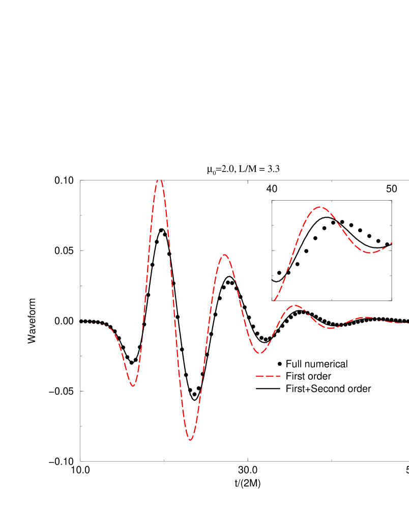
FIG. 2.: Waveforms for $\mu_{0}=2$. Shown are the waveform for time derivative of the first-order Zerilli function and that waveform with the second-order correction added. This is compared with the equivalent waveform from numerical relativity. We see a significant improvement due to the use of second-order perturbation theory, even for this case where the separation of the two black holes is $L/M\approx 3.3$. The inset shows late oscillations. The period of the numerical relativity result for these oscillations becomes larger than the quasinormal period and is thought to be a numerical artifact [5]. The second-order correct curve then is probably more accurate in this region. The full numerical data sets have higher resolution than the one depicted, we have omitted some data points for visual clarity.

A secondary advantage of second-order computation is that it can give improved accuracy of results. The difference between first-order results and second-order-correct results is, of course, significant only for cases in which perturbation theory is marginally applicable. But it is just these cases for which the radiation is strongest and which will typically be of greatest interest for comparison with numerical relativity, or for considerations of detector design. In Fig. 2 we show a comparison of waveforms for the marginal case of $\mu_{0}=2$, corresponding to an initial proper distance $L=3.3M$ between the throats. At this separation there is no single all-encompassing horizon surrounding both throats, so the assumptions of the close limit approximation are violated. As expected, the first-order result shows significant disagreement with the numerical relativity result, but the result of our second-order computation is a waveform in remarkably good agreement with the numerical relativity result.

The success is not only remarkable, it is at first somewhat puzzling. The waveform for second-order theory has an amplitude that is at most around 10% larger than the numerical relativity waveform, implying that the second-order result for radiated energy should be around 20% larger than that from numerical relativity. In Fig. 1, however, the second-order energy is about half the result of numerical relativity at $\mu_{0}=2$. The explanation of this brings out an interesting point about the computations. If we take the second-order waveform of Fig. 2, square it, multiply it by the correct factor and integrate, we calculate an energy which is, as it must be, about 20% larger than that from numerical relativity (i.e., the result of the same operations on the numerical relativity waveform of Fig. 2). But this procedure for computing second-order energy includes the formally disallowed $\epsilon^{4}$ terms in (6). The success of this formally inconsistent procedure suggests that the omitted terms in (6) are small, so that the effect of omitting them is unimportant. We must keep in mind that for a marginal case like $\mu_{0}=2$ the expansion parameter is of order unity, so that “order in $\epsilon$” is not necessarily the critical factor in the importance of a term. The omitted terms in (6) turn out to be the result of a nonlinear mixing of $\ell=2$ and $\ell=4$ contributions. The $\ell=4$ contribution for the problem is small, quite aside from the fact that it is higher order in $\epsilon$. [See Fig. 12 of Ref. [5]; at $\mu_{0}=2$, the $\ell=4$ energy is three orders of magnitude smaller than the $\ell=2$ energy.] Our higher-order waveforms are more accurate than are implied by a comparison of first-order and second-order-correct energies, but this fact may be peculiar to the specific case of initial Misner data, and not applicable to more general black hole collisions.

It is the study of more general collisions to which this work is directed. We have shown that we have a practical and reliable (though not rigorous) index of the accuracy of perturbation theory, and hence the basis for a consistent investigation of collisions that are of interest as sources of detectable gravitational waves. With estimates of accuracy established by higher-order calculations, perturbation theory will give waveforms and energies that will check numerical relativity codes; that can help in exploring the parameter space of collisions for those cases of interest for greater numerical work; that can in some cases provide guidelines for development of details of detection schemes. Work is already underway on the application of this technique to the head-on collision of initially moving and spinning holes, and has started on the modifications that are needed when the final hole is rapidly rotating.

We wish to thank Peter Anninos for help in providing the full numerical results from the NCSA group. This work was supported in part by grants NSF-INT-9512894, NSF-PHY-9423950, NSF-PHY-9507719, by funds of the University of Córdoba, the University of Utah, the Pennsylvania State University and its Office for Minority Faculty Development, and the Eberly Family Research Fund at Penn State. We also acknowledge support of CONICET and CONICOR (Argentina). JP also acknowledges support from the Alfred P. Sloan Foundation through an Alfred P. Sloan fellowship.

REFERENCES

- [1] L. S. Finn, Phys. Rev. D46, 5236 (1992).
- [2] L. Smarr, in Sources of gravitational radiation, L. Smarr, editor, Cambridge University Press, Cambridge, England, p. 245 (1979).
- [3] P. Anninos, D. Hobill, E. Seidel, L. Smarr, W.-M. Suen, Phys. Rev. Lett. 71, 2851 (1993).
- [4] R. Price, J. Pullin, Phys. Rev. Lett. 72, 3297 (1994).
- [5] P. Anninos, E. Seidel, R. Price, J. Pullin, W.-M. Suen, Phys. Rev. D52, 4462 (1995).
- [6] R. Gleiser, O. Nicasio, R. Price, J. Pullin, “Second order perturbations of a Schwarzschild black hole”, gr-qc/9510049.
- [7] C. Misner, Phys. Rev. D118, 1110 (1960).
- [8] F. Zerilli, Phys. Rev. Lett. 24, 737 (1970).
- [9] V. Moncrief, Ann. Phys. (NY) 88, 323 (1974).
- [10] This feature of second-order perturbation theory is pointed out in, e.g.: K. Tomita, Prog. Theor. Phys. 52, 1188 (1974); C. T. Cunningham, R. H. Price, and V. Moncrief, Astrophys. J 236, 674 (1980).
- [11] The transverse-traceless metric perturbation in the radiation zone is given by the expression within the curly braces in equation (6).
- [12] A. Abrahams, R. Price, Phys. Rev. D53, 1963 (1996).
- [13] Changing orders of perturbation in this way is guaranteed only for a single function of the perturbation parameter (in our case, the energy as a function of separation). The different sorts of information contained in a waveform (phases, relative amplitudes of different peaks, etc.) may not all be subject to simultaneous manipulation in this way. Comparing first-order wave forms with second-order-correct waveforms, therefore, may give a more certain determination of the valid range of perturbation theory, especially in cases where the waveforms have richer detail than for head-on collisions.