Detecting relic gravitational radiation from string cosmology with LIGO

Abstract

A characteristic spectrum of relic gravitational radiation is produced by a period of “stringy inflation” in the early universe. This spectrum is unusual, because the energy-density rises rapidly with frequency. We show that correlation experiments with the two gravitational wave detectors being built for the Laser Interferometric Gravitational Observatory (LIGO) could detect this relic radiation, for certain ranges of the parameters that characterize the underlying string cosmology model.

Preprint Numbers: WISC-MILW-96-TH-34,BGU-PH-96/09

I INTRODUCTION

Because the gravitational interaction is so weak, a stochastic background of gravitational radiation (the graviton background) decouples from the matter in the universe at very early times. For this reason, the stochastic background of gravitational radiation, which is in principle observable at the present time, carries with it a picture of the state of the universe at very early times, when energy densities and temperatures were very large.

The most interesting features of string theory are associated with its behavior at very high energies, near the Planck scale. Such high energies are unobtainable in present-day laboratories, and are unlikely to be reached for quite some time. They were, however, available during the very early history of the universe, so string theory can be probed by the predictions which it makes about that epoch.

Recent work has shown how the early universe might behave, if superstring theories are a correct description of nature [1, 2]. One of the robust predictions of this “string cosmology” is that our present-day universe would contain a stochastic background of gravitational radiation [3, 4], with a spectrum which is quite different than that predicted by many other early-universe cosmological models [5, 6, 7]. In particular, the spectrum of gravitational waves predicted by string cosmology has rising amplitude with increasing frequency. This means that the radiation might have large enough amplitude to be observable by ground-based gravity-wave detectors, which operate at frequencies above $\approx 10\>\rm Hz$. This also allows the spectrum to be consistent with observational bounds arising at $10^{-18}\>\rm Hz$ from observations of the Cosmic Background Radiation and at $10^{-8}\>\rm Hz$ from observation of millisecond pulsar timing residuals.

In this short paper, we examine the spectrum of radiation produced by string cosmology, and determine the region of parameter space for which this radiation would be observable by the (initial and advanced versions of the) LIGO detectors [8].

II Stochastic background in string cosmology

In models of string cosmology [3], the universe passes through two early inflationary stages. The first of these is called the “dilaton-driven” period and the second is the “string” phase. Each of these stages produces stochastic gravitational radiation; the contribution of the dilaton-driven phase is currently better understood than that of the string phase.

In order to describe the background of gravitational radiation, it is conventional to use a spectral function $\Omega_{\rm GW}(f)$ which is determined by the energy density of the stochastic gravitational waves. This function of frequency is defined by

$$\Omega_{\rm GW}(f)={1\over\rho_{\rm critical}}{d\rho_{\rm GW}\over d\ln f}.$$ (1)

Here $d\rho_{\rm GW}$ is the (present-day) energy density in stochastic gravitational waves in the frequency range $d\ln f$, and $\rho_{\rm critical}$ is the critical energy-density required to just close the universe. This is given by

$$\rho_{\rm critical}={3c^{2}H_{0}^{2}\over 8\pi G}\approx 1.6\times 10^{-8}{\rm h}_{100}^{2}\rm\>ergs/cm^{3},$$ (2)

where the Hubble expansion rate $H_{0}$ is the rate at which our universe is currently expanding,

$$H_{0}={\rm h}_{100}\>100\>{\rm Km\over sec-Mpc}=3.2\times 10^{-18}{\rm h}_{100}{\rm 1\over sec}.$$ (3)

Because $H_{0}$ is not known exactly, it is defined in terms of a dimensionless parameter ${\rm h}_{100}$ which is believed to lie in the range $1/2<{\rm h}_{100}<1$.

The spectrum of gravitational radiation produced in the dilaton-driven and string phase was discussed in [3]. In the simplest model, which we will use in this paper, it depends upon four parameters. The first pair of these are the frequency ${f_{\rm S}}$ and the fractional energy density $\Omega^{\rm S}_{\rm GW}$ produced at the end of the dilaton-driven phase. The second pair of parameters are the maximal frequency $f_{1}$ above which gravitational radiation is not produced and the maximum fractional energy density $\Omega^{\rm max}_{GW}$, which occurs at that frequency. This is illustrated in Fig. 1.

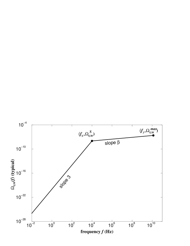
FIG. 1.: A string cosmology gravitational wave power spectrum. The part of the spectrum with slope 3 below frequency ${f_{\rm S}}$ is produced during the dilaton-driven phase, and the part of the spectrum above that frequency is produced during the string phase.

An approximate form for the spectrum is [9]

$$\Omega_{\rm GW}(f)=\cases{{\Omega^{\rm S}_{\rm GW}(f/{f_{\rm S}})^{3}}&{ $f<{f_{\rm S}}$}\cr&\cr{\Omega^{\rm S}_{\rm GW}(f/{f_{\rm S}})^{\beta}}&${f_{\rm S}}<f<f_{1}$\cr&\cr{0}&$f_{1}<f$}$$ (4)

where

$$\beta=\frac{\log\left[\Omega_{\rm GW}^{\rm max}/\Omega^{\rm S}_{\rm GW}\right]}{\log\left[f_{1}/{f_{\rm S}}\right]}$$

is the logarithmic slope of the spectrum produced in the string phase.

If we assume that there is no late entropy production and make reasonable choices for the number of effective degrees of freedom, then two of the four parameters may be determined in terms of the Hubble parameter $H_{\rm r}$ at the onset of radiation domination immediately following the string phase of expansion [10],

$$f_{1}=1.3\times 10^{10}\>{\rm Hz}\left({H_{\rm r}\over 5\times 10^{17}\>{\rm GeV}}\right)^{1/2}$$ (5)

and

$$\Omega_{\rm GW}^{\rm max}=1\times 10^{-7}{\rm h}_{100}^{-2}\left({H_{\rm r}\over 5\times 10^{17}\>{\rm GeV}}\right)^{2}.$$ (6)

More complicated models and spectra were discussed in [11, 12, 13].

The ratios $\left(\Omega^{\rm S}_{\rm GW}/\Omega_{\rm GW}^{\rm max}\right)$ and $\left(f_{\rm S}/f_{1}\right)$ are determined by the basic physical parameters of string cosmology models, the values of the Hubble parameter and the string coupling parameter at the end of the dilaton-driven phase and the onset of the string phase [3, 9, 14].

III Detecting a stochastic background

A number of authors [15, 16, 17, 7] have shown how one can use a network of two or more gravitational wave antennae to detect a stochastic background of gravitational radiation. The basic idea is to correlate the signals from separated detectors, and to search for a correlated strain produced by the gravitational-wave background, which is buried in the intrinsic instrumental noise. It has been shown by these authors that after correlating signals for time $T$ (we take $T=10^{7}\>{\rm sec}=3\>{\rm months}$) the ratio of “Signal” to “Noise” (squared) is given by an integral over frequency $f$:

$$\left({S\over N}\right)^{2}={9H_{0}^{4}\over 50\pi^{4}}T\int_{0}^{\infty}df\>{\gamma^{2}(f)\Omega_{\rm GW}^{2}(f)\over f^{6}P_{1}(f)P_{2}(f)}.$$ (7)

FIG. 2.: The predicted noise power spectra of the initial and advanced LIGO detectors. The horizontal axis is $\rm log_{10}$ of frequency $f$, in Hz. The vertical axis shows $\rm log_{10}(P(f)/sec)^{1/2}$, or strain per root Hz. These noise power spectra are the published design goals. The bumps appearing in the low-frequency part of the advanced LIGO noise curve are obtained by folding measured seismic noise data with the predicted transfer function of the seismic isolation (stack) system.

In order to detect a stochastic background with $90\%$ confidence the ratio $S\over N$ needs to be at least $1.65$. In this equation, several different functions appear, which we now define. The instrument noise in the detectors is described by the one-sided noise power spectral densities $P_{i}(f)$. The LIGO project is building two identical detectors, one in Hanford Washington and one in Livingston Louisiana, which we will refer to as the “initial” detectors. After several years of operation, these detectors will be upgraded to so-called “advanced” detectors. Since the two detectors are identical in design, $P_{1}(f)=P_{2}(f)$. The design goals for the detectors specify these functions [8]. They are shown in Fig. 2. The next quantity which appears is the overlap reduction function $\gamma(f)$. This function is determined by the relative locations and orientations of the arms of the two detectors, and is identical for both the initial and advanced LIGO detectors. For the pair of LIGO detectors

$$\gamma(f)=-0.124842\>j_{0}(x)-2.90014\>{{j_{1}(x)}\over x}+3.00837\>{{j_{2}(x)}\over{{x^{2}}}},$$ (8)

where the $j_{i}$ are spherical Bessel functions. The dimensionless frequency variable is $x=2\pi f\tau$ with $\tau=10.00\>\rm msec$ being the light-travel-time between the two LIGO detector sites. This function is shown in Fig. 3.

FIG. 3.: The overlap reduction function $\gamma(f)$ for the two LIGO detector sites. (The horizontal axis of the left-hand graph is linear, while that of the right-hand graph is $\rm log_{10}$.) The overlap reduction function shows how the correlation of the detector pair to an unpolarized stochastic background falls off with frequency. The overlap reduction function has its first zero at 64 Hz, and falls off rapidly at higher frequencies.

Equation (7) allows us to assess the detectability (using initial or advanced LIGO) of any particular stochastic background $\Omega_{\rm GW}(f)$.

IV Detecting a string cosmology stochastic background

Making use of the prediction from string cosmology, we may use equation (7) to assess the detectability of this stochastic background. For any given set of parameters we may numerically evaluate the signal to noise ratio $S/N$; if this value is greater than $1.65$ then with at least 90% confidence, the background can be detected by LIGO. The regions of detectability in parameter space are shown in Fig. 4 for the initial LIGO detectors, and in Fig. 5 for the advanced LIGO detectors. For these figures we have assumed ${\rm h}_{100}=0.65$ and $H_{\rm r}=5\times 10^{17}\>{\rm GeV}$. The observable regions for different values of these parameters can be obtained by simple scaling of the presented results.

At the moment, the most restrictive observational constraint on the spectral parameters comes from the standard model of big-bang nucleosynthesis (NS) [18]. This restricts the total energy density in gravitons to less than that of approximately one massless degree of freedom in thermal equilibrium. This bound implies that

$$\int\Omega_{\rm GW}(f)d\ln f=\Omega_{\rm GW}^{\rm S}\left[\frac{1}{3}+\frac{1}{\beta}\left(\left(f_{1}/f_{\rm S}\right)^{\beta}-1\right)\right]<0.7\times 10^{-5}{\rm h}^{-2}_{100}.$$ (9)

where we have assumed an allowed $N_{\nu}=4$ at NS, and have substituted in the spectrum (4). This bound is shown on Figs. 4,5. We also show the weaker “Dilaton Only” bound, assuming NO stochastic background is produced during the (more poorly-understood) string phase of expansion:

$$\Omega_{\rm GW}^{\rm S}<2.1\times 10^{-5}{\rm h}^{-2}_{100}.$$ (10)

This is obtained by setting $f_{1}=f_{\rm S}$ in the previous equation, i.e. assuming that $\Omega_{\rm GW}$ vanishes for ${f_{\rm S}}<f<f_{1}$. We note that if the “Dilaton + String” spectrum is correct, then the NS bounds rule out any hopes of observation by initial LIGO. On the other hand, in the “Dilaton Only” case, a detectable background is not ruled out by NS bounds; it would be observable if the spectral peak falls into the detection bandpass between 50 and 200 Hz (figure 7 of [7]).

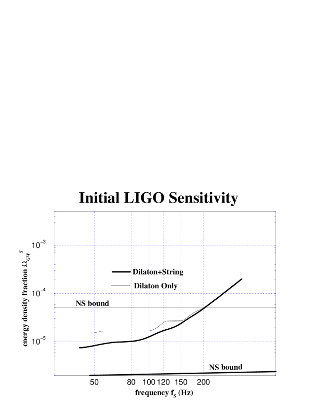
FIG. 4.: Shown is the region in parameter space for which the gravitational wave stochastic background is observable by the initial LIGO detector. The region above and to the left of the curves is where the signal to noise ratio exceeds 1.65 and the background is observable with 90% confidence. The two curves are indistinguishable above $f_{\rm S}=200\>\rm Hz$. The two lines labeled “NS bound” are nucleosynthesis bounds. The allowed region is below each line. Note that the Dilaton+String line lies below the 90% confidence curve.

Because the function $\left(\frac{\gamma(f)}{P(f)}\right)^{2}$ decays rapidly at high and low frequencies, the asymptotic behavior of the 90% confidence contours for the advanced LIGO detector in the high and low $f_{\rm S}$ regions can be estimated analytically as follows

$$(\Omega_{\rm GW}^{\rm S})_{90\%}=7.4\times 10^{-10}{\rm h}_{100}^{-2}(f_{\rm S}/100\>{\rm Hz})^{3},\ \ \ \ f_{\rm S}\raise 1.72218pt\hbox{$>$}\kern-6.99997pt\lower 2.6694pt\hbox{$\sim$}100\>{\rm Hz}$$ (11)

$$(\Omega_{\rm GW}^{\rm S})_{90\%}=2.6\times 10^{-11}\ {\rm h}_{100}^{-2}\ (f_{\rm S}/20\>{\rm Hz})^{0.4},\ \ \ \ f_{\rm S}\raise 1.72218pt\hbox{$<$}\kern-8.00003pt\lower 2.6694pt\hbox{$\sim$}20\>{\rm Hz}$$ (12)

Similar estimates may be obtained for the initial LIGO detector.

V Conclusion

In this short paper, we have shown how data from the the initial and advanced versions of LIGO will be able to constrain string cosmology models of the early universe. In principle, this might also constrain the fundamental parameters of superstring theory. The initial LIGO is sensitive only to a narrow region of parameter space and is only marginally above the required sensitivity, while the advanced LIGO detector has far better detection possibilities. The simultaneous operation of other types of gravitational wave detectors which operate at higher frequencies, such as bar and resonant designs, ought to provide additional increase in sensitivity and therefore further constrain the parameter space.

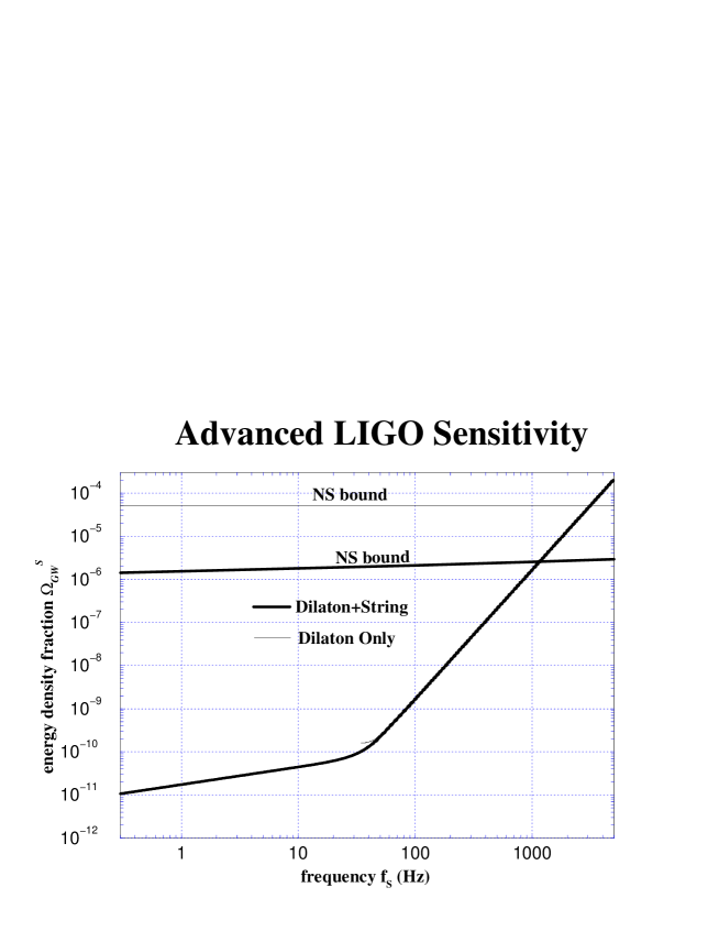
FIG. 5.: This graph is identical to the previous one, but for the advanced LIGO detector. The observable region of parameter space is above and to the left of the curves. The two curves are indistinguishable above $f_{\rm S}=50\>\rm Hz$.

- [1] G. Veneziano, Phys. Lett. B265 (1991) 287.
- [2] M. Gasperini and G. Veneziano, Astropart. Phys. 1 (1993) 317; Mod. Phys. Lett. A8 (1993) 3701.
- [3] R. Brustein, M. Gasperini, M. Giovannini and G. Veneziano Phys. Lett. B361 (1995) 45.
- [4] M. Gasperini and M. Giovannini, Phys. Rev. D47 (1993) 1519.
- [5] L.P. Grishchuk, Sov. Phys. JETP 40 (1975) 409.
- [6] M. S. Turner, Detectability of inflation produced gravitational waves, preprint Fermilab-pub-96-169-A (astro-ph/9607066).
- [7] B. Allen, The stochastic gravity-wave background: sources and detection, in Proceedings of the Les Houches School on Astrophysical Sources of Gravitational Radiation, Springer-Verlag, 1996.
- [8] A. Abramovici, et. al., Science 256 (1992) 325.
- [9] R. Brustein, Spectrum of cosmic gravitational wave background, preprint BGU-PH-96-08 (hep-th/9604159).
- [10] R. Brustein, M. Gasperini and G. Veneziano, Peak and endpoint of the relic graviton background in string cosmology, preprint CERN-TH-96-37 (hep-th/9604084).
- [11] M. Gasperini, Relic gravitons from the pre-big-bang: what we know and what we do not know, preprint CERN-TH-96-186 (hep-th/9607146).
- [12] A. Buonanno, M. Maggiore and C. Ungarelli, Spectrum of relic gravitational waves in string cosmology, preprint IFUP-TH-25-96 (gr-qc/9605072).
- [13] M. Galluccio, M. Litterio and F. Occhionero, Graviton spectra in string cosmology, Rome preprint (gr-qc/9608007).
- [14] G. Veneziano, String cosmology and relic gravitational radiation, preprint CERN-TH-96-37 (hep-th/9606119).
- [15] P. Michelson, Mon. Not. Roy. Astron. Soc. 227 (1987) 933.
- [16] N. Christensen, Phys. Rev. D46 (1992) 5250.
- [17] E. Flanagan, Phys. Rev. D48 (1993) 2389. Note that the second term on the right hand side of equation (b6) should read rather than , and that the sliding delay function shown in Figure 2 on page 2394 is incorrect.
- [18] V. F. Schwartzmann, JETP Lett. 9 (1969) 184; T. Walker et al., Ap. J. 376 (1991) 51.