A left-handed simplicial action for euclidean general relativity

Abstract

An action for simplicial euclidean general relativity involving only left-handed fields is presented. The simplicial theory is shown to converge to continuum general relativity in the Plebanski formulation as the simplicial complex is refined. This contrasts with the Regge model for which M. Miller and Brewin have shown that the full field equations are much more restrictive than Einstein’s in the continuum limit. The action and field equations of the proposed model are also significantly simpler then those of the Regge model when written directly in terms of their fundamental variables.

An entirely analogous hypercubic lattice theory, which approximates Plebanski’s form of general relativity is also presented.

1 Introduction

It has been known for some time that in general relativity (GR) the gravitational field can be represented entirely by left-handed fields, i.e. connections and tensors that transform only under the left-handed, or self-dual subgroup of the frame rotation group.

The present paper presents a simplicial model of GR with an internal $SU(2)$ gauge symmetry which, at least in the continuum limit, corresponds to the left handed frame rotation group. The gravitational field is represented by spin 2 and spin 1 $SU(2)$ tensors, and $SU(2)$ parallel propagators, associated with the 4-simplices, and with 2-cells and edges constructed from the 4-simplices, respectively.

This is meant to provide a step in the construction of a covariant path integral, or sum over histories, formulation of loop quantized GR. In Ashtekar’s reformulation of classical canonical GR [Ash86], [Ash87] the canonical variables are the left handed part of the spin connection on space and, conjugate to it, the densitized dreibein. The connection can thus be taken as the configuration variables, opening the door to a loop quantization of GR [GT86], [RS88], [RS90], [ALMMT95]. In loop quantization one supposes that the state can be written as a power series in the spatial Wilson loops of the connection (which coordinatize the connections up to gauge), so the fundamental excitations are loops created by the Wilson loop operators. The kinematics of loop quantized canonical GR requires that geometrical observables measuring lengths [Thi96b], areas [RS95] [AL96a], and volumes [RS95], [AL96b], [Lew96], [Thi96a] have discrete spectra and finite, Plank scale lowest non-zero eigenvalues, suggesting that GR thus quantized has a natural UV cutoff. One would therefore expect that a path integral formulation of this theory would have, in addition to manifest covariance, also reasonable UV behaviour.

A step toward such a path integral formulation is the construction of the analogous formulation in a simplicial approximation to GR. Loop quantization can be applied to any $SU(2)$ spacetime lattice gauge theory in which the boundary is a finite lattice and the boundary data is the connection on that lattice, because in this case the states can always be expressed as power series in Wilson loops. Moreover, for local theories of this type it has been shown [Rei94] that the evolution operator can be written as a sum over the worldsheets of the loop excitations, that is, as a path integral. All that is needed for a path integral formulation of loop quantized GR is a local lattice action for GR in terms of the left handed part of the spin connection, and other fields, such that the connection is the boundary data.

Plebanski [Ple77] found precisely such an action in the continuum. Here a simplicial lattice analogue of this action is presented. The corresponding path integral formulation of loop quantized simplicial GR will appear in a forthcoming paper.

The present work might also be useful in numerical relativity. Unlike the Regge model the present simplicial model has field equations which reproduce those of general relativity in the continuum limit. M. Miller [Mil95] and Brewin [Bre95] have found linear combinations of the Regge equations which do reproduce the Einstein equations in the limit, however these do not define the extremum of any known action, which presents a serious obstacle to any simplicial path integral quantization based on the Regge model. A second advantage of the present model in numerical work that its field equations are relatively simple in terms of the fundametal variables, whereas the Regge equations, when written out in terms of edge lengths, are extremely complicated. Finally, a simple modification of the new simplicial lattice action (given at the end of the present paper) yields a hypercubic lattice action for GR, which might lead to a simpler and faster computer implementation than a simplicial model.

In section 2 the simplicial model is presented. Field equations and boundary terms are discussed in section 3. The continuum limit is analysed in section 4. The results of M. Miller and Brewin on the continuum limit of the Regge model are reviewed, and why it is that the present simplicial model leads to field equations approximating those of continuum GR while the Regge model does not is discussed.

Finally section 5 contains some comments on the results, and also states the hypercubic action. Appendix A gives a metrical interpretation of the simplicial field $e_{s}$, and in appendix B some lemmas used to establish the continuum limit are proved.

2 The model

Plebanski gave the following action for general relativity (GR) in terms of left-handed fields [Ple77][CDJM91]:

$$I_{P}=\int\Sigma_{i}\wedge F^{i}-\frac{1}{2}\phi^{ij}\Sigma_{i}\wedge\Sigma_{j}$$ (1)

(The euclidean theory is obtained when all fields are real). This action has internal gauge group $SU(2)$, with $\Sigma$ a 2-form and an $SU(2)$ vector (spin 1), $F$ the curvature of an $SU(2)$ connection $A$, and $\phi$ a spacetime scalar and spin 2 $SU(2)$ tensor. The action is written in terms of the components of these fields in the adjoint, or $SO(3)$, representation of $SU(2)$. (Indices in this representation run over $\{1,2,3\}$ and will be indicated by lowercase roman letters $\{i,j,k,l,...\}$). $\phi$ is thus represented by a traceless symmetric matrix $\phi^{ij}$.

On non-degenerate ($\Sigma_{k}\wedge\Sigma^{k}\neq 0$) solutions these fields can be expressed in terms of more conventional variables. $\Sigma$ is the self-dual part of the vierbein wedged with itself:

$$\Sigma_{i}=2[e\wedge e]^{+\,0i}\equiv e^{0}\wedge e^{i}+\frac{1}{2}\epsilon_{ijk}e^{j}\wedge e^{k},$$ (2)

which transforms as a spin 1 vector under $SU(2)_{L}$, the left-handed subgroup of the frame rotation group $SO(4)=SU(2)_{R}\otimes SU(2)_{L}$, and as a scalar under $SU(2)_{R}$. $A$ is the self-dual ($SU(2)_{L}$) part of the spin connection, and $\phi$ turns out to be the left-handed Weyl curvature spinor. The non-degenerate solutions correspond in this way exactly to the set of solutions to Einstein’s equations with non-degenerate spacetime metric.

Ashtekar’s canonical variables are just the purely spatial parts of $A$ and $\Sigma$ (the dual of the spatial part of $\Sigma$ is the densitized triad), and, in the non-degenerate sector, the canonical theory derived from (1) is identical to Ashtekar’s [CDJM91][Rei95]. Since this is precisely the sector of non-degenerate spatial metric it is of course also equivalent to the ADM theory [ADM62]. However, when the metric is degenerate the canonical theory differs from Ashtekar’s [Rei95]. Since Plebanski’s theory defines an extension of GR to degenerate geometries, and this extension is not the only one possible, I will refer to this theory as Plebanski’s theory.

The simplicial model of GR presented here makes use of a somewhat intricate cellular spacetime structure known to mathematicians as the “derived complex” [Mau96]. Spacetime is represented fundamentally by an orientable simplicial complex $\Delta$. The derived complex is defined by subdividing each 4-simplex of $\Delta$ into 10 “corner cells”, each associated with a vertex of the simplex, as follows. A 4-simplex $\nu$ has an affine structure (i.e. it is a chunk of a vector space) so there is a unique constant metric which makes it a unit, equilateral 4-simplex. Using this metric the corner cell $c_{P}$ of the vertex $P$ in $\nu$ can be defined as the closure of the set of points in $\nu$ that are closer to $P$ than to any other vertex of $\nu$ (See Fig. 1 a)).

$c_{P}$ has one vertex in the interior of $\nu$, namely at the center $C_{\nu}$ of $\nu$, which is equidistant from all the vertices of $\nu$. The other vertices of $c_{P}$ live on the boundary of $\nu$ and thus in some subsimplex. Each subsimplex is equilateral, so the intersection of $c_{P}$ with a subsimplex $\mu$ is just the corner cell of $P$ in $\mu$ and the vertex of $c_{P}$ in $\mu$ is the center of $\mu$. It is not hard to see that $c_{P}$ is topologically a hypercube and its vertices are $P$, $C_{\nu}$, and the centers of all the subsimplices of $\nu$ incident on $P$. (4 1-simplices, 6 2-simplices, and 4 3-simplices).

Notice that to each vertex $P$ of a simplicial complex one can associate a “dual” cell $P^{*}$ formed by the union of all corner cells of $P$ in the simplices incident on $P$. The complex, $\Delta^{*}$, of these dual cells is topologically dual to $\Delta$. See Fig 1 b).

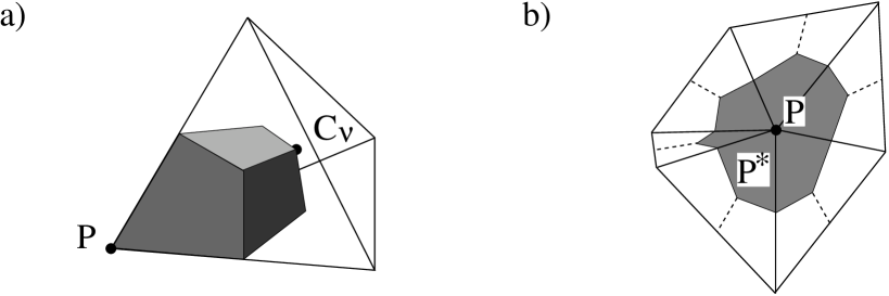
Figure 1: Panel a) shows the corner cell $a_{P}$ associated with the vertex $P$ of a 3-simplex. Notice that the intersection of $a_{P}$ with any of the triangular faces incident on $P$ is itself the two dimensional corner cell of $P$ in the triangular face, and that the six corners of $a_{P}$ are located at the centers of the simplices incident on $P$, defining, topologically, a cube.

Panel b) shows the cell $P^{*}$ dual to the vertex $P$ in a two dimensional simplicial complex. The boundaries of other dual cells are indicated by dashed lines. The cells and subcells of this realization of the dual complex generally are not flat where they meet a boundary between simplices.

In the definition of the simplicial model a central role will be played by the $2$-cells $s(\sigma\nu)$ of the derived complex which are attached to the centers of the 4-simplices. Each is associated with a 4-simplex $\nu$ and a 2-simplex $\sigma$ of $\nu$, and is a plane quadrilateral formed by the centers of $\nu$, $\sigma$, and the two 3-simplices $\tau_{1}$ and $\tau_{2}$ of $\nu$ that share $\sigma$. $s(\sigma\nu)$ can also be thought of as the restriction to $\nu$ of the cell $\sigma^{*}$ of the dual complex dual to $\sigma$. See Fig. 2.

$s(\sigma\nu)$ will be called a “wedge” and will often be denoted by just $s$ or $\sigma\nu$. 4-simplices will be denoted by $\nu$, with some additional subscripts or markings to distinguish different 4-simplices. 3-simplices will similarly be denoted by $\tau$, and 2-simplices by $\sigma$. 0-simplices, i.e. vertices, will be denoted by latin capitals $P,Q,R,...$. Finally, $\mu<\rho$ signifies that $\mu$ is a subcell or subsimplex of $\rho$ which may be a simplex, a cell of the derived complex, a cell of the dual complex, or a complex.

The 4-simplices will be given a uniform orientation throughout $\Delta$, and the orientation of each wedge $s(\sigma\nu)$ will be determined by the orientations of $\sigma$ and $\nu$ through the requirement that a positively oriented basis on $\sigma$ concatenated with a positively oriented basis on $s$ forms a positively oriented basis on $\nu$.

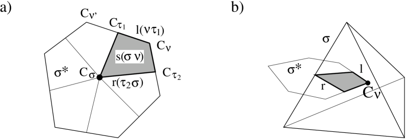
Figure 2: Panel a) illustrates the definitions of $s(\sigma\nu)$ and the edges $l(\nu\tau)$ and $r(\tau\sigma)$. In the middle lies the center of a 2-simplex $\sigma$. The corners are the centers of all the 4-simplices $\nu,\nu^{\prime},...$ that share $\sigma$. The curve $C_{\nu}C_{\tau_{1}}C_{\nu^{\prime}}$ connecting $C_{\nu}$ and $C_{\nu^{\prime}}$ is the edge $\tau_{1}^{*}$ in $\Delta^{*}$ which is dual to $\tau_{1}$. Similarly $\cup_{\nu}s(\sigma\nu)$ is the 2-cell $\sigma^{*}<\Delta^{*}$ dual to $\sigma$. One may think of $s(\sigma\nu)$ as the wedge of $\sigma^{*}$ in $\nu$: $s(\sigma\nu)=\sigma^{*}\cap\nu$. Likewise, $l(\nu\tau)=\tau^{*}\cap\nu$ and the radial edge $r(\tau\sigma)=\sigma^{*}\cap\tau$.

Panel b) shows the analogous structure in a 3-dimensional complex with a 3-simplex playing the role of $\nu$, 2-simplices as $\tau_{1}$ and $\tau_{2}$, and a 1-simplex as $\sigma$.

In the left-handed simplicial model of GR presented here one associates to each wedge $s(\sigma\nu)$ an $SU(2)$ spin 1 vector $e_{s\,i}$, which will more or less play the role of Plebanski’s $\Sigma_{i}$ field. The role of $A$ is played by $SU(2)$ parallel propagators along the edges of the $s(\sigma\nu)$. Specifically, there is an $h_{l}\in SU(2)$ for each edge $l(\nu\tau)$ from the center of 4-simplex $\nu$ to that of 3-simplex $\tau<\nu$, and there is a $k_{r}\in SU(2)$ for each edge $r(\tau\sigma)$ from the center of 3-simplex $\tau$ to that of 2-simplex $\sigma<\tau$.

Finally, a spin 2 $SU(2)$ tensor $\varphi_{\nu}$ (represented by a symmetric, traceless matrix, $\varphi^{ij}_{\nu}$) is associated with each 4-simplex. $\varphi^{ij}_{\nu}$ plays the role of $\phi^{ij}$.

The action for the model is

$$I_{\Delta}=\sum_{\nu<\Delta}[\sum_{s<\nu}e_{s\,i}\theta^{i}_{s}-\frac{1}{60}\varphi^{ij}_{\nu}\sum_{s,\bar{s}<\nu}e_{s\,i}e_{\bar{s}\,j}sgn(s,\bar{s})].$$ (3)

$\theta^{i}_{s}$ is a measure of the curvature on $s$. It is a function of the $SU(2)$ parallel propagators via

$$\theta^{i}_{s}=tr[J^{i}g_{\partial s}],$$ (4)

where $g_{\partial s}$ the holonomy around $\partial s$, and the $J_{i}$ are $1/2$ the Pauli sigma matrices $g_{\partial s}$ and $\theta_{s}$ may be written in terms of a rotation vector $\rho^{i}$ as

$$g_{\partial s} = e^{i\rho\cdot J}=\cos\frac{|\rho|}{2}{\bf 1}+2i\sin\frac{|\rho|}{2}\hat{\rho}\cdot J$$ (6)

$$\theta_{s} = 2\sin\frac{|\rho|}{2}\hat{\rho}$$ (7)

($\hat{\rho}=\rho/|\rho|$). The rotation vector is essentially the curvature on the wedge $s$, and, when the holonomy is close to one, i.e. the curvature is small, $\theta_{s}$ approximates the rotation vector.

$sgn(s,\bar{s})\equiv sgn(\sigma,\bar{\sigma})$ is essentially the sign of the oriented 4-volume spanned by the 2-simplices $\sigma$ and $\bar{\sigma}$ associated with $s$ and $\bar{s}$: If $\sigma$ and $\bar{\sigma}$ share only one vertex (the minimum number when both belong to the same 4-simplex), then the orientations of $\sigma$ and $\bar{\sigma}$ define an orientation for $\nu$, namely the orientation of the basis produced by concatenating positively oriented bases of $\sigma$ and $\bar{\sigma}$. If this orientation matches that already chosen for $\nu$ then $sgn(s,\bar{s})=1$. If it is the opposite $sgn(s,\bar{s})=-1$. If $\sigma$ and $\bar{\sigma}$ share 2 or 3 vertices they lie in the same 3-plane and span no 4-volume. In this case $sgn(s,\bar{s})=0$.

A nice, very explicit, formula can be given for the sum in the second term (3). If the vertices of the 4-simplex are numbered 1, 2, 3, 4, 5, so that 12, 13, 14, 15 form a positively oriented basis then

$$\sum_{s,\bar{s}<\nu}e_{s\,i}e_{\bar{s}\,j}sgn(s,\bar{s})=\frac{1}{4}\sum_{P,Q,R,S,T\in\{1,2,3,4,5\}}e_{PQR\,i}e_{PST\,j}\epsilon^{PQRST},$$ (8)

where $e_{PQR}=e_{s(PQR,\nu)}$, and $PQR$ indicates the 2-simplex with positively ordered vertices $P$, $Q$, $R$.

3 Field equations and boundary terms

Extremization of (3) with respect to $h_{l(\nu,\tau)}$ is most easily carried out by parametrizing variations of $h_{l}$ via $h_{l}+\delta h_{l}=h_{l}exp[i\alpha_{l}\cdot J]$. Then

$$itr[h_{l}J_{i}\frac{\partial I_{\Delta}}{\partial h_{l}}]=\frac{\partial I_{\Delta}}{\partial\alpha_{l}^{i}}|_{\alpha_{l}=0}.$$ (9)

On the other hand $l(\nu,\tau)\subset\partial s(\sigma,\nu)$ when $\sigma<\tau$, so such a variation of $h_{l}$ induces

$$g_{\partial\sigma\nu}\rightarrow g_{\partial\sigma\nu}e^{i\alpha_{l}\cdot J}.$$ (10)

(Here each $\sigma<\tau$ has been oriented to match $\partial\tau$ and $\tau$ to match $\partial\nu$, with the effect that $l$ is positively oriented in $\partial s(\sigma,\nu)$). Thus

$$\delta\theta^{i}=\alpha_{l}^{j}2tr[J_{j}J^{i}g_{\partial s}]$$ (11)

and

$$\delta I_{\Delta}=ag_{l}\cdot\sum_{\sigma<\tau}w_{\sigma\nu},$$ (12)

with

$$w_{s\,j}=2tr[J_{j}J^{i}g_{\partial s}]e_{s\,i}=\cos\frac{|\rho|}{2}e_{s\,j}+2\sin\frac{|\rho|}{2}[\hat{\rho}\times e_{s}]_{j}$$ (13)

Extremization with respect to $h_{l(\nu\tau)}$ thus requires

$$0=itr[h_{l}J_{i}\frac{\partial I_{\Delta}}{\partial h_{l}}]=\sum_{\sigma<\tau}w_{\sigma\nu\,i}. *14$$ ()

(The field equations are numbered with $*$s). Similarly, extremization with respect to $k_{r(\tau\sigma)}$ requires

$$u_{\sigma\nu_{1}}=u_{\sigma\nu_{2}} *15$$ ()

where $\nu_{1}$ and $\nu_{2}$ are the two 4-simplices sharing $\tau$, and

$$u_{\sigma\nu_{1}\,i}=U^{(1)}[k_{r(\tau\sigma)}h_{l(\nu_{1}\tau)}]_{i}{}^{j}w_{\sigma\nu_{1}\,j}.$$ (16)

($U^{(1)}(g)$ is the spin 1 representation of $g\in SU(2)$). In general $u_{\sigma\nu}$ is $w_{\sigma\nu}$ parallel transported from $C_{\nu}$ along the boundary $\partial s(\sigma\nu)$ in a positive sense to $C_{\sigma}$. (See Fig. 3). $u_{s}$ is thus, like $w_{s}$, $e$ multiplied by a factor which goes to one as the group elements $h_{l}$ and $k_{r}$ approach ${\bf 1}$. Note that ($*15$) implies that all $u_{\sigma\nu}$ for a given 2-simplex $\sigma$ have a common value $u_{\sigma}$.

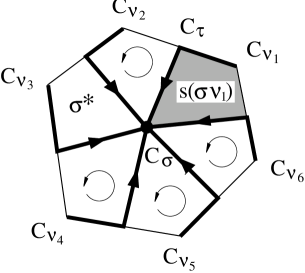
Figure 3: The dual 2-cell $\sigma^{*}<\Delta^{*}$ is shown with its uniform orientation indicated by an arrow circling in a positive sense. The routes by which the $w_{\sigma\nu_{n}}$ are parallel transported from $C_{\nu_{n}}$ to $C_{\sigma}$ to form the $u_{\sigma\nu_{n}}$ are indicated by bold lines.

Extremization with respect to $\varphi_{\nu}^{ij}$ yields

$$\frac{\partial I_{\Delta}}{\partial\varphi^{ij}_{\nu}}=\frac{1}{60}\sum_{s,\bar{s}<\nu}e_{s\,i}e_{\bar{s}\,j}sgn(s,\bar{s})\propto\delta_{ij} *17$$ ()

(since $\varphi^{ij}_{\nu}$ is traceless).

Finally, extremization with respect to $\bar{e}_{s}$ implies

$$\frac{\partial I_{\Delta}}{\partial e_{s\,i}}=\theta^{i}_{s}-\frac{1}{30}\varphi^{ij}_{\nu}\sum_{\bar{s}<\nu}e_{\bar{s}\,j}sgn(s,\bar{s})=0. *18$$ ()

What about boundary terms? Suppose the simplicial complex has a boundary $\partial\Delta$ which doesn’t cut through any 4-simplex, so it is itself a 3 dimensional simplicial complex. No boundary term needs to be added to the action (3) if the connection is held fixed at that boundary, that is to say, if the group elements $k_{r}$ on the edges $r(\tau,\sigma)$ in the boundary are held fixed. ($r(\tau\sigma)$ in the boundary is the intersection of $\tau<\partial\Delta$ and the 1-cell in the dual, $[\partial\Delta]^{*}$, of the the boundary which is dual to $\sigma$).

Another natural field to hold fixed is $u_{\sigma}$ for $\sigma<\partial\Delta$ (since it lives on the boundary, unlike $e_{\sigma\nu}$ and $w_{\sigma\nu}$ which live in the internal space at $C_{\nu}$, and thus always off the boundary). This corresponds more closely to what is usually done in Regge calculus [Reg61], that is, holding the lengths of the edges fixed on the boundary, because $e_{\sigma\nu}$, and therefore $u_{\sigma}$, is essentially the metrical field variable in the present simplicial model. (See Appendix A for more on the relation of $e_{\sigma\nu}$ and $u_{\sigma}$ to metric geometry). In this case the action must be modified: In the modified action the $\theta_{s}$ for $s$ abutting the boundary are evaluated with $k_{r}$ replaced by ${\bf 1}$ $\forall r<\partial\Delta$ (but the definition of $u_{\sigma}$, (16), is unchanged).

4 The continuum limit

The form of the action (3) is clearly analogous to that of the Plebanski action (1). Moreover, Plebanski’s field equations

$$\frac{\delta I_{P}}{\delta\phi^{ij}} = \frac{1}{2}\Sigma_{i}\wedge\Sigma_{j}\propto\delta_{ij}$$ (19)

$$\frac{\delta I_{P}}{\delta A^{i}} = D\wedge\Sigma_{i}=0$$ (20)

$$\frac{\delta I_{P}}{\delta\Sigma_{i}} = F^{i}-\phi^{ij}\Sigma_{j}=0$$ (21)

resemble simplicial field equations ($*17$), ($*14$), and ($*18$) respectively. We shall see that in the continuum limit these resemblances become exact. (The simplicial field equation ($*15$) has no continuum analog, it is an identity in the continuum limit I will define).

In order to take the continuum limit of the simplicial theory I define below a map $\Omega_{\Delta}$ of continuum fields on a compact spacetime manifold $M$ into simplicial fields on a simplicial decomposition $\Delta$ of $M$, which allows us to represent continuum field histories by simplicial ones, and a class of sequences $\{\Delta_{n}\}_{n=0}^{\infty}$ of simplicial decompositions of spacetime which become infinitely fine everywhere in a nice way as $n\rightarrow\infty$. Any continuum field history $(A,\Sigma,\phi)$ then defines a sequence of increasingly faithful images $\Omega_{n}(A,\Sigma,\phi)=(h,k,e,\varphi)_{n}$ on the complexes $\Delta_{n}$, and corresponding evaluations $I_{n}(A,\Sigma,\phi)$ of the simplicial action.

I will confine myself to showing that a continuum limit of the simplicial model reproduces the Plebanski theory for continous $\phi$ and continously differentiable $A$ and $\Sigma$. On such fields the Plebanski lagrangian, and the functional derivatives of the action, are continous. Unless otherwise stated $A$, $\Sigma$, and $\phi$ will be assumed to satisfy these continuity/differentiability requirements from now on.

I will begin by showing that the evaluations $I_{n}$ of the simplicial action converge to the Plebanski action in the limit of infinitely fine simplicial decompositions: $I_{n}(A,\Sigma,\phi)\rightarrow I_{P}(A,\Sigma,\phi)$ as $n\rightarrow\infty$. Unless $I_{n}(A,\Sigma,\phi)$ has a more and more oscillatory dependence on $A$, $\Sigma$, and $\phi$ as $n\rightarrow\infty$ it follows that the variations of the simplicial action due to variations $\delta A$, $\delta\Sigma$, and $\delta\phi$ of the continuum fields converge to the corresponding variantions of the Plebanski action. That this is in fact the case will be verified directly. The Plebanski theory is thus the continuum limit of the simplicial theory in the weak sense that the solutions of the Plebanski theory are the continuum field configurations that extremize the simplicial action with respect to variations of the continuum fields. In terms of field equations, or more precisely in terms of the variational derivatives of the actions - which will be called the “Euler-Lagrange functions” (E-L functions), one can say that $A$, $\Sigma$, and $\phi$ solve the Plebanski field equations iff the simplicial E-L functions evaluated on their image $(h,k,e,\varphi)_{n}=\Omega_{n}(A,\Sigma,\phi)$ integrated against the image $(\delta h,\delta k,\delta e,\delta\varphi)_{n}$ of the variations $\delta A$, $\delta\Sigma$, and $\delta\phi$ vanish as $n\rightarrow\infty$.

In fact a stronger result will be proved: the E-L functions vanish more rapidly as $\nu\rightarrow\infty$ on solutions to the Plebanski equations than on non-solutions. The simplicial E-L functions ($*17$), ($*14$), and ($*18$) on the image of a continuum field configuration turn out to be simply the integrals of the Plebanski E-L $d$-forms (19), (20), and (21) over suitable $d$-cells in each 4-simplex, modulo corrections of higher order in the radius $r_{\nu}$ of the 4-simplex (where the radius is determined by an arbitrarily chosen positive definite background metric on spacetime). As a consequence the simplicial E-L functions of the image of any continuum field configuration, whether solution or not, will vanish as $n\rightarrow\infty$, simply because the cells over which the corresponding Plebanski E-L forms are integrated get smaller as the complex is refined. Specifically, the leading term in the E-L function ($*14$) vanishes as $r_{\nu}^{3}$, that in ($*17$) as $r_{\nu}^{4}$, and that in ($*18$) as $r_{\nu}^{2}$. The integrals in each 4-simplex are sufficient to detect any non-zero components of the E-L forms when the simplex is sufficiently small. It therefore also follows that a continuum field configuration is a solution of the Plebanski field equations iff all the E-L functions vanish more rapidly than the non-solution rate as $n\rightarrow\infty$.

That the simplicial field equations converge to those of the Plebanski theory in this stronger sense is significant. M. Miller [Mil95] and Brewin [Bre95] have found that the analogous result does not hold for the Regge model [Reg61]! One can define a natural simplicial image of a metric on a spacetime $M$ by covering $M$ with a simplicial complex with geodesic edges and taking as the length of each edge its metric length in $M$. What Miller and Brewin found is that on the images of most solutions to Einstein’s equations (including the Kerr solution [Mil95]) the Regge E-L functions do not vanish any more rapidly, as the complex is refined, than on non-solutions. On the other hand, Miller, and Brewin, also showed that certain linear combinations of the Regge E-L functions do vanish more rapidly than the non-solution rate. These combinations are essentially $\partial I_{Regge}/\partial g_{\mu\nu}$ in a cell built out of several adjacent simplices. Their rapid vanishing guarantees that GR is the continuum limit of the Regge theory in the weak sense that solutions (and only solutions) to GR extremize the Regge action with respect to variations of the continuum metric in the limit of an infinitely fine simplicial complex.

What is going on? As the simplicial complex is refined, and becomes much finer than the scale on which a given $\delta g_{\mu\nu}$ varies, the corresponding variations of the edge lengths, $\delta l$, approach those due to a constant $\delta g_{\mu\nu}$, which are highly correlated in spacetime. Thus extremization (modulo error terms which vanish as the complex is refined) with respect to continuum metric modes is a much weaker requirement than extremization with respect to all edge length. It leaves many modes of the edge lengths free, because it allows many non-zero distributions of values of the E-L functions over the complex. On the other hand, the fineness of the simplicial complex also restricts the possible modes of the edge lengths in images of continuum metrics. On a suffiently fine complex the metric will be nearly constant, and the distribution of edge lengths, and similarly values of the E-L functions, will be severely restricted simply by virtue of the fact that the edge lengths are the image of a continuum metric. The question is then whether these restrictions, together with the field equations that come from extremizing with respect to the continuum metric, are enough to imply that all the simplicial E-L functions vanish (faster than the non-solution rate as the complex is refined). In the Regge model the restrictions are not quite enough. In the simplicial model presented here the analogous mechanism does work.

The result of Miller and Brewin seems a serious problem for path integral quantizations based on the Regge model. A path integral over the edge lengths will not have stationary phase trajectories corresponding to the full set of solutions of Einsteins equations, and thus will not provide a quantization of general relativity. One would have to integrate over some restricted set of simplicial spacetimes, but to my knowledge no such restricted path integral has been defined. (How these considerations bear on dynamical triangulation path integrals [Wei82] based on the Regge action is unclear to me). In contrast, a path integral over the fundamental variables of the simplicial model presented here is, at least on this count, a viable model of quantum general relativity.

In the present work it is shown that the smooth solutions of the simplicial theory, i.e. solutions which are images of $A$, $\Sigma$, $\phi$ on complexes much finer than the scale on which these fields vary, are in fact the solutions of Plebansk’s field equations. What is not shown is that smooth boundary or initial data cannot lead to solutions which are highly crumpled, in addition to the smooth solutions, or that solutions that are crumpled on the simplicial scale approximate continuum solutions on larger scales.

Now to the details.

Definition 1: The map $\Omega_{\Delta}:(A,\Sigma,\phi)\mapsto(h,k,e,\varphi)$ of continuum fields on $M$ to simplicial fields on the simplicial decomposition $\Delta$ of $M$ is defined by

$$h_{l} = {\cal P}e^{i\int_{l}A\cdot J}$$ (22)

$$k_{r} = {\cal P}e^{i\int_{r}A\cdot J}$$ (23)

$$u_{\sigma\nu\,i} = \int_{\sigma}v(C_{\sigma},x)_{i}{}^{j}\Sigma_{j}(x)$$ (24)

$$\varphi^{ij}_{\nu} = \phi^{ij}(C_{\nu})$$ (25)

with $e_{\sigma\nu}$ defined from $u_{\sigma}$ via (16) and (13),

${\cal P}$ denotes path ordering, and $v(C_{\sigma},x)=U^{(1)}({\cal P}e^{i\int_{C_{\sigma}}^{x}A\cdot J})$ is the parallel propagator of spin 1 $SU(2)$ vectors along a straight line from $x$ to $C_{\sigma}$ (according to the affine structure of $\sigma$).

This definition of $\Omega_{\Delta}$ is not the only one possible. Other maps also lead to equivalence of the continuum limit of the simplicial theory and the Plebanski theory. For instance maps such that $h$, $k$, $e$, $\varphi$ converge to those of Definition 1 as the simplicial complex is refined are viable alternatives. However the $\Omega_{\Delta}$ chosen here seems to lead to the cleanest proofs.

Before considering the simplicial complexes to be used note that we will be concerned with compact spacetimes or compact pieces of spacetimes, which always admit finite simplicial decompositions

As the sequence of progressively finer simplicial decompositions I will use uniformly refining sequences, which are defined as follows.

Definition 2: $\{\Delta_{n}\}_{n=0}^{\infty}$ is a uniformly refining sequence of simplicial decompositions of a compact manifold $M$ if

1) $\Delta_{0}$ is a finite simplicial decomposition of $M$,

2) $\Delta_{n+1}$ is a finite refinement of $\Delta_{n}$,

and, in a fixed positive definite metric $g_{0}$ which is constant on each $\nu<\Delta_{0}$ (in linear coordinates on $\nu$),

3) $r_{n}$, the maximum of the radii $r_{\nu}$ of the 4-simplices $\nu<\Delta_{n}$ approaches zero as $n\rightarrow\infty$, and

4) $r_{\nu}^{4}$ divided by the 4-volume of $\nu$ is uniformly bounded for all 4-simplices $\nu<\Delta_{n}$ as $n\rightarrow\infty$.

In Appendix B it is proven that conditions 3) and 4) are independent of the particular metric chosen.

The following lemma, also proven in Appendix B, will be useful

Lemma 1: If $h$ is a continous $d$-form on a compact manifold $M$, $\{\Delta_{n}\}_{n=0}^{\infty}$ is a uniformly refining sequence of simplicial decompositions of $M$, and $g_{0}$ is a positive definite metric constant on each $\nu<\Delta_{0}$, then $\forall\epsilon>0$ $N$ can be chosen sufficiently large so that for any $d$-subcell $c$ of a 4-simplex $\nu<\Delta_{N}$

$$|\int_{c}h-\int_{c}h_{C_{\nu}}|<\epsilon r_{\nu}^{d},$$ (26)

where $h_{C_{\nu}}$ is the constant $d$-form (in linear coordinates on $\nu$) which agrees with $h$ at $C_{\nu}$, and $r_{\nu}$ is the $g_{0}$ radius of $\nu$.

Lemma 1 can be conveniently restated in terms of the characteristic tensor of $c$, which can be defined in linear coordinates $x^{\alpha}$ on $\nu$ by

$$t_{c}^{\alpha_{1}...\alpha_{d}}=\int_{c}dx^{\alpha_{1}}\wedge...\wedge dx^{\alpha_{d}}.$$ (27)

$t_{c}$ might be called the coordinate volume tensor of $c$, it is the $d$-dimensional generalization of the coordinate length vector of an edge and the coordinate area bivector of a 2-cell. When $c$ is a d-simplex with vertices $P_{1},...,P_{d+1}$ $t_{c}^{\alpha_{1}...\alpha_{d}}=(P_{1}P_{2})^{[\alpha_{1}}...(P_{1}P_{d+1})^{\alpha_{d}]}$. Using $t_{c}$ equation (26) in Lemma 1 can be written as

$$\int_{c}h=\int h(C_{\nu})_{\alpha_{1}...\alpha_{2}}t_{c}^{\alpha_{1}...\alpha_{2}}+O(\epsilon r_{\nu}^{d}),$$ (28)

where $O(\epsilon r_{\nu}^{d})$ denotes a quantity $Q_{c}$ that vanishes faster than $r_{\nu}^{d}$ as $n\rightarrow\infty$, that is, $max\{Q_{c}/r_{\nu}^{d}|c<\nu<\Delta_{n}\}\rightarrow 0$ as $n\rightarrow\infty$.

Now we are ready to prove that the simplicial action (3) converges to the Plebanski action in the continuum limit.

Theorem 1: If $\{\Delta_{n}\}_{n=0}^{\infty}$ is a uniformly refining sequence of simplicial decompositions of a compact, orientable 4-manifold, $M$; $A$, $\Sigma$, $\phi$ are Plebanski fields on $M$ with $\Sigma$ and $\phi$ continous and $A$ continously differentiable; and $I_{n}(A,\Sigma,\phi)$ is the evaluation of the simplicial action (3) on the simplicial fields $(h,k,e,\varphi)_{n}=\Omega_{\Delta_{n}}(A,\Sigma,\phi)$ defined on $\Delta_{n}$ by (22) - (25), then

$$lim_{n\rightarrow\infty}I_{n}(A,\Sigma,\phi)=I_{P}(A,\Sigma,\phi).$$ (29)

Proof: Choose a positive definite metric $g_{0}$ which is constant on each $\nu<\Delta_{0}$. By several applications of Lemma 1 one shows that $\forall\epsilon>0$ $N$ may be chosen large enough so that

$$|\theta_{\sigma\nu}^{i} - F(C_{\nu})^{i}_{\alpha\beta}t_{s(\sigma\nu)}^{\alpha\beta}|<\epsilon r_{\nu}^{2}$$ (30)

$$|e_{\sigma\nu\,i} - \Sigma(C_{\nu})_{\alpha\beta\,i}t_{\sigma}^{\alpha\beta}|<\epsilon r_{\nu}^{2}$$ (31)

$\forall\sigma<\nu<\Delta_{n}$. Thus

$$I_{N} = \sum_{\nu<\Delta_{N}}[\Sigma_{i\,\alpha\beta}F^{i}_{\gamma\delta}|_{C_{\nu}}\sum_{\sigma<\nu}t_{\sigma}^{\alpha\beta}t_{s(\sigma,\nu)}^{\gamma\delta}$$ (32)

$$\ \ \ \ -\frac{1}{60}\phi^{ij}\Sigma_{i\,\alpha\beta}\Sigma_{j\,\gamma\delta}|_{C_{\nu}}\sum_{\sigma,\bar{\sigma}<\nu}t_{\sigma}^{\alpha\beta}t_{\bar{\sigma}}^{\gamma\delta}sgn(\sigma,\bar{\sigma})+\Delta I_{N\nu}],$$

where the error term $\Delta I_{N\nu}$ is bounded by

$$|\Delta I_{N\nu}|<\epsilon r_{\nu}^{4}[10||F||+(10+\frac{1}{2}||\phi||)(||\Sigma||+\epsilon)]|_{C_{\nu}}$$ (33)

(Here the norm $||T||$ of a tensor $T^{i_{1}...i_{m}}_{\alpha_{1}...\\ ag_{n}}$ is $||T||=(T^{i_{1}...i_{m}}_{\alpha_{1}...\\ ag_{n}}T^{j_{1}...j_{m}}_{\beta_{1}...\\ bg_{n}}\delta_{i_{1}j_{1}}...g_{0}^{\alpha_{1}\beta_{1}}...)^{\frac{1}{2}}$). Since $F$, $\Sigma$, and $\phi$ are continous on the compact manifold $M$ they are bounded, so $|\Delta I_{N\nu}|<\epsilon r_{\nu}^{4}\kappa$ with $\kappa$ a finite constant.

The ratio of $r_{\nu}^{4}$ to the 4-volume $V_{\nu}$ of $\nu$ is uniformly bounded. Let this bound be $R$ then $r_{\nu}^{4}<RV_{\nu}$ implying that $|\Delta I_{N\nu}|<\epsilon\kappa RV_{\nu}$. Therefore the sum of the errors is bounded by

$$|\sum_{\nu<\Delta_{N}}\Delta I_{N\nu}|<\epsilon\kappa RV_{M},$$ (34)

where $V_{M}$ is the $g_{0}$ volume of $M$, a finite number.

Straightforward calculations show

$$\sum_{\sigma,\bar{\sigma}<\nu}t_{\sigma}^{\alpha\beta}t_{\bar{\sigma}}^{\gamma\delta}sgn(\sigma,\bar{\sigma}) = 30t_{\nu}^{\alpha\beta\gamma\delta}$$ (35)

$$\sum_{\sigma<\nu}t_{\sigma}^{\alpha\beta}t_{s(\sigma\nu)}^{\gamma\delta} = t_{\nu}^{\alpha\beta\gamma\delta}.$$ (36)

Thus, putting everything together, we get

$$I_{N} = [\sum_{\nu}(\Sigma_{i\,\alpha\beta}F^{i}_{\gamma\delta}-\frac{1}{2}\phi^{ij}\Sigma_{i\,\alpha\beta}\Sigma{j\,\gamma\delta})|_{C_{\nu}}t_{\nu}^{\alpha\beta\gamma\delta}]+\Delta I_{N}$$ (37)

$$\stackrel{{\scriptstyle\longrightarrow}}{{\scriptstyle{N\rightarrow\infty}}} \int_{M}\Sigma_{i}\wedge F^{i}-\frac{1}{2}\phi^{ij}\Sigma_{i}\wedge\Sigma_{j}=I_{P}(A,\Sigma,\phi).$$ (38)

 

To prove the equivalence of the continuum limit of the simplicial model with Plebanski’s theory at the level of field equations I show that the Euler-Lagrange (E-L) functions, i.e. the variational derivatives of the action with respect to the fields, are just the integrals of the Euler-Lagrange $d$-forms of the Plebanski theory over certain $d$-cells, modulo corrections which become negligible as the simplicial complex is refined. Then, if a “continuum limit solution” of the simplicial model is defined to be a continuum field configuration, $(A,\Sigma,\phi)$ such that its simplicial images $\Omega_{n}(A,\Sigma,\phi)=(h,k,e,\varphi)_{n}$ have E-L functions that vanish faster than the volumes of the corresponding $d$-cells as $n\rightarrow\infty$, the continuum limit solutions are precisely the solutions to the Plebanski field equations.

The precise statement I will prove is

Theorem 2: Under the hypothesies of Theorem 1 and the additional condition that $\Sigma$ is continously differentiable the following hold for any simplicial field history corresponding to a continuum field history via (22) - (25):

1) The simplicial field equation ($*15$) $tr[J_{i}k_{r}\frac{\partial I_{n}}{\partial k_{r}}]=0$ holds identically for all $n$.

2) $\forall\nu<\Delta_{n},\ \ s,l<\nu$

$$\frac{\partial I_{n}}{\partial\varphi^{ij}_{\nu}} = \int_{\nu}\frac{\delta I_{P}}{\delta\phi^{ij}}+O(\epsilon r_{\nu}^{4})$$ (39)

$$\frac{\partial I_{n}}{\partial e_{s\,i}} = \int_{s}\frac{\delta I_{P}}{\delta\Sigma_{i}}+O(\epsilon r_{\nu}^{2})$$ (40)

$$itr[h_{l}J_{i}\frac{\partial I_{n}}{\partial h_{l}}] = \int_{\tau}\frac{\delta I_{P}}{\delta A^{i}}+O(\epsilon r_{\nu}^{3})$$ (41)

where $\tau$ is the 3-simplex in $\nu$ dual to $l$, and in the integrals the integrands are parallel transported to $C_{\nu}$ along straight lines.

3) The Plebanski field equations are fully represented by the simplicial field equations in the sense that if the Plebanski E-L forms are not almost everywhere zero, then on a sufficiently fine simplicial complex the simplicial E-L functions will not all vanish.

Proof: 1) follows immediately from the definition (24) of $u_{\sigma\nu}(A,\Sigma)$. (39) and (41) from the corresponding Plebanski field equations (19) and (20) and

$$\frac{\partial I_{n}}{\partial\phi^{ij}_{\nu}} = \frac{1}{60}\sum_{\sigma,\bar{\sigma}<\nu}e_{\sigma\nu\,i}e_{\bar{\sigma}\nu\,j}sgn(\sigma,\bar{\sigma})$$ (42)

$$= (\Sigma_{i\,\alpha\beta}\Sigma_{j\,\gamma\delta})|_{C_{\nu}}\frac{1}{60}\sum_{\sigma,\bar{\sigma}<\nu}t_{\sigma}^{\alpha\beta}t_{\bar{\sigma}}^{\gamma\delta}sgn(\sigma,\bar{\sigma})+O(\epsilon r_{\nu}^{4})$$ (43)

$$= \frac{1}{2}(\Sigma_{i}\wedge\Sigma_{j})|_{C_{\nu}\ \alpha\beta\gamma\delta}t_{\nu}^{\alpha\beta\gamma\delta}+O(\epsilon r_{\nu}^{4})$$ (44)

$$itr[h_{l}J_{i}\frac{\partial I_{n}}{\partial h_{l}}] = \sum_{\sigma<\tau}w_{\sigma\nu\,i}=h_{l\,i}^{-1}{}^{j}\sum_{\sigma<\tau}k_{r(\tau\sigma\,j}^{-1}{}^{k}u_{\sigma\,k}$$ (45)

$$= (D\wedge\Sigma_{i})|_{C_{\nu}\ \alpha\beta\gamma}t_{\tau}^{\alpha\beta\gamma}+O(\epsilon r_{\nu}^{3}).$$ (46)

Similarly (40) follows from (21) and the identity $\sum_{\bar{\sigma}<\nu}t_{\bar{\sigma}}^{\alpha,\beta}sgn(\sigma,\bar{\sigma})=30t_{s(\sigma,\nu)}^{\alpha\beta}$ via

$$\frac{\partial I_{n}}{\partial e_{s\,i}} = \theta^{i}_{\sigma\nu}-\frac{1}{30}\varphi^{ij}_{\nu}\sum_{\bar{\sigma}<\nu}e_{\bar{\sigma}\nu\,j}sgn(\sigma,\bar{\sigma})$$ (47)

$$= (F^{i}-\phi^{ij}\Sigma_{j})|_{C_{\nu}\ \alpha\beta}t_{s(\sigma\nu)}^{\alpha\beta}+O(\epsilon r_{\nu}^{2}).$$ (48)

3) follows as a corrollary of 2). Condition 4) in Definition 2, which defines $\Delta_{n}$, prevents the 4-simplices from having zero volume, and therefore ensures that in each such 4-simplex $\nu<\Delta_{n}$ the $t_{s}$, $t_{\tau}$, $t_{\nu}$ span the spaces of 2, 3, and 4 index antisymmetric tensors at $C_{\nu}$.  

Using (9) and the fact that under variations of $A$, $\Sigma$, $\phi$ the variations of the corresponding simplicial fields $h$, $e$, $\varphi$ are given by

$$\delta\varphi^{ij}_{\nu} = \delta\phi^{ij}(C_{\nu})$$ (49)

$$\delta e_{\sigma\nu\,i} = \int_{\sigma}\delta\Sigma_{i}+O(\epsilon r_{\nu}^{2})$$ (50)

$$\delta\alpha^{i}_{l} = \int_{l}\delta A^{i}+O(\epsilon r_{\nu})$$ (51)

(where the integrands are parallel transported to $C_{\nu}$ along straight lines). one finds that

Corollary: The hypothesies of Theorem 1 and $\Sigma$ continously differentiable imply that, under variations of $A$, $\Sigma$, and $\phi$

$$\lim_{n\rightarrow\infty}\delta I_{n}(A,\Sigma,\phi)=\delta I_{P}(A,\Sigma,\phi).$$ (52)

5 Comments

$\bullet$ A hypercubic lattice action for GR can be defined in complete analogy with the simplicial one. One defines the centers of $n$-cubes as the averages of their vertices, and the dual complex from these centers as in the simplicial context. In particular, the wedges $s$, and the edges $l$ and $r$ are defined by replacing $n$-simplices with $n$-cubes in their simplicial definitions. (See Fig. 4).

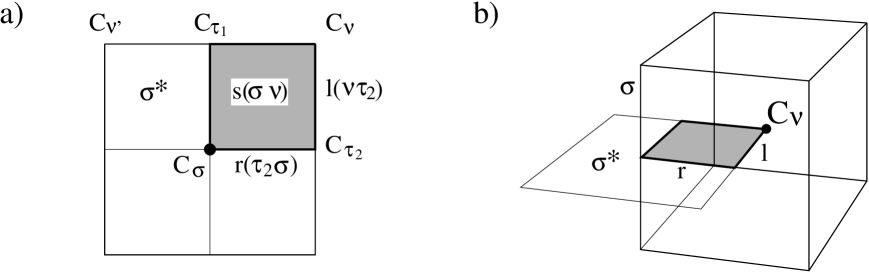
Figure 4: This is the analogue of Fig. 2 for a hypercubic lattice. Panel a) illustrates the definitions of $s(\sigma\nu)$ and the edges $l(\nu\tau)$ and $r(\tau\sigma)$. In the middle lies the center of a 2-cube $\sigma$. The corners are the centers of all the 4-cubes $\nu,\nu^{\prime},...$ that share $\sigma$. The curve $C_{\nu}C_{\tau_{1}}C_{\nu^{\prime}}$ connecting $C_{\nu}$ and $C_{\nu^{\prime}}$ is the edge $\tau_{1}^{*}$ in the lattice $\Box^{*}$ dual to $\Box$, which is dual to $\tau_{1}$. Similarly $\cup_{\nu}s(\sigma\nu)$ is the 2-cell $\sigma^{*}<\Box^{*}$ dual to $\sigma$.

Panel b) shows the analogous structure in a 3-dimensional cubic lattice with a 3-cube playing the role of $\nu$, 2-cubes as $\tau_{1}$ and $\tau_{2}$, and a 1-cube as $\sigma$.

The action of the hypercubic model is

$$I_{\Box}=\sum_{\nu<\Box}[\sum_{s<\nu}e_{s\,i}\theta^{i}_{s}-\frac{1}{8}\varphi^{ij}_{\nu}\sum_{s,\bar{s}<\nu}e_{s\,i}e_{\bar{s}\,j}\ sgn(s,\bar{s})],$$ (53)

where $\Box$ is the hypercubic lattice and $\nu$ labels 4-cubes. $sgn(s,\bar{s})=sgn(\sigma,\bar{\sigma})$ is the sign of the 4-volume spanned by the 2-cubes (squares) $\sigma$ and $\bar{\sigma}$ dual to $s$ and $\bar{s}$ respectively, provided $\sigma$ and $\bar{\sigma}$ share one vertex. Otherwise $sgn(s,\bar{s})=0$. In particular this means that it is zero when the 2-cubes share no vertices.

Plebanski theory is the continuum limit of the hypercubic theory (53) in the same sense as it is the continuum limit of the simplicial theory. (The proofs of section 4 go through with minor adjustments).

$\bullet$ Boström, M. Miller and Smolin [BMS94] found a hypercubic lattice action corresponding to the CDJ action [CDJ91] (which is closely related to that of Plebanski) by following the method of Regge [Reg61] and evaluating the continuum action on field configurations in which the curvature has support only on the 2-dimensional faces of a spacetime lattice. Unfortunately, the continuum action is not unambigously defined on such field configurations. Nevertheless, Boström et. al. present an action corresponding to a particular disambiguation of this expression. This action, written in terms of the discrete curvature variable of Boström et. al. is formally similar to that one obtains from (53) by eliminating $e_{s}$ using the field equations. However, their curvature is defined very differently from the curvature ($\theta_{s}$) used here, in terms of the fundamental fields, which in their case is a discrete connection $1$-form and in the present case is the set of parallel propagators.

$\bullet$ Several authors [ReS89], [Imm94], [Loll95], [Zap96] have proposed canonical lattice formulations of general relativity using lattice analogs of the Ashtekar variables. It would be very interesting to compare the present model with these canonical theories. This would require a canonical formulation of the present model, which has not yet been found. Perhaps an approach similar to that of [Kha95] would work.

$\bullet$ The simplicial theory presented here converges in the continuum limit to Plebanski’s theory, which is not equivalent to Ashtekar’s canonical theory when the spatial metric is degenerate. Thus one would expect a quantization of the present simplicial model to approximate a quantization of the constraints of [Rei95] rather than Ashtekar’s constraints.

Appendix A The simplicial field $e_{s}$ and metric geometry

On non-degenerate solutions Plebanski’s fields $A$, $\Sigma$, $\phi$ have metrical interpretations. Thus simplicial fields defined via (22) - (25) should also have a metrical interpretation. In fact, when $\Sigma_{i}$ satisfies the field equation (19) $\Sigma_{i}\wedge\Sigma_{j}\propto\delta_{ij}$, and the non-degeneracy requirement $\Sigma_{k}\wedge\Sigma^{k}\neq 0$, it defines a non-degenerate cotetrad $e^{I}{}_{\alpha}$ (unique up to $SO(3)_{L}$ transformations) and thus a non-degenerate metric

$$g_{\alpha\beta}=e^{I}{}_{\alpha}\delta_{IJ}e^{J}{}_{\beta}.$$ (54)

Furthermore, when $A$ obeys the field equation $D\wedge\Sigma_{i}=0$, the Plebanski action becomes the Einstein-Hilbert action of the metric (54), so this metric is the physical metric.

On solutions of (19) $\Sigma_{i}=2[e\wedge e]^{+\,0i}$, where

$$[e\wedge e]^{+\,IJ}=\frac{1}{2}e^{I}\wedge e^{J}+\frac{1}{4}\epsilon^{IJ}{}_{KL}e^{K}\wedge e^{L}$$ (55)

is the self-dual part of $e\wedge e$. Therefore, by (24), the simplicial variable $e_{\sigma\nu}$ is the self-dual part of the metric area bivector of $\sigma$ (modulo corrections that vanish faster than the area as the simplicial complex is refined):

$$e_{\sigma\nu\,i}=\int_{\sigma}\Sigma_{i}+O(\epsilon r_{\nu}^{2})=2a_{\sigma}^{+\,0i}+O(\epsilon r_{\nu}^{2}),$$ (56)

with $a_{\sigma}^{IJ}=e^{I}{}_{\alpha}e^{J}{}_{\beta}|_{C_{\nu}}t_{\sigma}^{\alpha\beta}$ the metric area bivector, equal to the coordinate area bivector in metric normal coordinates.

If normal coordinates $x^{I}$ are chosen so that $\sigma$ lies in a spatial hypersurface ($x^{0}=\mbox{\em constant}$) then $e_{\sigma\nu\,i}=\frac{1}{2}\epsilon^{i}{}_{jk}a_{\sigma}^{jk}$ - exactly the normal area vector of $\sigma$.

It would be nice to give a metric interpretation of $e_{\sigma\nu}$ also away from the continuum limit, to make possible a direct comparison of the present simplicial theory with Regge calculus [Reg61]. This is difficult since, unlike in Regge calculus, the simplices of the present model are not flat. The wedges, $s$, carry curvature, $\theta_{s}$, which does not generally vanish, even on solutions.

However, when the holonomies $g_{\partial s}$ are all ${\bf 1}$ the metric interpretation of the continuum limit extends to arbitrary simplicial complexes. The only non-degenerate solutions satisfying this requirement exactly are flat spacetimes, even though in continuum euclidean GR there are curved non-degenerate solutions with vanishing self-dual curvature. It seems that the discrete solutions approximating curved non-degenerate anti-self-dual solutions necessarily have some self-dual curvature. Nevertheless, it is interesting to see how the metric emerges even in flat solutions.

With $g_{\partial s}={\bf 1}$, $w_{s}=e_{s}$, so field equation ($*14$) requires

$$\sum_{\sigma<\tau}e_{\sigma\nu\,i}=0.$$ (57)

(57) imposes 12 independent linear constraints on the 30 $e_{\sigma\nu\,i}$, which imply just that there is a 2-form $\Sigma_{\nu\,i\,\alpha\beta}$ (18 components) such that

$$e_{\sigma\nu\,i}=\Sigma_{\nu\,i\,\alpha\beta}t_{\sigma}^{\alpha\beta}.$$ (58)

Field equation ($*17$) and the non-degeneracy condition

$$\sum_{\sigma,\bar{\sigma}<\nu}e_{\sigma\nu}\cdot e_{\bar{\sigma}\nu}sgn(\sigma,\bar{\sigma})\neq 0$$ (59)

are equivalent to $\Sigma_{\nu\,i}\wedge\Sigma_{\nu\,j}\propto\delta_{ij}$ with $\Sigma_{\nu\,k}\wedge\Sigma_{\nu}^{k}\neq 0$. As for the continuum $\Sigma$ fields this implies $\Sigma$ defines a non-degenerate metric, and that $e_{\sigma\nu}$ is the self-dual part of the metric area bivector.

The roles played by the field equations are worth noting. A co-tetrad that is constant on a simplex defines an image of the simplex in an affine 4-space $\cal E$ with metric $\delta_{IJ}$ and a fixed orthonomal basis $\{v_{0},v_{1},v_{2},v_{3}\}$. (57) ensures that any 3-simplex can be mapped into $\cal E$ such that the of $e_{\sigma\nu\,i}$ of its faces are the self-dual parts of the area bivectors. This requirement fixes the image (the “geometrical image”) of the 3-simplex up to $SU(2)_{R}$ transformations. ($*17$) and the non-degeneracy condition ensure that the 3-simplices can all be mapped geometrically into $\cal E$ by the same co-tetrad, so they ensure that the image 3-simplices all can fit together to form a 4-simplex. Finally, in the gauge in which $e_{\sigma\nu}=u_{\sigma}$ field equation ($*15$) ensures that the geometrical images of the 3-simplex faces of neighboring 4-simplices match up modulo an $SU(2)_{R}$ transformation. The only remaining field equation, ($*18$), simply requires $\varphi_{\nu}=0$.

The field equations thus restrict the simplicial fields to ones corresponding to a Regge type simplicial geometry determined by edge lengths. Moreover, since the transformation needed to match up the geometrical images of the 3-simplex shared by two 4-simplices is right-handed, the holonomy around a 2-simplex of the metric compatible connection, which by definition transports the one image of the 3-simplex into the other, is purely right-handed. Since the metric compatible holonomy leaves the image of the central 2-simplex invariant, it can only be right-handed if it is ${\bf 1}$.

In a curved field configuration ($*14$) and ($*15$) contain curvature terms which spoil the exact metrical interpretation of $e_{s}$ (though it is of course recovered as the continuum limit is approached).

Appendix B Lemmas for the continuum limit

Lemma B.1: If $\{\Delta_{n}\}_{n=0}^{\infty}$ is a uniformly refining sequence of simplicial decompositions with repsect to one positive definite metric $g_{0}$ which is constant on each 4-simplex of $\Delta_{0}$, then it is a uniformly refining sequence with respect to any other such metric $g_{0}^{\prime}$.

Proof: Since all $\Delta_{n}$ $n>0$ are refinements of $\Delta_{0}$ and $\Delta_{0}$ has a finite number of simplices it is sufficient to prove that conditions 3) and 4) of Definition 2 hold with respect to $g_{0}^{\prime}$ in each 4-simplex $\nu_{0}<\Delta_{0}$. Inside $\nu_{0}$ $g_{0}$ and $g_{0}^{\prime}$ are constant metrics, and since they are both positive definite they are related by a non-singular linear transformation. Hence there exist non-zero, finite constants $a$ and $b$ so that

$$r^{\prime}_{\nu} < ar_{\nu}$$ (60)

$$V_{\nu}^{\prime} = bV_{\nu}.$$ (61)

(^′ quantities are calculated with $g_{0}^{\prime}$).

Thus 3), $r_{n}\rightarrow 0$ as $n\rightarrow\infty$, implies $r_{n}^{\prime}<ar_{n}$ also approaches zero in this limit, that is 3), also holds with respect to $g_{0}^{\prime}$. Furthermore, if $\exists c>0$ such that $V_{\nu}>cr_{\nu}^{4}$ then $V_{\nu}^{\prime}=bV_{\nu}>cbr_{\nu}^{4}>cb/a^{4}r_{\nu}^{\prime 4}$, so 4) with respect to $g_{0}$ implies 4) with respect $g_{0}^{\prime}$.  

Lemma A.2: If $f$ is a continous function on a compact manifold $M$ and $\{\Delta_{n}\}_{n=0}^{\infty}$ is a uniformly refining sequence of simplicial decompositions of $M$ then $\forall\epsilon>0$ $N$ can be chosen sufficiently large that $|f(x)-f(y)|<\epsilon$ $\forall x,y\in\nu<\Delta_{N}$.

Proof: Since the simplicial decomposition $\Delta_{0}$ is finite, it is sufficient to prove the lemma in each $\nu_{0}<\Delta_{0}$ separately. The continuity of $f$ implies that, with respect to any constant, positive definite metric $g_{0}$ on $\nu_{0}$, there exists for each point $x\in\nu_{0}$ an open ball $B(x,r_{x})$ of radius $r_{x}>0$ about $x$ such that $|f(x)-f(y)|<\epsilon/2$ $\forall y\in B(x,r_{x})$.

Since $\nu_{0}$ is compact it can be covered by a finite set of balls $\{B(x_{m},1/3r_{x_{m}})\}_{m=1}^{M}$. Now let $r=1/3max\{r_{x_{m}}\}$, and note that $\forall x\in\nu_{0}$ $B(x,r)\cap\nu_{0}\subset B(x_{m},r_{m})\cap\nu_{0}$ for some $m\in\{1,...,M\}$. This implies that $|f(x)-f(y)|<\epsilon$ $\forall x,y\in B(x,r)\cap\nu_{0}$. Since N can be chosen large enough that $r_{\nu}<r$ $\forall\nu<\Delta_{N}\cap\nu_{0}$ the requirements of the lemma are satisfied in $\nu_{0}$.  

Corrollary (Lemma 1): If $h$ is a continous $d$-form on $M$ and $g_{0}$ is a positive definite metric adapted to $\Delta_{0}$, then $\forall\epsilon>0$ $N$ can be chosen sufficiently large so that for any $d$-cell $c<\nu<\Delta_{N}$

$$|\int_{c}h-\int_{c}h_{C_{\nu}}|<\epsilon r_{\nu}^{d},$$ (62)

where $h_{C_{\nu}}$ is the constant $d$-form (according to the affine structure of $\nu$) which agrees with $h$ at $C_{\nu}$, and $r_{\nu}$ is the $g_{0}$ radius of $\nu$.

Proof: Fix on each $\nu_{0}$ normal coordinates $x^{\alpha}$ of $g_{0}$.

$$|\int_{c}h-\int_{c}h_{C_{\nu}}|<\sum_{\alpha_{1}...\alpha_{d}}\int_{c}|h(x)_{\alpha_{1}...\alpha_{d}}-h(C_{\nu})_{\alpha_{1}...\alpha_{d}}||dx^{\alpha_{1}}...dx^{\alpha_{d}}|.$$ (63)

Furthermore, since the components $h_{\alpha_{1}...\alpha_{d}}$ are continous functions, one may choose $N$ large enough that $|h(x)_{\alpha_{1}...\alpha_{d}}-h(C_{\nu})_{\alpha_{1}...\alpha_{d}}|<\epsilon(\mbox{\em dimension $M$})^{-d}2^{-d}$. Thus

$$|\int_{c}h-\int_{c}h_{C_{\nu}}| < \epsilon max\{\int_{c}|dx^{\alpha_{1}}...dx^{\alpha_{d}}|\}$$ (64)

$$< \epsilon r_{\nu}^{d}.$$ (65)

References

- [ADM62] R. Arnowitt, S. Deser, and C. W. Misner. The dynamics of general relativity. In L. Witten, editor, Gravitation. An introduction to current research, page 227, New York, 1962. Wiley.
- [Ash86] A. Ashtekar. New variables for classical and quantum gravity. Phys. Rev. Lett., 57:2244, 1986.
- [Ash87] A. Ashtekar. New Hamiltonian formulation of general relativity. Phys. Rev. D, 36:1587, 1987.
- [AL96a] A. Ashtekar and J. Lewandowski. Quantum theory of geometry I: area operators. Preprint CGPG-96/2-4, gr-qc 9602046.
- [AL96b] A. Ashtekar and J. Lewandowski. Quantum theory of geometry II: volume operators. in preparation.
- [ALMMT95] A. Ashtekar, J. Lewandowski, D. Marolf, J. Mourão, and T. Thiemann. Quantization of diffeomorphism invariant theories of connections with local degrees of freedom. Journ. Math. Phys., 36:519, 1995
- [BMS94] O. Boström, M. Miller, and L. Smolin. A new discretization of classical and quantum general relativity. gr-qc 9304005, 1994.
- [Bre95] L. Brewin. The Regge calculus is not an approximation to general relativity. gr-qc 9502043, 1995.
- [CDJ91] R. Capovilla, J. Dell, and T. Jacobson. A pure spin connection formulation of gravity. Class. Quantum Grav., 8:59, 1991.
- [CDJM91] R. Capovilla, J. Dell, T. Jacobson, and L. Mason. Self-dual 2-forms and gravity. Class. Quantum Grav., 8:41, 1991.
- [GT86] R. Gambini and A. Trias. Gauge dynamics in the C-representation. Nucl. Phys. B, 278:486, 1986.
- [Imm94] G. Immirzi. Regge calculus and Ashtekar variables. Class. Quantum Grav., 11:1971, 1994.
- [JS87] T. Jacobson and L. Smolin. The left-handed spin connection as a variable for canonical gravity. Phys. Lett. B, 196:39, 1987.
- [JS88] T. Jacobson and L. Smolin. Covariant action for Ashtekar’s form of canonical gravity. Class. Quantum Grav., 5:583, 1988.
- [Kha95] V. Khatsymovsky. Regge calculus in canonical form. Gen. Rel. Grav., 27:583, 1995.
- [Lew96] J. Lewandowski. Volumes and quantization. Potsdam Preprint, gr-qc 9602035.
- [Loll95] R. Loll. Non-perturbative solutions for lattice quantum gravity. Nucl. Phys. B, 444:619, 1995.
- [Mau96] C. F. R. Maunder. Algebraic topology, New York, 1996. Dover.
- [Mil95] M. A. Miller. Regge calculus as a fourth-order method in numerical relativity. Class. Quantum Grav., 12:3037, 1995.
- [Ple77] J. F. Plebanski. On the separation of Einsteinian substructures. J. Math. Phys., 18:2511, 1977.
- [Reg61] T. Regge. General relativity without coordinates. Nuovo Cimento, 19:558, 1961.
- [Rei94] M. Reisenberger. Worldsheet formulations of gauge theories and gravity. gr-qc 9412035, 1994.
- [Rei95] M. Reisenberger. New constraints for canonical general relativity. Nucl. Phys. B, 457:643, 1995.
- [ReS89] P. Renteln and L. Smolin. A lattice approach to spinorial quantum gravity. Class. Quantum Grav., 6:275, 1989.
- [RS88] C. Rovelli and L. Smolin. Knot theory and quantum gravity. Phys. Rev. Lett., 61:1155, 1988.
- [RS90] C. Rovelli and L. Smolin. Loop representation for quantum general relativity. Nucl. Phys. B, 133:80, 1990.
- [RS95] C. Rovelli and L. Smolin. Discreteness of volume and area in quantum gravity. Nucl. Phys. B, 442:593, 1995. Erratum:Nucl. Phys. B, 456:734, 1995.
- [Sam87] J. Samuel. A lagrangian basis for Ashtekar’s reformulation of canonical gravity. Pramana J. Phys, 28:L429, 1987.
- [SW93] K. Schleich and D. Witt Generalized sum over histories for quantum gravity (II): Simplicial conifolds. Nucl. Phys. B, 402:469, 1993.
- [Thi96a] T. Thiemann. Closed formula for the matrix elements of the volume operator in canonical quantum gravity. Harvard Preprint HUTMP-96/B-353.
- [Thi96b] T. Thiemann. The length operator in canonical quantum gravity. Harvard Preprint HUTMP-96/B-354.
- [Wei82] J. Weingarten Euclidean quantum gravity on a lattice. Nucl. Phys. B, 210:229, 1982.
- [Zap96] J. A. Zapata Topological lattice gravity using self-dual variables. Class. Quantum Grav., 13:2617, 1996.