The collision of boosted black holes

Abstract

We study the radiation from a collision of black holes with equal and opposite linear momenta. Results are presented from a full numerical relativity treatment and are compared with the results from a “close-slow” approximation. The agreement is remarkable, and suggests several insights about the generation of gravitational radiation in black hole collisions.

I Introduction

The collision of two black holes is now being studied extensively via the techniques of numerical relativity [1]. Collisions are of great importance as the most interesting source of gravitational waves that might be observable with interferometric detectors[2]. The study is also of great inherent interest to relativity theory in that supercomputers allow us to investigate strong field gravity effects without symmetries which might preclude interesting or crucial phenomena. In dealing with such a daunting problem, useful checks, guidelines, and insights have been provided by analytical approximations, in particular by the close-limit approximation [3]. In principle, this method applies when the holes are initially very close together. In this case, the horizon is initially only slightly nonspherical and the spacetime that evolves outside the horizon can be treated as a perturbed single black hole. The highly nonspherical nature of the spacetime inside the horizon is causally disconnected from the exterior, and from the generation of outgoing gravitational waves. The exterior spacetime can be evolved forward in time from the initial data hypersurface with the linearized equations of perturbation theory.

This method turns out to be remarkably successful[4, 5, 6]. The details of this success may give insights into the nature of collisions of holes. For holes that are initially momentarily stationary, the close-limit predictions of radiated energy and waveforms are quite good (i.e., in agreement with the results of numerical relativity) even when the initial horizon is highly distorted, violating the assumptions underlying the method. The close limit has been used by Abrahams and Cook[7] for the head-on collision of holes with initial momenta towards each other. This momentum causes horizons to form when the holes are at larger separation and makes the exterior spacetime more spherical, so it is not surprising that the close limit should be successful for these cases. Puzzling results emerge, however, when close-limit calculations are combined with Newtonian trajectories to estimate the radiated energy for initially large separations of initially stationary holes. The success of these estimates suggests, among other things, that to a large extent the role of the early weak-field phase of the evolution is to only to determine what the momentum of the holes will be when they start to interact nonlinearly.

With that suggestion as one of our motivations, we consider here equal mass holes which are initially moving towards each other with equal and opposite momentum $P$. We analyze the problem with an approximation simple enough to allow insight, and we present, for comparison, the results of full numerical relativity for the same initial black hole configuration. In a certain sense, this study complements that of Ref. [7]. The initial data sets being studied are representations of the same physical system; in Ref. [7] the data were “exact” (up to numerical error) solutions to the initial value problem, however, in the current study we have more control over the approximations implicit in the perturbative analysis. In Sec. II we present the general formalism for the problem and briefly discuss the full numerical solution. In Sec. III we describe an approximation based on the close limit and on slow initial motion. Results of both methods are presented and discussed in section IV. Throughout the paper we use units in which $c=G=1$, and $M$ represents the total ADM mass on the initial hypersurface.

II Initially moving holes

The initial value equations for general relativity are [8],

$$\nabla^{a}(K_{ab}-g_{ab}K) = 0$$ (1)

$${}^{3}R-K_{ab}K^{ab}+K^{2} = 0$$ (2)

where $g_{ab}$ is the spatial metric, $K_{ab}$ is the extrinsic curvature and ${}^{3}R$ is the scalar curvature of the three metric. One proposes a three metric that is conformally flat $g_{ab}=\phi^{4}\widehat{g}_{ab}$, with $\widehat{g}_{ab}$ a flat metric, and $\phi^{4}$ the conformal factor, and one uses a decomposition of the extrinsic curvature $K_{ab}=\phi^{-2}\widehat{K}_{ab}$. The constraints become,

$$\widehat{\nabla}^{a}\widehat{K}_{ab} = 0$$ (3)

$$\widehat{\nabla}^{2}\phi = -\frac{1}{8}\phi^{-7}\widehat{K}_{ab}\widehat{K}^{ab}\ ,$$ (4)

where $\widehat{\nabla}$ is a flat-space covariant derivative.

In describing how (3) and (4) and the 3+1 evolution equations are solved numerically, it is useful to have at hand three different coordinate systems. Of greatest relevance to the numerical method are the Čadež coordinates, a system which is particularly well-suited for the collision of two black holes and which has been used extensively in numerical studies[9, 10]. These coordinates are spherical near the throats of both holes and in the asymptotic wave zone, so they simplify the application of both inner and outer boundary conditions. It is useful also to refer to two coordinatizations of the flat conformal three space: cylindrical coordinates $\rho,z,\varphi$, and the bispherical-like Misner[11] coordinates $\mu,\eta,\varphi$. The fact that the problem is axisymmetric, of course, reduces the spatial computational grid to a two dimensional one. By choosing to consider only equal mass holes with equal and opposite momenta, we have a further symmetry which reduces the size of the computational grid to a quadrant, ($\varphi=0,z>0$). We characterize the separation of the holes with the Misner parameter $\mu_{0}$, and construct the coordinate grid independently for each choice of $\mu_{0}$. Details of the grid computation are given in Refs. [12, 13].

To solve the momentum constraint (3) we follow the prescription of York and coworkers[14] and Cook [15, 16]. This starts with a solution to (3) that represents the momentum of one hole,

$$\hat{K}^{\rm one}_{ab}={3\over 2r^{2}}\left[2P_{(a}n_{b)}-(\delta_{ab}-n_{a}n_{b})P^{c}n_{c}\right]\ .$$ (5)

Here the hole is associated with some point in the flat conformal space, $\vec{r}$ is the vector from that point, and $\vec{n}$ is the unit vector in the $\vec{r}$ direction. The next step is to modify (5) to represent holes centered at $z=\pm\coth\mu_{0}$, the centers of the circles $\mu=\pm\mu_{0}$ in the conformally flat metric. Since the momentum constraint (3) is linear, one can simply add two expressions of the form (5):

$$\widehat{K}^{\rm two}_{ij}=\widehat{K}^{\rm one}_{ij}\left(z\rightarrow z-\coth\mu_{0}\right)+\widehat{K}^{\rm one}_{ij}\left(z\rightarrow z+\coth\mu_{0},P\rightarrow-P\right)\ .$$ (6)

For convenience, the initial data is forced to obey an isometry condition,i.e., we operate on the momentum constraint solution with a reflection procedure equivalent to adding image charges in electrostatics. The result of this procedure is to create a solution which corresponds to two identical asymptotically flat universes connected by two Einstein-Rosen bridges. The nature of this symmetrization process, and the boundary condition it provides for (4), affects the mass of the holes being represented. Cook[16, 17] has also used this approach to develop codes to compute symmetric initial data solutions for axisymmetric and full 3D data.

The Hamiltonian constraint is solved by linearizing equation (4) around a solution $\phi_{1}$ so that $\phi=\phi_{1}+\delta\phi$, discretizing to second order the resulting linear elliptic equation, solving the matrix equation for $\delta\phi$ with a multigrid method, then iterating the procedure until a convergence tolerance of $\delta\phi/\phi_{1}<10^{-10}$ is achieved. It has been verified that for $\widehat{K}_{ab}=0$, the solution for $\phi$ converges quadratically with cell size to the time–symmetric Misner data[11].

The symmetrized initial data for $\phi$ and for $K_{ab}$ are now used as the starting point for numerical integration. The evolution employs maximal time slices and the shift is determined by an elliptic condition that forces the 3-metric (in Cadez coordinates) into diagonal form[5]. The numerical errors inherent in the method (to be described elsewhere) are similar to those in Ref. [5]. We have verified that the convergence rate for the total radiated energy scales quadratically with grid spacing and that differences in the dominant $\ell=2$ waveforms are on the order of a few percent at the grid resolutions used here. The errors are small on the scale of Fig. 2, and do not affect any conclusions to be drawn from that figure. The methods used for the numerical evolution are described in detail in Ref.[10]; we modified only slightly the code described there for evolving the time symmetric Misner data.

III Approximation method

The close-limit approach can be applied to the Cook[17] initial data, as has been done in Ref. [7]. But the Cook initial solution is numerical. To facilitate insights we make a further approximation. We assume that the black holes are initially close, and that the initial momentum $P$ is small. Our solution for the extrinsic curvature $\widehat{K}_{ab}$ is $\widehat{K}^{\rm two}_{ab}$ from (6), the simple superposition (without symmetrization; this effect will be discussed later) of two one-hole solutions. We denote by $\vec{n}^{+}$ and $\vec{n}^{-}$ the normal vectors corresponding, respectively, to the one hole solutions at $z=+L/2$ and at $-L/2$, and we define $R$ to be the distance to a field point, in the flat conformal space, from the point midway between the holes. For large $R$, the normal vectors $\vec{n}^{+}$ and $\vec{n}^{-}$ almost cancel[18]. More specifically $\vec{n}^{+}=-\vec{n}^{-}+O(L/R)$. A consequence of this is that the total initial $\widehat{K}^{ab}$ is first order in $L/R$, and its ($R,\theta,\varphi$ coordinate basis) components can be written as

$$\hat{K}_{ab}={3PL\over 2R^{3}}\left[\begin{array}[]{ccc}-4\cos^{2}\theta&0&0\\ 0&R^{2}(1+\cos^{2}\theta)&0\\ 0&0&R^{2}\sin^{2}\theta(3\cos^{2}\theta-1)\end{array}\right]\ .$$ (7)

In addition to being first order in $L$, the solution for $\widehat{K}^{ab}$ is first-order in $P$ and therefore the source term on the right in the hamiltonian constraint (4) is quadratic in $P$. If we limit ourselves to a solution to first order in $P$ we can ignore this quadratic source term. (In Sec. IV, a more thorough discussion will be given for this step of ignoring the source term.) Without the source term the hamiltonian constraint reduces to the zero momentum case, the Laplace equation. The symmetric solution to this (i.e., the solution for two identical asymptotically flat universes) is the Misner solution[11], and this is the solution we take. The Misner geometry is characterized by a dimensionless parameter $\mu_{0}$ which describes the separation of the throats. We must, of course, choose $\mu_{0}$ appropriate to the parameters of the extrinsic curvature we are using. We choose therefore a Misner geometry characterized by the same value of $L$ as in (7). Since $L$ there represents not the physical distance, in any sense, between the holes, but the formal distance in the conformally flat space, we choose a Misner geometry with the same value of $L$ in the conformally flat part of the Misner metric. The relationship of $L$ to $\mu_{0}$ is (see, e.g., [4])

$$L/M=\frac{\rm{\coth}\mu_{0}}{2\Sigma_{1}}\ \ \hskip 30.0pt\ \ \ \Sigma_{1}\equiv\sum_{n=1}\frac{1}{\sinh n\mu_{0}}\ .$$ (8)

This completes the description of the initial data to first order in $L$ and to first order in $P$ (the close, slow approximation). We now view the spacetime exterior to the horizon as a perturbation of a single Schwarzschild hole described in standard Schwarzschild coordinates $t,r,\theta,\phi$. Even-parity perturbations are then described by a Zerilli function $\psi$. According to the general prescription given in reference [3] the value of $\psi$ on a $t=0$ initial hypersurface is found from the initial value of the three geometry. Our initial geometry, to first order in $P$, is exactly the same as the zero $P$ solution in reference[4], where the Zerilli function is denoted $\psi_{\rm pert}$, and is given in eq. (4.29), along with (4.10),(4.27) and (4.28). In that reference it is shown that in the close limit, the quadrupole contribution dominates, with contributions for $\ell>2$ higher order in the separation parameter. Here we shall consider only the $\ell=2$ contribution, and shall denote the Zerilli function, corresponding to this Misner (i.e., $P=0$)problem, as $\psi_{\rm Mis}(r,t)$.

The initial value of $\dot{\psi}$, the time derivative of the Zerilli function, follows from the extrinsic curvature as explained in [3]. The extrinsic curvature is given, in our approximation, by multiplying $\widehat{K}^{ab}$ in (7) by the squared reciprocal of the conformal factor for the Schwarzschild geometry, $\phi_{\rm Schw}=1+M/2R$. We must map the coordinates of the initial value solution to the coordinates for the Schwarzschild background. To do this, we use the same mapping used for the initial value of $\psi$ in [4]: we interpret the $R$ of (7) as the isotropic radial coordinate of a Schwarzschild spacetime, and we relate it to the usual Schwarzschild radial coordinate $r$ by $R=(\sqrt{r}+\sqrt{r-2M})^{2}/4$. From this we arrive at the following expression for the (Schwarzschild coordinate basis) components of the extrinsic curvature:

$$K_{ab}={3PL\over 2r^{3}}\left[\begin{array}[]{ccc}\frac{-4\cos^{2}\theta}{1-2M/r}&0&0\\ 0&r^{2}(1+\cos^{2}\theta)&0\\ 0&0&r^{2}\sin^{2}\theta(3\cos^{2}\theta-1)\end{array}\right]\ .$$ (9)

Here we have used the fact that

$$\phi^{2}\approx\phi_{\rm Mis}^{2}\approx\phi_{\rm Schw}^{2}=r/R=\frac{1}{\sqrt{1-2M/r}}\,\frac{dr}{dR}\ .$$ (10)

From (9), which contains both monopole and quadrupole parts, we can project out the $\ell=2$ part and read off the initial value of the time derivative of the Zerilli function to be

$$\dot{\psi}|_{t=0}=-{24PL\sqrt{1-2M/r}\over r^{2}(2+3M/r)}\sqrt{4\pi\over 5}(4+{3M\over r})\ .$$ (11)

Along with $\psi|_{t=0}=\psi_{\rm Mis}(r,t=0)$, this completes the specification of the Cauchy data for $\psi$.

Given this Cauchy data, the time evolution is obtained by evolving the Zerilli equation,

$$\partial^{2}\psi/\partial t^{2}-\partial^{2}\psi/\partial r_{*}^{2}+V(r)\psi=0\ ,$$ (12)

where $r_{*}=r+\log(r/2M-1)$ and the Zerilli function $\psi$ is a coordinate invariant combination of the perturbed metric coefficients; the $\ell=2$ “potential” V(r) can be seen in reference [4].

The evolved $\psi$ can be decomposed into two components

$$\psi=\psi_{\rm Mis}+\psi_{\rm Mom}\ .$$ (13)

The first term is the solution of (12) for cauchy data $\psi=\psi_{\rm Mis}(r,t=0)$ and $\dot{\psi}=0$ at $t=0$. The second term is the solution for $t=0$ cauchy data $\psi=0$, and with $\dot{\psi}$ given by (11). The two contributions are respectively zero order in $P$ and first order in $P$; the decomposition then represents a separation into parts of $\psi$ due to the masses, and to the momenta. The radiated energy is given by[5]

$$E={1\over 384\pi}\int_{0}^{\infty}\dot{\psi}^{2}dt\ ,$$ (14)

and can be written, in terms of the decomposition above, as:

$$E={1\over 384\pi}\left(\int_{0}^{\infty}\dot{\psi}_{\rm Mis}^{2}\ dt+2\int_{0}^{\infty}\dot{\psi}_{\rm Mis}\dot{\psi}_{\rm Mom}\ dt+\int_{0}^{\infty}\dot{\psi}_{\rm Mom}^{2}\ dt\right)\ .$$ (15)

The first term gives the same result as in the momentarily stationary case; it is simply the radiation for the Misner initial geometry, as computed in reference[4]. The second term is linear in the momentum of each hole. The coefficient of it is given by the “correlation” of $\psi_{\rm Mis}$ and $\psi_{\rm Mom}$. As can be seen in Fig. 1, this “correlation” integral is negative.

FIG. 1.: The anticorrelation between the two components of the perturbation, $\psi_{\rm Mis}$ and $\psi_{\rm Mom}$, leads to the negative coefficient in the energy vs. momentum relation.

The anticorrelation is compatible with previous simulations done by Ref. [7] using numerical initial data (see figures 3a,b in their paper). This means that for small values of $P$, the radiated energy decreases with increasing momentum. The effect is clearly visible in Fig. 2 where we show the radiated energy as a function of the momentum,

Note that the first term is simply a function of the Misner parameter $\mu_{0}$. The second term depends on $\mu_{0}$, but also depends on $L$ and $P$. We can write $L$ in terms of $\mu_{0}$ with (8) to express all dependencies in (15) only in terms of $\mu_{0}$ and $P/M$. With the correct numerical factors we get the final result of the close-slow approximation, a simple formula for the radiated energy simply and explicitly expressed in terms of the parameters of the collision:

$$\frac{E}{M}=2.51\times 10^{-2}\kappa_{2}^{2}(\mu_{0})-2.06\times 10^{-2}\frac{{\rm\coth}\,\mu_{0}\kappa_{2}(\mu_{0})}{\Sigma_{1}}\left(\frac{P}{M}\right)+5.37\times 10^{-3}\left(\frac{{\rm\coth}\,\mu_{0}}{\Sigma_{1}}\right)^{2}\left(\frac{P}{M}\right)^{2}\ ,$$ (16)

where $\kappa_{2}$, as defined in Ref. [5], is

$$\kappa_{2}(\mu_{0})\equiv\frac{1}{\left(4\Sigma_{1}\right)^{3}}\sum_{n=1}^{\infty}\frac{(\coth{n\mu_{0}})^{2}}{\sinh{n\mu_{0}}}\ .$$ (17)

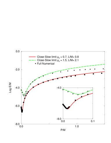
FIG. 2.: Energy as a function of initial momentum. Here $E$ is the energy radiated during coalescence, $P$ is the initial momentum, and $M$ is the initial ADM mass. Curves shown are for fixed parameter $\mu_{0}$, corresponding to separation of the holes in conformal space. The curves clearly show the “dip” effect, and the good agreement, even for large values of the momentum.

In Fig. 2, we plot the radiated energy computed from (16) for several values of initial separation $\mu_{0}$, and for a wide range of $P/M$ . On this plot, also, are presented the results for radiated energy from numerical results computations which make no approximations. The agreement between the numerical results and the results of the approximation is remarkably good, even at rather large values of $P/M$.

IV Results

Two features of Fig. 2 stand out. The first is “momentum dominance”: the radiated energy is dominated by the third integral in (15) unless the momentum is very small. The second obvious feature is that the approximation method works very well even for sizeable values of $P/M$.

To understand the implications of these features, let us start by reviewing the difference between the exact, nonlinear numerical computation, and the approximation scheme of Sec. III. In the exact method we start with an exact solution to the initial value equations described by two parameters, one a dimensionless measure of the separation of the holes, the other a dimensionless measure of the momentum. The process of generating the solution consists of four steps: (i) One starts with a very simple prescription for $\widehat{K}_{ab}$ constructed by superposing two solutions of form (5) corresponding to two coordinate positions in the conformally flat space. (ii) Equation (4) is then solved for the conformal factor and hence for the three geometry. (iii) The solution for the extrinsic curvature and the initial geometry is then “symmetrized” by an iterative process equivalent to adding image charges. (iv) This solution is numerically evolved off the initial hypersurface with the full nonlinear Einstein equations.

By contrast, the steps for the approximate solution are: (i) The (conformal) extrinsic curvature is taken to be the unsymmetrized superposition of two contributions with the form of (5). (ii) The conformal factor, and therefore the three geometry, is taken to be the symmetrized solution corresponding to throats located at the same points in the conformally flat space as the points in $\widehat{K}_{ab}$. (iii) This approximate initial data is then treated as initial data for the nonspherical perturbations of a Schwarzschild hole, and the perturbations are evolved with the linearized Einstein equations.

The difference in evolution off the initial hypersurface (full Einstein equations in one case, linearized equations in the other) is not a major source of error in the interesting cases, those with high momentum. As momentum increases, the location of the horizon in the initial geometry moves outward. The high momentum cases, therefore, correspond to throats which, on the initial hypersurface, are well inside an all-encompassing horizon. This is the situation in which the “close-limit” approximation method should work very well. It is also not surprising that no large error is introduced by the failure, in the approximation method, to symmetrize the extrinsic curvature. One way of understanding this is to note that $\psi_{\rm Mom}$ lacks the “image” contributions needed for symmetrization. These images only influence the form of $\widehat{K}_{ab}$ very close to the holes. As the separation between the holes gets smaller the horizon moves further from the throats and the effect of the images on $\widehat{K}_{ab}$ outside the horizon diminishes. We have checked numerically that the difference between the symmetrized and unsymmetrized $\widehat{K}_{ab}$, for all cases considered, is negligibly small outside the horizon.

These two aspects of the approximation method rely on the throats being “close” in some sense, an approximation that seems well justified. What remains to be explained is how the slow-limit approximation does such a good job of approximating the very “unslow” correct initial data. We must also justify the apparent inconsistency in how the approximation scheme deals with orders of $P$. In the computation of $\psi$ the scheme explicitly omits corrections of order $P^{2}$ in (4). Formally, then, we should only be able to keep terms of first order in $P$ in (15). But it is the apparently inconsistent $P^{2}$ terms, of course, which dominate at most points in Fig. 2 (“momentum dominance” in generation of radiation). Not only do the $P^{2}$ terms agree with the results of numerical relativity, but the agreement remains good for rather high values of $P/M$. This raises the question: just what momentum contributions has our approximation really omitted?

The momentum enters into the construction of the initial data in only two direct ways. First, it is an overall scaling parameter for $\widehat{K}_{ab}$. The expression in (7) is an approximation for small $L$, but it is exact in $P$. The process of symmetrizing does not change this. Up to a conformal factor, then, the extrinsic curvature is exactly linear in $P$. Second, $P$ enters the determination of the conformal factor through (4). The success of the slow approximation must be directly ascribed to the relatively unimportant role played by the right hand side of (4).

Further work will be needed for a real understanding of this, but some reasonable speculations can already be made. Due to momentum dominance the details of the initial three geometry are not crucial, so any quadrupolar distortion induced by $\widehat{K}_{ab}$ at large $P$ will be insignificant compared to the radiation generated by the extrinsic curvature. The “slow” approximation, of course, is not perfect; at sufficiently high momentum it begins to fail. We speculate that the reason for this failure is not primarily due to $\widehat{K}_{ab}$ generating quadrupolar distortions of the initial three geometry. Rather, it is the effect of that source on the monopole part of the conformal factor, and hence on the ADM mass “$M$,” that is used to scale physical quantities. When we do a comparison in Fig. 2 between the numerical relativity results and those of the approximation, we are comparing two cases for the same $\mu_{0}$ (i.e., the same coordinate separation in conformal space) and for the two cases we compare $E/M$ at a given value of $P/M$. We are therefore placing on an equal footing the true value of $M$ in the numerical relativity solution, and the $P\rightarrow 0$ value of $M$ in the approximation. It should be possible, in principle, to correct for this and, in effect, reduce the approximation to one in which we have only ignored the quadrupolar part of the source in (4).

The present results greatly help us to understand the success of the results of Ref. [7]. That

FIG. 3.: Radiated energy as a function of time for two different initial value sets. The first is for equal mass holes falling from rest at $\mu_{0}=2.2$. The second shows the result of a boosted collision starting from a separation parameter $\mu_{0}=1.406$ and a momentum $P/M=0.23$. The second set of initial data can be considered to be an approximation to a constant $t$ slice of the spacetime that evolves from the first set. The time scale is the (flat space) retarded time with zero corresponding to the time of apparent horizon formation. The energy scale of the $\mu_{0}=2.2$ curve has been offset to zero at the time of apparent horizon formation.

success seems to require two things about the generation of gravitational radiation in collisions from large distances: (i) There must be negligible radiation during the early motion, when the holes are in each other’s weak field region. (ii) The only important consequence of the early, weak-field, motion must be to give the holes momentum when each reaches the strong field region of the other. The first requirement is relatively easy to check. In Fig. 3 we plot radiated energy, computed by methods of numerical relativity, as a function of time, first for initial data representing two black holes falling from large separation. (The oscillations are due to the fact that almost all the energy comes off as “quasinormal ringing” of the final hole formed.) We also show the result of a second calculation. Cook[17] initial data are taken corresponding to the separation and momentum that the black holes would have after falling to a fairly close separation. A comparison of the curves verifies that the early stage of motion does not produce a significant contribution to the total outgoing radiation.

Our present results, and in particular momentum dominance, strongly support the second requirement for the success of the ideas of Ref. [7]. Since $\psi_{\rm Mom}$ is the source of essentially all the radiation, one can see that what is important about the early stages of the coalescence is only the development of extrinsic curvature. This does not, of course, explain why there seems to be insensitivity to the details of the extrinsic curvature. (Surely, the Bowen-York extrinsic curvature, symmetrized or not, is not actually the extrinsic curvature that evolves from earlier stationary conditions. Yet, it seems to be adequate to give good predictions.) A more satisfactory answer to this question means that we must understand the relationship between data on an initial hypersurface and how this evolves to data on subsequent hypersurfaces. We must also understand the importance of confining ourselves to conformally flat data on hypersurfaces. Progress on these questions will probably require comparable results from four distinct classes of initial data sets. These are (a) Misner data with large hole separation, (b) the non conformally-flat data with close holes that evolves from (a), (c) boosted conformally-flat data with close holes, and (d) boosted conformally-flat data in the close-slow approximation. In addition, one requires reasonable measures of physical separation and momentum so that correspondence can be drawn between disparate initial data sets.

There is strong motivation for carrying out such studies. The results so far achieved, both by numerical relativity and with the close and the slow approximation, are limited to head-on collisions. The situation of astrophysical interest, of course, is very different: the coalescence of orbiting holes. If the last few orbits in a coalescence are to be studied with numerical relativity, it will be crucial to understand what initial data are to be used to start the computation. Studies with the head-on collision provide a useful starting point to understanding the sensitivity of the radiation generation to the details of the initial data.

A rather different, and more speculative, motivation for a better understanding of these issues, is the hope that our approximation methods might be as successful with orbital problems as with head-on coalescence. These results might provide “easy” approximate answers over a reasonable range of orbital coalescences, and may therefore serve as a guide to the numerical studies.

- [1] Proceedings of the November 1994 meeting of the Grand Challenge Alliance to study black hole collisions may be obtained by contacting E. Seidel (unpublished).
- [2] A. A. Abramovici et al., Science 256, 325 (1992); K. S. Thorne, submitted to Proceedings of Snowmass 94 Summer Study on Particle and Nuclear Astrophysics and Cosmology, eds. W. W. Kolb and R. Peccei (World Scientific, Singapore).
- [3] A. Abrahams, R. Price, Phys. Rev. D53, 1963 (1996).
- [4] R. Price, J. Pullin, Phys. Rev. Lett. 72, 3297 (1994).
- [5] P. Anninos, R. H. Price, J. Pullin, E. Seidel and W.-M. Suen, Phys. Rev. D 52, 4462 (1995).
- [6] A. Abrahams, R. Price, Phys. Rev. D53, 1972 (1996).
- [7] A. M. Abrahams and G. B. Cook, Phys. Rev. D 50, R2364 (1994).
- [8] J. Bowen, J. York, Phys. Rev. D21, 2047 (1980).
- [9] L. L. Smarr, Ph.D. dissertation, University of Texas at Austin, unpublished (1975);
- [10] P. Anninos, D. Hobill, E. Seidel, L. Smarr, W.-M. Suen, Phys. Rev. Lett. 71, 2851 (1993); Phys. Rev. D 52, 2044 (1995)
- [11] C. Misner, Phys. Rev. 118, 1110 (1960).
- [12] A. Čadež, Ph.D. thesis, University of North Carolina at Chapel Hill, 1971.
- [13] P. Anninos et al., Technical Report No. 24, National Center for Supercomputing Applications (unpublished).
- [14] L. S. Anil D. Kulkarni and J. York, Physics Letters 96A, 228 (1983).
- [15] G. Cook, Ph.D. thesis, University of North Carolina at Chapel Hill, Chapel Hill, North Carolina, 1990.
- [16] G. B. Cook, M. W. Choptuik, M. R. Dubal , Phys. Rev. D 47, 1471 (1993); G. B. Cook, Phys. Rev. D 50, 5025 (1994).
- [17] G. B. Cook, Phys. Rev. D 44, 2983 (1991).
- [18] J. Pullin, “Colliding black holes with linearized gravity”, to appear in Fields Institute Communications, gr-qc/9508026.