\jl

6

The complete spectrum of the area from recoupling theory in loop quantum gravity

Simonetta Frittelli111e-mail: simo@artemis.phyast.pitt.edu    Luis Lehner222e-mail: luisl@artemis.phyast.pitt.edu and Carlo Rovelli333e-mail: rovelli@pitt.edu Department of Physics and Astronomy, University of Pittsburgh, Pittsburgh, PA 15260, USA.
(May 13, 1996)
Abstract

We compute the complete spectrum of the area operator in the loop representation of quantum gravity, using recoupling theory. This result extends previous derivations, which did not include the “degenerate” sector, and agrees with the recently computed spectrum of the connection-representation area operator.

1 Introduction

One of the central results of the loop approach to quantum gravity [1] is the derivation of discrete properties of spacetime geometry [2, 3, 4, 5, 6]. This derivation realizes the old idea [7] that spacetime might exhibit some kind of quantum discreteness at the Planck scale [8]. One of the manifestations of such discreteness is the fact that the operators associated to physical area and volume have discrete spectra [3]. This fact leads to the prediction that measurements of areas and volumes at the Planck scale would yield quantized values [4]. The explicit computation of the spectra of area and volume is thus a relevant step towards understanding the physics of the quantum gravitational field. Partial results on these spectra, for instance, have already been employed in discussing quantum gravitational corrections of black hole radiation [9] and black hole entropy [10].

Here, we consider the area operator. A regularization technique for the definition of this operator was introduced in [2], where some of the eigenvalues were computed. A more complete treatment was given in [3], where the spectrum was computed in full except for a “degenerate” sector formed by the states in which vertices or edges of the spin network lie on the surface. It is difficult to treat this degenerate sector –whose existence was pointed out by A Ashtekar– using the original regularization, because additional divergences appear. As a result, earlier works on the calculation of geometry eigenvalues in the loop representation exhibit incomplete spectra for the area operator. In this paper we introduce an alternative regularization, whose action is well defined on every loop state. This is done in Section 2. This regularization allows us to compute the full spectrum of the area operator. The computation is performed in Section 3, using recoupling theory, which provides a powerful computation technique in quantum gravity [5]. Our calculation here is a further proof of the effectiveness of recoupling theory in this context.

The complete spectrum of the area has been recently computed in Ref. [6] in the connection representation of quantum gravity [11]. The spectrum we obtain here fully agrees with the one given in Ref. [6]. Notice that the two representations are unitarily isomorphic, as argued by Lewandowski [12], and, recently, by DePietri [13], but the regularization techniques employed to define physical operators differ, so that the agreement is a non-trivial result.

2 The area operator

Consider a two-dimensional surface $\Sigma$ embedded in a three-dimensional metric manifold $M$. Let $\sigma^{u}$, $u=1,2$, be coordinates on $\Sigma$, $x^{a}$, $a=1,2,3$, coordinates on $M$, and let $x^{a}(\sigma^{u})$ represent the embedding. If we represent the metric of $M$ by means of the inverse densitized triad $\tilde{E}^{ai}$, the area of $\Sigma$ is given by

$$A[\Sigma]=\int_{\Sigma}d^{2}\sigma\,\sqrt{\tilde{E}^{ai}\tilde{E}^{b}_{i}\,n_{a}n_{b}}$$ (1)

where $n_{a}=\frac{1}{2}\epsilon_{abc}\frac{\partial x^{b}}{\partial\sigma^{1}}\frac{\partial x^{c}}{\partial\sigma^{2}}$ is the one-form normal to $\Sigma$. Since the metric of physical space is the gravitational field, $A[\Sigma]$ is a function of the gravitational field: it is then represented by a quantum operator $\hat{A}[\Sigma]$ in a quantum description of gravity. In the loop quantization of general relativity, one constructs $\hat{A}[\Sigma]$ by expressing the area in terms of loop variables and then replacing the loop variables with the corresponding quantum loop operators. Since (1) involves products of two triads $\tilde{E}^{a}$, the area is expected to be a function of the loop variable of order 2 (with two “hands”)

$${\cal T}^{ab}[\alpha](\mbox{\boldmath$x$},\mbox{\boldmath$y$})=-\mbox{Tr}[U_{\alpha}(\mbox{\boldmath$y$},\mbox{\boldmath$x$})\tilde{E}^{a}(\mbox{\boldmath$x$})U_{\alpha}(\mbox{\boldmath$x$},\mbox{\boldmath$y$})\tilde{E}^{b}(\mbox{\boldmath$y$})]$$ (2)

where $\alpha$ denotes a loop and $U_{\alpha}(\mbox{\boldmath$x$},\mbox{\boldmath$y$})$ is the parallel propagator of the Ashtekar connection along $\alpha$ with end points at $x$ and $y$. Throughout this work, we assume familiarity with the loop representation [1]; in particular, we refer reader to [5] for notations and conventions. (Notice that we deal here with conventional loop quantum gravity, not with its quantum SU(2) deformations [14].)

A direct change of variables $\tilde{E}^{a}\,\tilde{E}^{b}\rightarrow{\cal T}^{ab}$ leads to an expression which is not suitable for quantization, due to the the presence of products of operators at the same point. Therefore a regularization procedure is needed in order to define $\hat{A}[\Sigma]$. This can be done by selecting a sequence of quantities $A_{\epsilon}[\Sigma]$ converging to (1) when $\epsilon$ goes to zero, each of which does not involve products of variables at the same point. The sequence can be quantized by substituting the dynamical variables with the corresponding quantum operators. The operator $\hat{A}(\Sigma)$ is then defined as a suitable operator limit of the resulting sequence of operators. There is a degree of arbitrariness in any regularization procedure (in conventional field theory: dimensional regularization, point splitting, Pauli-Villar…). In the present context, the regularization procedure must satisfy two requirements. First, the classical regularized expression must converge to the correct classical quantity (the area) when the regulator is removed; second, the quantum operator must be well defined in the limit and must respect the invariances of the theory; in particular, the operator should transform correctly under diffeomorphisms. Contrary to a possible impression that the choice of a regularization leaves great arbitrariness, implementing both requirements is actually far from trivial. The modification of the regularization procedure for the area operator considered in this paper is forced by the realization that the regularization considered in [3] fails to satisfy the second viability criterion, if one relaxes the simplifying choice of neglecting certain states. In the following, we construct one such regularization of the area operator.

Let us begin by introducing a smooth coordinate $\tau$ over a finite neighborhood of $\Sigma$, in such a way that $\Sigma$ is given by $\tau=0$. Consider then the three-dimensional region around $\Sigma$ defined by $-\delta/2\leq\tau\leq\delta/2$. Partition this region into a number of blocks $\cal D_{I}$ of coordinate height $\delta$ and square horizontal section of coordinate side $\epsilon$. For each fixed choice of $\epsilon$ and $\delta$, we label the blocks by an index $I$. Later, we will send both $\delta$ and $\epsilon$ to zero. In order to have a one-parameter sequence, we now choose $\delta$ as a fixed function of $\epsilon$. For technical reasons, the height of the block $\cal D_{I}$ must decrease more rapidly than $\epsilon$ in the limit; thus, we put $\delta=\epsilon^{k}$ with any $k$ greater than 1 and smaller than 2.

Consider one of the blocks. The intersection of the block and a $\tau=constant$ surface is a square surface: let $A_{I}(\tau)$ be the area of such surface. Let $A_{I\epsilon}$ be the average over $\tau$ of the areas of the surfaces in the block. Namely

$$A_{I\epsilon}\equiv\frac{1}{\delta}\int^{\delta/2}_{-\delta/2}A_{I}(\tau)d\tau=\frac{1}{\delta}\int_{{\cal D_{I}}}d^{3}\!x\;\sqrt{\tilde{E}^{ai}\tilde{E}^{b}_{i}n_{a}n_{b}}\;\;.$$ (3)

Summing over the blocks yields the average of the areas of the $\tau=constant$ surfaces, and as $\epsilon$ (and therefore $\delta$) approaches zero, the sum converges to the area of the surface $\Sigma$. Therefore we have

$$A[\Sigma]=\lim_{\epsilon\to 0}\sum_{I}A_{I\epsilon}\equiv\lim_{\epsilon\to 0}A_{\epsilon}[\Sigma].$$ (4)

The quantity $A_{I\epsilon}$ associated to each block can be expressed in terms of the fundamental loop variables as follows. First, let us pick an arbitrary fiducial background coordinate system. For every two points $x$ and $y$, let $\alpha$ be a loop determined by $x$ and $y$ – say as the zero-area loop obtained by following back and forth a straight segment between $x$ and $y$, in the fiducial coordinate system. Then, we write

$$A_{I\epsilon}=\sqrt{A_{I\epsilon}^{2}}$$ (5)

and notice that

$$A_{I\epsilon}^{2}=\frac{1}{2\delta^{2}}\int_{{\cal D}\otimes{\cal D}}d^{3}x\,d^{3}y\;n_{a}(\mbox{\boldmath$x$})n_{b}(\mbox{\boldmath$y$}){\cal T}^{ab}[\alpha](\mbox{\boldmath$x$},\mbox{\boldmath$y$})\;+\;O(\epsilon^{5}).$$ (6)

Equation (6) holds because of the following. We have

$${\cal T}^{ab}[\alpha](\mbox{\boldmath$x$},\mbox{\boldmath$y$})=2\tilde{E}^{ai}(\mbox{\boldmath$x$}_{I})\tilde{E}^{b}_{i}(\mbox{\boldmath$x$}_{I})+O(\epsilon)$$ (7)

for any three points $x$, $y$, and $\mbox{\boldmath$x$}_{I}$, in ${\cal D}$. It follows that

$\displaystyle\fl\epsilon^{4}\,n_{a}(\mbox{\boldmath$x$}_{I})n_{b}(\mbox{\boldmath$x$}_{I})\tilde{E}^{ai}(\mbox{\boldmath$x$}_{I})\tilde{E}^{b}_{i}(\mbox{\boldmath$x$}_{I})$
$\displaystyle\lo=\frac{1}{2\delta^{2}}\int_{{\cal D}\otimes{\cal D}}d^{3}\!x\,d^{3}\!y\;n_{a}(\mbox{\boldmath$x$})n_{b}(\mbox{\boldmath$y$}){\cal T}^{ab}[\alpha](\mbox{\boldmath$x$},\mbox{\boldmath$y$})\;+\;O(\epsilon^{5}).$ (8)

Since

$\displaystyle A_{I\epsilon}^{2}$ $\displaystyle=$ $\displaystyle\bigg{(}\frac{1}{\delta}\int^{\delta/2}_{-\delta/2}A_{I\epsilon}(\tau)d\tau\bigg{)}^{2}$ (9)
$\displaystyle=$ $\displaystyle\bigg{(}\frac{1}{\delta}\int_{{\cal D}}d^{3}\!x\;\sqrt{\tilde{E}^{ai}\tilde{E}^{b}_{i}n_{a}n_{b}}\bigg{)}^{2}$
$\displaystyle=$ $\displaystyle\epsilon^{4}\,n_{a}(\mbox{\boldmath$x$}_{I})n_{b}(\mbox{\boldmath$x$}_{I})\tilde{E}^{ai}(\mbox{\boldmath$x$}_{I})\tilde{E}^{b}_{i}(\mbox{\boldmath$x$}_{I})\;+\;O(\epsilon^{5}),$

Equation (6) follows.

Equations (4), (5) and (6) define our regularization for the area. The operator $\hat{A}[\Sigma]$ can now be defined as

$\displaystyle\hat{A}[\Sigma]\equiv\lim_{\epsilon\to 0}\hat{A}_{\epsilon}[\Sigma],$ (10)
$\displaystyle\mbox{with}\hskip 11.38092pt\hat{A}_{\epsilon}[\Sigma]\equiv\sum_{I}\sqrt{\hat{A^{2}_{I\epsilon}}},$ (11)
$\displaystyle\mbox{and}\hskip 19.91684pt\hat{A^{2}_{I\epsilon}}\equiv\frac{1}{2\delta^{2}}\int_{{\cal D}\otimes{\cal D}}d^{3}\!x\,d^{3}\!y\;n_{a}(\mbox{\boldmath$x$})n_{b}(\mbox{\boldmath$y$})\hat{\cal T}^{ab}[\alpha](\mbox{\boldmath$x$},\mbox{\boldmath$y$}).$ (12)

The meaning of the operator limit in (10) is discussed in [5].

The space of states of the quantum theory is the space of loops up to the Mandelstam relations (which essentially identify loops with the same holonomy). A state is usually denoted $\langle\beta|$ (for the Mandelstam class of the loop $\beta$) or by means of a bracketed pictorial representation of the loop $\beta$. Any state has an associated graph, which is characterized as a collection of edges (smooth lines of generic multiplicity) and vertices (points at which lines converge). A vertex has a valence, defined as the number of edges converging to it. A graph is said to be $n$-valent if all its vertices have valence $n$ or less. A convenient basis of the space of quantum states is the spin network basis, introduced in [16] and further discussed in [5]. Spin network states are given by the linear combinations of loop states obtained by antisymmetrizing the loops along each edge of their graphs. Because of the Mandelstam relations, these linear combinations form a complete basis. A spin network is characterized by an $n$-valent graph, an assignment of an ordering to the edges converging to each vertex, a color $p$ assigned to each edge (the number of antisymmetrized loops), and a color $v$ assigned to each vertex (characterizing the rooting of the loops through the vertex). An $n$-valent spin network can be expanded into a “virtual” trivalent spin network, lying in the ribbon associated to the state – a possibility that we exploit below. See [5] for details.

The action of $\hat{A}[\Sigma]$ on the quantum states is found from the action of the $\hat{\cal T}^{ab}[\alpha]$ operators, which we recall here. The operator $\hat{\cal T}^{ab}[\alpha](\mbox{\boldmath$x$},\mbox{\boldmath$y$})$ annihilates the state $\langle\beta|$ unless the loop $\beta$ intersects the loop $\alpha$ at the points $x$ and $y$. If the loops do intersect as needed, the action of the operator on the state gives the (Mandelstam class of) the union of the loops $\beta$ and $\alpha$, with two additional vertices at the points $x$ and $y$. More precisely, if $x$ and $y$ fall over two edges of $\beta$ with color $p$ and $q$ respectively, we have

 pq|𝒯^ab[α](𝒙,𝒚)=l04pqΔa[β,𝒙]Δb[β,𝒚] 2pqxy|bra pqsuperscript^𝒯𝑎𝑏delimited-[]𝛼𝒙𝒚superscriptsubscript𝑙04𝑝𝑞superscriptΔ𝑎𝛽𝒙superscriptΔ𝑏𝛽𝒚bra 2pqxy\Bigg{\langle}\!\!\!\!\!\!\!\!{\begin{array}[]{c}\mbox{ {{\begin{picture}(15.0,20.0){{ \put(9.5,14.0){\line(1,0){5.1}} \put(15.0,14.0){\line(1,0){1.0}} \put(17.0,14.0){\line(1,0){1.0}} \put(6.0,14.0){\line(1,0){1.0}} \put(8.0,14.0){\line(1,0){1.0}} \put(9.5,6.0){\line(1,0){5.1}} \put(15.0,6.0){\line(1,0){1.0}} \put(17.0,6.0){\line(1,0){1.0}} \put(6.0,6.0){\line(1,0){1.0}} \put(8.0,6.0){\line(1,0){1.0}} \put(11.5,12.0){${\scriptscriptstyle p}$} \put(11.5,7.0){${\scriptscriptstyle q}$} }} \end{picture}}}}\end{array}}\,\,\>\Bigg{|}\hat{\cal T}^{ab}[\alpha](\mbox{\boldmath$x$},\mbox{\boldmath$y$})=-l_{0}^{4}\,p\,q\,\Delta^{a}[\beta,\mbox{\boldmath$x$}]\,\Delta^{b}[\beta,\mbox{\boldmath$y$}]\Bigg{\langle}\!\!\!\!\!\!\!\!{\begin{array}[]{c}\mbox{ {{\begin{picture}(15.0,20.0){{ \put(9.5,14.0){\line(1,0){5.1}} \put(15.0,14.0){\line(1,0){1.0}} \put(17.0,14.0){\line(1,0){1.0}} \put(6.0,14.0){\line(1,0){1.0}} \put(8.0,14.0){\line(1,0){1.0}} \put(9.5,6.0){\line(1,0){5.1}} \put(15.0,6.0){\line(1,0){1.0}} \put(17.0,6.0){\line(1,0){1.0}} \put(6.0,6.0){\line(1,0){1.0}} \put(8.0,6.0){\line(1,0){1.0}} \put(12.0,6.0){\line(0,1){8.0}} \put(13.5,10.0){${\scriptscriptstyle 2}$} \put(9.1,12.2){${\scriptscriptstyle p}$} \put(9.1,6.8){${\scriptscriptstyle q}$} \put(12.0,6.0){\circle*{1.0}} \put(12.0,14.0){\circle*{1.0}} \put(11.2,14.9){$\mbox{\boldmath{$\scriptscriptstyle x$}}$ } \put(11.2,4.0){$\mbox{\boldmath{$\scriptscriptstyle y$}}$} }} \end{picture}}}}\end{array}}\,\,\>\Bigg{|} (13)

where

$$\Delta^{a}[\beta,\mbox{\boldmath$x$}]=\int_{\beta}d\tau~{}\dot{\beta}^{a}(\tau)\delta^{3}[\beta(\tau),\mbox{\boldmath$x$}].$$ (14)

In the picture, the loop $\alpha$ is represented as a double line running back and forth between the intersection points $x$ and $y$ (the two “grasps”), hence the label 2.

3 Spectrum of the area operator

In this section we discuss the action of the operator $\hat{A}[\Sigma]$ on a generic spin network state $\langle\ S\>|$. Due to the limiting procedure involved in its definition, the operator $\hat{A}[\Sigma]$ does not affect the graph of any state. Furthermore, since the action of $\hat{\cal T}^{ab}$ inside a specific coordinate block ${\cal D}$ vanishes unless the graph of the state intersects ${\cal D}$, the action of $\hat{A}[\Sigma]$ ultimately consists of a sum of numerable terms, one for each intersection $i$ of the graph with the surface. Here we allow for spin networks having vertices on $\Sigma$ or edges tangential to $\Sigma$, unlike previous treatments of this problem [5].

Consider an intersection $i$ between the spin network and the surface. For the purpose of this discussion, we can consider a generic point on an edge as a “two-valent vertex”, and thus say, without loss of generality, that $i$ is a vertex. In general, there will be $n$ edges emerging from $i$. Some of these will emerge above, some below and some tangentially to the surface $\Sigma$. Since we are taking the limit in which the blocks shrink to zero, we may assume, without loss of generality that the surface and the edges are linear around $i$ (see below for subtleties concerning higher derivatives). Due to the two integrals in (12), the position of two hands of the area operator are integrated over each block. As the action of $\hat{\cal T}^{ab}$ is non-vanishing only when both hands fall on the spin network, we obtain $n^{2}$ terms, one for every couple of grasped edges. Consider one of these terms, in which the grasped edges have color $p$ and $q$. The state

 pq2i|ϵsubscriptbra pq2iitalic-ϵ\Bigg{\langle}\!\!\!\!\begin{array}[]{c}\mbox{ {{\begin{picture}(15.0,20.0){{ \put(8.0,8.0){\line(2,-1){7.0}} \put(8.0,8.0){\line(-3,5){4.5}} \put(6.8,10.0){\line(1,0){2.2}} \put(1.8,10.5){${\scriptstyle p}$} \put(12.0,3.0){${\scriptstyle q}$} \put(11.0,10.0){${\scriptstyle\scriptstyle{2}}$} \put(8.0,8.0){\circle*{1.5}} \put(6.0,6.0){${\scriptstyle i}$} \put(9.0,8.0){\oval(4.0,4.0)[tr]} \put(11.0,8.0){\line(0,-1){1.5}} \put(6.8,10.0){\circle*{1.0}} \put(11.0,6.5){\circle*{1.0}} }} \end{picture}}}}\end{array}\>\Bigg{|}_{\epsilon}\; (15)

represents, up to factors, the result of the action of $\hat{\cal T}^{ab}$ on the edges $p$ and $q$ of an $n$-valent intersection $i$. The irrelevant edges are not shown. The edges labeled $p$ and $q$ are generic, in the sense that their angles with the surface do not need to be specified at this point (the two edges may also be identical). From the definition (10-12) of the area operator and the definition (13-14) of the $\hat{\cal T}^{ab}$ operator, each term in which the grasps run over two edges of color $p$ and $q$ is of the form

\fl12δ2𝒟𝒟d3xd3yna(𝒙)Δa[β,𝒙]nb(𝒚)Δb[β,𝒚]pq pq2i|ϵ\fl12superscript𝛿2subscripttensor-product𝒟𝒟superscript𝑑3𝑥superscript𝑑3𝑦subscript𝑛𝑎𝒙superscriptΔ𝑎𝛽𝒙subscript𝑛𝑏𝒚superscriptΔ𝑏𝛽𝒚𝑝𝑞subscriptbra pq2iitalic-ϵ\displaystyle\fl\frac{1}{2\delta^{2}}\int_{{\cal D}\otimes{\cal D}}d^{3}\!x\,d^{3}\!y\;n_{a}(\mbox{\boldmath$x$})\Delta^{a}[\beta,\mbox{\boldmath$x$}]n_{b}(\mbox{\boldmath$y$})\Delta^{b}[\beta,\mbox{\boldmath$y$}]p\,q\;\Bigg{\langle}\!\!\!\!\begin{array}[]{c}\mbox{ {{\begin{picture}(15.0,20.0){{ \put(8.0,8.0){\line(2,-1){7.0}} \put(8.0,8.0){\line(-3,5){4.5}} \put(6.8,10.0){\line(1,0){2.2}} \put(1.8,10.5){${\scriptstyle p}$} \put(12.0,3.0){${\scriptstyle q}$} \put(11.0,10.0){${\scriptstyle\scriptstyle{2}}$} \put(8.0,8.0){\circle*{1.5}} \put(6.0,6.0){${\scriptstyle i}$} \put(9.0,8.0){\oval(4.0,4.0)[tr]} \put(11.0,8.0){\line(0,-1){1.5}} \put(6.8,10.0){\circle*{1.0}} \put(11.0,6.5){\circle*{1.0}} }} \end{picture}}}}\end{array}\>\Bigg{|}_{\epsilon} (17)
$\displaystyle\lo=\frac{1}{2\delta^{2}}\int_{{\cal D}\otimes{\cal D}}\Bigg{(}n_{a}(\mbox{\boldmath$x$})\int_{\beta}ds~{}\dot{\beta}^{a}(s)\delta^{3}[\beta(s),\mbox{\boldmath$x$}]$
×nb(𝒚)βdtβ˙b(t)δ3[β(t),𝒚]pq pq2i|ϵ)d3xd3y\displaystyle\times n_{b}(\mbox{\boldmath$y$})\int_{\beta}dt~{}\dot{\beta}^{b}(t)\delta^{3}[\beta(t),\mbox{\boldmath$y$}]\;p\,q\;\Bigg{\langle}\!\!\!\!\begin{array}[]{c}\mbox{ {{\begin{picture}(15.0,20.0){{ \put(8.0,8.0){\line(2,-1){7.0}} \put(8.0,8.0){\line(-3,5){4.5}} \put(6.8,10.0){\line(1,0){2.2}} \put(1.8,10.5){${\scriptstyle p}$} \put(12.0,3.0){${\scriptstyle q}$} \put(11.0,10.0){${\scriptstyle\scriptstyle{2}}$} \put(8.0,8.0){\circle*{1.5}} \put(6.0,6.0){${\scriptstyle i}$} \put(9.0,8.0){\oval(4.0,4.0)[tr]} \put(11.0,8.0){\line(0,-1){1.5}} \put(6.8,10.0){\circle*{1.0}} \put(11.0,6.5){\circle*{1.0}} }} \end{picture}}}}\end{array}\>\Bigg{|}_{\epsilon}\Bigg{)}d^{3}\!x\,d^{3}\!y\; (19)
\lo=12δ2β𝑑sna(s)β˙a(s)β𝑑tnb(t)β˙b(t)pq pq2i|ϵ\lo12superscript𝛿2subscript𝛽differential-d𝑠subscript𝑛𝑎𝑠superscript˙𝛽𝑎𝑠subscript𝛽differential-d𝑡subscript𝑛𝑏𝑡superscript˙𝛽𝑏𝑡𝑝𝑞subscriptbra pq2iitalic-ϵ\displaystyle\lo=\frac{1}{2\delta^{2}}\int_{\beta}ds\;n_{a}(s)~{}\dot{\beta}^{a}(s)\int_{\beta}dt\;n_{b}(t)~{}\dot{\beta}^{b}(t)p\,q\;\Bigg{\langle}\!\!\!\!\begin{array}[]{c}\mbox{ {{\begin{picture}(15.0,20.0){{ \put(8.0,8.0){\line(2,-1){7.0}} \put(8.0,8.0){\line(-3,5){4.5}} \put(6.8,10.0){\line(1,0){2.2}} \put(1.8,10.5){${\scriptstyle p}$} \put(12.0,3.0){${\scriptstyle q}$} \put(11.0,10.0){${\scriptstyle\scriptstyle{2}}$} \put(8.0,8.0){\circle*{1.5}} \put(6.0,6.0){${\scriptstyle i}$} \put(9.0,8.0){\oval(4.0,4.0)[tr]} \put(11.0,8.0){\line(0,-1){1.5}} \put(6.8,10.0){\circle*{1.0}} \put(11.0,6.5){\circle*{1.0}} }} \end{picture}}}}\end{array}\>\Bigg{|}_{\epsilon} (21)
\lo=pq2δ2(β𝑑sna(s)β˙a(s)β𝑑tnb(t)β˙b(t)) pq2i|+O(ϵ).\lo𝑝𝑞2superscript𝛿2subscript𝛽differential-d𝑠subscript𝑛𝑎𝑠superscript˙𝛽𝑎𝑠subscript𝛽differential-d𝑡subscript𝑛𝑏𝑡superscript˙𝛽𝑏𝑡bra pq2i𝑂italic-ϵ\displaystyle\lo=\frac{p\,q}{2\delta^{2}}\Bigg{(}\int_{\beta}ds\;n_{a}(s)~{}\dot{\beta}^{a}(s)\int_{\beta}dt\;n_{b}(t)~{}\dot{\beta}^{b}(t)\Bigg{)}\Bigg{\langle}\!\!\!\!\begin{array}[]{c}\mbox{ {{\begin{picture}(15.0,20.0){{ \put(8.0,8.0){\line(2,-1){7.0}} \put(8.0,8.0){\line(-3,5){4.5}} \put(6.8,10.0){\line(1,0){2.2}} \put(1.8,10.5){${\scriptstyle p}$} \put(12.0,3.0){${\scriptstyle q}$} \put(11.0,10.0){${\scriptstyle\scriptstyle{2}}$} \put(8.0,8.0){\circle*{1.5}} \put(6.0,6.0){${\scriptstyle i}$} \put(9.0,8.0){\oval(4.0,4.0)[tr]} \put(11.0,8.0){\line(0,-1){1.5}} \put(6.8,10.0){\circle*{1.0}} \put(11.0,6.5){\circle*{1.0}} }} \end{picture}}}}\end{array}\>\Bigg{|}+O(\epsilon)\;. (23)

The last step in the preceding calculation is pulling the state outside the integral sign. This is possible because the ϵitalic-ϵ\epsilon-dependent states  pq2i|ϵsubscriptbra pq2iitalic-ϵ\Bigg{\langle}\!\!\!\!\begin{array}[]{c}\mbox{ {{\begin{picture}(15.0,20.0){{ \put(8.0,8.0){\line(2,-1){7.0}} \put(8.0,8.0){\line(-3,5){4.5}} \put(6.8,10.0){\line(1,0){2.2}} \put(1.8,10.5){${\scriptstyle p}$} \put(12.0,3.0){${\scriptstyle q}$} \put(11.0,10.0){${\scriptstyle\scriptstyle{2}}$} \put(8.0,8.0){\circle*{1.5}} \put(6.0,6.0){${\scriptstyle i}$} \put(9.0,8.0){\oval(4.0,4.0)[tr]} \put(11.0,8.0){\line(0,-1){1.5}} \put(6.8,10.0){\circle*{1.0}} \put(11.0,6.5){\circle*{1.0}} }} \end{picture}}}}\end{array}\>\Bigg{|}_{\epsilon} all have the same limit state as ϵ0italic-ϵ0\epsilon\to 0, namely  pq2i|bra pq2i\Bigg{\langle}\!\!\!\!\begin{array}[]{c}\mbox{ {{\begin{picture}(15.0,20.0){{ \put(8.0,8.0){\line(2,-1){7.0}} \put(8.0,8.0){\line(-3,5){4.5}} \put(6.8,10.0){\line(1,0){2.2}} \put(1.8,10.5){${\scriptstyle p}$} \put(12.0,3.0){${\scriptstyle q}$} \put(11.0,10.0){${\scriptstyle\scriptstyle{2}}$} \put(8.0,8.0){\circle*{1.5}} \put(6.0,6.0){${\scriptstyle i}$} \put(9.0,8.0){\oval(4.0,4.0)[tr]} \put(11.0,8.0){\line(0,-1){1.5}} \put(6.8,10.0){\circle*{1.0}} \put(11.0,6.5){\circle*{1.0}} }} \end{picture}}}}\end{array}\>\Bigg{|}; i.e.,

 pq2i|ϵ= pq2i|+O(ϵ)subscriptbra pq2iitalic-ϵbra pq2i𝑂italic-ϵ\Bigg{\langle}\!\!\!\!\begin{array}[]{c}\mbox{ {{\begin{picture}(15.0,20.0){{ \put(8.0,8.0){\line(2,-1){7.0}} \put(8.0,8.0){\line(-3,5){4.5}} \put(6.8,10.0){\line(1,0){2.2}} \put(1.8,10.5){${\scriptstyle p}$} \put(12.0,3.0){${\scriptstyle q}$} \put(11.0,10.0){${\scriptstyle\scriptstyle{2}}$} \put(8.0,8.0){\circle*{1.5}} \put(6.0,6.0){${\scriptstyle i}$} \put(9.0,8.0){\oval(4.0,4.0)[tr]} \put(11.0,8.0){\line(0,-1){1.5}} \put(6.8,10.0){\circle*{1.0}} \put(11.0,6.5){\circle*{1.0}} }} \end{picture}}}}\end{array}\>\Bigg{|}_{\epsilon}=\Bigg{\langle}\!\!\!\!\begin{array}[]{c}\mbox{ {{\begin{picture}(15.0,20.0){{ \put(8.0,8.0){\line(2,-1){7.0}} \put(8.0,8.0){\line(-3,5){4.5}} \put(6.8,10.0){\line(1,0){2.2}} \put(1.8,10.5){${\scriptstyle p}$} \put(12.0,3.0){${\scriptstyle q}$} \put(11.0,10.0){${\scriptstyle\scriptstyle{2}}$} \put(8.0,8.0){\circle*{1.5}} \put(6.0,6.0){${\scriptstyle i}$} \put(9.0,8.0){\oval(4.0,4.0)[tr]} \put(11.0,8.0){\line(0,-1){1.5}} \put(6.8,10.0){\circle*{1.0}} \put(11.0,6.5){\circle*{1.0}} }} \end{picture}}}}\end{array}\>\Bigg{|}+O(\epsilon) (24)

and, hence, the substitution of the $\epsilon$-dependent states with their $\epsilon$-independent limit in the integral is possible up to terms of order $O(\epsilon)$. Note the following:

$\displaystyle\int_{\beta}dt\;n_{b}(t)~{}\dot{\beta}^{b}(t)=\left\{\begin{array}[]{l}0\hskip 28.45274pt\mbox{if $\beta$ is tangent to $\Sigma$}\\ \delta/2\hskip 28.45274pt\mbox{otherwise.}\end{array}\right.$ (27)

This result is independent of the angle the edge makes with the surface because $\delta$ can always be chosen sufficiently small so that $\beta$ crosses the top and bottom of the coordinate block $\cal D$ (this is the reason for requiring that $\delta$ goes to zero faster than $\epsilon$). Also, since we have chosen $k$ smaller than 2, it follows that any edge tangential to the surface exits the box from the side, irrespectively from its second (and higher) derivatives, for sufficiently small $\epsilon$, and gives a vanishing contribution as $\epsilon$ goes to zero. Thus, the parenthetic factor in (23) is either 00 or $\delta^{2}/4$ depending on whether one or none of the edges lies on the surface. Consequently, in the limit considered, the edges tangent to the surface do not contribute to the action of the area whereas every non vanishing term takes the form

l04pq8 pq2i|.superscriptsubscript𝑙04𝑝𝑞8bra pq2i-\frac{l_{0}^{4}\,p\,q}{8}\Bigg{\langle}\!\!\!\!\begin{array}[]{c}\mbox{ {{\begin{picture}(15.0,20.0){{ \put(8.0,8.0){\line(2,-1){7.0}} \put(8.0,8.0){\line(-3,5){4.5}} \put(6.8,10.0){\line(1,0){2.2}} \put(1.8,10.5){${\scriptstyle p}$} \put(12.0,3.0){${\scriptstyle q}$} \put(11.0,10.0){${\scriptstyle\scriptstyle{2}}$} \put(8.0,8.0){\circle*{1.5}} \put(6.0,6.0){${\scriptstyle i}$} \put(9.0,8.0){\oval(4.0,4.0)[tr]} \put(11.0,8.0){\line(0,-1){1.5}} \put(6.8,10.0){\circle*{1.0}} \put(11.0,6.5){\circle*{1.0}} }} \end{picture}}}}\end{array}\>\Bigg{|}. (28)

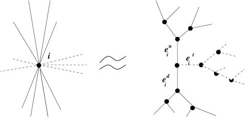
Generically, there will be several edges above, below, and tangential to the surface $\Sigma$. Following [5], we now expand the vertex $i$ into a virtual trivalent spin network. We choose to perform the expansion in such a way that all edges above the surface converge to a single “principal” virtual edge $e^{u}$; all edges below the surface converge to a single principal virtual edge $e^{d}$; and all edges tangential to the surface converge to a single principal virtual edge $e^{t}$. The three principal edges join in the principal trivalent vertex. This trivalent expansion is shown in Figure 1. This choice simplifies the calculation of the action of the area, since the sum of the grasps of one hand on all real edges above the surface is equivalent to a single grasp on $e^{u}$ (and similarly for the edges below the surface and $e^{d}$). This follows from the identity

p pqr2+q pqr2=r pqr2,𝑝 pqr2𝑞 pqr2𝑟 pqr2p\!\!\!\!\!\begin{array}[]{c}\mbox{ {{\begin{picture}(15.0,20.0){{ \put(10.0,10.0){\line(0,-1){5.0}} \put(10.0,10.0){\line(1,1){4.0}} \put(10.0,10.0){\line(-1,1){4.0}} \put(8.0,12.0){\line(-1,0){3.5}} \put(7.5,13.5){${\scriptscriptstyle p}$} \put(12.0,13.5){${\scriptscriptstyle q}$} \put(10.0,5.5){${\scriptscriptstyle r}$} \put(5.2,12.5){${\scriptscriptstyle 2}$} \put(8.0,12.0){\circle*{1.0}} }} \end{picture}}}}\end{array}+q\!\!\!\!\!\begin{array}[]{c}\mbox{ {{\begin{picture}(15.0,20.0){{ \put(10.0,10.0){\line(0,-1){5.0}} \put(10.0,10.0){\line(1,1){4.0}} \put(10.0,10.0){\line(-1,1){4.0}} \put(12.5,12.5){\line(-1,0){3.0}} \put(7.5,13.5){${\scriptscriptstyle p}$} \put(12.0,13.5){${\scriptscriptstyle q}$} \put(10.0,5.5){${\scriptscriptstyle r}$} \put(10.0,12.8){${\scriptscriptstyle 2}$} \put(12.5,12.5){\circle*{1.0}} }} \end{picture}}}}\end{array}=r\!\!\!\!\!\begin{array}[]{c}\mbox{ {{\begin{picture}(15.0,20.0){{ \put(10.0,10.0){\line(0,-1){5.0}} \put(10.0,10.0){\line(1,1){4.0}} \put(10.0,10.0){\line(-1,1){4.0}} \put(10.0,8.0){\line(-1,0){3.5}} \put(7.5,13.5){${\scriptscriptstyle p}$} \put(12.0,13.5){${\scriptscriptstyle q}$} \put(10.0,5.5){${\scriptscriptstyle r}$} \put(8.0,8.8){${\scriptscriptstyle 2}$} \put(10.0,8.0){\circle*{1.0}} }} \end{picture}}}}\end{array}, (29)

which can be proven as follows. Using the recoupling theorem (63), the left hand side of (29) can be written as

j(p{2pjqrp}qλj2r{rpjq2q}) 2prqjsubscript𝑗𝑝2𝑝𝑗𝑞𝑟𝑝𝑞subscriptsuperscript𝜆2𝑟𝑗𝑟𝑝𝑗𝑞2𝑞 2prqj\sum_{j}\Bigg{(}p\,{\left\{\begin{array}[]{ccc}2&p&j\\ q&r&p\end{array}\right\}}-q\,\lambda^{2r}_{j}{\left\{\begin{array}[]{ccc}r&p&j\\ q&2&q\end{array}\right\}}\Bigg{)}\begin{array}[]{c}\mbox{ {{\begin{picture}(40.0,50.0){ \put(0.0,0.0){$2$}\put(0.0,40.0){$p$} \put(35.0,0.0){$r$}\put(35.0,40.0){$q$} \put(10.0,10.0){\line(1,1){10.0}}\put(10.0,40.0){\line(1,-1){10.0}} \put(20.0,30.0){\line(1,1){10.0}}\put(20.0,20.0){\line(1,-1){10.0}} \put(20.0,20.0){\line(0,1){10.0}}\put(22.0,22.0){$j$} \put(20.0,20.0){\circle*{3.0}}\put(20.0,30.0){\circle*{3.0}} } \end{picture}}}}\end{array} (30)

where $j$ can take the values $r-2$, $r$ and $r+2$. A straightforward calculation making use of (56) gives

$$p\,{\left\{\begin{array}[]{ccc}2&p&j\\ q&r&p\end{array}\right\}}-q\,\lambda^{2r}_{j}{\left\{\begin{array}[]{ccc}r&p&j\\ q&2&q\end{array}\right\}}=r\,\delta_{jr}.$$ (31)

Thus, (29) follows. A repeated application of the identity (29) allows us to slide all graspings from the real edges down to the two virtual edges $e^{u}$ and $e^{d}$. Thus, each intersection contributes as a single principal trivalent vertex, regardless of its valence.

We are now in position to calculate the action of the area on a generic intersection. From the discussion above, the only relevant terms are as follows

\fl qpr|A^i2\flbra qprsubscriptsuperscript^𝐴2𝑖\displaystyle\fl\Bigg{\langle}\!\!\!\!\begin{array}[]{c}\mbox{ {{\begin{picture}(15.0,20.0){{ \put(6.0,0.0){\line(0,1){16.0}} \put(6.0,8.0){\line(1,0){10.0}} \put(2.0,2.0){${\scriptstyle q}$} \put(2.0,14.0){${\scriptstyle p}$} \put(10.0,8.0){${}^{r}$} \put(6.0,8.0){\circle*{2.0}} }} \end{picture}}}}\end{array}\>\Bigg{|}\hat{A}^{2}_{i} (33)
\lo=l048(p2 qprpp2|+q2 qprqq2|\displaystyle\lo=-\frac{l_{0}^{4}}{8}\Bigg{(}p^{2}~{}{\Bigg{\langle}\!\!\!\!\begin{array}[]{c}\mbox{ {{\begin{picture}(15.0,20.0){{ \put(6.0,0.0){\line(0,1){20.0}} \put(6.0,10.0){\line(1,0){8.0}} \put(4.0,5.0){${\scriptstyle q}$} \put(4.0,19.0){${\scriptstyle p}$} \put(10.0,10.2){${}^{r}$} \put(4.8,15.0){${\scriptstyle p}$} \put(4.0,11.5){${\scriptstyle p}$} \put(6.0,10.0){\circle*{1.0}} \put(6.0,15.0){\oval(4.0,4.0)[l]} \put(2.5,13.0){${}^{2}$} \put(6.0,17.0){\circle*{1.0}} \put(6.0,13.0){\circle*{1.0}} }} \end{picture}}}}\end{array}\>\Bigg{|}}~{}+~{}q^{2}~{}\Bigg{\langle}\!\!\!\!{\begin{array}[]{c}\mbox{ {{\begin{picture}(15.0,20.0){{ \put(6.0,0.0){\line(0,1){20.0}} \put(6.0,10.0){\line(1,0){8.0}} \put(4.0,1.0){${\scriptstyle q}$} \put(4.0,15.0){${\scriptstyle p}$} \put(10.0,10.2){${}^{r}$} \put(4.8,5.0){${\scriptstyle q}$} \put(4.0,8.5){${\scriptstyle q}$} \put(6.0,10.0){\circle*{1.0}} \put(6.0,5.0){\oval(4.0,4.0)[l]} \put(2.5,4.0){${}^{2}$} \put(6.0,7.0){\circle*{1.0}} \put(6.0,3.0){\circle*{1.0}} }} \end{picture}}}}\end{array}}\>\Bigg{|}~{} (36)
+2pq qprpq2|)\displaystyle+~{}2\,p\,q~{}\Bigg{\langle}\!\!\!\!{\begin{array}[]{c}\mbox{ {{\begin{picture}(15.0,20.0){{ \put(6.0,0.0){\line(0,1){20.0}} \put(6.0,10.0){\line(1,0){8.0}} \put(4.0,2.0){${\scriptstyle q}$} \put(4.0,18.0){${\scriptstyle p}$} \put(10.0,10.2){${}^{r}$} \put(4.8,12.0){${\scriptstyle p}$} \put(4.8,8.0){${\scriptstyle q}$} \put(6.0,10.0){\circle*{1.0}} \put(6.0,10.0){\oval(8.0,8.0)[l]} \put(0.0,9.5){${}^{2}$} \put(6.0,14.0){\circle*{1.0}} \put(6.0,6.0){\circle*{1.0}} }} \end{picture}}}}\end{array}}\>\Bigg{|}~{}\Bigg{)} (38)

where the first term comes from grasps on the edges above the surface, the second from grasps on two edges below the surface and the third from the terms in which one hand grasps an edge above and the other grasps an edge below the surface. Equation (38) is an eigenvalue problem, as it can be seen from recoupling theory [15], since each term in the sum is proportional to the original state (see 57, 58). Therefore, we have

 qpr|A^i2=l048(p2λu+q2λd+2pqλt) qpr|.bra qprsubscriptsuperscript^𝐴2𝑖superscriptsubscript𝑙048superscript𝑝2subscript𝜆𝑢superscript𝑞2subscript𝜆𝑑2𝑝𝑞subscript𝜆𝑡bra qpr\Bigg{\langle}\!\!\!\!\begin{array}[]{c}\mbox{ {{\begin{picture}(15.0,20.0){{ \put(6.0,0.0){\line(0,1){16.0}} \put(6.0,8.0){\line(1,0){10.0}} \put(2.0,2.0){${\scriptstyle q}$} \put(2.0,14.0){${\scriptstyle p}$} \put(10.0,8.0){${}^{r}$} \put(6.0,8.0){\circle*{2.0}} }} \end{picture}}}}\end{array}\>\Bigg{|}\hat{A}^{2}_{i}=-\frac{l_{0}^{4}}{8}\,(\,p^{2}~{}\lambda_{u}~{}+~{}q^{2}~{}\lambda_{d}~{}+~{}2\,p\,q~{}\lambda_{t}~{})\,\Bigg{\langle}\!\!\!\!\begin{array}[]{c}\mbox{ {{\begin{picture}(15.0,20.0){{ \put(6.0,0.0){\line(0,1){16.0}} \put(6.0,8.0){\line(1,0){10.0}} \put(2.0,2.0){${\scriptstyle q}$} \put(2.0,14.0){${\scriptstyle p}$} \put(10.0,8.0){${}^{r}$} \put(6.0,8.0){\circle*{2.0}} }} \end{picture}}}}\end{array}\>\Bigg{|}. (39)

The quantities $\lambda_{u}$, $\lambda_{d}$ and $\lambda_{t}$ are easily obtained from the recoupling theory. Using the formulas in the appendix, we obtain

$$\lambda_{u}=\frac{\theta(p,p,2)}{\Delta(p)}=-\frac{(p+2)}{2p}.$$ (40)

$\lambda_{d}$ is obtained by replacing $p$ with $q$ in (40). $\lambda_{t}$ has the value

$$\lambda_{t}=\frac{{Tet\left[\begin{array}[]{ccc}p&p&r\\ q&q&2\end{array}\right]}}{\theta(p,q,r)}=\frac{-2p(p+2)-2q(q+2)+2r(r+2))}{8pq}.$$ (41)

Substituting in (38), we have

 qpr|A^i2=l0416( 2p(p+2)+ 2q(q+2)r(r+2)) qpr|bra qprsubscriptsuperscript^𝐴2𝑖superscriptsubscript𝑙04162𝑝𝑝22𝑞𝑞2𝑟𝑟2bra qpr\Bigg{\langle}\!\!\!\!\begin{array}[]{c}\mbox{ {{\begin{picture}(15.0,20.0){{ \put(6.0,0.0){\line(0,1){16.0}} \put(6.0,8.0){\line(1,0){10.0}} \put(2.0,2.0){${\scriptstyle q}$} \put(2.0,14.0){${\scriptstyle p}$} \put(10.0,8.0){${}^{r}$} \put(6.0,8.0){\circle*{2.0}} }} \end{picture}}}}\end{array}\>\Bigg{|}\hat{A}^{2}_{i}=\frac{l_{0}^{4}}{16}(\,2\,p\,(p+2)\,+\,2\,q\,(q+2)-r\,(r+2)\,)\Bigg{\langle}\!\!\!\!\begin{array}[]{c}\mbox{ {{\begin{picture}(15.0,20.0){{ \put(6.0,0.0){\line(0,1){16.0}} \put(6.0,8.0){\line(1,0){10.0}} \put(2.0,2.0){${\scriptstyle q}$} \put(2.0,14.0){${\scriptstyle p}$} \put(10.0,8.0){${}^{r}$} \put(6.0,8.0){\circle*{2.0}} }} \end{picture}}}}\end{array}\>\Bigg{|} (42)

Since $\hat{A}^{2}_{i}$ is diagonal, the square root in (11) can be easily taken:

\fl qpr|A^i= qpr|A^i2\flbra qprsubscript^𝐴𝑖bra qprsubscriptsuperscript^𝐴2𝑖\displaystyle\fl\Bigg{\langle}\!\!\!\!\begin{array}[]{c}\mbox{ {{\begin{picture}(15.0,20.0){{ \put(6.0,0.0){\line(0,1){16.0}} \put(6.0,8.0){\line(1,0){10.0}} \put(2.0,2.0){${\scriptstyle q}$} \put(2.0,14.0){${\scriptstyle p}$} \put(10.0,8.0){${}^{r}$} \put(6.0,8.0){\circle*{2.0}} }} \end{picture}}}}\end{array}\>\Bigg{|}\hat{A}_{i}=\Bigg{\langle}\!\!\!\!\begin{array}[]{c}\mbox{ {{\begin{picture}(15.0,20.0){{ \put(6.0,0.0){\line(0,1){16.0}} \put(6.0,8.0){\line(1,0){10.0}} \put(2.0,2.0){${\scriptstyle q}$} \put(2.0,14.0){${\scriptstyle p}$} \put(10.0,8.0){${}^{r}$} \put(6.0,8.0){\circle*{2.0}} }} \end{picture}}}}\end{array}\>\Bigg{|}\sqrt{\hat{A}^{2}_{i}} (45)
\lo=l044(2p2(p2+1)+2q2(q2+1)r2(r2+1)) qpr|\losuperscriptsubscript𝑙0442𝑝2𝑝212𝑞2𝑞21𝑟2𝑟21bra qpr\displaystyle\lo=\sqrt{\frac{l_{0}^{4}}{4}~{}\Bigg{(}2\frac{p}{2}\left(\frac{p}{2}+1\right)+2\frac{q}{2}\left(\frac{q}{2}+1\right)-\frac{r}{2}\left(\frac{r}{2}+1\right)\Bigg{)}}\Bigg{\langle}\!\!\!\!\begin{array}[]{c}\mbox{ {{\begin{picture}(15.0,20.0){{ \put(6.0,0.0){\line(0,1){16.0}} \put(6.0,8.0){\line(1,0){10.0}} \put(2.0,2.0){${\scriptstyle q}$} \put(2.0,14.0){${\scriptstyle p}$} \put(10.0,8.0){${}^{r}$} \put(6.0,8.0){\circle*{2.0}} }} \end{picture}}}}\end{array}\>\Bigg{|} (47)

Adding over the intersections and using the spin notation $\frac{p}{2}=j^{u}$, $\frac{q}{2}=j^{d}$ and $\frac{r}{2}=j^{t}$, the final result is:

$$\fl\langle\ S\>|\ \hat{A}[\Sigma]=\left(\frac{l^{2}_{0}}{2}\!\sum_{i\in\{S\cap\Sigma\}}\!\sqrt{2j^{u}_{i}(j^{u}_{i}\!+\!1)+2j^{d}_{i}(j^{d}_{i}\!+\!1)-j^{t}_{i}(j^{t}_{i}\!+\!1)}\right)\ \langle\ S\>|$$ (48)

This expression provides the complete spectrum of the area. It contains earlier results [3] as the subset defined by $j_{i}^{t}=0$ and $j_{i}^{d}=j_{i}^{u}$ (for every $i$).

\ack

We are very grateful to Roberto DePietri for continuous advice and for a careful reading of the manuscript, and to Jerzy Lewandowski for sharing with us his results prior to publication and for many stimulating discussions. We wish to thank the referees for useful criticisms.

Appendix A Basic Formulae

We present here a summary of the basic formulae of recoupling theory (in the classical case $A=-1$ and $d=-2$) used in this work.

(1) The symmetrizer

Δn= n=(1)n(n+1)=(1)n(n+1).subscriptΔ𝑛 nsuperscript1𝑛𝑛1superscript1𝑛𝑛1\Delta_{n}=\begin{array}[]{c}\mbox{ {{\begin{picture}(35.0,25.0){{ \put(15.0,0.0){\line(0,1){10.0}}\put(20.0,0.0){\line(0,1){10.0}} \put(15.0,0.0){\line(1,0){5.0}}\put(15.0,10.0){\line(1,0){5.0}} \put(15.0,25.0){\line(1,0){5.0}} \put(15.0,15.0){$n$} \put(15.0,15.0){\oval(30.0,20.0)[l]}\put(20.0,15.0){\oval(30.0,20.0)[r]} }} \end{picture}}}}\end{array}=(-1)^{n}(n+1)=(-1)^{n}(n+1). (49)

(2) The line exchange in a 3-Vertex

 abc=λcab abc abcsubscriptsuperscript𝜆𝑎𝑏𝑐 abc\begin{array}[]{c}\mbox{ {{\begin{picture}(40.0,50.0){{ \put(30.0,25.0){\line(-3,2){30.0}} \put(0.0,35.0){$a$} \put(0.0,25.0){\line(3,2){13.0}} \put(30.0,45.0){\line(-3,-2){13.0}} \put(30.0,35.0){$b$} \put(15.0,25.0){\oval(30.0,20.0)[b]} \put(15.0,15.0){\circle*{3.0}} \put(15.0,5.0){\line(0,1){10.0}} \put(17.0,1.0){$c$} }} \end{picture}}}}\end{array}=\lambda^{ab}_{c}\begin{array}[]{c}\mbox{ {{\begin{picture}(40.0,40.0){{ \put(15.0,15.0){\line(-1,1){10.0}} \put(4.0,27.0){$a$} \put(15.0,15.0){\line(1,1){10.0}} \put(22.0,27.0){$b$} \put(15.0,5.0){\line(0,1){10.0}} \put(17.0,1.0){$c$} \put(15.0,15.0){\circle*{3.0}} }} \end{picture}}}}\end{array} (50)

Where $\lambda^{ab}_{c}=(-1)^{(a+b-c)/2}~{}A^{(a^{\prime}+b^{\prime}-c^{\prime})/2}$ and $x^{\prime}=x(x+2)$.

(3) The evaluation of $\theta$

θ(a,b,c)𝜃𝑎𝑏𝑐\displaystyle\theta(a,b,c) =\displaystyle= abcabc\displaystyle\begin{array}[]{c}\mbox{ {{\begin{picture}(40.0,40.0){{ \put(18.0,32.0){$a$} \put(0.0,15.0){\line(1,0){40.0}} \put(18.0,17.0){$b$} \put(20.0,15.0){\oval(40.0,30.0)} \put(18.0,2.0){$c$} \put(0.0,15.0){\circle*{3.0}} \put(40.0,15.0){\circle*{3.0}} }} \end{picture}}}}\end{array} (52)
$\displaystyle=$ $\displaystyle\frac{(-1)^{m+n+p}(m+n+p+1)!~{}m!~{}n!~{}p!}{a!~{}b!~{}c!}$

where $m=(a+b-c)/2$, $n=(b+c-a)/2$, $p=(c+a-b)/2$.

(4) The Tetrahedral net

Tet[ABECDF]𝑇𝑒𝑡delimited-[]𝐴𝐵𝐸𝐶𝐷𝐹\displaystyle{Tet\left[\begin{array}[]{ccc}A&B&E\\ C&D&F\end{array}\right]} =\displaystyle= BACDFEBACDFE\displaystyle\begin{array}[]{c}\mbox{ {{\begin{picture}(55.0,40.0){{ \put(0.0,15.0){\line(1,-1){15.0}} \put(0.0,22.0){${\scriptstyle B}$} \put(0.0,15.0){\line(1,1){15.0}} \put(0.0,0.0){${\scriptstyle A}$} \put(0.0,15.0){\circle*{3.0}} \put(30.0,15.0){\line(-1,1){15.0}} \put(28.0,20.0){${\scriptstyle C}$} \put(30.0,15.0){\line(-1,-1){15.0}} \put(28.0,2.0){${\scriptstyle D}$} \put(30.0,15.0){\circle*{3.0}} \put(0.0,15.0){\line(1,0){30.0}} \put(12.0,16.0){${\scriptstyle F}$} \put(15.0,30.0){\line(1,0){25.0}} \put(15.0,30.0){\circle*{3.0}} \put(15.0,0.0){\line(1,0){25.0}} \put(15.0,0.0){\circle*{3.0}} \put(40.0,0.0){\line(0,1){30.0}} \put(42.0,12.0){${\scriptstyle E}$} }} \end{picture}}}}\end{array} (56)
$\displaystyle=$ $\displaystyle\frac{{\cal I}}{{\cal E}}\sum_{m\leq S\leq M}\frac{(-1)^{S}(S+1)!}{\prod_{i}~{}(S-a_{i})!~{}\prod_{j}~{}(b_{j}-S)!}~{}~{},$

where

$${\displaystyle\begin{array}[]{rclcrcl}a_{1}&=&{\displaystyle\frac{A+D+E}{2}},&&b_{1}&=&{\displaystyle\frac{B+D+E+F}{2}},\\[5.69054pt] a_{2}&=&{\displaystyle\frac{B+C+E}{2}},&&b_{2}&=&{\displaystyle\frac{A+C+E+F}{2}},\\[5.69054pt] a_{3}&=&{\displaystyle\frac{A+B+F}{2}},&&b_{3}&=&{\displaystyle\frac{A+B+C+D}{2}},\\[5.69054pt] a_{4}&=&{\displaystyle\frac{C+D+F}{2}},&&&&\end{array}}$$
$${\displaystyle\begin{array}[]{rclcrcl}m&=&{\rm max}\{a_{i}\},&&M&=&{\rm min}\{b_{j}\},\\[5.69054pt] {\cal E}&=&A!~{}B!~{}C!~{}D!~{}E!~{}F!,&&{\cal I}&=&\prod_{ij}(b_{j}-a_{i})!~{}.\end{array}}$$

(5) The Reduction Formulae

 qprpp2|=θ(p,p,2)Δ(p) qpr|bra qprpp2𝜃𝑝𝑝2Δ𝑝bra qpr\Bigg{\langle}\!\!\!\!\begin{array}[]{c}\mbox{ {{\begin{picture}(15.0,20.0){{ \put(6.0,0.0){\line(0,1){19.0}} \put(6.0,10.0){\line(1,0){8.0}} \put(4.0,5.0){${\scriptstyle q}$} \put(4.0,19.0){${\scriptstyle p}$} \put(13.0,10.2){${}^{r}$} \put(4.8,15.0){${\scriptstyle p}$} \put(4.0,11.5){${\scriptstyle p}$} \put(6.0,10.0){\circle*{1.0}} \put(6.0,15.0){\oval(4.0,4.0)[l]} \put(2.5,13.0){${}^{2}$} \put(6.0,17.0){\circle*{1.0}} \put(6.0,13.0){\circle*{1.0}} }} \end{picture}}}}\end{array}\>\Bigg{|}=\frac{\theta(p,p,2)}{\Delta(p)}\,\Bigg{\langle}\!\!\!\!\begin{array}[]{c}\mbox{ {{\begin{picture}(15.0,20.0){{ \put(6.0,0.0){\line(0,1){16.0}} \put(6.0,8.0){\line(1,0){10.0}} \put(2.0,2.0){${\scriptstyle q}$} \put(2.0,14.0){${\scriptstyle p}$} \put(10.0,8.0){${}^{r}$} \put(6.0,8.0){\circle*{2.0}} }} \end{picture}}}}\end{array}\>\Bigg{|} (57)
 qprpq2|=Tet[pprqq2]θ(p,q,r) qpr|bra qprpq2𝑇𝑒𝑡delimited-[]𝑝𝑝𝑟𝑞𝑞2𝜃𝑝𝑞𝑟bra qpr\Bigg{\langle}\!\!\!\!\begin{array}[]{c}\mbox{ {{\begin{picture}(15.0,20.0){{ \put(6.0,2.0){\line(0,1){16.0}} \put(6.0,10.0){\line(1,0){8.0}} \put(4.0,2.0){${\scriptstyle q}$} \put(4.0,18.0){${\scriptstyle p}$} \put(10.0,10.2){${}^{r}$} \put(4.8,12.0){${\scriptstyle p}$} \put(4.8,8.0){${\scriptstyle q}$} \put(6.0,10.0){\circle*{1.5}} \put(6.0,10.0){\oval(8.0,8.0)[l]} \put(0.0,9.5){${}^{2}$} \put(6.0,14.0){\circle*{1.0}} \put(6.0,6.0){\circle*{1.0}} }} \end{picture}}}}\end{array}\>\>\Bigg{|}=\frac{{Tet\left[\begin{array}[]{ccc}p&p&r\\ q&q&2\end{array}\right]}}{\theta(p,q,r)}\,\Bigg{\langle}\!\!\!\!\begin{array}[]{c}\mbox{ {{\begin{picture}(15.0,20.0){{ \put(6.0,0.0){\line(0,1){16.0}} \put(6.0,8.0){\line(1,0){10.0}} \put(2.0,2.0){${\scriptstyle q}$} \put(2.0,14.0){${\scriptstyle p}$} \put(10.0,8.0){${}^{r}$} \put(6.0,8.0){\circle*{2.0}} }} \end{picture}}}}\end{array}\>\Bigg{|} (58)

(6) The recoupling theorem:

abdcjabdcj\displaystyle\begin{array}[]{c}\mbox{ {{\begin{picture}(50.0,40.0){ \put(0.0,0.0){$a$}\put(0.0,30.0){$b$} \put(45.0,0.0){$d$}\put(45.0,30.0){$c$} \put(10.0,10.0){\line(1,1){10.0}}\put(10.0,30.0){\line(1,-1){10.0}} \put(30.0,20.0){\line(1,1){10.0}}\put(30.0,20.0){\line(1,-1){10.0}} \put(20.0,20.0){\line(1,0){10.0}}\put(22.0,25.0){$j$} \put(20.0,20.0){\circle*{3.0}}\put(30.0,20.0){\circle*{3.0}} } \end{picture}}}}\end{array} =\displaystyle= i{abicdj} abdcisubscript𝑖𝑎𝑏𝑖𝑐𝑑𝑗 abdci\displaystyle\sum_{i}{\left\{\begin{array}[]{ccc}a&b&i\\ c&d&j\end{array}\right\}}\begin{array}[]{c}\mbox{ {{\begin{picture}(40.0,50.0){ \put(0.0,0.0){$a$}\put(0.0,40.0){$b$} \put(35.0,0.0){$d$}\put(35.0,40.0){$c$} \put(10.0,10.0){\line(1,1){10.0}}\put(10.0,40.0){\line(1,-1){10.0}} \put(20.0,30.0){\line(1,1){10.0}}\put(20.0,20.0){\line(1,-1){10.0}} \put(20.0,20.0){\line(0,1){10.0}}\put(22.0,22.0){$i$} \put(20.0,20.0){\circle*{3.0}}\put(20.0,30.0){\circle*{3.0}} } \end{picture}}}}\end{array} (63)
$\displaystyle{\left\{\begin{array}[]{ccc}a&b&i\\ c&d&j\end{array}\right\}}$ $\displaystyle=$ $\displaystyle\frac{{\displaystyle\Delta_{i}~{}{Tet\left[\begin{array}[]{ccc}a&b&i\\ c&d&j\end{array}\right]}}}{\theta(a,d,i)\theta(b,c,i)}~{}.$ (68)

References

References

  • [1] Rovelli C and Smolin L 1988 Knot theory and quantum gravity Phys. Rev. Lett. 61 1155–1158; Rovelli C and Smolin L 1990 Loop Space Representation of Quantum General Relativity Nucl Phys B331 80–152. For various perspectives on loop quantum gravity, see: Rovelli C 1991 Ashtekar formulation of general relativity and loop space non-perturbative Quantum Gravity: A Report Class. Quantum Grav. 8 1613–1675; Ashtekar A 1995 Gravitation and Quantization (Les Houches 1992) ed B Julia and J Zinn-Justin (Paris: Elsevier Science); Smolin L 1992 Quantum Gravity and Cosmology ed J Perez-Mercader, J Sola and E Verdaguer (Singapore: World Scientific)
  • [2] Ashtekar A, Rovelli C and Smolin L 1992 Weaving a classical metric with quantum threads Phys. Rev. Lett. 69 237–240
  • [3] Rovelli C and Smolin L 1995 Discreteness of Area and Volume in Quantum Gravity, Nucl. Phys. B442 593–619
  • [4] Rovelli C 1993 A generally covariant quantum theory and a prediction on quantum measurementes of geometry, Nucl. Phys. B405 797–816
  • [5] DePietri R and Rovelli C 1996 Geometry Eigenvalues and Scalar Product from Recoupling Theory in Loop Quantum Gravity, Phys. Rev. D54, 2664.
  • [6] Ashtekar A and Lewandowski J 1996 Quantum Theory of Geometry I: Area Operator, gr-qc/9602046
  • [7] Garay L 1995 Quantum Gravity and minimum length Int. J. Mod. Phys. A10 145-165
  • [8] For an overview of current ideas on quantum gravity and quantum geometry, see: Isham C J 1995 Structural Issues in Quantum Gravity, lecture at the GR14 meeting (Florence) gr-qc/9510063 and Quantum Geometry and Diffeomorphism Invariant Quantum Field Theory Special Issue of the J. of Math. Phys., ed C Rovelli and L Smolin, November 1995
  • [9] Barreira M, Carfora M and Rovelli C 1996 Physics from nonperturbative quantum gravity: radiation from a quantum black hole, gr-qc/9603064, to appear in Gen. Rel. Grav.
  • [10] Rovelli C 1996 Black hole entropy from loop quantum gravity, gr-qc/9603063
  • [11] Ashtekar A and Isham C J 1992 Representation of the holonomy algebras of gravity and non-Abelian gauge theories Class Quant Grav 9 1433-1467; Ashtekar A and Lewandowski J 1994 Knots and quantum gravity ed J Baez (Oxford: Oxford University Press) pp 21-61; Ashtekar A and Lewandowski J 1995 Projective techniques and functional integration for gauge theories, J. Math. Phys 36 2170–2191; Ashtekar A and Lewandowski J 1995 J. Geom. Phys. 17 191-210. Baez J 1994 Generalized measures in gauge theory, Lett. Math. Phys. 31 213–223; Baez J 1994 Proceedings of the conference on quantum topology ed D Yetter (Singapore: World Scientific); Marolf D and Mourão J M 1995 On the support of the Ashtekar-Lewandowski measure, Comm. Math. Phys. 170 583–605; Ashtekar A, Lewandowski J, Marolf D, Mourão J M and Thiemann T 1995 Quantization of diffeomorphism invariant theories of connections J. Math. Phys. 36 6456–6495; Ashtekar A, Lewandowski J, Marolf D, Mourão J M and Thiemann T 1996 Coherent-state transforms for spaces of connections, J. Funct. Anal. 135 519–551
  • [12] Lewandowski J 1996 Volume and Quantizations gr-qc/9602035
  • [13] DePietri R 1996 On the relation between the connection and the loop representation of quantum gravity, Parma University preprint, gr-qc/9605064
  • [14] Major S, Smolin L 1995 Quantum Deformations of quantum gravity, gr-qc/9512020; Borissov R, Major S, Smolin L 1995 The geometry of quantum spin networks, gr-qc/9512043
  • [15] Kauffman L H and Lins S L 1991 Temperley-Lieb Recoupling Theory and Invariants of 3-Manifolds, (Princeton: Princeton University Press)
  • [16] Rovelli C and Smolin L 1995 Spin networks and Quantum Gravity Phys. Rev. D 52 5743–5759. See also: Baez J 1996 Spin network states in gauge theory, Adv. Math. 117 253–272; Baez J 1995 Spin networks in non-perturbative quantum gravity, gr-qc/9504036
\Figures
Refer to caption
Figure 1: Trivalent expansion of an n-valent vertex. The dashed lines indicate those lines tangent to the surface.