Axially Symmetric Bianchi I Yang-Mills
Cosmology as a Dynamical System

Abstract

We construct the most general form of axially symmetric $SU(2)$-Yang-Mills fields in Bianchi cosmologies. The dynamical evolution of axially symmetric YM fields in Bianchi I model is compared with the dynamical evolution of the electromagnetic field in Bianchi I and the fully isotropic YM field in Friedmann-Robertson-Walker cosmologies. The stochastic properties of axially symmetric Bianchi I-Einstein-Yang-Mills systems are compared with those of axially symmetric YM fields in flat space. After numerical computation of Liapunov exponents in synchronous (cosmological) time, it is shown that the Bianchi I-EYM system has milder stochastic properties than the corresponding flat YM system. The Liapunov exponent is non-vanishing in conformal time.

1 Introduction

The effects of anisotropy on the dynamics of the early universe have been a point of interest to cosmologists from time to time. This interest stems from the fact that by adding more degrees of freedom to any isotropic minisuperspace model one might hope to gain a better understanding of the behavior of the model generalized to the full superspace. Bianchi cosmologies with fluid sources are such models. The matter in these models is either a perfect fluid [24] or consists of massive or massless vector fields [25],[9].

There has also been interest in the study of homogenous source-free Yang-Mills fields as a dynamical system in the hope that a non-perturbative treatment might yield a better understanding of the vacuum state in YM theories, despite the fact that strong and weak interactions have no classical counterpart. The theory of these finite dimensional dynamical systems is dubbed Yang-Mills classical mechanics [23]. Similarly a non-perturbative mini-superspace Einstein-Yang-Mills (EYM) theory might eventually result in a better understanding of the vacuum state of YM fields in the Planck regime. EYM cosmology is not new. There has been extensive work on various Friedmann-Robertson-Walker (FRW) cosmologies with a YM field source that has a stress-energy tensor of the form of a tracefree perfect fluid [13],[26],[10],[11],[20].

In this paper our aim is to relax the requirement of full isotropy. After adopting and refining a general scheme developed to construct YM fields on homogenous spaces, we examine, as a specific model, the dynamical properties of the EYM equations in axially symmetric Bianchi I cosmologies with an $SU(2)$-YM field. The organization is as follows: In section 2 after introducing the basic notation, we give a brief account of how invariant YM fields in Bianchi cosmologies with a given isometry group are constructed. This involves gauge fixing for both the space-time metric and the YM connection. The general field equations for invariant YM fields in Bianchi cosmologies are given in section 3. Then we use these equations to derive the evolution equations for axially symmetric YM fields in a Bianchi I cosmology followed by a brief review of how these equations are related to the known exact solution of axially symmetric electromagnetic fields in Bianchi I cosmologies and $SU(2)$-YM fields in FRW cosmologies. Section 4 contains a numerical analysis of the obtained EYM equations as a dynamical system, computation of Liapunov exponent and a comparison with the flat space behavior. It is shown that surprisingly in synchronous time, the obtained EYM system has substantially milder stochastic properties than the corresponding flat space system. In conformal time, the Liapunov exponent is non-vanishing and the dynamical system is numerically less stable.

2 Invariant YM fields in Bianchi cosmologies

We consider Bianchi cosmologies where the space-time manifold is of the form $\mathord{\mathbb{missing}}{R}\times\Sigma$ with a metric that admits an isometry group whose orbits are the space sections $\Sigma_{t}=\{t\}\times\Sigma$ where $\Sigma$ is a three-dimensional group manifold with a ($t$-dependent) invariant metric $g$. (This excludes the so-called Kantowski-Sachs solutions where $\Sigma$ is not a group but only a homogeneous Riemannian manifold.) The space-time metric can then always be written in the form [22]

$$\stackrel{{\scriptstyle{\scriptscriptstyle(4)}}}{{g}}=-\theta^{\perp}\otimes\theta^{\perp}+g=-\theta^{\perp}\otimes\theta^{\perp}+g_{ij}(t)\theta^{i}\otimes\theta^{j},$$ (1)

where the $\theta^{i}$ ($i=1,2,3$) are the components of the (left-invariant) Maurer-Cartan form on the group $\Sigma$ and $\theta^{\perp}=dt$. If $\{e_{\perp},e_{i}\}$ is the (left-invariant) frame field dual to $\{\theta^{\perp},\theta^{i}\}$ then the right-invariant vector fields $\xi_{i}$ are Killing vector fields of $g$ (and $\stackrel{{\scriptstyle{\scriptscriptstyle(4)}}}{{g}}$) and they commute with the $e_{j}$.

The question of the most general form of the tensor fields on $\Sigma$ invariant under certain group actions is extensively addressed in [2]. Here we only briefly discuss a special case. We assume that the space-time admits a four-dimensional isometry group $K$ whose orbits are the $\Sigma_{t}$ so that there is a one-dimensional isotropy subgroup $K_{0}$ at each point. These so-called locally spatially isotropic cosmologies have been all been classified (see, for example, [16]). The isotropy group $K_{0}$ is then necessarily isomorphic to $U(1)$ (as a one-dimensional subgroup of $SO(3)$) and the metric $g(t)$ can in all cases be chosen diagonal with two equal entries,

$$\left(g_{ab}\right)=\operatorname{diag}(b_{1},b_{1},b_{3}),$$ (2)

say. In all cases but one (Bianchi III) it turns out that the action of $U(1)$ on $\Sigma$ is an automorphism of the group $\Sigma$ that leaves the metric at the identity invariant from which it follows that $K$ is a semidirect product of $U(1)$ with $\Sigma$. The generator $\xi_{\phi}$ of the isotropy group at the identity then acts as an infinitesimal orthogonal transformation, and it follows that the commutation relations are

$$[\xi_{i},\xi_{j}]=c^{r}_{\phantom{r}ij}\xi_{r},\quad[\xi_{i},\xi_{\phi}]=c^{r}_{\phantom{r}i\phi}\xi_{r}$$ (3)

where explicitly

$$[\xi_{1},\xi_{\phi}]=-\xi_{2},\quad[\xi_{2},\xi_{\phi}]=\xi_{1},\quad[\xi_{3},\xi_{\phi}]=0.$$ (4)

The question of invariance of the YM connection (or potential) in homogeneous spaces was addressed by Harnad et al. [12]. We give a short account of how such invariant connections are constructed in the case of Bianchi cosmologies. The complication is that an invariant YM connection is not necessarily constant in a left invariant frame (just as a Riemannian connection depending on the coordinate system does not necessarily vanish in Euclidean flat space), but any change in the field variables is merely due to a gauge transformation. However, it can be shown that for the YM potential

$$\stackrel{{\scriptstyle{\scriptscriptstyle(4)}}}{{A}}=A_{\perp}(x,t)\theta^{\perp}+A$$ (5)

in which $A=A_{i}(x,t)\theta^{i}$ is the connection form on the homogeneous 3-space and $A_{\perp}(x,t)$ is a Lie algebra-valued scalar, there is always a gauge such that the $A_{i}$ are only functions of time in a left invariant frame $\{\theta^{i}\}$ provided the 3-space is a group manifold (otherwise the $\theta_{i}$ are the pull back of Maurer-Cartan form components from the manifold of the isometry group to the homogenous space). This requires that all the Lie-algebra-valued fields that transform according to the adjoint representation (e.g. $A_{\perp}$) have constant components in a left-invariant frame. Therefore the YM connection (5) reduces to

$$\stackrel{{\scriptstyle{\scriptscriptstyle(4)}}}{{A}}=A_{\perp}(t)\theta^{\perp}+A_{i}(t)\theta^{i}.$$ (6)

Several important facts should be mentioned regarding the YM connection constructed so far.

(1) There is no local gauge freedom left in $A_{i}$ and the remaining gauge freedom is global, i.e. only transformations of the form

$$(A^{B}_{i})\mapsto\gamma(t)(A^{B}_{i})\gamma^{-1}(t),\;\;(\gamma\in G)$$ (7)

are allowed. (Here we have written $A_{i}=A^{B}_{i}\mathbf{E}_{B}$ where $\{\mathbf{E}_{A}\}$ is a basis of the Lie algebra $\mathfrak{g}$ of the gauge group $G$.

(2) With $A_{\perp}(t)\not=0$, one can use the above global gauge freedom to make $A^{A}_{i}$ upper-triangular. The remaining six variables then represent the dynamical degrees of freedom of the $SU(2)$-YM field.

(3) If an additional Killing vector field $\xi_{\phi}$ generates an isotropy group $U(1)$, it has a non-trivial action on the tangent space in view of the commutation relations (3)/(4). The invariance of the YM connection requires the induced action of $\xi_{\phi}$ on the cotangent space and on the $A_{i}$ to be equivalent to a gauge transformation.

To classify the possible $K$-invariant gauge fields systematically the following approach is needed [12],[15]. The equivalence classes of $K$-principal bundles $P$ over $\Sigma$ (where $K$ is a Lie group that acts on $P$ and acts via its projection by isometries on $\Sigma$) are in one-to-one correspondence with conjugacy classes of homomorphisms of the isotropy group $K_{0}$ ($=U(1)$ in our case) into the gauge group $G$ (see [12]). These equivalence classes are well known from the investigations of spherically symmetric EYM-fields ([1],[17],[3]) and are for $K=U(1)\ltimes\Sigma$ and $G=SU(2)$ classified by (nonnegative) integers $n$ such that the $n$-th equivalence class is represented, for example, by

$$\lambda:U(1)\rightarrow SU(2),\;e^{i\phi}\mapsto e^{n\phi\tau_{3}}$$ (8)

where $\tau_{B}=-i\sigma_{B}/2\in\mathfrak{s}\mathfrak{u}(2)$ for $B=1,2,3$ are used as a basis of $\mathfrak{s}\mathfrak{u}(2)$. On the other hand Wang’s theorem (cf.[15]) states that there is a one-to-one correspondence between the $K$-invariant $G$-connections on $P$ and linear maps $\Lambda:\mathfrak{k}\rightarrow\mathfrak{g}$ such that

$$\Lambda\circ\text{ad}_{z}=\text{ad}_{\lambda(z)}\circ\Lambda\qquad\forall z\in K_{0}.$$ (9)

and the connection components at the group identity can be chosen such that $A_{i}=\Lambda(\xi_{i})$.

Infinitesimally (9) means in our case ($K=U(1)\ltimes\Sigma$, $K_{0}=U(1)$, $G=SU(2)$) that $\lambda_{*}(\xi_{\phi})=n\tau_{3}$ and

$$\Lambda([\xi_{i},\xi_{\phi}])=n[\Lambda_{i},\tau_{3}]$$ (10)

where we have put $\Lambda_{i}=\Lambda(\xi_{i})=\Lambda^{B}_{\phantom{B}i}\tau_{B}$. Solving (10), which becomes more explicitly

$$\Lambda^{A}_{\phantom{A}r}c^{r}_{i\phi}=n\epsilon^{A}_{\phantom{A}B3}\Lambda^{B}_{\phantom{B}i}$$ (11)

with $c^{r}_{i\phi}$ as in (3) and (4), gives for $n=0$

$$\Lambda=\begin{pmatrix}0&0&\delta\cr 0&0&\varepsilon\cr 0&0&\gamma\end{pmatrix},$$ (12)

for $n=1$

$$\Lambda=\begin{pmatrix}\alpha&\beta&0\cr-\beta&\alpha&0\cr 0&0&\gamma\end{pmatrix},$$ (13)

and for $n>1$

$$\Lambda=\begin{pmatrix}0&0&0\cr 0&0&0\cr 0&0&\gamma\end{pmatrix}.$$ (14)

When these parameters $\alpha$, $\beta$, $\gamma$, $\delta$, $\varepsilon$ are given as functions of $t$ the YM connection is determined uniquely.

3 Field equations for axially symmetric YM fields in Bianchi cosmology

We shall use units where $8\pi\text{(Newton's constant)}=\text{(speed of light)}=\text{(YM coupling constant)}=1$. The Yang-Mills field determined by $\Lambda(t)$ in the gauge $A_{\perp}=0$ is then

$$F^{A} = E^{A}_{a}\theta^{\perp}\wedge\theta^{a}+{\textstyle\frac{1}{2}}B^{A}_{ab}\theta^{a}\wedge\theta^{b},$$ (15)

$$E^{A}_{a} = \dot{\Lambda}^{A}_{a},$$ (16)

$$B^{A}_{ab} = \epsilon^{A}_{\phantom{A}BC}\Lambda^{B}_{a}\Lambda^{C}_{b}-\Lambda^{A}_{r}c^{r}_{ab}.$$ (17)

where $\dot{\;}={\cal L}_{e_{\perp}}$ and the Lie algebra indices are raised and lowered with $(\delta_{ab})=\mbox{diag}(1,1,1)=(\delta_{AB})$ (the latter representing the invariant metric on $\mathfrak{s}\mathfrak{u}(2)$). The YM equations are

$$D^{\mu}F_{\perp\mu}^{A} =\epsilon^{A}_{\phantom{A}CD}\Lambda^{Ci}E_{i}^{D}-c^{r}_{\phantom{r}rs}E^{As}=0,\qquad(\mbox{YM constraint})$$ (18)

$$D^{\mu}F_{i\mu}^{A} =\dot{E}^{A}_{i}+K^{r}_{r}E^{A}_{i}-2K^{j}_{i}E^{A}_{j}+c^{s}_{\phantom{s}rs}B_{i}^{Ar}+\mbox{$\textstyle\frac{1}{2}$}g_{ir}c^{r}_{\phantom{r}pq}B^{Apq}+\epsilon^{A}_{\phantom{A}BC}\Lambda^{Br}B^{C}_{\phantom{C}ir}=0,$$ (19)

in which $K_{ab}=\frac{1}{2}\dot{g}_{ab}$ and $D_{\mu}$ is the 4-gauge-covariant derivative. Since

$$T_{\mu\nu}=F^{A}_{\phantom{A}\mu\alpha}F_{A\nu}^{\phantom{A}\phantom{\nu}\alpha}-\frac{1}{4}g_{\mu\nu}F^{A}_{\rho\sigma}F_{A}^{\rho\sigma}$$ (20)

the Einstein equations become

$$(K^{r}_{r})^{2}-K^{rs}K_{rs}+{\stackrel{{\scriptstyle{\scriptscriptstyle(3)}}}{{R}}}\; =\;E^{2}+B^{2}\quad(\mbox{scalar constraint}),$$ (21)

$$K_{i}^{r}c^{s}_{rs}+K^{r}_{s}c^{s}_{ri}\; =\;B^{A}_{ir}E^{r}_{A},\quad(\mbox{momentum constraint})$$ (22)

$$\dot{K}_{ij}-2K_{i}^{r}K_{rj}+K^{r}_{r}K_{ij}+{\stackrel{{\scriptstyle{\scriptscriptstyle(3)}}}{{R}}}_{ij}\; =\;B^{A}_{\phantom{A}ir}B_{Aj}^{\phantom{A}\phantom{j}r}-E^{A}_{i}E_{Aj}+\mbox{$\textstyle\frac{1}{2}$}g_{ij}(E^{2}-B^{2}),$$ (23)

where $E^{2}=E^{A}_{r}E^{r}_{A}$ and $B^{2}=\mbox{$\textstyle\frac{1}{2}$}B^{A}_{rs}B_{A}^{rs}$.

For the metric (2) the YM constraint is trivially satisfied if $\Lambda$ has the form (14). For the form (12) it yields

$$\dot{\delta}\varepsilon-\delta\dot{\varepsilon}=\dot{\varepsilon}\gamma-\varepsilon\dot{\gamma}=\dot{\delta}\gamma-\delta\dot{\gamma}=0\Rightarrow(\mbox{const.})\varepsilon=(\mbox{const.})\delta=\gamma.$$ (24)

The YM constraint for (13) yields

$$\dot{\alpha}\beta-\alpha\dot{\beta}=0\Rightarrow\alpha=\mbox{(const.)}\beta.$$ (25)

The above equations show that after a time independent gauge transformation, (12) and (13) can be written in the following form,

$$\Lambda = \mbox{diag}(0,0,\gamma),$$ (26)

$$\Lambda = \mbox{diag}(\alpha,\alpha,\gamma).$$ (27)

Therefore modulo a gauge transformation, (27) is the most general form of an invariant $SU(2)$-YM connection in Bianchi cosmologies with a fourth Killing vector field obeying the commutation relations (4). With this choice of the connection and the metric (2) inserting $c^{k}_{\phantom{k}ij}=0$ implies ${\stackrel{{\scriptstyle{\scriptscriptstyle(3)}}}{{R}}}_{ij}=0$, i.e. the 3-space for Bianchi I models is flat.

The evolution equations for axially symmetric YM fields in a Bianchi I cosmology (Bianchi I-EYM) are now

$$\ddot{\alpha}+\frac{\dot{\alpha}\dot{b}_{3}}{2b_{3}}+\alpha(\frac{\gamma^{2}}{b_{3}}+\frac{\alpha^{2}}{b_{1}}) = 0,$$ (28)

$$\ddot{\gamma}+\dot{\gamma}(\frac{\dot{b}_{1}}{b_{1}}-\frac{\dot{b}_{3}}{2b_{3}})+\frac{2\alpha^{2}\gamma}{b_{1}} = 0,$$ (29)

$$\frac{\alpha^{2}}{b_{1}}(\frac{\alpha^{2}}{2b_{1}}+\frac{\gamma^{2}}{b_{3}})+\frac{\dot{\alpha}^{2}}{b_{1}}+\frac{\dot{\gamma}^{2}}{2b_{3}} = \frac{\dot{b}_{1}\dot{b}_{3}}{2b_{1}b_{3}}+\frac{\dot{b}^{2}_{1}}{4b_{1}^{2}},$$ (30)

$$\frac{\alpha^{4}}{b_{1}^{2}}+\frac{\dot{\gamma}^{2}}{b_{3}} = \frac{\ddot{b}_{1}}{b_{1}}+\frac{\dot{b}_{1}\dot{b}_{3}}{2b_{1}b_{3}},$$ (31)

$$-\frac{\alpha^{4}}{b_{1}^{2}}-\frac{\dot{\gamma}^{2}}{b_{3}} = \frac{\ddot{b}_{3}}{2b_{3}}-\frac{1}{4}(\frac{\dot{b}^{2}_{3}}{b_{3}^{2}}+\frac{\dot{b}_{1}^{2}}{b_{1}^{2}}),$$ (32)

in which (28),(29),(31) and (32) are the dynamical equations, (30) is the scalar constraint and $\dot{}=\frac{d}{dt}$ (where is $t$ is the synchronous time).

We consider first two special cases.
Electromagnetism: With $\alpha=0$ the case (13) reduces to (14). With $(d/dt)=(\sqrt{b_{3}}/b_{1})(d/d\tau)$, the general solution to the YM equations is $\gamma=c_{1}\tau$. Subtracting (30) from (31) and adding (30) to (32), respectively, with a time reparametrization $(d/dt)=\sqrt{b_{3}}(d/d\tau^{\prime})$ gives the solution

$$b_{1} = (c_{0}\tau^{\prime}+\sqrt{B_{0}})^{2},$$ (33)

$$b_{3} = \frac{2A_{0}}{c_{0}\tau^{\prime}+\sqrt{B_{0}}}-\frac{A_{0}^{2}}{(c_{0}\tau^{\prime}+\sqrt{B_{0}})^{2}}$$ (34)

in which $c_{0},c_{1},B_{0}$ and $A_{0}$ are the integration constants. This solution is equivalent to the known solution of the Einstein-Maxwell equations for an electromagnetic field in an axially symmetric Bianchi I universe [21]. The energy-momentum tensor in an orthonormal frame is $(T^{\mu}_{\nu})=\mbox{diag}(-\rho,\rho,\rho,-\rho)$ in which $\rho$ is the matter energy density. Heuristically, the positive principal pressures in directions 1-2 and negative pressure in direction 3 explain why such a universe evolves as equations (33)and (34) indicate. During any expansion in direction 3 energy is transferred from the gravitational field to the EM field whereas in any expansion in the 1-2 directions, energy is transferred from the EM field to the gravitational field. However there is no potential energy associated with the gravitational field. Therefore there is an expansion in 1-2 directions and any expansion in direction 3 can not be sustained for a long time. In this model the Ricci tensor uniquely determines the EM field tensor up to a constant duality transformation.

Isotropic case: Imposing spherical symmetry such that $K_{0}=SU(2)$ requires $\alpha=\gamma$ and $b_{1}=b_{3}$ in which case the EYM equations reduce to those for a $SU(2)$-YM field in a FRW cosmology. In conformal time the EYM equations are given in [10]. The solution for the YM field variables is given by elliptic integrals. The energy-momentum tensor is that of a radiation perfect fluid with energy-momentum tensor $(T^{\mu}_{\nu})=\mbox{diag}(-\rho,\rho/3,\rho/3,\rho/3)$ and the geometry is that of a Tolman universe in which the space-like hypersurfaces of homogeneity are flat. In synchronous time $b_{1}=b_{3}=c_{1}t+c_{2}$ where $c_{1}$ and $c_{2}$ are integration constants. In this particular example, one can easily show that any axially symmetric YM connection must necessarily be spherically symmetric. A comprehensive treatment of Einstein-$SU(n)$-YM system in FRW cosmologies is in preparation.

To further facilitate the analysis of the dynamical system (28)-(32) one can use the Hamiltonian

$$H=[b_{3}(2P_{3}P_{1}-\frac{b_{3}}{b_{1}}P_{3}^{2})-\frac{b_{3}}{2b_{1}}(P_{\gamma}^{2}+\alpha^{4})-(\frac{P_{\alpha}^{2}}{4}+\alpha^{2}\gamma^{2})]/\sqrt{b_{3}}$$ (35)

in which $P_{1},P_{3},P_{\alpha}$ and $P_{\gamma}$ are the momenta conjugate to $b_{1},b_{3},\alpha$ and $\gamma$ respectively. Now the system (28)-(32) can be written in the equivalent form

$$\begin{array}[]{rclrcl}\dot{b_{1}}&=&2\sqrt{b_{3}}P_{3},&\dot{P}_{1}&=&{\displaystyle-\frac{\sqrt{b_{3}}}{b_{1}^{2}}(\frac{P_{\gamma}^{2}}{2}+b_{3}P_{3}^{2}+\frac{\alpha^{4}}{2}),}\\ \dot{b_{3}}&=&2\sqrt{b_{3}}(P_{1}-\frac{b_{3}}{b_{1}}P_{3}),&\dot{P}_{3}&=&{\displaystyle\frac{1}{\sqrt{b_{3}}}(-\frac{P_{\alpha}^{2}}{4b_{3}}+\frac{b_{3}}{b_{1}}P_{3}^{2}-\frac{\alpha^{2}\gamma^{2}}{b_{3}}),}\\ \dot{\alpha}&=&{\displaystyle-\frac{P_{\alpha}}{2\sqrt{b_{3}}},}&\dot{P}_{\alpha}&=&{\displaystyle\frac{2\alpha}{\sqrt{b_{3}}}(\gamma^{2}+\frac{\alpha^{2}b_{3}}{b_{1}}),}\\ \dot{\gamma}&=&{\displaystyle-\frac{\sqrt{b_{3}}}{b_{1}}P_{\gamma},}&\dot{P}_{\gamma}&=&{\displaystyle\frac{2\alpha^{2}\gamma}{\sqrt{b_{3}}},}\end{array}$$ (36)

and the constraint $H=0$. One can convert the above system of equations into polynomial form by the time reparametrization $d\tau=dt/(b_{1}\sqrt{b_{3}})$ and a transformation $s_{i}=P_{i}b_{i}$, $i=1,3$. It turns out that the only set of equilibrium points of this system in the physical region $b_{1}>0,b_{3}>0$ is the invariant submanifold $s_{1}=s_{3}=\alpha=P_{\alpha}=P_{\gamma}=0$ which corresponds to flat space. Correspondingly the dynamical equations of motion in conformal time $d\eta:=(b_{1}^{2}b_{3})^{-1/6}dt$ are derived from the Hamiltonian $H_{\mbox{\small conformal}}=(b_{1}/b_{3})^{(1/3)}\sqrt{b_{3}}H$.

The above system is invariant under the group of scale transformations $\alpha\rightarrow c\alpha,\gamma\rightarrow c\gamma,P_{\alpha}\rightarrow c^{2}P_{\alpha},P_{\gamma}\rightarrow c^{2}P_{\gamma},P_{1}\rightarrow cP_{1},P_{3}\rightarrow cP_{3},b_{1}\rightarrow c^{2}b_{1},b_{3}\rightarrow c^{2}b_{3}$. One can use this symmetry to reduce the order of the above system from eight to six. However, due to the singular nature of the transformation, the resulting system is not suitable for numerical analysis. The energy-momentum tensor in an orthonormal frame is $(T^{\mu}_{\nu})=\mbox{diag}(-A-B,B,B,A-B)$ where

$$A = \frac{(\alpha^{2}\gamma^{2}+P_{\alpha}^{2}/4)}{b_{1}b_{3}},$$ (37)

$$B = \frac{(P_{\gamma}^{2}+\alpha^{4})}{2b_{1}^{2}}.$$ (38)

Contrary to the electromagnetic and fully isotropic cases the principal pressure in direction 3 does not have a definite sign. As will be seen from numerical investigations, the numerators of both expressions (37)and (38) have the same order of magnitude. However, any decrease in $b_{3}$ will cause the positive term in $T^{3}_{3}$ to dominate and (note the discussion after (34)) $b_{3}$ starts to increase. Hence, generally speaking, one would expect both $b_{1}$ and $b_{3}$ to be increasing functions of time.

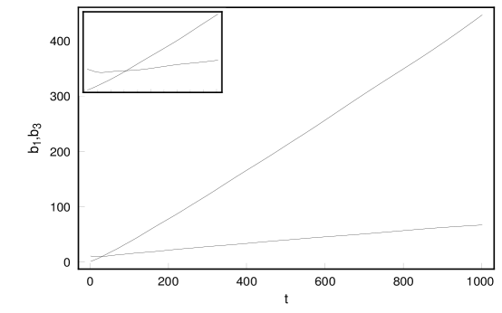
Figure 1: The behavior of metric variables for initial conditions $b_{1}=0.50,b_{3}=11.12,P_{3}=0.03,\alpha=\gamma=0.1,P_{\alpha}=-0.67,P_{\gamma}=0.03$. The inserted figure covers $0\leq t\leq 100$ and indicates an initial decrease in $b_{3}$ which quickly reverses direction.

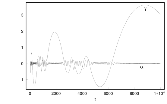
Figure 2: The behavior of YM field variables in axially symmetric Bianchi I-EYM cosmology for the initial conditions $b_{1}=2,b_{3}=1,P_{3}=\alpha=\gamma=P_{\alpha}=0.1,P_{\gamma}=0.2$. The oscillations of $\gamma$ are characterized by higher amplitudes and lower frequencies.

In fact, we used a fifth order Runge-Kutta integrator to integrate the system (36) and computed the Hamiltonian constraint to check the accuracy of the numerical integration.

As figure 2 and the YM equations indicate, the general behavior of the YM fields is that of two coupled anharmonic oscillators with time-dependent frequencies. The behavior of the YM field variables in the above system resembles the dynamical properties of homogeneous YM fields in flat space known as Yang-Mills Classical Mechanics (YMCM) [19].

4 Axially symmetric YM fields in flat space and regularizing effects of gravitational self-interaction

A full analysis of the dynamical system (36) is an insurmountable task. Therefore we decided to start our analysis from the simpler system of axially symmetric YM fields in flat space. Fortunately, the procedure described in section 2 encompasses the gauge fixing for homogeneous YM fields in flat space. It is well known that YMCM has stochastic properties [19],[23],[6],[14]. In these models the reduction from the full space of dynamical variables to lower dimensions to make the dynamical evolution tractable is via some ansatz. In our model, the reduction is an inevitable consequence of the space-time symmetry.

The two dimensional flat system $\Lambda^{1}_{1}\not=0,\Lambda^{2}_{2}\not=0$ and the three dimensional flat system $\Lambda^{1}_{1}\not=0,\Lambda^{2}_{2}\not=0,\Lambda^{3}_{3}\not=0$, all other components vanishing, have been extensively covered in [23] and [6]. The stochastic character of these systems is demonstrated by numerically computing the Liapunov index. Such numerical computations are achieved by the simultaneous integration of the first order system $\dot{\mathbf{x}}=\mathbf{V}(\mathbf{x})$ and the linearized first order system $\dot{\mathbf{w}}=M(\mathbf{x}).\mathbf{w}$ in which $\mathbf{w}$ is the perturbation vector connecting two nearby trajectories and $M(\mathbf{x})$ is the Jacobian matrix of $\mathbf{V}(x)$ [18]. The Liapunov exponent is defined as

$$\sigma=\lim_{t\rightarrow\infty}\frac{1}{t}\ln{\frac{|\mathbf{w}(t)|}{|\mathbf{w}(0)|}}.$$ (39)

We follow the procedure explained in [7] to compute the Liapunov index for axially symmetric YM fields first in flat space and later in a Bianchi I cosmology.

The dynamics of axially symmetric YM fields in flat space is governed by the system

$$\ddot{\alpha}+\alpha(\gamma^{2}+\alpha^{2}) = 0,$$ (40)

$$\ddot{\gamma}+2\alpha^{2}\gamma = 0,$$ (41)

which correspond to a set of two strongly coupled oscillators with varying frequencies and amplitudes. These equations are derived from the Hamiltonian

$$H=\frac{1}{2}(\dot{\gamma}^{2}+2\dot{\alpha}^{2}+2\alpha^{2}\gamma^{2}+\alpha^{4}).$$ (42)

The system describes the motion of a point particle moving in a potential well $U=\alpha^{2}\gamma^{2}+\alpha^{4}/2$ with two open channels in the directions of positive and negative $\gamma$ (figure 3). In these channels the term quartic in $\alpha$ in U is much smaller than the term quadratic in $\alpha$. Therefore the behavior of the point particle in each channel is basically the same as that of the point particle in the two dimensional Hamiltonian system

$$H=\frac{1}{2}(\dot{\alpha}^{2}\dot{\gamma}^{2}+\alpha^{2}\gamma^{2})$$ (43)

treated in [19]. The potential barrier in this system has open channels both in $\alpha$ and $\gamma$ directions and such systems have been extensively studied because of their relation to the plasma confinement problems. Unless $\alpha\equiv 0$ or $\gamma\equiv 0$, as the particle moves deeper and deeper into the $\gamma$ channel, say, the frequency of oscillations in $\alpha$ increases while the amplitude decreases. However, at a finite value of $\gamma$, $\dot{\gamma}=0$ at which point the particle returns to the $\alpha\sim\gamma$ region. In this system, stochastic regions occupy a significant portion of the phase space and the regular region is limited to a very small ($\sim 0.005\%$) region of the phase space [8].

Figure 3: The behavior of a particle in potential well $U=\alpha^{2}\gamma^{2}+\alpha^{4}/2$.

The behavior of a particle in a system with potential barrier $U$ is basically the same. However, because of the lack of the existing channels in directions $\alpha$, oscillations of $\gamma$ are characterized by larger amplitudes and smaller frequencies.

Following [7] we numerically computed the Liapunov index for the system (40) and (41) for randomly selected initial conditions satisfying (42) with $H=1$. It turns out that the Liapunov index for this system is positive and is of the same order of magnitude as the one for the system (43)(see figure 4). Numerical investigations for randomly selected initial conditions indicate that in this system, stochastic regions occupy a large portion of the phase space also.

Figure 4: $\ln$ of the Liapunov exponent vs. $\ln$ of the evolution parameter for axially symmetric YM fields in flat space and in Bianchi I-EYM cosmology for initial conditions as in figure 2. This was a typical behavior for randomly selected initial conditions. (s) and (c) refer to synchronous and conformal time respectively.

There are at least two problems associated with generalizing the study of the stochastic properties of the flat space model to axially symmetric Bianchi I-EYM model represented by the system (36). One is related to the strongly coupled nature of the ODE system and the higher number of degrees of freedom which are known to cause sophisticated stochastic phase space properties like Arnold diffusion [18]. Numerical investigations (see figure 1) point to a non-compact phase space. Thus we can say that axially symmetric Bianchi I-EYM systems are not globally ergodic. However, we do not rule out the existence of ergodic components.

The other problem is related to the inherent gauge dependence in the definition of Liapunov exponent and the non-existence of a satisfactory gauge covariant definition of chaos in general relativity. It is known that in Mixmaster models the positivity of Liapunov exponents depends on the choice of time reparametrization [4]. However, in Mixmaster cosmology, the stochasticity is associated with the behavior of the metric variables in the vicinity of the cosmological singularity where cosmological time is not well defined. In Bianchi I-EYM any ergodicity, if there is any, is mainly in YM field variables, far away from the cosmological singularity.

Similar to the flat space scenario, we calculated the Liapunov exponents in both synchronous and conformal time of Bianchi I-EYM system for randomly selected initial values (see figure 4). The vanishing of Liapunov exponents in synchronous time point to a dynamical system in which the stochastic regions, if there are any, occupy a much smaller portion of the phase space. However , it also underlines the known fact that the Liapunov exponent is sensitive to time reparametrization. The Liapunov exponent is non-vanishing in conformal time with a value smaller than the corresponding flat space model. At this point we would like to add that it is more difficult to preserve the constraint in the conformal time and the numerical stability of the dynamical system is substantially enhanced in the synchronous time.

Following [5] we computed the correlation between the initial and final values of YM field variables as an indication of a particular statistical independence in the dynamical evolution of the field variables. As figure 5 demonstrates, after a large time evolution, there is a loss of correlation between $\gamma_{i}$ and $\gamma_{f}$ (respectively $\alpha_{i}$ and $\alpha_{f}$). Therefore $\gamma_{i}(\alpha_{i})$ and $\gamma_{f}(\alpha_{f})$ can be regarded as two stochastically independent random variables.

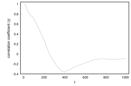
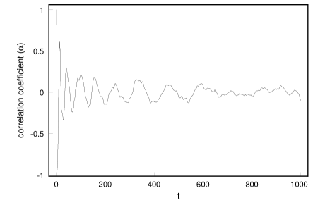
Figure 5: The correlation between $\gamma_{f}$ and $\gamma_{i}$ in terms of time for the initial conditions $b_{1}=b_{3}=1,P_{1}=2,P_{3}=1,P_{\alpha}=-.28$. In the left figure $\alpha=0.1,0.15\leq\gamma\leq 17.25$ and in the right figure $\gamma=0.1,0.15\leq\alpha\leq 1.56$. The large time behavior indicates that there is no clear correlation between $\gamma_{f}(\alpha_{f})$ and $\gamma_{i}(\alpha_{i})$.

5 Conclusion

We systematically derived the most general form of the YM connection and the EYM field equations in Bianchi cosmologies with a four-dimensional isometry group in which the Killing vector fields obey the commutation relations (4). For the simplest of Bianchi cosmologies, namely Bianchi I, we investigated the resulting dynamical system. In doing so, one realizes that there is little hope to find an exact solution. Numerical integration suggests a non-compact phase space and oscillatory behavior for the YM field variables. However, one can easily use the above mentioned scheme to construct invariant YM connections in flat space. There has been extensive work on the dynamical properties of homogeneous YM fields in flat space (YMCM) which are known to have stochastic properties. We used some methods to investigate chaos in YMCM (i.e numerical computation of Liapunov exponent) to see how gravitational self-interaction can affect the stochastic behavior. It turned out that the system with gravitational self-interaction has milder stochastic properties. We hope to extend this work to other Bianchi cosmologies.

References

- [1] R. Bartnik, The spherically symmetric Einstein Yang-Mills equations, Relativity Today (Z. Perjés, ed.), Nova Science Pub., Commack NY, 1992, pp. 221–240.
- [2] J. Beckers, J. Harnard, M. Perround, and P. Winternitz, Tensor fields invariant under subgroups of the conformal group of space-time, J. Math. Phys. 19 (1978), 1978, 2126–2153.
- [3] O. Brodbeck and N. Straumann, A generalized Birkhoff theorem for the Einstein-Yang-Mills system, J. Math. Phys. 34 (1993), 1993, 2412–2423.
- [4] A. Burd, How can you tell if the Bianchi IX models are chaotic?, Deterministic chaos in general relativity (D. Hobill, ed.), 1993, Kananaskis, Plenum Press, New York, 1994, pp. 345–354.
- [5] E. Calzetta and C. El Hasi, Chaotic Friedman-Robertson-Walker cosmology, Classical Quantum Gravity 10 (1993), 1993, 1825–1841.
- [6] B.V. Chirikov and D.L. Shepelyanskiĭ, Stochastic oscillations of classical Yang-Mills fields, JETP Lett. 34 (1981), 1981, 163–166.
- [7] B.V. Chirikov and D.L. Shepelyanskiĭ, Dynamics of some homogeneous models of classical Yang-Mills fields, Soviet J. Nuclear Phys. 36 (1982), 1982, 908–915.
- [8] P. Dahlqvist and G. Russberg, Existence of stable orbits in potential, Phys. Rev. Lett. 65 (1990), 1990, 2837–2838.
- [9] L.H. Ford, Inflation driven by a vector field, Phys. Rev. D (3) 40 (1989), 1989, 967–972.
- [10] D.V. Gal’tsov and M.S. Volkov, Yang-Mills cosmology. cold matter for a hot universe, Phys. Lett. B 256 (1991), 1991, 17–21.
- [11] G.W. Gibbons and A.R. Steif, Yang-Mills cosmologies and collapsing gravitational sphalerons, Phys. Lett. B 320 (1994), 1994, 245–252.
- [12] J. Harnad, S. Shnider, and L. Vinet, Group actions on principal bundles and invariance conditions for gauge fields, J. Math. Phys. 21 (1980), 1980, 2719–2724.
- [13] Y. Hosotani, Exact solution to the Einstein-Yang-Mills equations, Phys. Lett. B 147 (1984), 1984, 44–46.
- [14] J. Karkowski, Chaos in Yang-Mills mechanics, Acta Phys. Polon. B 21 (1990), 1990, 529–540.
- [15] S. Kobayashi and K. Nomizu, Foundations of differential geometry II, Interscience Wiley New York, 1969.
- [16] D. Kramer, H. Stephani, M. MacCallum, and E. Herlt, Exact solutions of Einstein’s field equations, VEB Deutscher Verlag der Wissenschaften, 1980.
- [17] H.P. Künzle, -Einstein-Yang-Mills fields with spherical symmetry, Classical Quantum Gravity 8 (1991), 1991, 2283–2297.
- [18] A.J. Lichtenberg and M.A. Lieberman, Regular and chaotic dynamics (2nd ed.), Springer-Verlag, 1990.
- [19] S.G. Matinyan, G.K. Savvidi, and N.G. Ter-Arutyunyan-Savvidi, Classical Yang-Mills mechanics. nonlinear color oscillations, Soviet Phys. JETP 53 (1981), 1981, 421–425.
- [20] P.V. Moniz and J.M. Mourão, Homogeneous and isotropic closed cosmologies with a gauge sector, Classical Quantum Gravity 8 (1991), 1991, 1815–1831.
- [21] G. Rosen, Spatially homogeneous solutions to the Einstein-Maxwell equations, Phys. Rev. B (3) 136 (1964), 1964, 297–298.
- [22] M.P. Ryan and L.C. Shepley, Homogeneous relativistic cosmologies, Princeton University Press, 1975.
- [23] G.K. Savvidy, The Yang-Mills classical mechanics as a Kolmogorov -system, Phys. Lett. B 130 (1983), 1983, 303–307.
- [24] J.M. Stewart and G.F.R. Ellis, Solutions of Einstein’s equations for a fluid which exhibit local rotational symmetry, J. Math. Phys. 9 (1968), 1968, 1072–1082.
- [25] K.S. Thorne, Primordial element formation, primordial magnetic fields, and the isotropy of the universe, Astrophys. J. 148 (1967), 1967, 151.
- [26] Y. Verbin and A. Davidson, Quantized non-Abelian wormholes, Phys. Lett. B 229 (bh), bh, 364–367.