Abstract

Quantum inequality restrictions on the stress-energy tensor for negative energy are developed for three and four-dimensional static spacetimes. We derive a general inequality in terms of a sum of mode functions which constrains the magnitude and duration of negative energy seen by an observer at rest in a static spacetime. This inequality is evaluated explicitly for a minimally coupled scalar field in three and four-dimensional static Robertson-Walker universes. In the limit of vanishing curvature, the flat spacetime inequalities are recovered. More generally, these inequalities contain the effects of spacetime curvature. In the limit of short sampling times, they take the flat space form plus subdominant curvature-dependent corrections.

1 Introduction

Recently, several approaches have been proposed to study the extent to which quantum fields may violate the “weak energy condition,” (WEC) $T_{\mu\nu}u^{\mu}u^{\nu}\geq 0$, for all timelike vectors $u^{\mu}$. Such violations occur in the Casimir effect and in quantum coherence effects, where the energy density in a region may be negative. Violations of the local energy conditions first led to the averaging of the energy condition over timelike (or null) geodesics[1]. This eventually led to the “averaged weak energy condition”,

$$\int_{-\infty}^{\infty}T_{\mu\nu}u^{\mu}u^{\nu}d\tau\geq 0.$$ (1)

Here the total energy density averaged along an entire geodesic is constrained to be positive. While this does preserve in some form the weak energy condition, it does not constrain the magnitude of the negative energy violations from becoming arbitrarily large over an arbitrary interval, so long as there is compensating positive energy elsewhere. In cases such as the Casimir effect, where there is a constant negative energy density present in the vacuum state, Eq. (1) fails. However, it is often still possible to prove “difference inequalities” in which $T_{\mu\nu}$ is replaced by the difference in expectation values between an arbitrary state and the vacuum state [2, 3].

Quantum inequality (QI) type relations have been proven [2, 4, 5] which do constrain the magnitude and extent of negative energy. For example, in 4D Minkowski space the quantum inequality for free, quantized, massless scalar fields can be written in its covariant form as

$$\hat{\rho}={\tau_{0}\over\pi}\int_{-\infty}^{\infty}{\langle T_{\mu\nu}u^{\mu}u^{\nu}\rangle d\tau\over{\tau^{2}+\tau_{0}^{2}}}\geq-{3\over 32\pi^{2}\tau_{0}^{4}},$$ (2)

for all values of $\tau_{0}$ and where $u^{\mu}$ is a timelike vector. The expectation value $\langle\rangle$ is with respect to an arbitrary state $|\psi\rangle$, and $\tau_{0}$ is the characteristic width of the sampling function, $\tau_{0}/\pi(\tau^{2}+\tau_{0}^{2})$, whose time integral is unity. Such inequalities limit the magnitude of the negative energy violations and the time for which they are allowed to exist. In addition, such QI relations reduce to the usual AWEC type conditions in the infinite sampling time limit.

Flat space quantum inequality-type relations of this form have since been applied to curved spacetimes [6, 7] by keeping the sampling time shorter than a “characteristic” curvature radius of the geometry. Under such circumstances, it was argued that the spacetime is approximately flat, and the inequalities could be applied over a small region. In the wormhole geometry [6], this led to wormholes which were either on the order of a Planck length in size or with a great disparity in the length scales that characterize the wormhole. In the “warp drive” geometry [8] it was found that if one wanted superluminal bubbles of macroscopically useful size then the bubble wall thickness would be of the order of a Planck length [7]. Although the method of small sampling times is useful, it does not address the question of how the curvature would enter into the quantum inequalities for arbitrarily long sampling times.

In this paper we will address this issue. We will begin with a generalized theory in Section 2 which will allow us to find quantum difference inequalities in a globally static, but arbitrarily curved spacetime Then in Section 3 we will look at the case of the $S^{2}\times R$ spacetime, the 3D equivalent to the Einstein universe. We will show that the QI’s are modified by a “scale function” which is dependent upon the ratio of sampling time to the curvature radius ($t_{0}/a$). In Section 4, we will proceed to find similar QI’s for the three cases of the 4D static Robertson-Walker spacetimes. In conclusion, we will discuss how AWEC type conditions in these particular spacetimes can be found. We will use units in which $\hbar=c=G=1$.

2 General Theory

In this section, we will develop a formalism to find the quantum inequalities for a massive, minimally coupled scalar field in a generalized spacetime. This method will be applicable in globally static spacetimes, allowing us to use a separation of variables of the wave equation, and write the positive frequency mode functions as

$$f_{\lambda}({\bf x},t)=U_{\lambda}({\bf x})e^{-i\omega t}.$$ (3)

The label $\lambda$ represents the set of quantum numbers necessary to specify the state. Additionally, the mode functions should have unit Klein-Gordon norm

$$\left(f_{\lambda},f_{\lambda^{\prime}}\right)=\delta_{\lambda\lambda^{\prime}}.$$ (4)

The above separation of variables can be accomplished when $\partial_{t}$ is a timelike Killing vector. Such a spacetime can be described by a metric of the form

$${ds}^{2}=-{dt}^{2}+g_{ij}({\bf x})dx_{i}dx_{j}.$$ (5)

Here $g_{ij}$ is the metric of the spacelike hypersurfaces that are orthogonal to the Killing vector in the time direction. With this metric, the wave equation is

$$\mathord{\hbox{\bxfnt\char 116\relax}\hbox to0.0pt{\hss\bxfnt\char 117\relax}}\phi-\mu^{2}\phi=-\partial_{t}^{2}\phi+{1\over\sqrt{|g|}}\left(\partial_{i}\sqrt{|g|}g^{ij}\partial_{j}\phi\right)-\mu^{2}\phi=0,$$ (6)

where $g={\rm det}(g_{\mu\nu})$. The scalar field $\phi$ can then be expanded in terms of creation and annihilation operators as

$$\phi=\sum_{\lambda}{\bigl{(}a_{\lambda}f_{\lambda}+a^{\dagger}_{\lambda}f^{\ast}_{\lambda}\bigr{)}},$$ (7)

when quantization is carried out over a finite box or universe. If the spacetime is itself infinite, then we replace the summation by an integral over all of the possible modes. The creation and annihilation operators satisfy the usual commutation relations [9].

In principle, quantum inequalities can be found for any geodesic observer [2]. In the Robertson-Walker universes, static observers see the universe as having maximal symmetry. Moving observers lose this symmetry, and in general the mode functions of the wave equation can become quite complicated. Thus, for this paper we will concern ourselves only with static observers, whose four-velocity is the timelike Killing vector. The energy density that such an observer samples is given by

$$\rho=T_{\mu\nu}u^{\mu}u^{\nu}=T_{00}={1\over 2}\left[(\partial_{t}\phi)^{2}+\partial^{j}\phi\partial_{j}\phi+\mu^{2}\phi^{2}\right]\,.$$ (8)

Upon substitution of the above mode function expansion into Eq. (8), one finds

$$T_{00} = {\rm Re}\sum_{\lambda\lambda^{\prime}}\left\{{\omega\omega^{\prime}}\left[U_{\lambda}^{*}U_{\lambda^{\prime}}e^{+i(\omega-\omega^{\prime})t}a_{\lambda}^{\dagger}a_{\lambda^{\prime}}-U_{\lambda}U_{\lambda^{\prime}}e^{-i(\omega+\omega^{\prime})t}a_{\lambda}a_{\lambda^{\prime}}\right]\right.$$ (9)

$$\qquad+\left[\partial^{j}U_{\lambda}^{*}\partial_{j}U_{\lambda^{\prime}}e^{+i(\omega-\omega^{\prime})t}a_{\lambda}^{\dagger}a_{\lambda^{\prime}}+\partial^{j}U_{\lambda}\partial_{j}U_{\lambda^{\prime}}e^{-i(\omega+\omega^{\prime})t}a_{\lambda}a_{\lambda^{\prime}}\right]$$

$$\qquad+\mu^{2}\left.\left[U_{\lambda}^{*}U_{\lambda^{\prime}}e^{+i(\omega-\omega^{\prime})t}a_{\lambda}^{\dagger}a_{\lambda^{\prime}}+U_{\lambda}U_{\lambda^{\prime}}e^{-i(\omega+\omega^{\prime})t}a_{\lambda}a_{\lambda^{\prime}}\right]\right\}$$

$$+{1\over 2}\sum_{\lambda}\left(\omega^{2}U_{\lambda}^{*}U_{\lambda}+\partial^{j}U_{\lambda}^{*}\partial_{j}U_{\lambda}+\mu^{2}U_{\lambda}^{*}U_{\lambda}\right)$$

The last term is the expectation value in the vacuum state, defined by $a_{\lambda}|0\rangle=0$ for all $\lambda$, and is formally divergent. The vacuum energy density may be defined by a suitable regularization and renormalization procedure, as will be discussed in more detail in Section 3 and 4. In general, however, it is not uniquely defined. This ambiguity may be side-stepped by concentrating attention upon the difference between the energy density in an arbitrary state and that in the vacuum state, as was done in Ref. [2]. We will therefore concern ourselves primarily with

$$:T_{00}:\;=T_{00}-\langle 0|T_{00}|0\rangle,$$ (10)

where $|0\rangle$ represents the Fock vacuum state defined by the global timelike Killing vector. We will average the energy density as in Eq. (2), and find that the averaged energy density difference is given by

$$\Delta\hat{\rho} \equiv {t_{0}\over\pi}\int_{-\infty}^{\infty}{{\langle:T_{00}:\rangle dt}\over{t^{2}+t_{0}^{2}}}$$ (11)

$$= {\rm Re}\sum_{\lambda\lambda^{\prime}}\left\{{\omega\omega^{\prime}}\left[U_{\lambda}^{*}U_{\lambda^{\prime}}e^{-|\omega-\omega^{\prime}|t_{0}}\langle a_{\lambda}^{\dagger}a_{\lambda^{\prime}}\rangle-U_{\lambda}U_{\lambda^{\prime}}e^{-(\omega+\omega^{\prime})t_{0}}\langle a_{\lambda}a_{\lambda^{\prime}}\rangle\right]\right.$$

$$\qquad+\left[\partial^{j}U_{\lambda}^{*}\partial_{j}U_{\lambda^{\prime}}e^{-|\omega-\omega^{\prime}|t_{0}}\langle a_{\lambda}^{\dagger}a_{\lambda^{\prime}}\rangle+\partial^{j}U_{\lambda}\partial_{j}U_{\lambda^{\prime}}e^{-(\omega+\omega^{\prime})t_{0}}\langle a_{\lambda}a_{\lambda^{\prime}}\rangle\right]$$

$$\qquad+\mu^{2}\left.\left[U_{\lambda}^{*}U_{\lambda^{\prime}}e^{-|\omega-\omega^{\prime}|t_{0}}\langle a_{\lambda}^{\dagger}a_{\lambda^{\prime}}\rangle+U_{\lambda}U_{\lambda^{\prime}}e^{-(\omega+\omega^{\prime})t_{0}}\langle a_{\lambda}a_{\lambda^{\prime}}\rangle\right]\right\}$$

We are seeking a lower bound on this quantity. It has been shown [10] that

$${\rm Re}\sum_{\lambda\lambda^{\prime}}f(\lambda)^{*}f(\lambda^{\prime})e^{-|\omega-\omega^{\prime}|t_{0}}\langle a_{\lambda}^{\dagger}a_{\lambda^{\prime}}\rangle\geq{\rm Re}\sum_{\lambda\lambda^{\prime}}f(\lambda)^{*}f(\lambda^{\prime})e^{-(\omega+\omega^{\prime})t_{0}}\langle a_{\lambda}^{\dagger}a_{\lambda^{\prime}}\rangle.$$ (12)

Upon substitution of this into Eq. (11) we have

$$\Delta\hat{\rho} \geq {\rm Re}\sum_{\lambda\lambda^{\prime}}\left\{{\omega\omega^{\prime}}\left[U_{\lambda}^{*}U_{\lambda^{\prime}}\langle a_{\lambda}^{\dagger}a_{\lambda^{\prime}}\rangle-U_{\lambda}U_{\lambda^{\prime}}\langle a_{\lambda}a_{\lambda^{\prime}}\rangle\right]\right.$$ (13)

$$\qquad+\left[\partial^{j}U_{\lambda}^{*}\partial_{j}U_{\lambda^{\prime}}\langle a_{\lambda}^{\dagger}a_{\lambda^{\prime}}\rangle+\partial^{j}U_{\lambda}\partial_{j}U_{\lambda^{\prime}}\langle a_{\lambda}a_{\lambda^{\prime}}\rangle\right]$$

$$\qquad+\mu^{2}\left.\left[U_{\lambda}^{*}U_{\lambda^{\prime}}\langle a_{\lambda}^{\dagger}a_{\lambda^{\prime}}\rangle+U_{\lambda}U_{\lambda^{\prime}}\langle a_{\lambda}a_{\lambda^{\prime}}\rangle\right]\right\}e^{-(\omega+\omega^{\prime})t_{0}}\,.$$

We may now apply the inequalities proven in the Appendix. For the first and third term of Eq. (13), apply Eq. (A7) with $h_{\lambda}=\omega\,U_{\lambda}{\rm e}^{-\omega t_{0}}$ and $h_{\lambda}=\mu\,U_{\lambda}{\rm e}^{-\omega t_{0}}$, respectively. For the second term of Eq. (13), apply Eq. (A1) with $A_{ij}=g_{ij}$ and $h_{\lambda}^{i}=\partial^{i}U_{\lambda}{\rm e}^{-\omega t_{0}}$. The result is

$$\Delta\hat{\rho}\geq-{1\over 2}\sum_{\lambda}\left(\omega_{\lambda}^{2}U_{\lambda}^{*}U_{\lambda}+\partial^{j}U_{\lambda}^{*}\,\partial_{j}U_{\lambda}+\mu^{2}U_{\lambda}^{*}U_{\lambda}\right)e^{-2\omega_{\lambda}t_{0}}.$$ (14)

This inequality may be re-written using the equation satisfied by the spatial mode functions:

$$\nabla^{j}\nabla_{j}U_{\lambda}+(\omega^{2}-\mu^{2})U_{\lambda}=0\,,$$ (15)

to obtain

$$\Delta\hat{\rho}\geq-\sum_{\lambda}\left(\omega_{\lambda}^{2}+{1\over 4}\nabla^{j}\nabla_{j}\right)|U_{\lambda}|^{2}{\rm e}^{-2\omega_{\lambda}t_{0}}\,.$$ (16)

Here $\nabla^{i}$ is the covariant derivative operator in the $t={\rm constant}$ hypersurfaces. Therefore, given any metric which admits a global timelike Killing vector, we can calculate the limitations on the negative energy densities once the solutions to the wave equation in that curved background are known.

Note that although the local energy density may be more negative in a given quantum state than in the vacuum, the total energy difference integrated over all space is non-negative. This follows from the fact that the normal-ordered Hamiltonian,

$$:H:\;=\int:T_{00}:\,\sqrt{-g}\,d^{n}x=\sum_{\lambda}\omega_{\lambda}\,a_{\lambda}^{\dagger}a_{\lambda}\,,$$ (17)

is a positive-definite operator, so that $\langle:H:\rangle\geq 0$.

In the following sections, we will apply the general energy density inequality, Eq. (16), to three and four-dimensional Robertson-Walker universes.

3 Quantum Inequality in a 3D Closed Universe

Let us consider the three-dimensional spacetime with a length element given by

$$ds^{2}=-dt^{2}+a^{2}\left(d\theta^{2}+\sin^{2}\theta d\varphi^{2}\right)$$ (18)

Here constant time slices of this universe are two spheres of radius $a$. The wave equation on this background with a coupling of strength $\xi$ to the Ricci scalar $R$ is

$$\mathord{\hbox{\bxfnt\char 116\relax}\hbox to0.0pt{\hss\bxfnt\char 117\relax}}\phi-(\mu^{2}+\xi R)\phi=0.$$ (19)

For the metric Eq. (18), this equation becomes

$$-\partial_{t}^{2}\phi+{1\over{a^{2}\sin\theta}}\partial_{\theta}\left(\sin\theta\partial_{\theta}\phi\right)+{1\over{a^{2}\sin^{2}\theta}}\partial_{\varphi}^{2}\phi-[\mu^{2}+\xi\left(2\over a^{2}\right)]\phi=0,$$ (20)

which has the solutions

$$f_{lm}(t,\theta,\varphi)={1\over{\sqrt{2a^{2}\omega}}}{\rm Y}_{lm}(\theta,\varphi)e^{-i\omega_{l}t} l=0,1,2,\cdots$$ (21)

$$-l\leq m\leq l,$$ (22)

with eigenfrequencies

$$\omega_{l}=a^{-1}\sqrt{l(l+1)+2\xi+\mu^{2}a^{2}}\,.$$ (23)

The ${\rm Y}_{lm}$ are the usual spherical harmonics with unit normalization. The coupling parameter $\xi$ here can be seen to contribute to the wave functions as a term of the same form as the mass. In this paper, however, we will look only at minimal coupling ($\xi=0$). The lower bound on the energy density is then given by

$$\Delta\hat{\rho}\geq-{1\over{2a^{2}}}\sum_{l=0}^{\infty}\sum_{m=-l}^{+l}\omega_{l}|{\rm Y}_{lm}(\theta,\varphi)|^{2}e^{-2\omega_{l}t_{0}}-{1\over 8a^{2}}\nabla^{i}\nabla_{i}\sum_{l=0}^{\infty}\sum_{m=-l}^{+l}{1\over\omega_{l}}|{\rm Y}_{lm}(\theta,\varphi)|^{2}e^{-2\omega_{l}t_{0}}$$ (24)

However the spherical harmonics obey a sum rule [11]

$$\sum_{m=-l}^{+l}|{\rm Y}_{lm}(\theta,\varphi)|^{2}={{2l+1}\over{4\pi}}.$$ (25)

We immediately see that the difference inequality is independent of position, as expected from the spatial homogeneity, and that the second term of Eq. (24) does not contribute. We have

$$\Delta\hat{\rho}\geq-{1\over{8\pi a^{2}}}\sum_{l=0}^{\infty}(2l+1)\,\omega_{l}e^{-2\omega_{l}t_{0}}.$$ (26)

This summation is finite due to the exponentially decaying term. We are now left with evaluating the sum for a particular set of values for the mass $\mu$, the radius $a$, and the sampling time $t_{0}$. Let $\eta={t_{0}/a}$. Then

$$\Delta\hat{\rho}\geq-{1\over{16\pi t_{0}^{3}}}\left[2\eta^{3}\sum_{l=1}^{\infty}(2l+1)\,\tilde{\omega}_{l}\,{\rm e}^{-2\eta\tilde{\omega}_{l}}\right]=-{1\over{16\pi t_{0}^{3}}}F(\eta,\mu)$$ (27)

where

$$\tilde{\omega}_{l}=\sqrt{l(l+1)+a^{2}\mu^{2}}$$ (28)

The coefficient $-{1/(16\pi t_{0}^{3})}$ is the right hand side of the inequality for the case of a massless field in an infinite 3-D Minkowski space. The “scale function”, $F(\eta,\mu)$, represents how the mass and the curvature of the closed spacetime affects the difference inequality.

3.1 Massless Case

In terms of the variable $\eta={t_{0}/a}$, which is the ratio of the sampling time to the radius of the universe, we can write the above expression for $F(\eta,0)$ as

$$F(\eta)=F(\eta,0)=2\eta^{3}\sum_{l=1}^{\infty}(2l+1)\sqrt{l(l+1)}\,{\rm e}^{-2\eta\sqrt{l(l+1)}}$$ (29)

A plot of $F(\eta)$ is shown in Figure 1. In the limit of $\eta\rightarrow 0$, when the sampling time is very small or the radius of the universe has become so large that it approximates flat space, then the function $F(\eta)$ approaches 1, yielding the flat space inequality. .

We can look at the inequality in the two asymptotic regimes of $\eta$. In the large $\eta$ regime each term of greater $l$ in the exponent will decay away faster than the previous. The $l=1$ term yields a good approximation. In the other regime, when the sampling time is small compared to the radius, we can use the Plana summation formula to calculate the summation explicitly:

$$\sum_{n=1}^{\infty}f(n)+{1\over 2}f(0)=\int_{0}^{\infty}f(x)dx+i\int_{0}^{\infty}{f(ix)-f(-ix)\over{{\rm e}^{2\pi x}-1}}dx\,,$$ (30)

where

$$f(x)=(2x+1)\sqrt{x(x+1)}\,{\rm e}^{-2\eta\sqrt{x(x+1)}}.$$ (31)

Immediately we see that for our summation $f(0)=0$. The first integral can be done with relative ease yielding

$$\int_{0}^{\infty}f(x)dx=\int_{0}^{\infty}(2x+1)\sqrt{x(x+1)}\,{\rm e}^{-2\eta\sqrt{x(x+1)}}dx=\frac{1}{2\eta^{3}}\,.$$ (32)

This term reproduces the flat space inequality. The second integral in Eq. (30) therefore contains all the corrections due to non-zero curvature of the spacetime. Since $\eta$ is small, we can Taylor expand the exponent around $\eta=0$, and then keep the lowest order terms. One finds

$$i\int_{0}^{\infty}{f(ix)-f(-ix)\over{e^{2\pi x}-1}}dx\sim-I_{0}-\eta I_{1}+\cdots\,,$$ (33)

where

$$I_{0}=\int_{0}^{\infty}\sqrt{2x}\;{\left(2x\sqrt{\sqrt{x^{2}+1}-x}+\sqrt{\sqrt{x^{2}+1}+x}\right)\over{{\rm e}^{2\pi x}-1}}\;dx\approx 0.265096$$ (34)

and

$$I_{1}=\int_{0}^{\infty}{4x(2x^{2}-1)\over{{\rm e}^{2\pi x}-1}}dx=-\frac{2}{15}\,.$$ (35)

Therefore the function $F(\eta)$ in the small $\eta$ limit is given by

$$F(\eta)\simeq 1-0.530192\,\eta^{3}+{4\over 15}\eta^{4}+O(\eta^{5})+\cdots$$ (36)

and in the large $\eta$ limit by

$$F(\eta)\simeq 6\sqrt{2}\,\eta^{3}\,{\rm e}^{-2\sqrt{2}\eta}+\cdots\,.$$ (37)

Both of these asymptotic forms are plotted along with the exact form of $F(\eta)$ in Figure 1. The graph shows that the two asymptotic limits follow the exact graph to a very large precision except in the interval of $1<\eta<2$. These results for the function $F(\eta)$, combined with Eq. (27), yield the difference inequality for the massless scalar field.

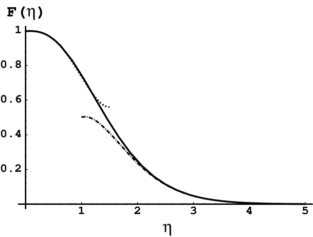
Figure 1:

Plot of the Scale Function $F(\eta)$ and its asymptotic forms. The solid line is the exact form of the function. The dotted line is the small $\eta$ approximation, while the dot-dash line is the large $\eta$ approximation.

The difference inequality does not require knowledge of the actual value of the renormalized vacuum energy, $\rho_{0}$. However, if we wish to obtain a bound on the energy density itself, we must combine the difference inequality and $\rho_{0}$. One procedure for computing $\rho_{0}$ is analogous to that used to find the Casimir energy in flat spacetime with boundaries: one defines a regularized energy density, subtracts the the corresponding flat space energy density, and then takes the limit in which the regulator is removed. A possible choice of regulator is to insert a cutoff function, $g(\omega)$, in the mode sum and define the regularized energy density as

$$\rho_{reg}=\frac{1}{8\pi a^{2}}\sum_{\lambda}\omega_{\lambda}\,g(\omega_{\lambda})=\frac{1}{8\pi a^{2}}\sum_{l=0}^{\infty}(2l+1)\,\omega_{l}\,g(\omega_{l})\,.$$ (38)

In the limit that $a\rightarrow\infty$, we may replace the sum by an integral and obtain the regularized flat space energy density:

$$\rho_{FSreg}=\frac{1}{4\pi}\int_{0}^{\infty}{\rm d}\omega\,\omega\,g(\omega)\,.$$ (39)

The renormalized vacuum energy density may then be defined as

$$\rho_{0}=\lim_{g\rightarrow 1}(\rho_{reg}-\rho_{FSreg})\,.$$ (40)

The vacuum energy density so obtained will be denoted by $\rho_{Casimir}$. An analogous procedure was used in Ref. [12] to obtain the vacuum energy density for the conformal scalar field in the 4D Einstein universe. An explicit calculation for the present case, again using the Plana summation formula, yields

$$\rho_{Casimir}=-{I_{0}\over{8\pi a^{3}}}\approx-{0.265096\over{8\pi a^{3}}}.$$ (41)

This agrees with the result obtained by Elizalde [13] using the zeta function technique. In this case $\rho_{Casimir}<0$, whereas the analogous calculation for the conformal scalar field in this three-dimensional spacetime yields a positive vacuum energy density, $\rho_{Casimir}=1/{96\pi a^{3}}$. It should be noted that this procedure works in this case only because the divergent part of $\rho_{reg}$ is independent of $a$. More generally, there may be curvature-dependent divergences which must also be removed.

Let us now return to the explicit forms of the difference inequality. In the limit that $t_{0}\gg a$, Eqs. (27) and (37) yield

$$\Delta\hat{\rho}\geq-{{3\sqrt{2}}\over{8\pi a^{3}}}\,{\rm e}^{-2\sqrt{2}\,t_{0}/a}\,.$$ (42)

Similarly, in the limit that $t_{0}\ll a$, we find

$$\Delta\hat{\rho}\geq-{1\over{16\pi t_{0}^{3}}}-\rho_{Casimir}-{{t_{0}}\over{60\pi a^{4}}}+\cdots\,.$$ (43)

Thus the bound on the renormalized energy density in an arbitrary quantum state in the latter limit becomes

$$\hat{\rho}_{ren}\geq-{1\over{16\pi t_{0}^{3}}}-{{t_{0}}\over{60\pi a^{4}}}+\cdots\,.$$ (44)

From either of Eqs. (43) or (44) in the $a\rightarrow\infty$ limit we obtain the flat space limit. Here $\rho_{0}=0$ so $\Delta\rho=\rho$. In 3D flat space we can write the quantum inequality in a more covariant form as

$$\hat{\rho}={\tau_{0}\over\pi}\int_{-\infty}^{\infty}{\langle T_{\mu\nu}u^{\mu}u^{\nu}\rangle d\tau\over{\tau^{2}+\tau_{0}^{2}}}\geq-{1\over 16\pi\tau_{0}^{3}},$$ (45)

In the other limit when the sampling time becomes long, we find that $\Delta\hat{\rho}$ decays exponentially as a function of the sampling time. This simply reflects the fact that the difference in energy density between an arbitrary state and the vacuum state satisfies the averaged weak energy condition, Eq. (1).

4 4D Robertson-Walker Universes

Now we will apply the same method to the case of the three homogeneous and isotropic universes given by the four-dimensional static Robertson-Walker metrics. Here we have

$$[\epsilon=0]:\qquad g_{ij}dx^{i}dx^{j}=dx^{2}+dy^{2}+dz^{2}$$ (46)

for the flat universe with no curvature (Minkowski spacetime). For the closed universe with constant radius $a$, i.e. the universe of constant positive curvature, the spatial length element is given by.

$$[\epsilon=1]:\qquad g_{ij}dx^{i}dx^{j}=a^{2}\left[d\chi^{2}+\sin^{2}\chi(d\theta^{2}+\sin^{2}\theta d\varphi^{2})\right]\,,$$ (47)

where $0\leq\chi<\pi$, $0\leq\theta<\pi$, and $0\leq\varphi<2\pi$. The open universe $[\epsilon=-1]$ is given by making the replacement $\sin\chi\rightarrow\sinh\chi$ in Eq. (47) and now allowing $\chi$ to take on the values $0\leq\chi<\infty$. To find the lower bound of the quantum inequalities above we must solve for the eigenfunctions of the covariant Helmholtz equation

$$\nabla_{i}\nabla^{i}U_{\lambda}({\bf x})+(\omega^{2}_{\lambda}-\mu^{2})U_{\lambda}({\bf x})=0$$ (48)

where $\mu$ is the mass of the scalar field and $\omega_{\lambda}$ is the energy. A useful form of the solutions for this case is given by Parker and Fulling [14].

4.1 Flat and Open Universes in 4D

One finds that in the notation developed in Section 2, the spatial portion of the wave functions for flat (Euclidean) space is given by (continuum normalization)

$$[\epsilon=0]: U_{\bf k}({\bf x})=[2\omega(2\pi)^{3}]^{-1/2}e^{i{\bf k}\cdot{\bf x}},$$ (49)

$$\omega=\sqrt{|\bf k|^{2}+\mu^{2}}$$

$${\bf k}=(k_{1},k_{2},k_{3})\qquad(-\infty<k_{j}<\infty).$$

It is evident that $|U_{\bf k}|^{2}$ will be independent of position. This immediately removes the second term of the inequality in Eq. (16).

In the open universe the spatial functions are given by

$$[\epsilon=-1]: U_{\lambda}({\bf x})=(2a^{3}\omega_{q})^{-1/2}\Pi^{(-)}_{ql}(\chi){\rm Y}_{lm}(\theta,\varphi),$$ (51)

$$\omega_{q}=\sqrt{{(q^{2}+1)\over a^{2}}+\mu^{2}},$$

$$\lambda=(q,l,m).$$

Here, $0<q<\infty;\quad l=0,1,\cdots;$ and $m=-l,-l+1,\cdots,+l$. The sum over all states involves an integral over the radial momentum $q$. The functions $\Pi^{(-)}_{ql}(\chi)$ are given in Equation 5.23 of Birrell and Davies[9]. Apart from the normalization factor, they are

$$\Pi^{(-)}_{ql}(\chi)\propto\sinh^{l}\chi\left(d\over d\cosh\chi\right)^{l+1}\cos q\chi.$$ (53)

As with the mode functions of the 3-dimensional closed spacetime above, the mode functions of the open 4-dimensional universe satisfy an addition theorem [14, 15, 16]

$$\sum_{lm}|\Pi^{(-)}_{ql}(\chi){\rm Y}_{lm}(\theta,\varphi)|^{2}={q^{2}\over 2\pi^{2}}.$$ (54)

Since the addition theorem removes any spatial dependence, we again get no contribution from the Laplacian term of the quantum inequality, Eq. (16). Upon substitution of the mode functions for both the flat and open universes into the quantum inequality and using the addition theorem in the open spacetime case we have

$$[\epsilon=0]:\qquad\Delta\hat{\rho}\geq-{1\over 16\pi^{3}}\int_{-\infty}^{\infty}d^{3}k\,\omega_{\bf k}\,{\rm e}^{-2\omega_{\bf k}t_{0}}$$ (55)

and

$$[\epsilon=-1]:\qquad\Delta\hat{\rho}\geq-{1\over 4\pi^{2}a^{3}}\int_{0}^{\infty}dq\,q^{2}\,\omega_{q}\,{\rm e}^{-2\omega_{q}t_{0}},$$ (56)

respectively. The 3-dimensional integral in momentum space can be carried out by making a change to spherical momentum coordinates. The two cases can be written compactly as

$$\Delta\hat{\rho}\geq-{1\over 4\pi^{2}}\int_{0}^{\infty}dk\,k^{2}\,\tilde{\omega}\,{\rm e}^{-2\tilde{\omega}t_{0}}$$ (57)

where

$$\tilde{\omega}=\tilde{\omega}(k,a,\mu)=\left(k^{2}-{\epsilon/a^{2}}+\mu^{2}\right)^{-1/2}\,.$$ (58)

Note that $\epsilon=0$ for flat space and $k={q/a}$ for the open universe. This integral can be carried out explicitly in terms of modified Bessel functions $K_{n}(z)$. The result is

$$\Delta\hat{\rho}\geq-{3\over 32\pi^{2}t_{0}^{4}}\left[{1\over 6}\left(z^{3}K_{3}(z)-z^{2}K_{2}(z)\right)\right]=-{3\over 32\pi^{2}t_{0}^{4}}G(z)$$ (59)

where

$$z=2t_{0}\sqrt{\mu^{2}-{\epsilon\over a^{2}}}.$$ (60)

The coefficient $-3/(32\pi^{2}t_{0}^{4})$ is the lower bound on $\hat{\rho}$ found in Refs. [2, 10] for a massless scalar field in Minkowski spacetime. The function $G(z)$ is the “scale function”, similar to that found in the case of the 3D closed universe. It is the same function found in Ref. [10] for Minkowski spacetime, ($\epsilon=0$) and is plotted in Figure 2. Again we see that in the limit of $z\rightarrow 0$ the scale function approaches unity, returning the flat space massless inequality in four dimensions [2].

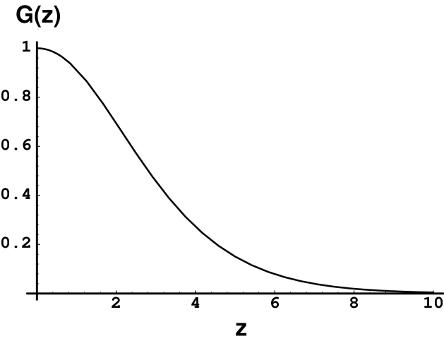
Figure 2:

Plot of the Scale Function $G(z)$ for the Open and Flat Universes.

4.2 The Closed Universe

In the case of the closed universe the spatial mode functions are the 4-dimensional spherical harmonics, which have the form [14, 17]

$$[\epsilon=1]: U_{\lambda}({\bf x})=(2\omega_{n}a^{3})^{-1/2}\,\Pi^{(+)}_{nl}(\chi)\,{\rm Y}_{lm}(\theta,\varphi),$$ (61)

$$\omega_{n}=\sqrt{{n(n+2)\over a^{2}}+\mu^{2}},$$

$$\lambda=(n,l,m).$$

Here, $n=0,1,2,\cdots;\quad l=0,1,\cdots,n;$ and $m=-l,-l+1,\cdots,+l$. The function $\Pi^{(+)}$ is found from $\Pi^{(-)}$ by replacing $\chi$ by $-i\chi$ and $q$ by $-i(n+1)$ [14]. Alternatively, they can be written in terms of Gegenbauer polynomials [17, 18] as

$$\Pi^{(+)}_{nl}(\chi)\propto\sin^{l}\chi\;{\rm C}^{l+1}_{n-l}(\cos\chi).$$ (63)

In either case, the addition theorem is found from Eq. 11.4(3) of Ref.[18] (with $p=2$ and $\xi=\eta$). This reduces to

$$\sum_{lm}|\Pi^{(+)}_{nl}(\chi){\rm Y}_{lm}(\theta,\varphi)|^{2}={(n+1)^{2}\over 2\pi^{2}}\,,$$ (64)

from which it is easy to show that the energy density inequality, Eq. (16), becomes

$$\Delta\hat{\rho}\geq-{1\over 4\pi^{2}a^{3}}\sum_{n=0}^{\infty}(n+1)^{2}\,\omega_{n}\,{\rm e}^{-2\omega_{n}t_{0}}.$$ (65)

If we use the variable $\eta={t_{0}/a}$ in the above equation, we can simplify it to

$$\Delta\hat{\rho}\geq-{3\over 32\pi^{2}t_{0}^{4}}H(\eta,\mu).$$ (66)

Again we find the flat space solution in 4 dimensions, multiplied by the scale function $H(\eta,\mu)$, which is defined as

$$H(\eta,\mu)\equiv{8\over 3}\eta^{4}\sum_{n=1}^{\infty}(n+1)^{2}\sqrt{n(n+2)+a^{2}\mu^{2}}\;{\rm e}^{-2\eta\sqrt{n(n+2)+a^{2}\mu^{2}}},$$ (67)

and is plotted in Figure 3. The scale function here has a small bump in it, occurring at roughly $\eta\approx 0.5$ with a height of 1.03245. This may permit the magnitude of the negative energy to be slightly greater for a massless scalar field in the Einstein universe than is allowed in a flat universe for comparable sampling times. A similar result was shown to exist for massive fields in a 2 dimensional Minkowski spacetime [10].

4.3 Massless asymptotic limits in the Einstein universe

As with the 3-dimensional closed universe, we can find the asymptotic limits of this function. We again follow the method of the previous section, assuming the scalar field is massless, and making use of the Plana summation formula to find

$$H(\eta,0)={8\over 3}\eta^{4}\,\bigl{(}I_{2}+I_{3}\bigr{)}\,,$$ (68)

where

$$I_{2}=\int_{0}^{\infty}(x+1)^{2}\sqrt{x(x+2)}\,{\rm e}^{-2\eta\sqrt{x(x+2)}}\,dx$$ (69)

and

$$I_{3} = 2{\rm Re}\left[i\int_{0}^{\infty}{(ix+1)^{2}\sqrt{ix(ix+2)}{\rm e}^{-2\eta\sqrt{ix(ix+2)}}\over{\rm e}^{2\pi x}-1}\,dx\right]$$ (70)

$$= \int_{0}^{\infty}\sqrt{2x}\>\frac{(x^{2}-1)\sqrt{\sqrt{x^{2}+4}+x}-2x\sqrt{\sqrt{x^{2}+4}-x}}{{\rm e}^{2\pi x}-1}\>{\rm d}x$$

$$\approx -0.356109\,.$$

The first integral can be done in terms of Struve, ${\bf H}_{n}(z)$, and Neumann, $N_{n}(z)$, functions, with the result

$$I_{2}={\pi\over 16}{d^{2}\over d\eta^{2}}\left[{1\over\eta}\left({\bf H}_{1}(2\eta)-N_{1}(2\eta)\right)\right]+\frac{4}{15}\eta\,.$$ (71)

If we follow the same procedure as in the previous section for defining the renormalized vacuum energy density for the minimally coupled scalar field in the Einstein universe, then we obtain

$$\rho_{Casimir}={1\over{4\pi^{2}a^{4}}}\,I_{3}\approx-{0.356109\over{4\pi^{2}a^{4}}}\,.$$ (72)

The same method yields $\rho_{Casimir}=1/{480\pi^{2}a^{4}}$ for the massless conformal scalar field [12]. Here our result for the minimal field, Eq. (72), differs from that obtained by Elizalde [13] using the zeta function method, $\rho^{\prime}_{Casimir}=-0.411502/{4\pi^{2}a^{4}}$. This discrepancy probably reflects the fact that the renormalized vacuum energy density is not uniquely defined. The renormalized stress tensor in a curved spacetime is only defined up to additional finite renormalizations of the form of those required to remove the infinities. In general this includes the geometrical tensors ${}^{(1)}H_{\mu\nu}$ and ${}^{(2)}H_{\mu\nu}$. (See any of the references in [19] for the definitions of these tensors and a discussion of their role in renormalization.) In the Einstein universe, both of these tensors are nonzero and are proportional to $1/a^{4}$. Thus the addition of these tensors to $\langle T_{\mu\nu}\rangle$ will change the numerical coefficient in $\rho_{Casimir}$. The logarithmically divergent parts of $\langle T_{\mu\nu}\rangle$ which are proportional to ${}^{(1)}H_{\mu\nu}$ and ${}^{(2)}H_{\mu\nu}$ happen to vanish in the Einstein universe, but not in a more general spacetime. In principle, one should imagine that the renormalization procedure is performed in an arbitrary spacetime, and only later does one specialize to a specific metric. (Unfortunately, it is computationally impossible to do this explicitly.) Thus the fact that a particular divergent term happens to vanish in a particular spacetime does not preclude the presence of finite terms of the same form.

In the small $\eta$ limit we can Taylor expand the Struve and Neumann functions in Eq. (71), and obtain

$$H(\eta,0)=1+{1\over 3}\eta^{2}+{(3+4\gamma)\over 12}\eta^{4}+{8\over 3}(-0.356109)\eta^{4}+{1\over 3}\eta^{4}\log\eta+O(\eta^{6})+\cdots,$$ (73)

where $\gamma$ is Euler’s constant, which arises in the Taylor series expansion of the Neumann function. This is similar to that of the 3-dimensional universe and again contains a term of the form of the Casimir energy. In the large $\eta$ limit we again keep just the first term of the series. Both of the asymptotic forms are plotted with the exact solution in Figure 3. We see that the asymptotic form is again a very good approximation except in the interval $1<\eta<2$, as was the case for the 3-dimensional closed universe.

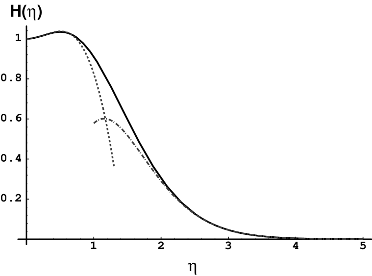
Figure 3:

The Scale Function $H(\eta)$ for the Closed Universe. The solid line is the exact result. The dotted line is the asymptotic expansion for small $\eta$, while the dot-dash curve is the large $\eta$ approximation. The maximum occurs at $\eta\approx 0.5$.

The difference inequalities for massless fields are then given by

$$\Delta\hat{\rho}\geq-{3\over{32\pi^{2}t_{0}^{4}}}\left[1+{1\over 3}\eta^{2}+{(3+4\gamma)\over 12}\eta^{4}+{1\over 3}\eta^{4}\log\eta+\cdots\right]-\rho_{Casimir}$$ (74)

for $t_{0}\ll a$ and

$$\Delta\hat{\rho}\geq-{\sqrt{3}\over{\pi^{2}a^{4}}}\,{\rm e}^{-2\sqrt{3}\,t_{0}/a}\qquad{\rm for}\quad t_{0}\gg a\,.$$ (75)

Using $\Delta\hat{\rho}=\hat{\rho}_{ren}-\hat{\rho}_{Casimir}$, where $\hat{\rho}_{Casimir}$ is the expectation value of $\rho_{ren}$ in the vacuum state, one can calculate the “total,” or more formally the renormalized energy density that would be constrained by the quantum inequalities, subject to renormalization ambiguities. For example in the 4-dimensional Einstein universe the renormalized energy density inequality is constrained by

$$\hat{\rho}_{ren}\geq-{3\over{32\pi^{2}t_{0}^{4}}}\left[1+{1\over 3}\eta^{2}+{(3+4\gamma)\over 12}\eta^{4}+{1\over 3}\eta^{4}\log\eta+O(\eta^{6})+\cdots\right]$$ (76)

for $t_{0}\ll a$. Here the coefficient of the $\eta^{4}$ term would be altered by a finite renormalization, but the rest of the expression is unambiguous. Similar expressions could be found for any of the other cases above. In the case of the flat Robertson-Walker universe, there is no Casimir vacuum energy. Under such circumstances the difference inequality and the renormalized energy density inequality are the same, and are free of ambiguities.

5 Discussion

In the previous sections, we have derived a general form for a difference inequality for a massive, minimally coupled scalar field in a static curved spacetime. This general inequality was then evaluated explicitly in a 3-dimensional closed universe and in 4-dimensional closed and open universes. The resulting inequalities include the effects of the spacetime curvature. In the small sampling time limit, they reduce to the flat space forms plus curvature-dependent corrections. These results lend support to the arguments given in Ref. [6] to the effect that this should always be the case in curved spacetime.

An additional feature of these difference inequalities is that they lead to averaged weak energy type conditions in the infinite sampling time limit. We found that in general

$$\Delta\hat{\rho}\;\equiv\;{t_{0}\over\pi}\int_{-\infty}^{\infty}{{\langle:T_{00}:\rangle dt}\over{t^{2}+t_{0}^{2}}}\;\geq-{a_{n}\over t_{0}^{n}}F_{n}(\eta)$$ (77)

where $n$ is the dimensionality of the spacetime, $a_{n}$ is the coefficient of the flat space inequality in $n$ dimensions, and $F_{n}(\eta)$ is the scale function. In all of the cases above the scale function decays exponentially to zero in the large $\eta$ limit, which is the same as the large $t_{0}$ limit. In the $t_{0}\rightarrow\infty$ limit the above expression reduces to

$$\int_{-\infty}^{\infty}\langle:T_{00}:\rangle dt=\int_{-\infty}^{\infty}\left[\langle\psi|T_{00}|\psi\rangle-\langle 0|T_{00}|0\rangle\right]dt\geq 0,$$ (78)

where $|\psi\rangle$ is an arbitrary state.

The difference inequalities are derived directly from quantum field theory and are in no way dependent upon the standard uncertainty relations. It therefore appears that quantum field theory itself leads to constraints on negative energy densities (fluxes) without any apriori assumptions. In addition, the quantum inequalities in both flat space and these generalized curved spacetimes are more restrictive on the magnitude and duration of the allowable negative energy densities than is the averaged weak energy condition. Finally it appears that the quantum inequalities themselves lead directly to AWEC type conditions in many spacetimes.

Acknowledgements

We would like to thank Thomas A. Roman for useful discussions and for help with editing the manuscript. This research was supported in part by NFS Grant No. PHY-9507351.

Appendix

In this appendix, we wish to prove the following inequality: Let $A_{ij}$ be a real, symmetric $n\times n$ matrix with non-negative eigenvalues. (For the purposes of this paper, we may take either $n=2$, for 3D spacetime, or $n=3$, for 4D spacetime.) Further let $h_{\lambda}^{i}$ be a complex $n$-vector, which is also a function of the mode label $\lambda$. Then in an arbitrary quantum state $|\psi\rangle$, the inequality states that

$${\rm Re}\sum_{\lambda,\lambda^{\prime}}A_{ij}\left[h^{i\,*}_{\lambda}h^{j}_{\lambda^{\prime}}\langle a_{\lambda}^{\dagger}a_{\lambda^{\prime}}\rangle\pm h^{i}_{\lambda}h^{j}_{\lambda^{\prime}}\langle a_{\lambda}a_{\lambda^{\prime}}\rangle\right]\geq-{1\over 2}\sum_{\lambda}A_{ij}h^{i\,*}_{\lambda}h^{j}_{\lambda}\,.$$ (A1)

In order to prove this relation, we first note that

$$A_{ij}=\sum_{\alpha=1}^{n}\kappa_{\alpha}V_{i}^{(\alpha)}\,V_{j}^{(\alpha)}\,,$$ (A2)

where the $V_{i}^{(\alpha)}$ are the eigenvectors of $A_{ij}$, and the $\kappa_{\alpha}\geq 0$ are the corresponding eigenvalues. Now define the hermitian vector operator

$$Q^{i}=\sum_{\lambda}\left(h^{i\,*}_{\lambda}a_{\lambda}^{\dagger}+h^{i}_{\lambda}a_{\lambda}\right)\,.$$ (A3)

Note that

$$\left\langle{Q^{i}}^{\dagger}A_{ij}Q^{j}\right\rangle=\sum_{\alpha=1}^{n}\kappa_{\alpha}\left\langle Q^{i\,\dagger}V_{i}^{(\alpha)}\,V_{j}^{(\alpha)}Q^{j}\right\rangle=\sum_{\alpha=1}^{n}\kappa_{\alpha}||V_{i}^{(\alpha)}\,Q^{i}|\psi\rangle||^{2}\geq 0\,.$$ (A4)

Furthermore,

$$\left\langle Q^{i\,\dagger}A_{ij}Q^{j}\right\rangle=2\,{\rm Re}\sum_{\lambda,\lambda^{\prime}}A_{ij}\left[h^{i\,*}_{\lambda}h^{j}_{\lambda^{\prime}}\langle a_{\lambda}^{\dagger}a_{\lambda^{\prime}}\rangle+h^{i}_{\lambda}h^{j}_{\lambda^{\prime}}\langle a_{\lambda}a_{\lambda^{\prime}}\rangle\right]+\sum_{\lambda}A_{ij}h^{i\,*}_{\lambda}h^{j}_{\lambda}\,,$$ (A5)

from which Eq. (A1) with the ‘$+$’-sign follows immediately. The form of Eq. (A1) with the ‘$-$’-sign can be obtained by letting $h^{j}_{\lambda}\rightarrow ih^{j}_{\lambda}$.

As a special case, we may take $A_{ij}=\delta_{ij}$ and obtain

$${\rm Re}\sum_{\lambda,\lambda^{\prime}}\left[{\bf h}_{\lambda}^{*}\cdot{\bf h}_{\lambda^{\prime}}\langle a_{\lambda}^{\dagger}a_{\lambda^{\prime}}\rangle\pm{{\bf h}_{\lambda}}\cdot{\bf h}_{\lambda^{\prime}}\langle a_{\lambda}a_{\lambda^{\prime}}\rangle\right]\geq-{1\over 2}\sum_{\lambda}|{\bf h}_{\lambda}|^{2}\,.$$ (A6)

As a further special case, we may take the vector ${\bf h}_{\lambda}$ to have only one component, e.g. ${\bf h}_{\lambda}=(h_{\lambda},0,0)$, in which case we obtain

$${\rm Re}\sum_{\lambda,\lambda^{\prime}}\left[{h_{\lambda}}^{*}h_{\lambda^{\prime}}\langle a_{\lambda}^{\dagger}a_{\lambda^{\prime}}\rangle\pm{h_{\lambda}}h_{\lambda^{\prime}}\langle a_{\lambda}a_{\lambda^{\prime}}\rangle\right]\geq-{1\over 2}\sum_{\lambda}|h_{\lambda}|^{2}\,.$$ (A7)

This last inequality was originally proven in Ref. [20] for real $h_{\lambda}$, and a simplified proof using the method adopted here is given in Ref. [10].

References

• [1] Among the numerous papers on this topic are the following: F.J. Tipler, Phys. Rev. D 17, 2521 (1978); C. Chicone and P. Ehrlich, Manuscr. Math. 31, 297 (1980); G.J. Galloway, Manuscripta Math. 35, 209 (1981); A. Borde, Class. Quantum Grav. 4, 343 (1987); T.A. Roman, Phys. Rev. D 33, 3526 (1986) and 37, 546 (1988); G. Klinkhammer, Phys. Rev. D 43, 2542 (1991); and R. Wald and U. Yurtsever, Phys. Rev D 44, 403 (1991).
• [2] L.H. Ford and Thomas A. Roman, Phys. Rev. D 51, 4277 (1995).
• [3] U. Yurtsever, Phys. Rev. D 51, 5797 (1995).
• [4] L.H. Ford, Proc. R. Soc. London A364, 277 (1978)
• [5] L.H. Ford and Thomas A. Roman, Phys. Rev. D 46, 1328 (1992).
• [6] L.H. Ford and Thomas A. Roman, Phys. Rev. D 53, 5496 (1996).
• [7] Michael J. Pfenning and L.H. Ford, manuscript in preparation.
• [8] Miguel Alcubierre, Class. Quantum Grav. 11, l73 (1994).
• [9] N.D. Birrell and P.C.W. Davies, Quantum fields in curved space, (Cambridge University Press, 1982).
• [10] L.H. Ford and Thomas A. Roman, “Restrictions on Negative Energy Density in Flat Spacetime”, Tufts University preprint, TUTP-96-2, gr-qc/960703.
• [11] See, for example, J.D. Jackson, Classical Electrodynamics, 2nd ed. (John Wiley & Sons, 1975), Eq.(3.69).
• [12] L.H. Ford, Phys. Rev. D 12, 2963 (1975).
• [13] E. Elizalde, J. Math. Phys. 35, 3308 (1994).
• [14] Leonard Parker and S.A. Fulling, Phys. Rev. D 9, 341 (1974).
• [15] E.M. Lifshitz and I.M. Khalatnikov, Adv. Phys. 12, 185 (1963), Appendix J.
• [16] T.S. Bunch, J. Phys. A 11, 603 (1978).
• [17] L.H. Ford, Phys. Rev. D 14, 3304 (1976).
• [18] A. Erdelyi, W. Magnus, F. Oberhettinger and F.G. Tricomi, Higher Transcendental Functions, Vol. II, (MacGraw-Hill, 1953).
• [19] Ref. [9], Chap. 6; S.A. Fulling, Aspects of Field Theory in Curved Space-Time, (Cambridge University Press, 1989), Chap. 9; L.H. Ford, in Cosmology and Gravitation, M. Novello, ed. (Editiones Frontières, 1994), Chap. 9.
• [20] L.H. Ford, Phys. Rev. D 43, 3972 (1991).