Evolving test-fields in a black-hole geometry

Abstract

We consider the initial value problem for a massless scalar field in the Schwarzschild geometry. When constructed using a complex-frequency approach the necessary Green’s function splits into three components. We discuss all of these in some detail: 1) The contribution from the singularities (the quasinormal modes of the black hole) is approximated and the mode-sum is demonstrated to converge after a certain well defined time in the evolution. A dynamic description of the mode-excitation is introduced and tested. 2) It is shown how a straightforward low-frequency approximation to the integral along the branch cut in the black-hole Green’s function leads to the anticipated power-law fall off at very late times. We also calculate higher order corrections to this tail and show that they provide an important complement to the leading order. 3) The high-frequency problem is also considered. We demonstrate that the combination of the obtained approximations for the quasinormal modes and the power-law tail provide a complete description of the evolution at late times. Problems that arise (in the complex-frequency picture) for early times are also discussed, as is the fact that many of the presented results generalize to, for example, Kerr black holes.

]

I Cauchy’s problem for perturbed black holes

This paper concerns the evolution of a test-field (be it scalar, electromagnetic or a perturbation of the gravitational field itself) in a spacetime that contains a black hole. That is, we consider the problem that is associated with Cauchy in the framework of general relativity. Because of the inherent nonlinearity of Einstein’s theory this problem is generally not amenable to analytic calculations. But if the wave-field is sufficiently weak that its contribution to the spacetime curvature can be neglected the evolution equations reduce to a wave equation with a complicated effective potential. This is the realm of black-hole perturbation theory [1, 2] in which the initial-value problem can be approached by “standard” methods [3, 4]. The purpose of the present work is to contribute a more detailed understanding of the many intricacies associated with the evolution of a weak wave-field in a black-hole geometry.

One can argue that this kind of discussion is of little importance to physics. It may seem obvious that much relevant information will be lost when the equations of general relativity are linearised. But it turns out that the perturbation approach provides surprisingly accurate results in many situations. An interesting example of this is the case of two colliding black holes [11]. This obviously does not mean that the linear equations render a fully nonlinear approach useless. It would be truly surprising if no new phenomena were to be unveiled by detailed nonlinear calculations, but linear studies provide important benchmarks against which such fully nonlinear, numerical calculations can (and should) be tested. Also — and of equal importance — is the fact that the linear problem can be approached “analytically”. This can lead to an improved understanding of the underlying physics and information that can be extremely difficult to infer from purely numerical data.

The problem we consider here is in many ways an old one. The evolution of a test-field in a black-hole background was first considered more than 25 years ago [12]. The general features of such an evolution are well-known [2]. The “response” of the black hole — as seen by a distant observer — can be divided into three components. Radiation emitted “directly” by the perturbation source will dominate at early times. This radiation depends on the exact character of the initial field. In contrast, the late-time response depends mainly on the parameters of the black-hole. The exponentially damped oscillations of the black-hole quasinormal modes carry a considerable part of the total radiated energy in many astrophysical processes (such as gravitational collapse) [5, 6, 7, 8]. Finally, the wave field falls off with time according to a power law at very late times [9, 10].

The initial-value problem for black-hole perturbations have been considered by several authors. In an impressive study, Leaver [3] discussed both the excitation of quasinormal modes and the nature of the power-law tails. The quasinormal-mode problem was later considered by Sun and Price [13] and also by the present author [4]. quasinormal modes in physics studied by Gundlach, Price and Pullin [14, 15] and Ching et al. [16].

Even though the problem is far from new, there are several reasons why it need be investigated further. Although the response of a black hole to an impinging wavepacket will almost exclusively be dominated by the slowest damped quasinormal modes — and present methods can reliably account for the excitation of these modes [3, 4] — several questions remain. For example: What is the role of the highly damped modes? It is known that an infinite number of quasinormal modes exist for each radiative multipole $\ell$ [17, 18], but our understanding of the role of the higher overtones is rather poor. In fact, it is not at all clear whether the mode-sum is convergent or not [3]. Our understanding of the power-law tail is also somewhat unsatisfactory. The leading behaviour has been calculated in different ways [3, 16], but the resultant formulae are only truly useful at very late times. In a typical evolution scenario there is a considerable time-window in which the signal is no longer dominated by the quasinormal modes, but the leading order power-law tail has not yet taken over. Is it possible to derive a “higher-order” tail expression that describes the evolution adequately for the intermediate times? These questions (and several others) are addressed in the present paper.

II The problem and a formal solution

A A massless scalar field in the Schwarzschild geometry

In order to make the presentation clear we have chosen to specialize this investigation to the case of a massless scalar field and Schwarzschild black holes. This is, of course, a model problem since no scalar fields have yet been observed in Nature. But this does not mean that our results are of restricted value. On the contrary: Because the equations that govern other perturbing fields (such as an electromagnetic testfield or a gravitational perturbation of the metric) are similar to the one for a scalar field [2], the results presented here are easily extended to all other relevant cases. Furthermore, as will be discussed in section VI, it seems likely that many of the present results can be adapted also to the case of rotating black holes.

In the background geometry of a Schwarzschild black hole a massless scalar field evolves according to

$$\Box\Phi=0\ .$$ (1)

Because of the underlying spherical symmetry it is meaningful to introduce the decomposition

$$\Phi_{\ell m}={u_{\ell}(r_{\ast},t)\over r}Y_{\ell m}(\theta,\varphi)\ ,$$ (2)

where $Y_{\ell m}$ are the standard spherical harmonics. The function $u_{\ell}(r_{\ast},t)$ then solves the wave equation

$$\left[{\partial^{2}\over\partial r_{\ast}^{2}}-{\partial^{2}\over\partial t^{2}}-V_{\ell}(r)\right]u_{\ell}=0\ ,$$ (3)

where the effective potential is

$$V_{\ell}(r)=\left(1-{2M\over r}\right)\left[{\ell(\ell+1)\over r^{2}}+{2M\over r^{3}}\right]\ ,$$ (4)

and $M$ is the mass of the black hole (we use geometrized units $c=G=1$). The “tortoise” coordinate $r_{\ast}$ is defined by

$${d\over dr_{\ast}}=\left(1-{2M\over r}\right){d\over dr}\ .$$ (5)

Let us now suppose that we are given a specific scalar field at some time (we will use $t=0$), and that we want to deduce the future evolution of this field. That is, we require a scheme for calculating (for each $\ell$) $u_{\ell}(r_{\ast},t)$ once we are given $u_{\ell}(r_{\ast},0)$ and $\partial_{t}u_{\ell}(r_{\ast},0)$. This problem is typically approached via a Green’s function.

B The black-hole Green’s function

It is well-known that the time-evolution of a wave-field $u_{\ell}(r_{\ast},t)$ follows immediately from

$$u_{\ell}(r_{\ast},t) = \int G(r_{\ast},y,t)\partial_{t}u_{\ell}(y,0)dy$$ (6)

$$+ \int\partial_{t}G(r_{\ast},y,t)u_{\ell}(y,0)dy\ ,$$ (7)

for $t>0$ (we will discuss the appropriate limits of integration in section IIIC). The (retarded) Green’s function is defined by

$$\left[{\partial^{2}\over\partial r_{\ast}^{2}}-{\partial^{2}\over\partial t^{2}}-V_{\ell}(r)\right]G(r_{\ast},y,t)=\delta(t)\delta(r_{\ast}-y)\ ,$$ (8)

together with the condition $G(r_{\ast},y,t)=0$ for $t\leq 0$.

To find the Green’s function $G(r_{\ast},y,t)$ is our main task. Once we know it, we can study the evolution of any initial field by evaluating the integrals in (7).

The first step in finding $G(r_{\ast},y,t)$ consists of reducing (8) to an ordinary differential equation. To do this we use the integral transform [4]

$$\hat{G}(r_{\ast},y,\omega)=\int_{0^{-}}^{+\infty}G(r_{\ast},y,t)e^{i\omega t}dt\ .$$ (9)

This transform is well defined as long as ${\rm Im}\ \omega\geq 0$, and the corresponding inversion formula is

$$G(r_{\ast},y,t)={1\over 2\pi}\int_{-\infty+ic}^{+\infty+ic}\hat{G}(r_{\ast},y,\omega)e^{-i\omega t}d\omega\ ,$$ (10)

where $c$ is some positive number.

The Green’s function $\hat{G}(r_{\ast},y,\omega)$ can now be expressed in terms of two linearly independent solutions to the homogeneous equation

$$\left[{d^{2}\over dr_{\ast}^{2}}+\omega^{2}-V_{\ell}(r)\right]\hat{u}_{\ell}(r_{\ast},\omega)=0\ .$$ (11)

The two required solutions are defined by their asymptotic behaviour. The first solution corresponds to purely ingoing waves crossing the event horizon:

$$\hat{u}_{\ell}^{\rm in}(r_{\ast},\omega)\sim\left\{\begin{array}[]{ll}e^{-i\omega r_{\ast}}\ ,&r_{\ast}\rightarrow-\infty\ ,\\ A_{\rm out}(\omega)e^{i\omega r_{\ast}}+A_{\rm in}(\omega)e^{-i\omega r_{\ast}}\ ,&r_{\ast}\rightarrow+\infty\ ,\end{array}\right.$$ (12)

and the second solution behaves as a purely outgoing wave at spatial infinity:

$$\hat{u}_{\ell}^{\rm up}(r_{\ast},\omega)\sim\left\{\begin{array}[]{ll}B_{\rm out}(\omega)e^{i\omega r_{\ast}}+B_{\rm in}(\omega)e^{-i\omega r_{\ast}}\ ,&r_{\ast}\rightarrow-\infty\ ,\\ e^{+i\omega r_{\ast}}\ ,&r_{\ast}\rightarrow+\infty\ .\end{array}\right.$$ (13)

Using these two solutions the Green’s function can be written

$$\hat{G}(r_{\ast},y,\omega)=-{1\over 2i\omega A_{\rm in}(\omega)}\left\{\begin{array}[]{lll}\hat{u}_{\ell}^{\rm in}(r_{\ast},\omega)\hat{u}_{\ell}^{\rm up}(y,\omega)\ ,&r_{\ast}<y\ ,\\ \\ \hat{u}_{\ell}^{\rm in}(y,\omega)\hat{u}_{\ell}^{\rm up}(r_{\ast},\omega)\ ,&r_{\ast}>y\ .\end{array}\right.$$ (14)

Here we have used the Wronskian relation

$$W(\omega)\equiv\hat{u}_{\ell}^{\rm in}{d\hat{u}_{\ell}^{\rm up}\over dr_{\ast}}-\hat{u}_{\ell}^{\rm up}{d\hat{u}_{\ell}^{\rm in}\over dr_{\ast}}=2i\omega A_{\rm in}(\omega)\ .$$ (15)

C Using complex frequencies

The problem can now, in principle, be approached by direct numerical integration of (11) for (almost) real values of $\omega$ and subsequent inversion of (10). This approach should lead to reliable results and an accurate representation of the evolution, as long as some obvious care is taken in each step. A multitude of examples of this approach can be found in work relating to particles orbiting black holes (see [2] for an exhaustive list of references). For the evolution of a test-field, when we want to explain why different features seen in the emerging waves arise, it may be useful to follow an alternative route, however. An approach that often proves useful when one wants to isolate the behaviour of a Green’s function in different time intervals is based on bending the integration contour in (10) into the lower half of the complex $\omega$-plane. This is the approach that we will follow here.

What do we expect to learn by analytically continuing the Green’s function in this way? First of all, it is well known that $\hat{G}(r_{\ast},y,\omega)$ has an infinite number of distinct singularities in the lower half of the $\omega$-plane. These correspond to the black-hole quasinormal modes and occur at frequencies for which the Wronskian $W(w)$ vanishes. That is, for a quasinormal mode the two solutions $\hat{u}_{\ell}^{\rm in}$ and $\hat{u}_{\ell}^{\rm up}$ are linearly dependent. To determine the quasinormal-mode frequencies is not a trivial task, but several accurate methods have been devised [19, 20, 21, 22]. The mode frequencies do not, however, contain all the information that is required to evaluate the Green’s function. While it is formally straightforward to use the residue theorem to determine the mode-contribution it is, in practice, non-trivial to evaluate the resultant expressions. One must be able to approximate the eigenfunction associated with each quasinormal mode.

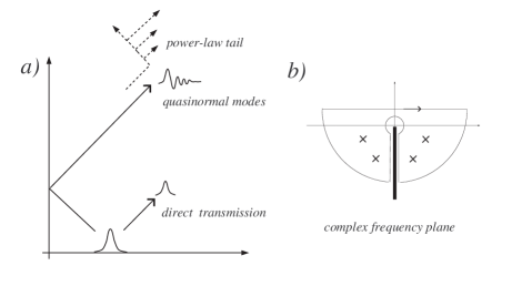
FIG. 1.: a) Schematic description of a black holes response to initial data of compact support. The directly transmitted wave (from a source point $y$) arrives at a distant observer (at $r_{\ast}$) roughly at $t-r_{\ast}+y=0$. The black holes response, that is dominated by quasinormal mode ringing, reaches the observer at roughly $t-r_{\ast}-y=0$. At very late times the signal falls off as an inverse power of time. This power-law tail arises because of multiple backscattering off the spacetime curvature. b) Integration contours in the complex frequency plane. The original inversion contour for the Green’s function lies above the real frequency axis. When analytically continued in the complex plane this contour can be replaced by the sum of 1) the quasinormal modes [the singularities of $\hat{G}(r_{\ast},y,\omega)$; the first few are represented by crosses in the figure] 2) an integral along the branch cut (a thick line along the negative imaginary $\omega$ axis in the figure), that leads to the power law tail, and 3) high frequency arcs (that one would expect vanish at most times, but they should also lead to rougly “flat space propagators” at early times).

In the complex-frequency picture the late-time power-law tail is associated with the existence of a branch cut in $\hat{u}_{\ell}^{\rm up}$. This cut is usually placed along the negative imaginary $\omega$-axis. It has been demonstrated that the behaviour at very late times can be obtained from a low-frequency approximation of the integral along the branch cut [3]. As regards the radiation that reaches an observer more or less directly from the source it has been suggested [3] that it can be associated with the large-frequency arcs that are required to “close the contour” in the complex $\omega$-plane (see Figure 1). One can argue that this should be the case in a handwaving way: For large frequencies the Green’s function limits to the familiar flat-space propagator [3]. As yet there are no detailed studies of the high-frequency problem, however.

D The asymptotic approximation

In this paper we want to pursue the problem analytically as far as possible. This means that we will often prefer a simplifying approximation over a less transparent numerical calculation. The hope is that this will lead to a reasonably accurate description of the evolution, and at the same time provide better insight into the underlying physics. Once one has acquired this understanding it will be meaningful to perform a more accurate analysis.

In this context, a useful approximation follows if one assumes that spacetime is essentially flat in the region of both the observer and the initial data (that should be of compact support). We consequently assume that i) the observer is situated far away from the black hole. This means that $r_{\ast}/M>>1$ in (14). ii) the initial data has considerable support only far away from the black hole. This implies that only the region where $y/M>>1$ contributes significantly to (7).

To make life easier we will also assume that the initial data has no support outside the observer (only $y<r_{\ast}$ are relevant). With all these restrictions the frequency-domain Green’s function (14) simplifies to

$$\hat{G}(r_{\ast},y,\omega)\approx-{1\over 2i\omega}\left[e^{i\omega(r_{\ast}-y)}+{A_{\rm out}\over A_{\rm in}}e^{i\omega(r_{\ast}+y)}\right]\ .$$ (16)

In the following we will refer to this as the “asymptotic approximation” since it follows when we use the large-argument asymptotics for $\hat{u}_{\ell}^{\rm in}$ and $\hat{u}_{\ell}^{\rm up}$ in (14). The usefulness of this approximation should be obvious.

III Quasinormal modes

A Mode-contribution to the Green’s function

As already mentioned, the quasinormal modes correspond to complex frequencies $(\omega_{n})$ for which the Wronskian $W(w)$ vanishes. This means that $A_{\rm in}(\omega_{n})=0$ and consequently it is useful to define a quantity $\alpha_{n}$ by

$$A_{\rm in}(\omega)\approx(\omega-\omega_{n})\alpha_{n}\ ,$$ (17)

in the vicinity of the mode. Then it follows from the residue-theorem (and the fact that modes in the third and fourth quadrant are in one-to-one correspondence, see Figure 4.4 in [2]) that the total contribution from the modes to the time-domain Green’s function can be written [4]

$$G^{Q}(r_{\ast},y,t)={\rm Re}\left[\sum_{n=0}^{\infty}B_{n}e^{-i\omega_{n}(t-r_{\ast}-y)}\right]\ .$$ (18)

Here we have defined

$$B_{n}={A_{\rm out}(\omega_{n})\over\omega_{n}\alpha_{n}}\ .$$ (19)

We have also used the asymptotic approximation (16), and the sum is over all quasinormal modes in the fourth quadrant. That this expression provides an accurate representation of the mode-excitation has already been demonstrated [3, 13, 4]. Typical results obtained using (18) are shown in Figures 3a-c in [4].

B Convergence of the quasinormal-mode sum

When one evolves a test-field in the Schwarzschild geometry one typically finds that the response of the black hole that is associated with the data at $y$ [cf. (7)] reaches the observer roughly when $t-r_{\ast}-y=0$. This is not too surprising: The slowest damped quasinormal modes can be associated with the peak of the effective potential [23]. Hence, one would expect the response to follow once the specific part of the initial data has had time to reach the peak of the potential (roughly at $r_{\ast}=0$) and then travel back to the observer.

An obvious question concerns the convergence of the quasinormal-mode sum (18). At what times (if any) will the sum be convergent? Previous evidence for gravitational perturbations and the first seven modes [3] suggests that the mode sum is convergent at late times, but fails to provide a lower limit of $t$ at which this convergence starts. As far a late times are concerned it is easy to convince oneself that the sum should converge: Two consecutive terms in (18) yields the ratio

$$\left[{B_{n+1}\over B_{n}}\right]e^{-i(\omega_{n+1}-\omega_{n})(t-r_{\ast}-y)}\ .$$ (20)

Now we know that [17, 18]

$$\omega_{n+1}M\approx\omega_{n}M-i/4\ ,\quad{\rm as}\quad n\to\infty\ .$$ (21)

Assuming that the term in the square brackets remains of order unity (say) it follows that the magnitude of the ratio of successive terms in the mode sum behaves asymptotically as $\exp[-(t-r_{\ast}-y)/4]$. This implies that the sum will surely converge for $t-r_{\ast}-y\gg 0$.

But this argument relies on the terms in the square brackets of (20) behaving in a certain way. Does it hold in practice? To test this we have used the approximate formulae derived in [4] to obtain $B_{n}$ for the first 200 modes of a scalar field (and $\ell=0,1$ and 2). These results are illustrated in Figure 2. The data here is not expected to be very accurate for the highly damped modes. Nevertheless, the trend is clear. The magnitude of $B_{n}$ decreases monotonically for large values of $n$. Moreover, one finds that successive terms have opposite signs. This suggests a stronger convergence than the expected one: The mode sum will converge also at $t-r_{\ast}-y=0$ .

FIG. 2.: The absolute value of the terms in the mode sum at $t-r_{\ast}-y=0$ for $\ell=0,1$ and 2 are shown as a function of the mode index $n$ for the first 200 modes. The data is obtained using approximate phase-integral expressions.

C Dynamic mode-excitation

Previous investigations of this problem [4, 13] were to a certain extent marred by what can be called the “timing problem”. Assume that the initial data consists of a “mountain” close to the black hole and a tiny “pimple” far away. It was then found that the “pimple” leads to a much larger mode-excitation than does the “mountain”. This is, of course, contrary to our expectations. Fortunately, it is also wrong.

The “timing problem” arises when one tries to associate a given set of initial data with a constant “excitation strength” of each quasinormal mode. This would be a useful approach for many familiar oscillating systems, such as a vibrating string. But this approach is probably only meaningful when the modes of the system form a complete set. In the black-hole case it is well known that the quasinormal modes are not complete (one must also take account of the branch cut integral). As we shall see, it makes more sense to consider the quasinormal-mode excitation as a dynamic process.

For example, one would not expect the quasinormal modes to be (considerably) excited until after the relevant feature in the inital data has scattered off the potential barrier that surrounds the hole. In our previous example this means that the mode-excitation that arises because of the “mountain” in the data will be relevant earlier than that associated with the “pimple”. Roughly, the modes should be excited when the relevant data reaches the peak of the effective potential ($r_{\ast}\approx 0$).

It is not very difficult to obtain a dynamic description of the mode-excitation. In fact, we need only ensure that the Green’s function respects causality. The basic “mistake” of the previous studies [4, 13] was to perform the integral over the product of the initial data and the Green’s function $\hat{G}(r_{\ast},y,\omega)$ before inverting the integral transform. If one instead uses (8) the confusion of the “timing problem” can be avoided.

To ensure causality we must ensure that the Green’s function vanishes when $t-r_{\ast}+y>0$. An observer (at $r_{\ast}$) should simply not see anything until after a signal travelling at the speed of light has been able to reach him/her from the relevant source point ($y$). In the evolution equation (8) this translates into a lower limit of integration $y=r_{\ast}-t$.

For the quasinormal modes, one can also argue for the use of an upper limit of integration: If we use (16) it is clear that the quasinormal-mode part of the signal arises from

$$G(r_{\ast},y,t)\sim-{1\over 4\pi i}\int_{C}{1\over\omega}{A_{\rm out}\over A_{\rm in}}e^{-i\omega(t-r_{\ast}-y)}d\omega\ .$$ (22)

Intuitively, one would not expect it to be meaningful to close the integration contour $C$ in the lower half-plane unless $t-r_{\ast}-y>0$. At earlier times it seems unlikely that the contribution from the necessary high-frequency arcs will vanish. We will consider this issue in more detail in section V. For now we are content to deduce that this introduces an upper limit of integration $y=t-r_{\ast}$ in the evolution equation (7).

As a simple example of the implications of this discussion we consider the static initial data

$$u(r_{\ast},0) = \exp[-0.05(r_{\ast}/M-400)^{6}]\ ,$$ (23)

$$\partial_{t}u(r_{\ast},0) = 0\ .$$ (24)

It is straightforward to multiply this data with $G^{Q}(r_{\ast},y,t)$ from (18) and then integrate (numerically) from $y=r_{\ast}-t$ to $y=t-r_{\ast}$. The result of this calculation is displayed in Figure 3. Here we have assumed that the observer sits at $r_{\ast}=500M$. This means that, according to the “dynamical” description the modes should not be present in the signal before $t\approx 950M$.

From the data presented in Figure 3 we can conclude that our approximation for the quasinormal mode ringing is quite accurate. It is conceivable that the remaining discrepancies at later times would disappear if we used the true mode-functions instead of the “asymptotic approximation”. The most interesting part of Figure 3 concerns the early times. It is notable how nicely the idea of a “dynamic” mode excitation works in practice. This allows us to discuss the relevance of the high-order modes in more detail than what has been possible before [3, 4, 13]. Since they are rapidly damped, one would expect the highly damped modes to be relevant only at early times. As can be seen in Figure 3 this is, indeed, the case. While the slowest damped mode represents the signal well after (say) $t\approx 965M$, a much better approximation (valid from (say) $t\approx 953M$) is obtained by using the sum of the first six modes. Should we include further modes in the sum this trend continues, but it becomes hard to distinguish any improvement. This evidence clearly supports the notion that the mode-sum converges for all times after $t-r_{\ast}-y=0$.

FIG. 3.: Comparing the field obtained through evolving the scalar wave equation to the approximate contribution from the quasinormal modes. The graph shows data for $\ell=2$. The solid line represents the true scalar wave, while the two dashed lines are for a) the slowest damped quasinormal mode and b) the sum of the first six modes.

IV The late-time power-law tail

It is by now well-known that the quasinormal-mode ringing is followed by a power-law tail at late times. This feature was first found in the seminal work of Price [9, 10]. Physically, the tail arises because of backscattering off the slightly curved spacetime in the region far away from the black hole [24]. This means that the tail will not depend on the exact nature of the central object. Thus, a neutron star of a certain mass will give rise to the same tail as would a black hole of the same mass.

Mathematically, it has been demonstrated that the power-law tail can be associated with the branch cut in the complex-frequency Green’s function [3]. Using this fact, the exact form of the leading order tail has been calculated in different ways. But some questions still remain. The most important one concerns the black-hole response at intermediate times — after the quasinormal modes have died away, but before the leading tail term accurately represents the evolution. Is it possible to extend existant calculations in such a way that one can approximate the evolution also at these intermediate times? Previous calculations are also somewhat involved; it would be nice to have a simpler and more direct calculation of the tail effect for black holes.

One can argue that the late-time behaviour should follow from the low-frequency contribution to the Green’s function. Basically, the effective black-hole potential in (11) will be so small for large values of $r$ that only low-frequency waves will be affected by it. Hence, a low-frequency approximation to the black-hole equation will be useful. In this section we obtain such an approximation, and use it to study the detailed behaviour of the power-law tail.

A A low-frequency approximation

Let us begin by introducing a new dependent variable

$$\hat{u}_{\ell}=\left(1-{2M\over r}\right)^{-1/2}\psi\ .$$ (25)

Then equation (11) for the scalar field becomes

$$\left[{d^{2}\over dr^{2}}+\left(1-{2M\over r}\right)^{-2}\left\{\omega^{2}-\left(1-{2M\over r}\right){\ell(\ell+1)\over r^{2}}+{M^{2}\over r^{4}}\right\}\right]\psi=0\ .$$ (26)

As already mentioned above, it is easy to argue that we only need a large $r$ approximation to account for the low-frequency response. Thus, we expand (26) as a power series in $r/M$. This leads to

$$\left[{d^{2}\over dr^{2}}+\omega^{2}+{4M\omega^{2}\over r}-{\ell(\ell+1)\over r^{2}}\right]\psi\approx 0\ .$$ (27)

The question is whether this is a useful approximation [25]. That is, is the assumption that we only need large $r$ justified? Fortunately, this is a simple thing to test. From (27) we find that the outer turning point of classical motion is located at

$$r_{tp}=2M\left\{\sqrt{{\ell(\ell+1)\over 4M^{2}\omega^{2}}-2}-1\right\}\ .$$ (28)

At $r_{tp}$ one would expect a wave with frequency $\omega$ to be scattered by the effective potential. Since $r_{tp}\to+\infty$ as $\omega M\to 0$ it is clear that the approximate equation (27) can be used with confidence for low frequencies.

Let us now introduce [26]

$$\psi=\left({r\over M}\right)^{\ell+1}e^{i\omega r}\phi(z)\ ,$$ (29)

where $z=-2i\omega r$. Then, it follows that $\phi$ should be a solution to the confluent hypergeometric equation

$$\left[z{d^{2}\over dz^{2}}+(2\ell+2-z){d\over dz}-(\ell+1-2i\omega M)\right]\phi=0\ .$$ (30)

It also follows that two basic solutions to the black-hole problem can be written (remember that $r>>2M$)

$$\hat{u}_{\ell}^{\rm in}=A\left({r\over M}\right)^{\ell+1}e^{i\omega r}M(\ell+1-2i\omega M,2\ell+2,-2i\omega r)\ ,$$ (31)

and

$$\hat{u}_{\ell}^{\rm up}=B\left({r\over M}\right)^{\ell+1}e^{i\omega r}U(\ell+1-2i\omega M,2\ell+2,-2i\omega r)\ ,$$ (32)

where $A$ and $B$ are normalisation constants. The functions $M(a,b,z)$ and $U(a,b,z)$ represent the two standard solutions to the confluent hypergeometric equation [27].

One nice feature of this approximation is that it is obvious that there will be a cut in $\hat{u}_{\ell}^{\rm up}$. We simply use the standard result [27] that, for $n$ an integer,

$$U(a,n+1,z) = {(-1)^{n+1}\over n!\Gamma(a-n)}M(a,n+1,z)\ln z+$$ (33)

$$+ \mbox{single-valued terms}\ .$$ (34)

From this it follows immediately that

$$U(a,n+1,ze^{2\pi i}) = U(a,n+1,z)$$ (35)

$$+ 2\pi i{(-1)^{n+1}\over n!\Gamma(a-n)}M(a,n+1,z)\ .$$ (36)

We will now use this result to evaluate the effect of the branch cut in the Green’s function.

B The late-time tail

We have seen that there will necessarily be a branch cut in the black-hole Green’s function $\hat{G}(r_{\ast},y,\omega)$ (or more specifically, in the solution $\hat{u}_{\ell}^{\rm up}$). To arrive at the detailed power-law tail we need to consider the effect of this cut. It is easy to see that the contribution from the branch cut follows from the integral [cf. (10)]

$$G^{C}(r_{\ast},y,t)=$$ (37)

$${1\over 2\pi}\int_{0}^{-i\infty}\hat{u}_{\ell}^{\rm in}(y,\omega)\left[{\hat{u}_{\ell}^{\rm up}(r_{\ast},\omega e^{2\pi i})\over W(\omega e^{2\pi i})}\right.$$ (38)

$$\quad\quad-\left.{\hat{u}_{\ell}^{\rm up}(r_{\ast},\omega)\over W(\omega)}\right]e^{-i\omega t}d\omega\ .$$ (39)

After some straightforward steps this can be rewritten as

$$G^{C}(r_{\ast},y,t)=$$ (40)

$${1\over 2\pi}\int_{0}^{-i\infty}\hat{u}_{\ell}^{\rm in}(y,\omega)\hat{u}_{\ell}^{\rm in}(r_{\ast},\omega)\times$$ (41)

$$\quad\quad\times{W[\hat{u}_{\ell}^{\rm up}(r_{\ast},\omega),\hat{u}_{\ell}^{\rm up}(r_{\ast},\omega e^{2\pi i})]\over W(\omega e^{2\pi i})W(\omega)}e^{-i\omega t}d\omega\ .$$ (42)

Using the low-frequency approximation that was described in the previous section we can show that

$$W(\omega)=(-1)^{-\ell-1}iAB{(2\ell+1)!(2\omega)^{-2\ell-1}\over\Gamma(\ell+1-2i\omega M)}\ ,$$ (43)

and since there is no cut in $\hat{u}_{\ell}^{\rm in}$ it is easy to see from (36) that

$$W(\omega e^{2\pi i})=W(\omega)\ .$$ (44)

To build the Green’s function we also need

$$W[\hat{u}_{\ell}^{\rm up}(r_{\ast},\omega),\hat{u}_{\ell}^{\rm up}(r_{\ast},\omega e^{2\pi i})]=$$ (45)

$$\quad B^{2}{(-1)^{-\ell-1}2\pi(2\omega)^{-2\ell-1}\over\Gamma(-\ell-2i\omega M)\Gamma(\ell+1-2i\omega M)}\ .$$ (46)

If we use these results together with the approximation

$$\hat{u}_{\ell}^{\rm in} \approx A\left({r\over M}\right)^{\ell+1}e^{i\omega r}M(\ell+1,2\ell+2,-2i\omega r)=$$ (47)

$$= A(2\ell+1)!!(\omega M)^{-\ell}\left({r\over M}\right)j_{\ell}(\omega r)\ ,$$ (48)

we get

$$G^{C}(r_{\ast},y,t)=4iMr_{\ast}y\int_{0}^{-i\infty}\omega^{2}j_{\ell}(\omega r_{\ast})j_{\ell}(\omega y)e^{-i\omega t}d\omega\ .$$ (49)

To obtain this result we have assumed that the asymptotic approximation is valid. Specifically, we have replaced $r$ by $r_{\ast}$. This is not at all a necessary step, but it simplifies the comparison to our numerical evolutions of (3) which were carried out using $r_{\ast}$ as independent variable. Moreover, if $r$ is sufficiently large we will only introduce a small error. In the specific case of (24) the error introduced in this way will be smaller than 2.5 % .

As long as we are only interested in the leading order behaviour at very late times, we can assume that $\omega y<\omega r_{\ast}<<1$ [3]. Thus, using the standard power series expansion for $j_{\ell}(z)$ we arrive at the final formula

$$G^{C}(r_{\ast},y,t)=(-1)^{\ell+1}{(2\ell+2)!\over[(2\ell+1)!!]^{2}}{4M(r_{\ast}y)^{\ell+1}\over t^{2\ell+3}}\ .$$ (50)

This result is identical to that obtained by Leaver [3]. This is not surprising since our derivation is just a simplification of Leaver’s approach. Our result also agrees with that of Ching et al [16], but in that case one must do some additional calculations to obtain the explicit result for the black-hole case.

We have not yet contributed much new information. The greatest merit of the above derivation is its simplicity. The origin of the branch cut is clear and its contribution to the Green’s function follows painlessly. This is in remarkable contrast to, for example, the work of Ching et al [16], where the result follows after a truly involved analysis. On the other hand, the formulae obtained by Ching et al. are valid for a large class of potentials. Hence, their work shows that the tail-phenomenon is a generic feature of many problems in wave scattering.

Simplicity is not the sole advantage of the present approach, however. It turns out that we can easily do the full integral in (49). As long as $t-r_{\ast}-y>0$ we can employ equation (6.626) from Gradshteyn and Ryzhik [29]. This leads to a higher-order result

$$G^{C}(r_{\ast},y,t)=$$ (51)

$$M\sum_{m=0}^{\infty}\sum_{n=0}^{m}{(-1)^{\ell+1}2^{2-m}(2\ell+2m+2)!\over n!(m-n)!(2\ell+2n+1)!!(2\ell+2m-2n+1)!!}\times$$ (52)

$$\quad\quad\times{r_{\ast}^{\ell+2m-2n+1}y^{\ell+1+2n}\over t^{2\ell+3+2m}}\ ,$$ (53)

which is remarkably simple.

FIG. 4.: Comparing the field obtained through evolving the scalar wave equation to the approximate contribution from the power-law tail. The graph shows data for $\ell=2$ using a logarithmic scale. The solid line represents the true scalar wave, while the three dashed lines are for a) the leading order power-law tail b) the tail approximation including the first two terms and c) using the first 11 terms in the tail-sum.

We have thus managed to extend previous work to include higher order corrections to the power-law tail. The question is to what extent such a result is useful. Interestingly, it turns out that the higher order terms play an important role. Essentially they allow us to extend the validity of the tail-approximation to much earlier times. A typical result — obtained for the initial data given in (24) — is shown in Figure 4. Although it is not clear from Figure 4, it can be verified that the lowest order tail-term is a reasonable approximation to the true evolution at very late times. But the improvement achieved by including the first two terms in (53) is impressive. It is also clear from Figure 4 that if one includes several terms in (53) one arrives at an approximation that takes over from the quasinormal-mode ringing in a natural way.

Figure 4 shows that there will be a considerable time window in which the contributions from the quasinormal-modes and the higher order tail are of the same order of magnitude. It seems reasonable to assume that this may lead to interference effects that can be distinguished in the evolution of the field. That such effects are present is clear from Figure 5. It is also clear that a combination of the quasinormal modes and the higher order tail-sum provides a good representation of the evolution throughout the transition between the typical times when either term dominates the signal. Thus the approximations discussed so far can be combined to estimate the signal for all times $t-r_{\ast}-y>0$.

FIG. 5.: Comparing the field obtained through evolving the scalar wave equation to the approximate contribution from the slowest damped quasinormal mode and the first 11 terms in the sum for the power-law tail. The graph shows data for $\ell=2$ using a logarithmic scale. The solid line represents the true scalar wave, while the dashed line represents the approximation. It is easy to distinguish effects of interference between the mode and the tail-terms (whenever the ringing differs from pure expontential damping at a constant oscillation frequency).

V High frequencies

In the complex-frequency approach it is typically assumed that the contribution from the required arcs at $|\omega|\to\infty$ is irrelevant. That way, the original contour-integral can often be replaced by a mode-sum such as (18). In the black-hole problem the situation is, of course, complicated by the branch cut in the Green’s function. But as we have seen, the contribution from this cut can readily be approximated (at least at late times). To complete the study of the initial value problem we now focus our attention on the high-frequency problem.

Although it is easy to give a handwaving argument that suggests that the large-frequency arcs should not contribute significantly to the Green’s function (when $|\omega M|$ is very large one would not expect the details of the effective potential to matter much; a high-frequency wave will propagate almost as in flat space) the issue has not been studied in much detail previously. A better understanding of the high-frequency problem is useful for several reasons: i) We obviously should confirm that our expectations of a vanishing contribution to the Green’s function holds. ii) The high frequencies may hold the key to the response of the black hole at early times [3]. Hence, it is plausible that an understanding of the behaviour for high frequencies will yield a handle on the inital part of the signal that reaches an observer.

A An approximation for high frequencies

An approximation that is relevant for high frequencies can be obtained in the following way : When $|\omega M|$ becomes large the equation that governs the scalar field (26) limits to the confluent hypergeometric equation [28]

$$\left[z{d^{2}\over dz^{2}}+(2\mu-z){d\over dz}-(\mu-2i\omega M)\right]\phi=0\ .$$ (54)

Here we have used

$$\psi=\left({r\over 2M}-1\right)^{\mu}\exp\left[i\omega(r-2M)\right]\phi\ ,$$ (55)

$$z=-2i\omega(r-2M)\ ,$$ (56)

and $\mu$ is given by

$$\mu={1\over 2}-2i\omega M\ .$$ (57)

As in the case of low frequencies it is easy to use standard formulae from [27] and show that the two basic solutions that we require to build the black-hole Green’s function can be written

$$\hat{u}_{\ell}^{\rm in}=\left({r\over 2M}\right)^{1/2}\left({r\over 2M}-1\right)^{-2i\omega M}\times$$ (58)

$$\times M(1/2-4i\omega M,1-4i\omega M,-2i\omega(r-2M))e^{i\omega(r-4M)}\ ,$$ (59)

and

$$\hat{u}_{\ell}^{\rm up}=(-4i\omega M)^{1/2-4i\omega M}\left({r\over 2M}\right)^{1/2}\left({r\over 2M}-1\right)^{-4i\omega M}\times$$ (60)

$$\times U(1/2-4i\omega M,1-4i\omega M,-2i\omega(r-2M))e^{i\omega r_{\ast}}\ .$$ (61)

From the asymptotic behaviour of the confluent hypergeometric functions [27] it follows that (in the right half of the complex $\omega$-plane)

$$A_{\rm out}={\Gamma(1-4i\omega M)(4i\omega M)^{-1/2+4i\omega M}e^{-4i\omega M}\over\sqrt{\pi}}\ ,$$ (62)

and

$$A_{\rm in}={\Gamma(1-4i\omega M)(4i\omega M)^{-1/2}e^{i\pi/2}\over\Gamma(1/2-4i\omega M)}\ .$$ (63)

After using large argument approximations for the $\Gamma$ functions we get

$$A_{\rm out}\approx i\sqrt{2}e^{-4\pi\omega M}\ ,$$ (64)

and

$$A_{\rm in}\approx 1\ .$$ (65)

Hence, a high-frequency approximation to the “reflection coefficient” of the black hole is

$${\cal R}=|{A_{\rm out}\over A_{\rm in}}|^{2}\approx e^{-8\pi\omega M}\ .$$ (66)

This result agrees with our expectations (from for example the WKB method): For very large frequencies the reflection caused by the black-hole potential barrier will be exponentially small.

We can also use this approximation to approximate the very high overtones of the black hole. Recall that the quasinormal modes follow from $A_{\rm in}=0$. Then, it is trivial to use (63) and show that modes should be located at [28]

$$\omega_{n}M=-{i\over 4}\left(n+{1\over 2}\right)\ .$$ (67)

This approximation yields the correct damping rate for the high modes, but it fails to reproduce the small constant real part that each mode should have [17, 18].

B High-frequency Green’s function

We now want to use these results to discuss the possible contribution to the black hole Green’s function from the required arcs at $|\omega M|\to\infty$. To do this we assume that the asymptotic approximation from section IID is appropriate (we will discuss alternatives to this later). Then we clearly get (in the right half-plane)

$$\hat{G}^{\infty}(r_{\ast},y,\omega)\approx-{1\over 2i\omega}\left[e^{i\omega(r_{\ast}-y)}+i\sqrt{2}e^{-4\pi\omega M}e^{i\omega(r_{\ast}+y)}\right]\ .$$ (68)

For obvious reasons it makes sense to study the two terms in the square brackets separately.

For each term we require an integral of form [ cf. (10)]

$$I=\int_{C}{f(\omega)\over\omega}e^{-i\omega\tau}d\omega\ ,$$ (69)

where $C$ is a large-frequency quarter circle in either the upper or the lower right half of the $\omega$-plane (the calculation here must be complemented by similar formulae for the left half-plane). Now, as long as

$${f(\omega)\over\omega}\to 0\ ,\quad{\rm as}\quad|\omega|\to\infty\,$$ (70)

(which is certainly true here) the integral $I$ vanishes i) in the upper half-plane for $\tau<0$, and ii) in the lower half-plane for $\tau>0$ (Jordan’s lemma).

For the specific case of the black-hole Green’s function this means that

$$G(r_{\ast},y,t)=0\ ,\quad{\rm for}\quad\left\{\begin{array}[]{ll}&t-r_{\ast}+y<0\ ,\\ &t-r_{\ast}-y>0\ .\end{array}\right.$$ (71)

This is a nice result because it shows that a combination of the quasinormal modes and the contribution from the branch cut in $\hat{G}(r_{\ast},y,\omega)$ should form a complete description of the wave evolution after $t-r_{\ast}-y=0$. This confirms the result of the previous section. It also shows that the evolution should be causal: No signal will reach the observer before $t-r_{\ast}+y=0$. But the situation for the intermediate times is not clear.

C Approximating the signal at earlier times

We have seen (cf. Figure 5) that the combination of the quasinormal modes and the higher order tail sum provides a complete description of the evolution of an initial wave field after a certain time. The only remaining question is whether we can approximate the evolution adequately also at earlier times. Unfortunately, this turns out to be harder than what one might expect.

To discuss this issue we consider the high-frequency Green’s function (68). For intermediate times $r_{\ast}-y\leq t\leq r_{\ast}+y$ one would naively want to use a contour in the lower half-plane for the first term in (68) while at the same time using a contour in the upper half-plane for the second term. But although consistent with our discussion of quasinormal modes in section III this is not a useful approach. The main reason is that we should not treat the two terms in (68) independently. This does not mean that our previous discussion is flawed: Our results still hold because after $t-r_{\ast}-y>0$ one would certainly want to close both integration contours in the lower half-plane. But problems arise when we want to consider earlier times.

Before discussing this problem in more detail it may be helpful to illustrate the features in the evolution that we want to describe. In Figure 6 we show the initial signal that reaches the observer (at $t-r_{\ast}+y=0$) in the case of (24). It is clear that this signal is more or less the direct transmission that one would expect in flat space. But there is one important difference that is hard to distinguish in Figure 6: After the initial pulse follows a tiny wake. A description of the early time behaviour must yield this effect. Another part of the signal that one would like to describe is the “reflected” pulse that reaches the observer slightly before $t-r_{\ast}-y=0$, i.e., before the onset of quasinormal ringing in Figure 3.

So why is this problem difficult? Basically, there are two possible routes and both forces us to deal with formally singular terms. The first possibility is to close the integration contour in the upper half-plane at all times before $t-r_{\ast}-y=0$. If we do so it is clear that the first term in (68) will be singular, but all other contributions to the Green’s function will vanish. The second option is to close the contour in the lower half-plane as early as $t-r_{\ast}+y=0$. Then we find that there will be three divergent terms (that must balance each other in some magic way): We know that the quasinormal-mode sum will diverge, and the same is true also for the integral along the branch cut and the high-frequency arc [the second term in (68)]. Clearly, this second alternative is the less attractive one and we will take a few steps down the first route here.

FIG. 6.: Comparing the field (for $\ell=2$) obtained through evolving the scalar wave equation to an approximation that corresponds to propagation in flat space. The initial signal that reaches the observer is shown. After the, essentially unchanged, initial shape follows a tiny wake. This wake will be more pronounced for data that has support closer to the black hole. The solid line represents the true scalar wave, while the dashed line represents the approximation.

Let us consider only the leading order. As already pointed out, the only contribution to the Green’s function that does not vanish for $r_{\ast}-y\leq t\leq r_{\ast}+y$ comes from the first term in (68). Thus, we need to evaluate

$$G(r_{\ast},y,t)=-{1\over 4\pi i}\int_{C}{e^{-i\omega(t-r_{\ast}+y)}\over\omega}d\omega\ ,$$ (72)

where the integration contour $C$ is a semi-circle in the upper half-plane. Now the integrand can be identified as the Laplace-transform of the step-function. Specifically, we get

$$G(r_{\ast},y,t)={1\over 2}H(t-r_{\ast}-y)\ .$$ (73)

This is, of course, exactly what we would get in flat space. To understand the added subtleties of the black-hole case we must pursue the calculation to higher orders.

In principle, such a higher order calculation seems possible. One could, for example, try to express the high-frequency approximations of the solutions $\hat{u}_{\ell}^{\rm up}$ and $\hat{u}_{\ell}^{\rm in}$ from section VA as power series in $\omega^{-n}$. That should yield higher order corrections to (73). Unfortunately, it seems as if one would have to keep a large number of terms (all?) in the resultant expression to get a useful answer. There may also be less obvious complications. Hence, we will have to return to this problem in the future.

VI Extending the present work

To conclude this paper it is meaningful to discuss how the present work — for a massless scalar field in the Schwarzschild geometry — can be adapted to other, physically more interesting, cases.

A Other perturbing fields

The simplest extension of the present work regards other perturbing fields. It is, in fact, trivial to show that all our results carry over also to electromagnetic and gravitational waves in the Schwarzschild background. Both the discussion of the tail effect in section IV and the high-frequency discussion in section V are valid also for these other test-fields. As regards the quasinormal modes, the characteristic frequencies (and the coefficients $B_{n}$ in (18)) will be different for other fields, but the approximate phase-integral expressions [4] that we used to evaluate (18) can be used also for electromagnetic and gravitational perturbations.

B Without the asymptotic approximation

Throughout this paper we used the asymptotic approximation from section IID to simplify the calculations. This clearly restricts the initial data in an unneccessary way. Fortunately, it is not (formally) difficult to generalize our results in such a way that they hold also for more general data. First we note that the asymptotic approximation was never used (apart from in the replacement of $r$ by $r_{\ast}$ in (49)) in the derivation of the tail-expressions. Consequently, these results remain unchanged also for general initial data. For the quasinormal modes, we must use approximations of the corresponding eigenfunctions that remain valid for all $r$. That this can be done has already been demonstrated by Leaver [3]. The dynamic mode-excitation from section IIIC becomes more difficult to introduce in the general case. With the asymptotic approximation it was easy to find a time before which it would be meaningless to use integration contours in the lower half of the $\omega$-plane. In the general case, this specific time might not be so easy to define. This issue is intimately related to the high-frequency problem. It is clear that the asymptotic approximation is crucial for the discussion in section VB. In the general case one should use large-$\omega$ asymptotics for (59) and (61) that do not at the same time assume a large value of $r$. Such asymptotic expressions are not standard but they should be possible to derive [30]. These new approximations should indicate at what time it is sensible to use integration contours in the lower half of the $\omega$-plane, and thus imply an initial time for the excitation of quasinormal modes. Consequantly, it seems likely that all the ideas presented in this paper can be useful also in the general case.

C Rotating black holes

We finally turn to the problem for rotating black holes. When the black hole is rotating both the angular and the radial functions that are required to describe a perturbation are frequency-dependent. In a numerical evolution one would therefore not decouple the corresponding equations, and thus have to deal with a two-dimensional problem. The analysis of the Kerr problem is, in general, far more complicated than the present one. But in principle one would expect all the ideas discussed in this paper to be useful also for rotating holes.

For example, the construction of the black hole Green’s function should be analogous to that in section II. Of course, the angular dependence would have to be included in equations like (7). Then the quasinormal modes are defined exactly as in the Schwarzschild case. The main difference is that each Schwarzschild mode splits into $2\ell+1$ distinct ones (for different values of $m$) because of the rotation of the black hole [19].

As regards the late-time power-law tail, the generalization to Kerr also seems straightforward. Since the issue of tails in the geometry of a rotating black hole has recently been analyzed through numerical evolutions by Krivan, Laguna and Papadopoulos [31] it may be worthwhile to discuss this in somewhat more detail here.

As was first shown by Teukolsky, the equations that govern a small perturbation of a rotating black hole can be written [32]

$$\Delta^{-s}{d\over dr}\left(\Delta^{s+1}{dR\over dr}\right)$$ (74)

$$\quad+\left[{K^{2}-2is(r-M)K\over\Delta}+4is\omega r-\lambda\right]R=0\ ,$$ (75)

and

$${1\over\sin\theta}{d\over d\theta}\left(\sin\theta{dS\over d\theta}\right)+\left[a^{2}\omega^{2}\cos^{2}\theta-{m^{2}\over\sin^{2}\theta}-2a\omega s\cos\theta\right.$$ (76)

$$\left.-{2ms\cos\theta\over\sin^{2}\theta}-s^{2}\cot^{2}\theta+E-s^{2}\right]S=0\ .$$ (77)

Here we have introduced

$$K\equiv(r^{2}+a^{2})\omega-am\ ,$$ (78)

and

$$\lambda\equiv E-s(s+1)+a^{2}\omega^{2}-2am\omega\ .$$ (79)

Here $a\leq M$ is the rotation parameter of the black hole, and $s$ is the spin-weight of the perturbing field. The solutions to the angular equation (77) are generally referred to as “spin-weighted speroidal harmonics”.

Let us now adopt the approach of section IV and approach the Kerr problem for low frequencies. It is sufficient to consider $s\geq 0$ (the results for $s=-1,-2$ can be deduced via the Teukolsky-Starobinsky identities [1]), and we can also use the fact that [33]

$$E=\ell(\ell+1)+s^{2}+\sum_{n=1}^{\infty}f_{n}(a\omega)^{n}\ .$$ (80)

Then we expand (75) for large $r$ and find

$${d^{2}\psi\over dr^{2}}+\Bigl{[}\omega^{2}+{4M\omega^{2}+2is\omega\over r}$$ (81)

$$-{\ell(\ell+1)+s^{2}-12M^{2}\omega^{2}+2am\omega-2isM\omega\over r^{2}}\Bigr{]}\psi=0\ ,$$ (82)

where the new dependent variable $\psi$ is defined by $R=\Delta^{-(s+1)/2}\psi$. From this equation two things follow immediately: i) For low frequencies we can neglect all frequency dependent terms in the factor of $1/r^{2}$. ii) For scalar waves ($s=0$) we reproduce the Schwarzschild equation (27). Hence, the leading-order tail calculation in section IV must remain valid also for scalar waves in the Kerr background. This confirms the main result of Krivan, Laguna and Papadopoulos [31]. But what about fields with non-zero $s$? Well, from (77) and (82) follows that we can neglect all terms that depend on the rotation of the black hole. This shows that it is sufficient to analyze the tail effect in the Schwarzschild limit. The fact that the radial equation (82) does not immediately agree with (27) need not worry us too much. As Chandrasekhar has shown [34], the $a\to 0$ limit of (75) — the Bardeen-Press equation [35] — can easily be transformed into the Regge-Wheeler equation (11). We thus have clear evidence that the leading order tail result from section IV will hold also for Kerr black holes.

To derive higher order tail-corrections for Kerr demands a more involved analysis. The issue is complicated by the frequency-dependent coupling between (75) and (77). Similar difficulties make the high-frequency problem less transparent. Hence, we will not discuss these problems further here. What is clear is that the Kerr problem poses an interesting challenge, and we hope to be able to discuss it further in the near future.

REFERENCES

- [1] S. Chandrasekhar The mathematical theory of black holes (Oxford University Press 1983).
- [2] N. Andersson, Black-hole perturbations, Chapter 4 in Physics of black holes by I.D. Novikov and V. Frolov (Kluwer Academic Publishers 1996).
- [3] E.W. Leaver, Phys. Rev. D 34 384 (1986).
- [4] N. Andersson, Phys. Rev. D 51 353 (1995).
- [5] C.T. Cunningham, R.H. Price and V. Moncrief Ap. J. 224 643 (1978).
- [6] C.T. Cunningham, R.H. Price and V. Moncrief Ap. J. 230 870 (1979).
- [7] E. Seidel Phys. Rev. D 42 1884 (1990).
- [8] E. Seidel Phys. Rev. D 44 950 (1991).
- [9] R.H. Price Phys. Rev. D 5 2419 (1972).
- [10] R.H. Price Phys. Rev. D 5 2439 (1972).
- [11] R.H. Price and J. Pullin, Phys. Rev. Lett. 72 3297 (1994).
- [12] C.V. Vishveshwara, Nature 227 936 (1970).
- [13] Y. Sun and R.H. Price, Phys. Rev. D 38 1040 (1988).
- [14] C. Gundlach, R.H. Price and J. Pullin, Phys. Rev. D 49 883 (1994).
- [15] C. Gundlach, R.H. Price and J. Pullin, Phys. Rev. D 49 890 (1994).
- [16] E.S.C. Ching, P.T. Leung. W.M. Suen and K. Young, Phys. Rev. D 52 2118 (1995).
- [17] H-P. Nollert, Phys. Rev. D 47 5253 (1993).
- [18] N. Andersson, Class. Quantum Grav. 10 L61 (1993).
- [19] E.W. Leaver Proc. R. Soc. London A 402 285 (1985).
- [20] N. Andersson Proc. R. Soc. London A 439 47 (1992).
- [21] N. Andersson and S. Linnæus Phys. Rev. D 46 4179 (1992).
- [22] H-P. Nollert and B.G. Schmidt, Phys. Rev. D 45 2617 (1992).
- [23] B.F. Schutz and C.M. Will Ap. J. 291 L33 (1985).
- [24] K.S. Thorne p. 231 in Magic without magic: John Archibald Wheeler Ed: J. Klauder (W.H. Freeman, San Francisco 1972)
- [25] It should be clear that this low-frequency approximation can be used only for . The special case of must be considered separately. This has been done by Ching et al. [16].
- [26] J.A.H. Futterman, F.A. Handler and R.A. Matzner Scattering from black holes (Cambridge Univ. Press 1988).
- [27] M. Abramowitz and I.A. Stegun, Handbook of mathematical functions (Dover Publications, New York 1970).
- [28] H. Liu and B. Mashhoon, Class. Quantum. Grav. 13 233 (1996).
- [29] I.S. Gradshteyn and I.M. Ryzhik, Table of integrals, series and products (Academic Press, London 1980)
- [30] R. Capon private communication
- [31] W. Krivan, P. Laguna and P. Papadopoulos Dynamics of scalar fields in the background of rotating black holes preprint (1996).
- [32] S.A. Teukolsky Ap. J. 185, 635 (1973).
- [33] E. Seidel Class. Quantum Grav. 6, 1057 (1989).
- [34] S. Chandrasekhar Proc. R. Soc. London A343, 289 (1975).
- [35] J.M. Bardeen and W.H. Press J. Math. Phys. 14, 7 (1973).