Strong Cosmic Censorship and Causality Violation

Abstract

We investigate the instability of the Cauchy horizon caused by causality violation in the compact vacuum universe with the topology $B\times\,{\bf S}^{1}\times{\bf R}$, which Moncrief and Isenberg considered. We show that if the occurrence of curvature singularities are restricted to the boundary of causality violating region, the whole segments of the boundary become curvature singularities. This implies that the strong cosmic censorship holds in the spatially compact vacuum space-time in the case of the causality violation. This also suggests that causality violation cannot occur for a compact universe.

Department of Physics, Tokyo Institute of
Technology, Oh-Okayama Meguro-ku, Tokyo 152, Japan

Pacs number(s): 04.20.-q 04.20.Gz 04.20.Dw 98.80.Hw

I Introduction

Whether space-time is allowed to have causality violating regions or not is an important problem in classical general relativity. Tipler [1, 2] showed that any attempt to evolve closed timelike curves from an initial regular Cauchy data would cause singularities to form in a space-time. Kriele [3] showed that the causality violating set has incomplete null geodesics if its boundary is compact. Maeda and Ishibashi [4] showed that singularities necessarily occur when a boundary of causality violating set exists in a space-time under the physically suitable assumptions. Thus, over the past few decades a considerable number of studies have been made to elucidate the relations between causality violation and singularities.

The appearance of causality violation causes the Cauchy horizon. This is closely related to the strong cosmic censorship. Its mathematical description is that the maximal globally hyperbolic development of a generic initial Cauchy data is inextendible [5]. In other words, it holds if a space-time admits no Cauchy horizon. So far only few attempts have been made to study the instability of the Cauchy horizon due to causality violation in classical general relativity.

One can observe the appearance of causality violations and associated Cauchy horizons in compact universe models by extending the space-time maximally. The Taub-NUT universe is one of such models. In the compact homogeneous vacuum universe case, Chruściel and Rendall [6] showed that the strong cosmic censorship holds in a few class of Bianchi types. Ishibashi et al. [7] showed that the strong cosmic censorship holds in compact hyperbolic inflationary universe models.

On the other hand Moncrief and Isenberg [8] showed that causality violating cosmological solutions of Einstein equations are essentially artifacts of symmetries. They proved that there exists a Killing symmetry in the direction of the null geodesic generator on the Cauchy horizon if the Cauchy horizon is compact by using Einstein equations. We can easily understand this curious result by inspecting exact solutions which have causality violating regions. For example, the Misner space-time and the Taub-NUT universe, which have compact Cauchy horizons, have Killing symmetries on the Cauchy horizons. However, the physically realistic universe is inhomogeneous and does not admit Killing symmetries. Thus we expect that compact inhomogeneous universe does not have any Cauchy horizon or, if it does, the Cauchy horizon cannot be compact from the results of Moncrief and Isenberg. One often studies inhomogeneous universe by adding perturbations on homogeneous models. Especially there are some works on the perturbative analysis of spatially compact universe with a compact Cauchy horizon. As one of such perturbative approaches, Konkowski and Shepley [9] studied two dimensional cylindrical vacuum space-times. They demonstrated the tendency of appearing of scalar curvature singularities on the Cauchy horizon (see also Ref.[10]). These investigations suggest that, if spatially compact universe has a Cauchy horizon which divides the space-time into causality preserving region and violating region, scalar curvature singularities occur somewhere on the Cauchy horizon.

In this paper we present a theorem as our main result in which if spatially compact universe satisfies generic conditions and, if any, all the occurring curvature singularities are restricted to the boundaries of causality violating regions, then the whole segments of the Cauchy horizon become curvature singularities. Consequently it follows that such a universe cannot be extended to the causality violating regions.

In the next section, we shall classify Cauchy horizons in the compact universe into two categories and introduce the definitions for discussing causal structure and singularities. In section 3, we briefly review the result of Moncrief and Isenberg [8], by introducing Gaussian null coordinates. We also review the dual null formalism of Hayward [11] for proving our theorem. We present our theorem in section 4. Section 5 is devoted to summary and discussion on the strong curvature singularity.

II Chronological Cauchy horizon

In general, one can classify the Cauchy horizons in the spatially compact space-times into the following two types. Fig. 1 (a) shows the Cauchy horizon which is caused by a singularity. Fig. 1 (b) shows the Cauchy horizon which is caused by causality violation, where the light corn is tipped allowing the existence of the closed null geodesic generators. The other types of Cauchy horizon, for example, that is caused by timelike null-infinity, cannot occur in the case of spatially compact space-time under consideration. The most distinct feature of the two Cauchy horizons is whether the null geodesic generators are closed or not. More precisely, in Fig. 1 (a) the null geodesic generators have future endpoints but in Fig. 1 (b) they do not. Moncrief and Isenberg [8] have considered the case of Fig. 1 (b). Their geometrical assumption is the following; Let the space-time be $(M,g)$ such as $M=\Sigma\times{\bf R}$ where $\Sigma$ is a compact three manifold and the metric $g$ is analytic. If there exists a Cauchy horizon $H^{+}(S)$ of a partial Cauchy surface $S$, then $H^{+}(S)$ is a compact null embedded hypersurface which is diffeomorphic to $\Sigma$ and the topology of $H^{+}(S)$ is $B\times\,{\bf S}^{1}$, where $B$ is a compact spacelike two-manifold and the ${\bf S}^{1}$ factor is generated by the closed null geodesic generator of $H^{+}(S)$. More precisely, they considered such a Cauchy horizon $H^{+}(S)$ with a local product bundle structure in the sense that;
if $H^{+}(S)$ contains a closed null geodesic generator $\gamma$, there exists an open set $U_{\gamma}$ containing $\gamma$ such that
(i) $U_{\gamma}\cap H^{+}(S)$ is diffeomorphic to $B_{\gamma}\times{\bf S}^{1}$ for some two-manifold $B_{\gamma}$ and some diffeomorphism $\phi_{\gamma}:U_{\gamma}\cap H^{+}(S)\rightarrow B_{\gamma}\times{\bf S}^{1}$, and
(ii) there is a smooth, surjective map $\pi_{\gamma}:B_{\gamma}\times{\bf S}^{1}\rightarrow B_{\gamma}$ such that, for any $p\in B_{\gamma}$, $B_{\gamma}\times{\bf S}^{1}\approx B_{\gamma}\times\pi^{-1}_{\gamma}(p)$ and the fiber $\pi^{-1}_{\gamma}(p)$ is diffeomorphic to a closed null generator lying in $U_{\gamma}\cap H^{+}(S)$.

The set of the type $U_{\gamma}\cap H^{+}(S)$ is called the elementary region of $H^{+}(S)$.

They showed that a compact null hypersurface $H^{+}(S)$ has an analytic Killing field $Y$ which is null and tangents to a null geodesic generator of $H^{+}(S)$. This interesting fact is due to the compactness of $H^{+}(S)$. In generic space-times, however, it seems reasonable to suppose that the generic condition [12] is satisfied. Namely, there is no Killing symmetry. Thus, the $H^{+}(S)$ cannot be compact. The non-compactness of $H^{+}(S)$ in the generic compact universe can be explained by appearance of curvature singularities.

As discussed in Ref. [8], if $M$ has a compact Cauchy horizon $H^{+}(S)$, then $M$ has a b-incomplete curve corresponding to a singular point which had been left out of space-time. This singularity is a quasi-regular singularity. In this paper we are not concerned with such singularities but curvature singularities. We consider the case that the non-compactness of the Cauchy horizon is attributed to curvature singularities.

In general it is useful for describing singularities and causal structures to adopt the b-boundary. Schmidt [13] has constructed the boundary $\partial$ of $M$ which is corresponding to singularities of $(M,g)$ by using the b-completeness. His construction is characterized by distinguishing between infinity and singular points at a finite distance. Hereafter we consider a large space $M^{+}:=M\cup\partial$.

Let us introduce the following definition to treat the non-compact Cauchy horizon which is caused by appearance of curvature singularities in a spatially compact space-time. Here, we should comment on the spatially compact space-time manifold $M=\Sigma\times{\bf R}$ considered in this paper. We want to consider the case that the compact spacelike three-manifold $\Sigma$ has a local product bundle structure defined by Moncrief and Isenberg as mentioned above, replacing the closed null geodesic generator $\gamma$ in the definition by a closed spacelike curve $L$ which generates ${\bf S}^{1}$ factor of $\Sigma$. In this sense, we write $\Sigma\approx B\times{\bf S}^{1}$ throughout the paper. The simplest case is that $\Sigma$ has a global product bundle structure; $\Sigma$ is diffeomorphic to $B\times{\bf S}^{1}$ and the fibers coincide with closed spacelike curves lying in $\Sigma$. Examples of the type $\Sigma\approx{\bf T}^{3}\approx{\bf T}^{2}\times{\bf T}^{1}$ were constructed by Moncrief in Ref. [14]. The Taub-NUT universe is the non-trivial case; $\Sigma$ is diffeomorphic to ${\bf S}^{3}$ with Hopf fibering ${\bf S}^{3}\rightarrow{\bf S}^{2}$ and fibers ${\bf S}^{1}$ coincide with closed spacelike curves in $\Sigma$.

Definition: Chronological Cauchy horizon.
Consider a space-time $(M,g)$ with a partial Cauchy surface $S$ of which Cauchy development $D^{+}(S)$ has compact spatial sections $\Sigma\approx B\,\times\,{\bf S}^{1}$, where $B$ is a compact orientable two-manifold. We call a Cauchy horizon $H^{+}(S)$ the chronological Cauchy horizon if it satisfies the following conditions.
(a) Let $\{q_{n}\}$ be a sequence of points in $D^{+}(S)$ which converges to a point $p$ in $H^{+}(S)$. There exists an infinite sequence $\{L_{n}\}$ of closed spacelike curves which generate ${\bf S}^{1}$ factors of $D^{+}(S)$ and each $L_{n}$ passes through $q_{n}$ such that, for every point $r_{n}\in L_{n}$, the tangent vector $K_{n}$ of $L_{n}$ at $r_{n}$ approaches to null, i.e.

$\displaystyle\lim_{q_{n}\to p}g(K_{n},K_{n})|_{r_{n}}=0.$

(b) If $H^{+}(S)$ contains a closed null geodesic generator $\gamma$, there exists an elementary region of the type $U_{\gamma}\cap H^{+}(S)$ with the local product bundle structure as mentioned above.
(c) There exists a compact spacelike orientable two-surface $B$ on $H^{+}(S)$ such that there is no null geodesic generator of $H^{+}(S)$ which connects two different points $p$ and $q\,(\neq p)$ on $B$.

It is obvious that the chronological Cauchy horizon has no future endpoint in $(M,g)$ from the condition (a). This means that the segments of ${\dot{D}}^{+}(S,M^{+})$ are null and, if exist, singularities are restricted to the boundary of causality violating region in $M^{+}$. As mentioned above, when we speak of singularity in this paper, it means curvature singularity. Thus, hereafter, $\partial$ denotes curvature singularity.

The chronological Cauchy horizon is not required in general to be compact and is a generalization of the Cauchy horizon which Moncrief and Isenberg considered. Indeed, the chronological Cauchy horizon can be non-compact due to the existence of curvature singularities $\partial$. In that case, there are non-closed incomplete null geodesic generators of $H^{+}(S)$, which terminate at $\partial$, and the condition (c) implies that such a non-closed null geodesic generator does not intersect $B$ more than once. If $\partial$ is empty, the chronological Cauchy horizon is compact, i.e. it can be covered by a finite number of the elementary regions of the type $U_{\gamma}\cap H^{+}(S)$, and diffeomorphic to $\Sigma$.

III Preliminaries

In this section, we introduce the Gaussian null coordinates and review Moncrief and Isenberg’s theorem for the discussion of our theorem. We concentrate our interest on the compact vacuum space-time $M\approx\Sigma\times{\bf R}$ which admits the chronological Cauchy horizon defined in the previous section. In addition we introduce the dual null coordinates [11] and define a strong curvature singularity condition in order to prove our theorem in the next section.

A The Gaussian null coordinates.

We adopt the Gaussian null coordinates $\{t,x^{3},x^{a}\}\,(a=1,2)$ in the neighborhood of the chronological Cauchy horizon (in detail, see Ref. [8]). In this coordinate system, the metric takes the following form;

$$g=2dtdx^{3}+\phi(dx^{3})^{2}+2\beta_{a}dx^{a}dx^{3}+h_{ab}dx^{a}dx^{b}.$$ (1)

The chronological Cauchy horizon $H^{+}(S)$ corresponds to the hypersurface $t=0$. The future development $D^{+}(S)$ is the region $t<0$. In $D^{+}(S)$, the coordinate basis vector ${\partial}/{\partial x^{3}}$ has closed spacelike integral curves which generate ${\bf S}^{1}$ factor and $h_{ab}$ is the induced metric of the spacelike two-surface $B$. One can choose the coordinates $\{t,x^{a},x^{3}\}$ such that $\phi=\beta_{a}=0$ at $H^{+}(S)$. In this coordinates, $R_{33}$ component of the Ricci tensor is given by

$$R_{33} = \frac{1}{\sqrt{h}}\left[\sqrt{h}\left(\frac{1}{2}\phi_{,3}+\frac{1}{2}\phi\phi_{,t}+\frac{1}{2}\beta^{a}\phi_{,a}-\beta^{a}\beta_{a,3}-\frac{1}{2}\beta^{a}\beta_{a}\phi_{,t}\right)\right]_{,t}$$ (2)

$$+ \frac{1}{\sqrt{h}}\left[\sqrt{h}h^{ac}\left(-\frac{\phi_{,a}}{2}+\beta_{a,3}+\frac{\beta_{a}}{2}\phi_{,t}\right)\right]_{,c}$$ (3)

$$- \frac{1}{\sqrt{h}}\left[\sqrt{h}\frac{\phi_{,t}}{2}\right]_{,3}-\frac{1}{2}h^{ab}h_{ab,33}+\frac{1}{4}h^{ac}h^{bd}h_{ab,3}h_{cd,3}$$ (4)

$$- \Bigg{[}\frac{1}{2}(\phi_{,t}-\beta^{a}\beta_{a,t})^{2}+\frac{1}{4}h^{ac}h^{bd}(\beta_{a,b}-\beta_{b,a})(\beta_{d,c}-\beta_{c,d})$$ (5)

$$+ \frac{1}{2}h^{dc}\beta_{c,t}\left(2\phi_{,d}+\phi\beta_{d,t}-2\beta^{a}(\beta_{a,d}-\beta_{d,a})-2\beta_{d,3}-\beta^{a}\beta_{a}\beta_{d,t}\right)\Bigg{]},$$ (6)

where $\beta^{a}:=h^{ab}\beta_{b},\,h:=\det(h_{ab})$. The other components are explicitly given in Ref. [8].

On the chronological Cauchy horizon $H^{+}(S)$, substituting $\phi=\beta_{a}=0$ into Eq. (6), we obtain

$$\left(\ln{\sqrt{h}}\right)_{,33}+\frac{1}{2}\phi_{,t}\left(\ln{\sqrt{h}}\right)_{,3}+\frac{1}{4}h^{ac}h^{bd}h_{ab,3}h_{cd,3}=0.$$ (7)

In the case that the Cauchy horizon $H^{+}(S)$ is a compact analytic embedded null hypersurface, applying the maximum principle [15] for Eq. (7), we obtain $h_{,3}=0$ and consequently

$$h_{ab,3}=0,$$ (8)

by substituting $h_{,3}=0$ into Eq. (7) again. We can see that Eq. (8) is identical to the Killing equation

$$Y_{\nu;\mu}+Y_{\mu;\nu}=0,$$ (9)

where $Y^{\mu}({\partial}/{\partial x^{\mu}}):={\partial}/{\partial x^{3}}$ and the semicolon represents the covariant derivative with respect to the metric $g$ in Eq. (1). Thus we can observe that the compact Cauchy horizon $H^{+}(S)$ has a Killing symmetry along the direction of ${\partial}/{\partial x^{3}}$. This is the result which Moncrief and Isenberg obtained.

Next we introduce the dual null coordinates and define a strong curvature singularity condition which is slightly different from Królak’s one in Ref [16] and weaker than it.

B The dual null coordinates.

In the dual null coordinates $\{u,v,x^{a}\}$, the metric is written as

$$g=-2e^{-\lambda}dudv+s^{a}s_{a}du^{2}+2s_{a}dx^{a}du+h_{ab}dx^{a}dx^{b}.$$ (10)

One can easily understand that the dual null coordinates are transformed into the Gaussian null coordinates by taking

$$du=-e^{\lambda}dx^{3},\,dv=dt,\,\phi=s^{a}s_{a}e^{2\lambda},\,\beta_{a}=-2s_{a}e^{\lambda}.$$ (11)

We introduce some quantities, of which notation is as those in Ref. [17]. Introducing the null vectors

$$k^{\mu}=(\partial_{v})^{\mu}=(1,0,0,0),\quad n^{\mu}=(\partial_{u})^{\mu}=(0,1,-s^{1},-s^{2}),$$ (12)

we define

$$\Sigma_{ab}:={\cal L}_{k}h_{ab},\quad\tilde{\Sigma}_{ab}:={\cal L}_{n}h_{ab},$$ (13)

where ${\cal L}_{k}$ represents the Lie derivative along the vector field $k^{\mu}$. The expansions $\theta,\,\tilde{\theta}$, the shears $\sigma_{ab},\tilde{\sigma}_{ab}$, and the twist vector $\omega_{a}$ are represented as

$$\theta=\frac{1}{2}h^{ab}{\Sigma}_{ab},\quad\tilde{\theta}=\frac{1}{2}h^{ab}\tilde{\Sigma}_{ab},$$ (14)

$$\sigma_{ab}=\Sigma_{ab}-\theta h_{ab},\quad\tilde{\sigma}_{ab}=\tilde{\Sigma}_{ab}-\tilde{\theta}h_{ab},$$ (15)

$$\omega_{a}=\frac{1}{2}e^{\lambda}h_{ab}{\cal L}_{k}s^{b}.$$ (16)

On $H^{+}(S)$, the null vector $n^{\mu}$ corresponds to a tangent vector of a null geodesic generator of $H^{+}(S)$.

C The strong curvature singularity.

As discussed in the previous section, we want to consider space-times which contain the chronological Cauchy horizon $H^{+}(S)$ and curvature singularity restricted to the boundary of causality violating region $\overline{H^{+}(S,M^{+})}$. Thus such a singularity can be specified by, especially, the incomplete null geodesic generator of the chronological Cauchy horizon $H^{+}(S)$.

Definition: Strong curvature singularity.
A future inextendible null geodesic generator $l$ of $H^{+}(S)$ is said to terminate in a strong curvature singularity in the future if there exists a point $p$ on $l$ such that the expansion $\tilde{\theta}|_{p}$ is negative in the future direction.

We will discuss whether or not the strong curvature singularity can occur in the vacuum space-time by using the dual null formalism of Hayward in the last section.

IV Theorem

In this section, we present our theorem in which no spatially compact space-time can have a chronological Cauchy horizon under the seemingly physical assumptions.

Theorem
Let $(M,g)$ be a spatially compact vacuum space-time which admits a regular partial Cauchy surface $S$ diffeomorphic to $\Sigma\approx B\times{\bf S}^{1}$. If $(M,g)$ satisfies the following conditions,
(i) the generic condition, i.e. every inextendible null geodesic contains a point at which $K_{[a}R_{b]cd[e}K_{f]}K^{c}K^{d}\neq 0$, where $K^{a}$ is the tangent vector to the null geodesic,
(ii) the Cauchy horizon, if any, is the chronological Cauchy horizon $H^{+}(S)$,
(iii) all occurring curvature singularities are the strong curvature singularities,
then, $(M,g)$ is globally hyperbolic.

Proof.

Suppose that space-time $(M,g)$ is not globally hyperbolic. Then either $H^{+}(S)$ or $H^{-}(S)$ exists. Let us consider only $H^{+}(S)$ without loss of generality and take the dual null coordinates $\{u,v,x^{a}\}$ defined in the previous section in some neighborhood of $H^{+}(S)$. The generator of $H^{+}(S)$ has no past endpoint in $(M,g)$ since $S$ is a partial Cauchy surface. In addition every null geodesic generator of $H^{+}(S)$ has no future endpoint in $(M,g)$ from the definition of the chronological Cauchy horizon. There exists a point such that $d\tilde{\theta}/{du}\neq 0$ in each null geodesic generator from the condition (i) and the Raychaudhuri equation of a null geodesic generator of $H^{+}(S)$.

Suppose that there exists a closed null geodesic generator $\gamma$ of $H^{+}(S)$. There exists an elementary region $U_{\gamma}\cap H^{+}(S)$ which contains $\gamma$ from the condition (b) of the definition of the chronological Cauchy horizon. Then, Eq. (9) is satisfied in the elementary region $U_{\gamma}\cap H^{+}(S)$ from the theorem of Moncrief and Isenberg [8]. This contradicts with $d\tilde{\theta}/{du}\neq 0$. Therefore any null geodesic generator of $H^{+}(S)$ cannot be closed. Since $H^{+}(S)$ is a chronological Cauchy horizon and $\overline{H^{+}(S,M^{+})}\cup\partial$ generates ${\bf S}^{1}$ factor, every null geodesic generator $l$ of $\overline{H^{+}(S,M^{+})}$ terminates at some points of $\partial$ both in the future and past directions. In addition, such null geodesic generators do not intersect $B$ more than once from the condition (c). Here the curvature singularity $\partial$ is a strong curvature singularity from the condition (iii). Thus the expansions of the future directed null generators of $\overline{H^{+}(S,M^{+})}$ become negative in the future direction somewhere near the future endpoints in $\partial$. On the other hand the expansions of past directed null generators also become negative in the past direction somewhere near the past endpoints in $\partial$.

Let $\Gamma_{u}$ be a null hypersurface on which $u=\mbox{const.}$ with tangent $k^{\mu}$ in the neighborhood and of which intersection with $H^{+}(S)$, i.e. $\Gamma_{u}\cap H^{+}(S)$, coincides with $B$. From the ansatz of the dual null formalism, $\Gamma_{u}$ is foliated by compact spacelike two-surfaces $B_{m}$ and hence we can take an infinite sequence of the two-surfaces $\{B_{m}\}$ on $\Gamma_{u}$ which converges to $B$. Let us consider the boundaries of the causal past sets ${\dot{J}}^{-}(B_{m})$. For each number $m$, ${\dot{J}}^{-}(B_{m})$ is closed due to the compactness of the spatial section of $D^{+}(S)$ and hence there exists a null geodesic generator $l_{m}$ of ${\dot{J}}^{-}(B_{m})$ whose future and past endpoints, denoted by $p_{m}$ and $q_{m}$ respectively, are on $\Gamma_{u}$ and the tangent vector at $p_{m}$ is $n^{\mu}$. The limit points $p$ and $q$ of the infinite sequences $\{p_{m}\}$ and $\{q_{m}\}$, respectively, are on $B$. Here $q$ does not necessarily coincide with $p$. Then, from the limit curve lemma in Ref. [18], for the infinite sequence of the null geodesic generators $\{l_{m}\}$, there exist limit null geodesic curves $l_{p}$ and $l_{q}$ on $H^{+}(S)$ which pass through the points $p$ and $q$, respectively and a subsequence $\{l_{n}\}$ which converges to $l_{p}$ and $l_{q}$ uniformly with respect to $h$. Here $h$ is a complete Riemannian metric on the space-time (in detail see Ref. [18]).

As mentioned above, since every null geodesic generator of $H^{+}(S)$ terminates at $\partial$, the limit curves $l_{p}$ and $l_{q}$ also terminate at $\partial$ in the past and future, respectively, without intersecting $B$ more than once. In addition, because $\partial$ is a strong curvature singularity, $l_{p}$ and $l_{q}$ have points $t$ and $s$ such that $\tilde{\theta}|_{t}>0$ and $\tilde{\theta}|_{s}<0$ in the future direction. Since $l_{n}$ converges to $l_{p}$ and $l_{q}$ uniformly, for any neighborhoods $U_{s}$ and $U_{t}$ of the points $s$ and $t$ respectively, there exists a natural number $N$ such that all $l_{n}(n>N)$ intersect both $U_{s}$ and $U_{t}$. It also can be taken the infinite sequences of points $\{s_{n}\}$ and $\{t_{n}\}$ such that, for each $n$, $s_{n}\in U_{s}\cap l_{n}$, $t_{n}\in U_{t}\cap l_{n}$, $s_{n}<t_{n}$, and these sequences converge to $s\in l_{q}$ and $t\in l_{p}$, respectively. Then, there exists a number $N^{\prime}$ such that, for any $n>N^{\prime}$, $\tilde{\theta}|_{t_{n}}>0$, $\tilde{\theta}|_{s_{n}}<0$, in the future direction by continuity. This contradicts with the fact that the expansion of $l_{n}$ must decrease monotonically in the future direction. Consequently, $H^{+}(S)$ cannot exist. $\Box$

V Conclusion and discussions

We showed that in the compact universe, if the curvature singularity is restricted to the boundary of causality violating set, the whole segments of the boundary become curvature singularities. Consequently the vacuum space-time with compact spatial section $\Sigma\approx B\times{\bf S}^{1}$ cannot be extended to the causality violating region. The result means that the strong cosmic censorship holds in such a space-time.

In our proof of the theorem, we use the strong curvature singularity condition, whose notion was first introduced by Tipler [19] and described in terms of expansions by Królak [16]. Our definition of the strong curvature singularity is slightly different from that by Królak. Therefore it is worth to discuss whether or not our strong curvature singularity condition is reasonable in the vacuum space-time. Here we use the dual null coordinates of Hayward [11].

Let $\Gamma_{v}$ be the null hypersurface $v=\mbox{const.}$. On $\Gamma_{v}$, the Raychaudhuri equation can be written by

$$\frac{d\tilde{\theta}}{du}=-\frac{1}{2}{\tilde{\theta}}^{2}-\frac{d\lambda}{du}\tilde{\theta}-\frac{1}{4}\tilde{\sigma}_{ab}\tilde{\sigma}^{ab}.$$ (17)

Hayward noticed that Eq. (17) may be simplified by making use of coordinate freedom on $\Gamma_{v}$. Choosing the coordinate $u$ on $\Gamma_{v}$ as

$$\frac{d\lambda}{du}=-\frac{1}{2}\tilde{\theta},$$ (18)

Eq. (17) is written by

$$\frac{d\tilde{\theta}}{du}=-\frac{1}{4}\tilde{\sigma}_{ab}\tilde{\sigma}^{ab},$$ (19)

The $\omega_{a}$, $\theta$, and $\tilde{\theta}$ can be easily integrated along $\Gamma_{v}$ and $\Gamma_{u}$ respectively by using the vacuum Einstein equations (in detail, see Ref. [17]) as follows,

$${}\omega_{a}(u)=\omega_{a}|_{o}\exp\left[-\int^{u}_{u_{o}}du^{\prime}\tilde{\theta}(u^{\prime})\right]+\exp\left[-\int^{u}_{u_{o}}du^{\prime}\tilde{\theta}(u^{\prime})\right]$$ (20)

$${}\qquad\times\int^{u}_{u_{o}}du^{\prime}\left(-\frac{1}{2}\bigtriangleup^{b}\tilde{\sigma}_{ab}+\frac{3}{4}\bigtriangleup_{a}\tilde{\theta}+\frac{1}{2}\tilde{\theta}\bigtriangleup_{a}\lambda\right)\exp\left[\int^{u^{\prime}}_{u_{o}}du^{\prime\prime}\tilde{\theta}(u^{\prime\prime})\right],$$ (21)

$${}\theta(u)=\theta|_{o}\exp\left[-\int^{u}_{u_{o}}du^{\prime}\tilde{\theta}(u^{\prime})\right]+\exp\left[-\int^{u}_{u_{o}}du^{\prime}\tilde{\theta}(u^{\prime})\right]\times\int^{u}_{u_{o}}du^{\prime}e^{-\lambda}K\exp\left[\int^{u^{\prime}}_{u_{o}}du^{\prime\prime}\tilde{\theta}(u^{\prime\prime})\right],$$ (22)

$${}\tilde{\theta}(v)=\theta|_{o}\exp\left[-\int^{v}_{v_{o}}dv^{\prime}\theta(v^{\prime})\right]+\exp\left[-\int^{v}_{v_{o}}dv^{\prime}\theta(v^{\prime})\right]\times\int^{v}_{v_{o}}dv^{\prime}e^{-\lambda}L\exp\left[\int^{v^{\prime}}_{v_{o}}dv^{\prime\prime}\theta(v^{\prime\prime})\right].$$ (23)

Here $K$ and $L$ are defined respectively as

$${}K:=-\frac{1}{2}{}^{(2)}\!R+\omega_{a}\omega^{a}-\frac{1}{2}\bigtriangleup^{a}\bigtriangleup_{a}\lambda+\frac{1}{4}\bigtriangleup^{a}\lambda\bigtriangleup_{a}\lambda-\omega^{a}\bigtriangleup_{a}\lambda+\bigtriangleup_{a}\omega^{a},$$ (24)

$${}L:=-\frac{1}{2}{}^{(2)}\!R+\omega_{a}\omega^{a}-\frac{1}{2}\bigtriangleup^{a}\bigtriangleup_{a}\lambda+\frac{1}{4}\bigtriangleup^{a}\lambda\bigtriangleup_{a}\lambda+\omega^{a}\bigtriangleup_{a}\lambda-\bigtriangleup_{a}\omega^{a},$$ (25)

and $\bigtriangleup_{a}$, ${}^{(2)}\!R$ are, respectively, the covariant derivative, Ricci scalar with respect to $h_{ab}$.

On the other null hypersurface $\Gamma_{u}$ on which $u=\mbox{const.}$, the Raychaudhuri equation is written by

$$\frac{d\theta}{dv}=-\frac{1}{2}{\theta}^{2}-\frac{d\lambda}{dv}\theta-\frac{1}{4}\sigma_{ab}\sigma^{ab}.$$ (26)

As well as on $\Gamma_{v}$, choosing the coordinate $v$ on $\Gamma_{u}$ such that

$$\frac{d\lambda}{dv}=-\frac{1}{2}\theta,$$ (27)

we can rewrite Eq. (26) as

$$\frac{d\theta}{dv}=-\frac{1}{4}\sigma_{ab}\sigma^{ab}.$$ (28)

With the help of Eqs. $(\ref{Gauge:u})$ and $(\ref{Gauge:v})$, we can express Eqs. $(\ref{theta})$ and $(\ref{tildetheta})$ on each null hypersurface $\Gamma_{v}$, $\Gamma_{u}$ such as

$$\theta(u) = \theta_{o}e^{2(\lambda-\lambda_{u_{o}})}+e^{2\lambda}\int^{u}_{u_{o}}du^{\prime}e^{-3\lambda}K,$$ (29)

$$\tilde{\theta}(v) = \tilde{\theta}_{o}e^{2(\lambda-\lambda_{v_{o}})}+e^{2\lambda}\int^{v}_{v_{o}}dv^{\prime}e^{-3\lambda}L.$$ (30)

In the vacuum space-time, the strong curvature singularities are caused by Weyl tensor only. The Weyl tensor produces the shear tensor $\sigma_{ab}(\tilde{\sigma}_{ab})$ and the square $\sigma_{ab}\sigma^{ab}(\tilde{\sigma}_{ab}\tilde{\sigma}^{ab})$, which can be interpreted as the gravitational energy. In the Kerr black hole case, Brady and Chambers [17] showed that only the quantity $\sigma_{ab}\sigma^{ab}$ diverges on the Cauchy horizon but $\tilde{\sigma}_{ab}\tilde{\sigma}^{ab}$ does not. In terms of expansions, this means that only the expansion $\theta$ diverges but $\tilde{\theta}$ does not. In generic space-times, however, it is expected that $\theta$ and $\tilde{\theta}$ behave similarly; both $\theta$ and $\tilde{\theta}$ diverge as they approach the curvature singularity. Indeed, from Eqs. $(\ref{theta:u})$ and $(\ref{theta:v})$, it turns out that, if $\lambda$ diverges, both $\theta$ and $\tilde{\theta}$ diverge. If there exists a curvature singularity such that $\theta(u)$ diverges while $\tilde{\theta}(v)$ does not, then $K$ must diverge but $\lambda$ and $L$ must not diverge. In the case, because $L$ is different from $K$ only the signature of the last two terms in Eq. (25): $+\omega^{a}\bigtriangleup_{a}\lambda-\bigtriangleup_{a}\omega^{a}$, the divergence of these two terms must cancel out that of all the other terms in $L$. Such a case is unlikely and cannot be considered as generic. This suggests that, in generic space-times, if at least either $\sigma_{ab}\sigma^{ab}$ or $\tilde{\sigma}_{ab}\tilde{\sigma}^{ab}$ diverges on the curvature singularity, both $\theta$ and $\tilde{\theta}$ diverge and hence our strong curvature singularity condition is satisfied. This means that the expansions of the null geodesic generators on $H^{+}(S)$ diverge on the singularity whenever the gravitational energy diverges. In addition, this suggests that the expansion of each incomplete causal geodesic diverges on the singularity independent of its tangent in generic vacuum space-times. The rigorous study of the discussion above will be given in future works.

One might consider that there exists a possibility to cause causality violation in the presence of matter. However, in the black hole case, the existence of matter does not change the property of the Cauchy horizon drastically as Brady and Smith [20] have shown by numerical investigation. Thus we believe that the strong cosmic censorship in compact universe also holds even if matter exists.

Acknowledgements

We would like to thank Professor A.Hosoya for useful discussions and helpful suggestions. We are grateful to T.Koike, M.Narita, K.Tamai and S.Ding for useful discussions. We are also grateful to T.Okamura and K.Nakamura for kind advice and comments. K.M. acknowledges financial supports from the Japan Society for the Promotion of Science and the Ministry of Education, Science and Culture.

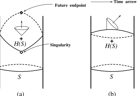
FIG. 1.: Two types of the Cauchy horizons for the spatially compact universe, in which two-spatial dimensions, $B$ factors, are suppressed.

REFERENCES

- [1] F.J.Tipler, Phys.Rev.Lett.67, 879 (1976).
- [2] F.J.Tipler, Ann.Phys.108, 1 (1977).
- [3] M.Kriele, Class.Quan.Grav.6, 1607 (1989).
- [4] K.Maeda, and A.Ishibashi, Class.Quan.Grav.11, 2569 (1996)
- [5] V.Moncrief, and D.Eardley, Gen.Rel.Grav.13, 887 (1981).
- [6] T.P.Chruściel, and A.D.Rendall, Ann.Phys.242, 349 (1995).
- [7] A.Ishibashi, T.Koike, M.Siino, and S.Kojima, Phys.Rev.D54, 7303 (1996).
- [8] V.Moncrief, and J.Isenberg, Commun.Math.Phys.89, 387 (1983).
- [9] D.A.Konkowski, and L.C.Shepley, Gen.Rel.Grav.14, 61 (1982).
- [10] C.W.Misner, and A.H.Taub, Sov.Phys.-JETP.28, 122 (1969); S.Bonanos, Commun.Math.Phys.22, 190 (1971).
- [11] S.A.Hayward, Class.Quan.Grav.10, 773 (1993).
- [12] S.W.Hawking and G.F.R.Ellis, The large scale structure of space-time, Cambridge University Press, Cambridge (1973).
- [13] B.G.Schmidt, Commun.Math.Phys.29, 49 (1972).
- [14] V.Moncrief, Phys.Rev.D23, 312 (1981); Ann.Phys.141, 83 (1982).
- [15] R.Sperb, Maximum principles and their applications, New York: Academic Press (1981).
- [16] A.Królak, J.Math.Phys.28, 2685 (1987).
- [17] P.R.Brady, and C.M.Chambers, Phys.Rev.D51, 4177 (1995).
- [18] J.K.Beem, P.E.Ehrlich, and K.L.Easley, Global Lorentzian Geometry, Pure.Appl.Math. New York: Dekker (1996),
- [19] F.J.Tipler, C.J.S Clarke, and F.G.R.Ellis, Gen.Rel.Grav. (1980).
- [20] P.R.Brady, and J.D.Smith, Phys.Rev.Lett.75, 1256 (1995).