NON-INVARIANT VELOCITY OF LIGHT AND CLOCK SYNCHRONISATION IN ACCELERATED SYSTEMS

Abstract

Clock synchronisation is conventional when inertial systems are involved. This statement is no longer true in accelerated systems. A demonstration is given in the case of a rotating platform. We conclude that theories based on the Einstein’s clock synchronisation procedure are unable to explain, for example, the Sagnac effect on the platform. Implications on very precise clock synchronisation on earth are discussed.

F. Goy - Dipartimento di Fisica - Università di Bari - Via G. Amendola, 173 - 70126 Bari - Italy - E-mail: goy@axpba1.ba.infn.it

1 Conventionality of clock synchronisation in inertial frames

Let us begin with an operationalistic definition of physical time: “time is what is measured by clocks”. If we want to apply this definition for the setting of clocks not only in one point, but everywhere in space, we see that two different and independent notions are implied:

• The rate at which time flows in each point.

• The simultaneity of events in different points of space.

Following Poincaré [3] and Einstein [4], we can use light signals for the setting of two clocks of identical fabrication, which are at two points $A$ and $B$ of an inertial frame. We send a light signal from $A$ at time $t_{1}$, which arrives at $B$ at time $t_{2}$ and comes back at $A$ at time $t_{3}$. The time $t_{2}$ of $B$ is defined to be synchronous with the midtime of departure and arrival in $A$. This definition is called the Einstein’s synchronisation. Mathematically:

$$t_{2}=t_{1}+\frac{1}{2}(t_{3}-t_{1})$$ (1.1)

Reichenbach commented [5]:”This definition is essential for the special theory of relativity, but not epistemologically necessary. If we were to follow an arbitrary rule restricted only to the form

$$t_{2}=t_{1}+\varepsilon(t_{3}-t_{1})\;\;\;\;0<\varepsilon<1$$ (1.2)

it would likewise be adequate and could not called be false. If the special theory of relativity prefers the first definition, i.e., sets $\varepsilon$ equal to $1/2$, it does so on the ground that this definition leads to simpler relations.” On the possibility to choose freely $\varepsilon$ according to (1.2) agreed, among others, Winnie [6], Grünbaum [7], Jammer [8], Mansouri and Sexl [9], Sjödin [10], Cavalleri and Bernasconi [11], Ungar [12], Vetharaniam and Stedman [13], Anderson and Stedman [14], [15]. Clearly, different values of $\varepsilon$ correspond to different values of the one way-speed of light.

A slightly different position was developed in the parametric test theory of special relativity of Mansouri and Sexl. Following these authors, we assume that there is at least one inertial frame in which light behaves isotropically. We call it the priviledged frame $\Sigma$ and denote space and time coordinates in this frame by the letters: $(x_{0},y_{0},z_{0},t_{0})$. In $\Sigma$, clocks are synchronised with Einstein’s procedure. We consider also an other system $S$ moving with uniform velocity $v<c$ along the $x_{0}$-axis in the positive direction. In $S$, the coordinates are written with lower case letters $(x,y,z,t)$. Under rather general assumptions, symmetry conditions on the two systems, the assumption that the two-way velocity of light is $c$ and furthermore that the time dilation factor has its relativistic value, one can derive the following transformation:

$$x = \frac{1}{\sqrt{1-\beta^{2}}}\left(x_{0}-vt_{0}\right)$$

$$y = y_{0}$$

$$z = z_{0}$$ (1.3)

$$t = s\left(x_{0}-vt_{0}\right)+\sqrt{1-\beta^{2}}\;\;t_{0}\;\;,$$

where $\beta=v/c$. The parameter $s$, which determines the synchronisation in the $S$ frame remains unknown. Einstein’s synchronisation in $S$ involves: $s=-v/(c^{2}\sqrt{1-\beta^{2}})$ and (1.3) becomes a Lorentz boost. For a general $s$, the inverse one-way velocity of light is given by [16]:

$$\frac{1}{c_{\rightarrow}(\Theta)}=\frac{1}{c}+\left(\frac{\beta}{c}+s\sqrt{1-\beta^{2}}\right)\cos\Theta\;\;,$$ (1.4)

where $\Theta$ is the angle between the $x$-axis and the light ray in $S$. $c_{\rightarrow}(\Theta)$ is in general dependent on the direction. A simple case is $s=0$. This means from (1.3), that at $T=0$ of $\Sigma$ we set all clocks of $S$ at $t=0$ (external synchronisation), or that we synchronise the clocks by means of light rays with velocity $c_{\rightarrow}(\Theta)=c/(1+\beta\cos\Theta)$ (internal synchronisation). It should be stressed that, unlike to the parameters of length contraction and time dilation, the parameter s cannot be tested, but its value must be assigned in accordance with the synchronisation choosen in the experimental setup. It means, as regards experimental results, that theories using different s are equivalent. Of course, they may predict different values of physical quantities (for example the one-way speed of light). This difference resides not in nature itself but in the convention used for the synchronisation of clocks. For a recent and comprehensive discussion of this subject, see [17]. A striking consequence of (1.4) is that the negative result of the Michelson-Morley experiment does not rule out an ether. Only an ether with galilean transformations is excluded, because the galilean transformations do not lead to an invariant two-way velocity of light in a moving system.

Strictly speaking, the conventionality of clock synchronisation was only shown to hold in inertial frames. The derivation of equation (1.3) is done in inertial frames and is based on the assumption that the two-way velocity of light is constant in all directions. This last assumption is no longer true in accelerated systems. But special relativity is not only used in inertial frames. A lot of textbooks bring examples of calculations done in accelerated systems, using infinitesimal Lorentz transformations. Such calculations use an additional assumption: the so-called Clock Hypothesis, which states that the rate of an accelerated ideal clock is identical to that of the instantaneously comoving inertial frame. This hypothesis first used implicitely by Einstein in his article of 1905 was superbly confirmed in the famous timedecay experiment of muons in the CERN, where the muons had an acceleration of $10^{18}g$, but where their timedecay was only due to their velocity [18]. We stress here the logical independence of this assumption from the structure of special relativity as well as from the assumptions necessary to derive (1.3). The opinion of the author is that the Clock Hypothesis, added to special relativity in order to extend it to accelerated systems leads to logical contradictions when the question of synchronisation is brought up. This idea was also expressed by Selleri [19]. The following example (see [20]) shows it: imagine that two distant clocks are screwed on an inertial frame (say a train) and synchronised with an Einstein’s synchronisation. The train accelerates during a certain time. After that, the acceleration stops and the train has again an inertial mouvement. It is easy to show that the clocks are no more Einstein’s synchronous. So the Clock Hypothesis is inconsistent with the clock setting of relativity. On the other hand, the Clock Hypothesis is tested with a high degree of accuracy [21] and cannot be rejected, so one has to reject the clock setting of special relativity. The only theory which is consistent with the Clock Hypothesis is based on transformations (1.3) with $s=0$. This is an ether theory. The fact that only an ether theory is consistent with accelerated motion give strong evidences that an ether exist, but does not involve inevitably that our velocity relative to the ether is measurable. It remains an important open question which is beyond the scope of this paper. The opinion of the author is that it cannot be measured in the above example, in spite of the logical difficulties of special relativity. There are strong evidences that when a temporary acceleration is used to go from one inertial frame to an other, an “absolute” motion cannot be measured, as it has been shown by the author in the case of stellar aberration [22]. The situation could be different when a permanent acceleration acts on a system. The logical difficulties of special relativity indicates that the relativity principle (The law of physics are the same in all inertial frames) does not only express an objective property of nature, but also a human choice about the setting of clocks. The objective part of the relativity principle is expressed in the statement: an uniform motion through the ether is not detectable. Equations (1.3) obeys to this second statement.

2 The Sagnac effect

An uniform motion through the ether was never detected, what is expressed in the negative result of the Michelson-Morley experiment. In contrary, rotational motion can be detected by mechanical methods like the Foucault pendulum as well as by luminuferous methods like in the Sagnac effect. Eight years after 1905, Sagnac wrote an article whose title shows that he thought to have proved the reality of ether [23]. The Sagnac effect is essentially the observation of the phase shift between two coherent beams travelling on opposite paths in an interferometer placed on a rotating platform. In 1925, Michelson and Gale [24], detected the earth rotation rate with a giant interferometer constructed with this aim. Michelson explained the measured effect with a velocity of light which is not constant. Nowdays the Sagnac effect is observed with light (in ring lasers and fiber optics interferometers [25]) and in interferometers built for electrons [26], neutrons [27], atoms [28] and superconducting Cooper pairs [29]. The phase shift in interferometers is a consequence of the time delay between the arrival of the two beams, so a Sagnac effect is also measured directly with atomic clocks timing light beams sent around the earth via satellites [30].

In the typical experiment for the study of the effect, a monochromatic light source placed on a disk emits two coherent light beams in opposite directions along the circumference until they reunite after a $2\pi$ propagation. The positionning of the interference figure depends on the disk rotational velocity. Textbooks deduce the Sagnac formula in the laboratory, but say nothing about the description of the phenomenon on the rotating platform. Exception to this trend are Michelson [24], Langevin [31], Anandan [32], Dieks and Nienhuis [33] and Post [34], but dissatisfaction remains widespread, because none of these treatments is free of ambiguities. Michelson uses a noninvariant velocity of light, but with a galilean addition of velocities, which is in contradiction with his experiment of 1887. Langevin, in his 1937, paper recognized the possibility of a nonstandard velocity of light on the rotating platform, but gives a formula only valid to the first order. Post’s relativistic formula is not generally valid, but limited to the case where the origin of the tangential inertial frame coincides with the center of the rotating disk.

So let us deduce here the Sagnac formula for a circular Sagnac device rotating in the anticlockwise sense in the priviledged frame $\Sigma$, for simplicity. We first calculate the time difference between a clockwise and an anticlockwise beam of light constrained to follow a circular path of radius R as seen by an observer in the laboratory and secondly we will make the calculation on the rim of the disk. The two beams leave the beamsplitter at time $t_{0}=0$ when it is in position C (see figure 1). The clockwise circulation is opposite to the direction of rotation and meets the beamsplitter when it is in position C’ shifted by $\Delta s^{\prime}$ with respect to C, at time $t_{0}^{\prime}$. The anticlockwise beam, travelling in the same direction as the direction of rotation meets the beamsplitter in the later position C”, shifted by $\Delta s^{\prime\prime}$, with respect to C at time $t_{0}^{\prime\prime}$. The geometry is given in the following figure. $\omega$ is the rate of rotation of the interferometer.

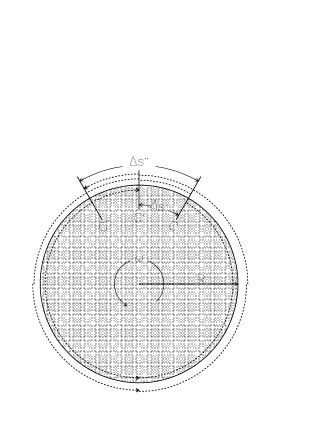
Figure 1: Simplified Sagnac configuration: the light beams are drawn with dashed lines

We have:

$$\Delta s^{\prime}=\omega Rt_{0}^{\prime}\;\;;\;\;\; L_{0}-\Delta s^{\prime}=ct_{0}^{\prime}$$ (2.1)

and

$$\Delta s^{\prime\prime}=\omega Rt_{0}^{\prime\prime}\;\;;\;\;\; L_{0}+\Delta s^{\prime\prime}=ct_{0}^{\prime\prime}\;\;,$$ (2.2)

where $L_{0}$ is the circumference of the rotating disk measured in the laboratory. The length of this circumference is reduced relative to the length $L=2\pi R$ measured directly on the disk (see section 3 for a discussion of the geometry of the rotating disk). We have: $L_{0}=L\sqrt{1-\omega^{2}R^{2}/c^{2}}$. Eliminating $\Delta s^{\prime}$ and $\Delta s^{\prime\prime}$ from equations (2.1) and (2.2), we obtain the time difference $\Delta t_{0}=t_{0}^{\prime\prime}-t_{0}^{\prime}$ in the laboratory

$$\Delta t_{0}=\frac{4\omega A}{c^{2}\sqrt{1-\omega^{2}R^{2}/c^{2}}}\;\;,$$ (2.3)

where $A$ stands for $\pi R^{2}$. Because of the time dilation, an observer on the platform must find a time difference $\Delta t$, so that:

$$\Delta t_{0}=\frac{\Delta t}{\sqrt{1-\omega^{2}R^{2}/c^{2}}}\;\;,$$ (2.4)

which gives using (2.3):

$$\Delta t=\frac{4\omega A}{c^{2}}$$ (2.5)

Let us now directly calculate the result on the platform, as done by Selleri [19]. Every infinitesimally small portion of the rim of the disk can be considered to be at rest in a comoving inertial frame tangential to the disk. The Clock Hypothesis of special relativity tells us that the rate of ideal clocks on the rim is the same as in the comoving inertial frame. Similary ideal unit measuring rods behaves in the same way on the rim and in the comoving inertial frame [35, p. 254]. For reasons of continuity, we must choose the same synchronisation on a small portion of the rim as in the tangeantial inertial frame. The one-way velocity of light is given by (1.4). The time difference between the arrival of the two light beams as calculated on the disk is given by:

$$\Delta t=t^{\prime\prime}-t^{\prime}=L\left(\frac{1}{c_{\rightarrow}(0)}-\frac{1}{c_{\rightarrow}(\pi)}\right)=\frac{4\omega A}{c^{2}}\left(1+\frac{sc^{2}\sqrt{1-\omega^{2}R^{2}/c^{2}}}{\omega R}\right)$$ (2.6)

Comparing this last formula to (2.5), we see that the only value giving a correct prediction of the Sagnac effect on the platform is $s=0$. In all other cases, the formula (2.5) is not recovered as it should be, because (2.3) is predicted by all theories having the general transformation (1.3) since they all use an Einstein’s synchronisation in the laboratory. In particular, the theory of special relativity gives $\Delta t=0$, when the value of $s$ given after (1.3) is substitued in (2.6).

Independently of the above considerations, we would draw the attention of the reader to our formula (2.3), which differs in the second order in $\omega R/c$, from the formula given by Post [34] and followers. In the same physical situation, he gives in the laboratory:

$$\Delta t_{0}^{Post}=\frac{4\omega A}{c^{2}\left(1-\omega^{2}R^{2}/c^{2}\right)}\;\;,$$ (2.7)

The discrepancy comes from the fact that Post does not take account of the Lorentz contraction of the circumference of the disk. From our point of view, this is erroneous. Unfortunately, the precision of measures of the Sagnac effect does not enable to decide between the two formulas on an experimental level, so that we have no empirical information on the physics of a relativistic rotating disk.

3 Clock synchronisation in the formalism of general relativity

The same disk as in section 2 is considered. We can obtain the metric on the disk as follow: in the inertial system the squared line element $ds^{2}$ in cartesian coordinates is:

$$ds^{2}=c^{2}dt_{0}^{2}-dx_{0}^{2}-dy_{0}^{2}-dz_{0}^{2}$$ (3.1)

In the formalism of general relativity one has a large liberty in the choice of the coordinate system useful for solving a given problem. Since we are doing physics and not only differential geometry, once given coordinates are choosen, the problem of their interpretation in terms of measurable quantities has still to be solved. In the case of the rotating disk it is simpler to use the coordinates in the right-hand side of the following transformations, as done for examples by Langevin [31] and by some textbooks [35, p. 253], [36, p. 107], [37, p. 281].

$$t_{0} = t$$

$$x_{0} = r\cos(\varphi+\omega t)$$

$$y_{0} = r\sin(\varphi+\omega t)$$ (3.2)

$$z_{0} = z$$

As stressed by Möller, in his treatment of the problem of the rotating disk, the first equation of (3.2) does not mean that we are dealing with Newtonian physics, where time dilation effects are missing, but that the coordinate $t$ is measured by a clock on the disk, that runs $1/\sqrt{1-\omega^{2}r^{2}/c^{2}}$ faster than the clocks of the laboratory, when compared at rest. Once this coordinate clock will be put on a disk rotating with angular velocity $\omega$ at radius $r$, it will have the same rate as the clocks in the laboratory, because of the time dilation. Similary the second and the third equation of (3.2) have a physical meaning, taking account of effects of longitudinal length contraction, only if the coordinate $\varphi$ is measured with tangential coordinates-rods that are $1/\sqrt{1-\omega^{2}r^{2}/c^{2}}$ longer than the measuring rods of the laboratory when compared at rest. Substituting (3.2) in (3.1) one can easily obtain:

$$ds^{2}=\left(1-\omega^{2}r^{2}/c^{2}\right)\left(cdt\right)^{2}-2\frac{\omega r^{2}}{c}d\varphi\left(cdt\right)-dr^{2}-r^{2}d\varphi^{2}-dz^{2}$$ (3.3)

Eq. (3.3) defines a metric $g_{ij}$ which is stationary, but not static. If $x^{0}=ct$, $x^{1}=r$, $x^{2}=\varphi$, $x^{3}=z$, its element are:

$$g_{00}=1-\omega^{2}r^{2}/c^{2}\;\;; g_{11}=g_{33}=-1$$

$$g_{02}=g_{20}=-\omega r^{2}/c\;\;; g_{22}=-r^{2}\;\;,$$ (3.4)

all other elements being zero. Note that the space-time described by (3.4) is flat because $R_{ijkl}(t_{0},x_{0},y_{0},z_{0})=0\Rightarrow R_{ijkl}(t,r,\varphi,z)=0\;\;[i,j,k,l=0,1,2,3]$, where $R_{ijkl}$ is the Riemann tensor. For the same reason of covariance, the metric defined in (3.4) is necessarly a solution of Einsteins equations in empty space $R_{ij}=0\;\;[i,j=0,1,2,3]$, where $R_{ij}$ is the Ricci tensor.

As is well known, in the case of a non-static space-time metric, the spatial part of the metric is not only given by the space-space coefficients of the four dimensional metric, but by:

$$dl^{2}=\left(-g_{\alpha\beta}+\frac{g_{0\alpha}g_{0\beta}}{g_{00}}\right)dx^{\alpha}dx^{\beta}=dr^{2}+dz^{2}+\frac{r^{2}d\varphi^{2}}{1-\omega^{2}r^{2}/c^{2}}\;\;,$$ (3.5)

where $0$ is the time index, and $\alpha,\beta$ represent the space indices and can take the values $1,2,3$. The right-hand-side of (3.5), with $dz=0$, is interpreted by most textbooks as the standard result, showing that the spatial part of the metric is not flat on the rotating disk. The opinion of the author is that it demonstrates exactly the contrary, namely that space is flat on the rotating disk. We have seen that the angle $\varphi$ was measured with tangeantial coordinates-rods, which, at rest, are longer than those of the laboratory, the radial measuring rods on the disk having the same rest length as those of the laboratory. If in contrary we had choosen tangential unit rods which, at rest, have the same length as the rods of the laboratory the coordinate $\varphi^{\prime}$ measured with these rods on the disk would satisfy the following equation:

$$d\varphi=d\varphi^{\prime}\sqrt{1-\omega^{2}r^{2}/c^{2}}\;\;,$$ (3.6)

so that measured with these “normal” rods (3.5) becomes:

$$dl^{2}=dr^{2}+dz^{2}+r^{2}d\varphi^{\prime 2}\;\;,$$ (3.7)

which is a flat metric in polar coordinates.

We now try to set clocks with an Einstein’s synchronisation on the disk. Generally, if we send a light signal from point $A$ with coordinates $x^{\alpha},\;\alpha=1,2,3$ to an infinitesimally near point $B$ with coordinates $x^{\alpha}+dx^{\alpha},\;\alpha=1,2,3$ and back, the coordinate time difference $dt_{1}$ ($dt_{2}$) for the “there” (back) trip is obtained by solving the equation $ds^{2}=0$. We obtain:

$$dt_{1,2}=\frac{1}{cg_{00}}\left[\mp g_{0\alpha}dx^{\alpha}+\sqrt{\left(g_{0\alpha}g_{0\beta}-g_{\alpha\beta}g_{00}\right)dx^{\alpha}dx^{\beta}}\right]=\pm\frac{\omega r^{2}d\varphi}{c^{2}\left(1-\omega^{2}r^{2}/c^{2}\right)}+\frac{dl_{AB}}{c\sqrt{1-\omega^{2}r^{2}/c^{2}}}$$ (3.8)

By definition the time $t_{A}$, at $A$, which is synchronous with the arrival time $t_{B}$ at $B$ is the midtime of departure and arrival at $A$. So, two Einstein-synchronous events are not coordinate-time-synchronous (see figure 2) and have a difference $\Delta t$ such that:

$$t_{B}=t_{A}+\Delta t=t_{A}-\frac{1}{c}\frac{g_{0\alpha}dx^{\alpha}}{g_{00}}=t_{A}+\frac{\omega r^{2}d\varphi}{c^{2}\left(1-\omega^{2}r^{2}/c^{2}\right)}$$ (3.9)

lfig2.eps

Figure 2: Illustration of equations (3.8) and (3.9). Einstein’s synchronous events $t_{A}$ and $t_{B}$ are joined with a dashed line. Coordinate-time synchronous events are joined with a doted line.

If we generalise this procedure, not only in an infinitesimal domain, but along a curve, we obtain that generally it is path dependant, because $\Delta t$ is not a total differential in $\varphi$ and $r$. As consequence, time can not be defined globally on the disk with Einstein’s procedure. This is what in fact happens on earth: if one synchronises atomic clocks all around the earth with Einstein’s procedure and comes back to the point of departure after a whole round trip, a time lag will result. This means that a clock is not synchronisable with itself, which is clearly absurd. Moreover, we will generally not obtain the same result, when synchronising clock A with clock B using two different paths. This mean also that if a clock B is synchronised with A and a clock C is synchronised with B, C will generally not be synchronised with A. Hence the physicist Ashby from Boulder has said: “Thus one discards Einstein’s synchronisation in the rotating frame”[38].

The existence of synchronisation problem is physically strange, because if the whole disk is initially at rest in the laboratory, with clocks near its rim synchronised with the Einstein’s procedure, since we are in $\Sigma$, then when the disks moves accelerates and attains a constant angular velocity, the clocks must slow their rate, but not desynchronise, for symmetry reasons, since they had at all time the same speed. From such a point of view, it is difficult to see why there should be any difficulty in defining the time on the rotating platform. In fact, we see that we can easily define a global time since the coordinate time $t$ is already global. Remembering that the coordinate time $t$ is measured with clocks that run faster than clocks at rest in $\Sigma$, we define a global time $t^{\prime}=\sqrt{1-\omega^{2}r^{2}/c^{2}}\;t$. The one-way velocity of light on the rim is now given by:

$$c_{\rightarrow}(\pm)=\frac{dl_{AB}}{dt^{\prime}_{1,2}}=\frac{dl_{AB}}{dt_{1,2}\sqrt{1-\omega^{2}r^{2}/c^{2}}}=\frac{c}{1\pm\omega r/c}\;\;,$$ (3.10)

where the last step comes from (3.5) and (3.8) with $dr=dz=0$ and $+$ ($-$) stands for the anticlockwise (clockwise) propagation of light. It means that the velocity of light in the tangential inertial frame is also equal to: $c_{\rightarrow}(\pm)=c/(1\pm\beta)$, with $\beta=\omega r/c$ , corresponding to a parameter $s=0$ of (1.4) and an angle $\Theta$ of $0$ ($\pi$). From here, the Sagnac effect can easily be calculated, in the same way as in section 2 and the result is found to be identical.

So we see that the formalism of general relativity is able to describe without contradictions the synchronisation of clocks on the rim of a rotating disk, but implies a velocity of light in the comoving inertial frame tangeantial to the rim which is noninvariant and so contradict the clock synchronisation of special relativity.

4 Conclusion

In inertial systems the synchronisation of clocks is conventional and a set of theories equivalent to special relativity, as regards experimental results, can be derived. When extended to accelerated motion, the synchronisation is no longer conventional and only the theory using $s=0$ from (1.3) is consistent with the Clock Hypothesis. This conclusion is confirmed in the case of the Sagnac effect. An elementary calculation shows that only $s=0$ enable to explain the Sagnac effect on the platform. Since one could say that accelerated motions have to be calculated with the formalism of general relativity, we have done it and shown that in this case also, only a noninvariant velocity of light enables to synchronise clocks globally on the platform. So, the clock synchronisation used in special relativity is inconsistent with the global definition of time used in general relativity. Moreover we have shown that, in our view, the geometry of the rotating platform is flat.

5 Acknowledgement

I want to thank the Physics Departement of Bari University for hospitality.

- [1]
- [2]
- [3] H. Poincaré, Mélanges, l’état actuel et l’avenir de la physique mathématique, Bull. Phys. Math. 28 (1904), 302–325.
- [4] A. Einstein, Zur Elektrodynamik bewgter Körper, Ann. Phys. 17 (1905), 891–921.
- [5] H. Reichenbach,The Philosophy of Space & Time, Dover, New-York, (1958).
- [6] J.A. Winnie, Special Relativity without One-Way Velocity Assumptions, Phil. Mag. 37 (1970), 81–99 and 223–238.
- [7] A. Grünbaum, Philosophical Problems of Space and Time, Reidel, Dodrecht (1973).
- [8] M. Jammer, Some Fundamental Problems in the Special Theory of Relativity, in: Problems in the Foudation of Physics (G. Toraldo di Francia, Ed.), North Holland, Amsterdam (1979).
- [9] R. Mansouri and R.U. Sexl, A Test Theory of Special Relativity: I. Simultaneity and Clock Synchronisation, II. First Order Test, III. Second-Order Test, Gen. Relat. Grav. 8 (1977), 497–513; 8 (1977) 515–524; 8 (1977), 809–813.
- [10] T. Sjödin, Synchronisation in Special Relativity and Related Theories, Nuovo Cim. 51B (1979), 229–245.
- [11] G. Cavalleri and C. Bernasconi, Invariance of Light Speed and Nonconservation of Simultaneity of Separate Events in Prerelativistic Physics and vice versa in Special Relativity, Nuovo Cim. 104B (1989), 545-561.
- [12] A.A. Ungar, Formalism to Deal with Reichenbach’s Special Theory of Relativity, Found. Phys. 6 (1991), 691–726.
- [13] I. Vetharaniam and G.E. Stedman, Synchronisation Conventions in Test Theories of Special Relativity, Found. Phys. Lett. 4 (1991), 275–281.
- [14] R. Anderson and G.E. Stedman, Distance and the Conventionality of Simultaneity in Special Relativity, Found. Phys. Lett. 5 (199), 199–220.
- [15] R. Anderson and G.E. Stedman, Spatial Measures in Special Relativity Do Not Empirically Determine Simultaneity Relations: A Reply to Coleman and Korté, Found. Phys. Lett. 7 (1994), 273–283.
- [16] F. Selleri, Theories Equivalent to Special Relativity, in: Frontiers of Fundamental Physics, (M. Barone and F. Selleri, Eds), 181–192, Plenum Press, New-York (1994).
- [17] I. Vetharaniam and G.E. Stedman, Significance of Precision Tests of Special Relativity, Phys. Lett. A. 183 (1993), 349–354.
- [18] J. Bailey et al., Measurement of Relativistic Time Dilatation for Positive and Negative Muons in Circular Orbits, Nature 268 (1977), 301–304.
- [19] F. Selleri, Noninvariant One-Way Velocity of Light, Found. Phys. 26 (1996), 641–664.
- [20] S.R. Mainwaring and G.E. Stedman, Accelerated Clock Principle in Special Relativity, Phys. Rev. A 47 (1993), 3611–3619.
- [21] A. M. Eisele, On the Behaviour of an Accelerated Clock, Helv. Phys. Act. 60 (1987), 1024–1037.
- [22] F. Goy, Aberration and the Question of Equivalence of Some Ether Theories to Special Relativity, Found. Phys. Lett. 9 (1996), 165–174.
- [23] G. Sagnac, L’éther lumineux démontré par l’effet du vent relatif d’éther dans un interféromètre en rotation uniforme, Comptes Rendus 157 (1913), 708–710; ibid., Sur la preuve de la réalité de l’éther lumineux par l’expérience de l’interférographe tournant, 1410–1413.
- [24] A.A Michelson and H.G. Gale, The Effect of Earth Rotation on the Velocity of Light, Astro. J. 61 (1925), 137–145.
- [25] R. Anderson, H.R. Bilger and G.E. Stedman, “Sagnac” effect: A Century of Earth Rotated Interferometers, Am. J. Phys. 62 (1994), 975–985.
- [26] H. Hasselbach and M. Nicklaus, Sagnac Experiment with Electrons: Observation of the Rotational Phase Shift of Electron Waves in Vacuum Phys. Rev. A 48 (1993), 143–151.
- [27] R. Colella, A.W. Overhauser, J.L. Staudenmann and S.A. Werner, Gravity and Inertia in Quantum Mechanics, Phys. Rev. A 21 (1980), 1419–1438.
- [28] P. Storey and C. Cohen-Tannoudji, The Feynman Path Integral Approach to Atomic Interferometry. A Tutorial, J. Phys. II France 4 (1994), 1999–2027.
- [29] D. Fargion, L. Chiatti and A. Aiello, Quantum Mach Effect by Sagnac Phase Shift on Cooper Pairs in rf-SQUID, preprint astro-ph/9606117, babbage.sissa.it (1996), 9 pages.
- [30] D.W. Allan et al., Accuracy of International Time and Frequency Comparisons Via Global Positioning System Satellites in Common-View, IEEE Trans. Instr. Meas. IM-34 (1985), 118–125; Science, Around-the-World Relativistic Sagnac Experiment 228 (1985), 69–70.
- [31] P. Langevin, Sur la théorie de la relativité et l’expérience de M. Sagnac, Comptes Rendus 173 (1921), 831–834; ibid., Sur l’expérience de Sagnac, 205 (1937), 304–306.
- [32] J. Anandan, Sagnac Effect in Relativistic and Nonrelativistic Physics, Phys. Rev. D 24 (1981), 338–346.
- [33] D. Dieks and G. Nienhuis, Relativistic Aspects of Nonrelativisic Quantum Mechanics, Am. J. Phys. 58 (1990), 650–655.
- [34] E.J. Post, Sagnac Effect, Rev. Mod. Phys. 39 (1967), 475–493.
- [35] C. Möller, The Theory of Relativity, second edition, Clarendon Press, Oxford (1972).
- [36] V. Fock, The Theory of Space Time and Gravitation, Pergamon Press, London (1959).
- [37] L. Landau and E.M. Lifschitz, The Classical Theory of Fields, Pergamon Press, London (1959).
- [38] N. Ashby, Relativity in the Future of Engineering, Proc. of the IEEE International Frequency Control Symposium (1993), 2–14.
- [39]