Non-coordinate time/velocity pairs in special relativity
Abstract
Motions with respect to one inertial (or “map”) frame are often described in terms of the coordinate time/velocity pair (or “kinematic”) of the map frame itself. Since not all observers experience time in the same way, other time/velocity pairs describe map-frame trajectories as well. Such coexisting kinematics provide alternate variables to describe acceleration. We outline a general strategy to examine these. For example, Galileo’s acceleration equations describe unidirectional relativistic motion exactly if one uses , where is map-frame position and is clock time in a chase plane moving such that . Velocity in the traveler’s kinematic, on the other hand, has dynamical and transformational properties which were lost by coordinate-velocity in the transition to Minkowski space-time. Its repeated appearance with coordinate time, when expressing relationships in simplest form, suggests complementarity between traveler and coordinate kinematic views.
pacs:
03.30.+p, 01.40.Gm, 01.55.+bI Introduction
Velocity and time, relative to a given inertial frame in special relativity, is ordinarily described with reference to the behavior of clocks at rest in the inertial frame of interest. We refer to this as the coordinate “kinematic” or time/velocity pair. Of course clocks not at rest in that reference or “map” frame will observe that the same motions, with respect to the same map, unfold in time quite differently. This paper is simply a look at the accelerated motion of a traveling object or traveler, according to the time elapsed on clocks other than those at rest in the inertial map frame with respect to which distances are being measured. Examples here involve clocks whose speed, relative to the map frame, is a function solely of the speed of the traveler, although other “non-coordinate kinematics” may be of use as well.
The most fundamental example of a non-coordinate kinematic centers about time elapsed on the clocks of the traveling object. The time used in describing map motions is thus proper time elapsed along the world line of the traveler, while velocity in the traveler-kinematic, , is the spatial component of 4-velocity with respect to the map frame. Unlike coordinate-velocity, traveler-kinematic velocity is thus proportional to momentum, and obeys elegant addition/transformation rules. In spite of its intuitive simplicity and usefulness for solving problems in the context of a single inertial frame, discussion of this quantity (also called “proper speed”) has been with two exceptions[1, 2] almost non-existent[2] in basic texts. The equations for constant proper acceleration look quite different in the traveler kinematic, although they too have been rarely discussed (except for example in the first edition of the classic text by Taylor and Wheeler[3]). Even in that case, they were not discussed as part of a time-velocity pair defined in the context of one inertial frame.
Another interesting kinematic for describing motion, with respect to a map-frame, centers about time elapsed on the clocks of a “Galilean chase plane”. For unidirectional motion, Galileo’s equations for constant acceleration exactly describe relativistic motions for our traveler in such a kinematic. Therefore, with appropriate inter-kinematic conversions in hand, Galileo’s equations may offer the simplest path to some relativistic answers! Galilean time and Galilean-kinematic velocity remain well defined in (3+1)D special relativity, with kinetic energy held equal to half mass times velocity squared. For non-unidirectional motion, however, the constant acceleration equations containing Galilean-observer time look more like elliptic integrals than like Galileo’s original equations.
Since all kinematics share common distance measures in the context of one inertial reference frame, they allow one to construct x-tv plots showing all variables in the context of that frame, including universal constant proper acceleration surfaces on which all flat space-time problems of this sort plot. The single frame character of these non-coordinate kinematics facilitates their graphical and quantitative use in pre-transform relativity as well, i.e. by students not yet ready for multiple inertial frames[4].
II Non-coordinate kinematics in general
First a word about notation. Upper case and are used for time and velocity, respectively, in an arbitrary kinematic. Lower case and have historically been used with both Galilean time, and with coordinate-time in Minkowski 4-space. Hence and are used for the latter time and velocity, to minimize confusion. The traveler-kinematic time/velocity pair is represented by the proper time elapsed along the world line of a traveler, and by spatial four-vector velocity . We have also chosen to use physical rather than dimensionless variables (albeit often arranged in dimensionless form) to make the equations useful to as wide a readership as possible.
This paper is basically about three points of view: that of the map, the traveler, and the observer. All un-primed variables refer to traveler motion, and all distances are measured in the reference inertial coordinate (,) frame. In short, everyone is talking about the traveler, and using the same map! However, traveler motion on the map is described variously: (i) from the map point of view with coordinate time and velocity , (ii) from the traveler point of view with traveler time and traveler kinematic velocity , and (iii) from the observer or “chase plane” point of view with observer-time and observer-kinematic velocity . The velocity definitions used here are summarized in Table I.
The most direct way to specify a general observer kinematic might be via the rate at which coordinate-time in the inertial map frame passes per unit time in the kinematic of interest. If we associate this observer time with physical clock time elapsed along the world line of a chase plane (primed frame) carrying the clocks of that kinematic, then this rate for a given kinematic can be written
| (1) |
Since physical values are never less than , it follows that any non-coordinate time , associated with a physical clock moving with respect to the map frame, will be passing more slowly than coordinate-time .
One can also relate this quantity to velocity in the kinematic of interest. Since and , it follows that the observer-kinematic velocity of our traveling object, with respect to the map frame, is related to coordinate-velocity by . Since with equality iff equals , any non-coordinate velocity , which describes the traveler motion with respect to a map frame using times from a physical (albeit non-coordinate) clock, will be higher than the coordinate-velocity describing that same motion.
Time/velocity pairs (kinematics) like the ones examined here may be defined by specifying as a function of the speed of the traveler (e.g. as a function of coordinate-velocity ). In this way the coordinate-kinematic itself is specified by setting to . If we set equal to or , where is the coordinate-speed of light, then the resulting kinematic is that associated with the time read by clocks moving with the traveler.
In order to determine for a Galilean observer, we explore further the relationship between and energy factor , where is total relativistic energy for our traveler, is kinetic energy, and is traveler rest mass. In particular, given the function , one can obtain from the relation
| (2) |
By inverting to get , one may then substitute this into (2) to get an expression for .
If we define the Galilean kinematic as one for which kinetic energy is , then , and hence . Then , which substituted into (2) above gives . Hence a “chase plane”, which holds its own value at in terms of for the traveler, will observe a velocity which is related to kinetic energy of , for the traveler in the reference inertial (map) frame. Note that , which means that the Galilean chase plane always moves a bit more slowly than does the traveler. One can also translate these “chase plane instructions” into coordinate-velocity terms, by replacing values above with the corresponding expression, and then solving for .
The generic observer-kinematic relationships discussed here, along with derived values for coordinate, traveler, and Galilean kinematics, are also listed in Table I. What follows is a look at the equations provided by each of these kinematics for describing map trajectories for our traveler under constant proper acceleration .
III Constant proper acceleration
The frame-invariant proper acceleration is most simply described with some definitions in 4-vector notation. If one writes the traveler 4-vector position as , then traveler 4-velocity is , and the 4-acceleration is where denotes the proper force (traveler-time derivative of traveler momentum) in the direction, and total relativistic energy, with respect to the map frame. Flat space-time dot products, formed by subtracting the sum of squares of the last three components from the square of the first component, include , , , and , where is the traveler’s proper acceleration.
With no loss of generality, let’s define as the ”direction of proper acceleration”. In other words, choose as the direction in which coordinate-velocity is changing. If the motion is not unidirectional, then there will also be a component of coordinate-velocity which is not changing. Choose the -direction as the direction of this non-changing component of coordinate-velocity, namely . Holding constant yields a second order differential equation whose solution, for times and distances measured from the “turnabout point” in the trajectory at which , is
| (3) |
where the constant . The correctness of this solution, as well as a number of intermediate quantities, can be established by substituting (3) into the defining equations above. For unidirectional motion, the solution simplifies to .
A first integral of the motion, which is independent of kinematic, is helpful for exploring intra-kinematic solutions of the constant acceleration equation. Since one thing in common to all kinematics are map frame distances and expressions for , we seek a relation between initial/final and initial/final position. This is nothing more than the work-energy theorem for constant proper acceleration, which takes the form . For the special case when times and distances are measured from the turnabout point, where and , this says that .
IV The examples
For the coordinate-kinematic case, and , so that putting from Table I above into the work-energy theorem above provides a constant acceleration equation relating to . It also yields a first order differential equation in terms of and , from which equations relating to , and to , can be obtained. The results for unidirectional motion, along with similarly obtained results for traveler and Galilean kinematics, are listed in Table II. Note in particular that the simplest result is found using the Galilean kinematic, wherein the full and familiar set of Galilean constant acceleration equations become available for the solving of relativistic acceleration problems. The usefulness of this fact depends on the availability of simple conversions between kinematics, to be discussed in the section below.
If motion is not unidirectional, the strategy above is complicated by the fact that is not , but instead is connected to through the relation , where may also be a function of . The strategy above still yields a first order equation in terms of and , with only minor resulting complication in the coordinate and traveler kinematic cases. The results of this for (3+1)D motion, in the three example kinematics, are summarized in Table III.
As you can see from the Table on (3+1)D acceleration, all 14 variables (, , , , , , , , , , , , , ) and 2 constants (, ) are simply related, except for Galilean time. We here take advantage of the fact that Galilean time is directly expressable in terms of traveler time , through the dimensionless expression
| (4) |
where is the standard elliptic integral of the second kind. The function defined above, and it’s inverse, , allows table entries involving Galilean time to be shortened considerably.
V Inter-kinematic relations
The connection between kinematics defined in the context of a single inertial frame, like the three example kinematics above, can be described graphically as well as with equations. The velocity inter-conversions can be obtained directly from Table I above. For example, velocity 1 can be used to calculate velocity 2 using . Time increments during a period of constant proper acceleration , on the other hand, are more complicated. For the example kinematics described here, they seem to be most simply expressed in terms of and a pair of initial and final velocities. For the unidirectional motion case, the simplest complete set of such inter conversions between the three example kinematics is provided in Table IV. Similar conversions for traveler and coordinate-kinematics, in the case of (3+1)D motion, are provided in Table V.
As a matter of practice when dealing with multiple time and velocity types, all defined within context of a single inertial frame, it is helpful to append the kinematic name to the time units, to avoid confusion. Thus, time in the traveler-kinematic may be measured in [traveler years], while velocities in the traveler-kinematic are measured in [light-years per traveler year]. Thus, from Table 4, a traveler-kinematic velocity of [light-year per traveler year] corresponds to a coordinate-kinematic velocity of [], where of course [] is shorthand for a [light-year per coordinate year]. This unitary value of traveler-kinematic velocity may serve as a landmark in the transition between non-relativistic and relativistic behaviors. For these reasons, we expect that a shorthand units notation for traveler-kinematic velocity, in particular for a [light-year per traveler year], may prove helpful in days ahead.
Before leaving the acceleration equations, it is worthwhile summarizing the findings, in mixed kinematic form as integrated expressions for constant proper acceleration. For unidirectional motion, or (1+1)D special relativity, we have shown that
| (5) |
where rapidity and lower case and refer to Galilean kinematic variables. In the (3+1)D case, this equation becomes
| (6) |
where , and is defined in equation (4) above.
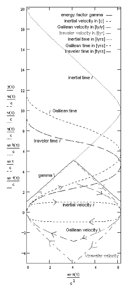
All of these velocities and times, for a given traveler with respect to a given map frame, may be plotted as trajectories over the x,y coordinate field. If we divide velocities by and times by , they can all be plotted on the same graph! For unidirectional motion, this allows us (for example) to plot all of these parameters as a function of position even if the acceleration changes, as in the 4-segment twin adventure illustrated in Figure 1.
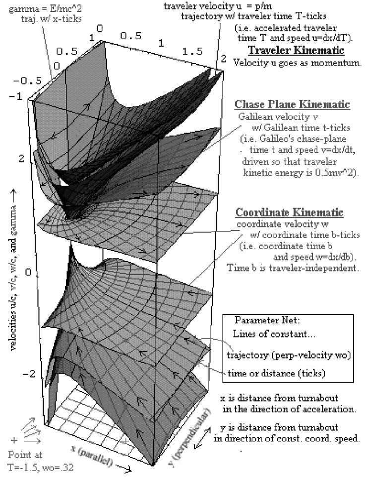
If we further divide distances in the x,y coordinate field by , and restrict trajectories to those involving a single constant acceleration trajectory, or to a family of such trajectories in (3+1)D, a single universal acceleration plot in the velocity range of interest can be assembled, on which all constant acceleration problems plot! A plot of this sort, of the three example kinematic velocities and gamma, over the linear velocity range from 0 to 3 [light-years per traveler year], is provided in Figure 2. Here the various velocity surfaces have been parameterized using equal time increments in the kinematic of the velocity being plotted, as well as with equally-spaced values of the constant transverse coordinate-velocity . It is thus easy to see that coordinate time during constant acceleration passes more quickly, as a function of position, than do either of the two kinematic times, as predicted more generally by equation (1).
All of the foregoing has been done in the context of a single inertial frame. The transformation properties of these various times and velocities between frames also deserve mention. As is well known, and apparent from the section on 4-vector acceleration above, coordinate-time is the time component of the coordinate 4-vector, while traveler-kinematic velocity provides spatial components for the velocity 4-vector. Coordinate-velocity enjoys no such role, and its comparatively messy behaviors when transforming between frames need no further introduction.
A similar inelegance is found in the well-known rule of velocity addition for coordinate-velocities. A comprehensive look at addition rules for the velocities used here, and for as well, shows that the simplest of all (to this author at least) is the rule for the relative traveler-kinematic velocity associated with particles A and B on a collision course, namely . Recall that within a single frame, . Hence on addition, the factors of traveler-kinematic velocity multiply, while the coordinate-velocity factors add.
VI Discussion
The coordinate-kinematic has been used almost exclusively in the special relativity literature to date. This is in part because the traveler-independent nature of time in a world of Galilean transforms finds its strongest (if still weak) natural analog in the coordinate-kinematic of Minkowski space-time. However, other features of velocity and time abandon the coordinate-kinematic, when the transition from Galilean to Lorentz transforms is made.
For example, we lose the second time derivative of coordinate position as a useful acceleration, and thus the coordinate kinematic loses Galileo’s equations for constant acceleration. These equations remain intact for unidirectional motion if we put our clocks into a Galilean chase plane. The role of this kinematic, in allowing proper acceleration to be written as a second time derivative of position (i.e. for which ), is illuminated by noting that unidirectional motion from rest is described by . Hence , but and are in different kinematics. If we want for time/velocity in one kinematic, a obeying is required. One can rewrite the right side of this equation as times , or as if and only if . Thus Galilean velocity is the only way to make proper acceleration a second time derivative in (1+1)D. From similarities between and the expression above for , it is easy to see why the Galilean kinematic provides an excellent low-velocity (small-argument) approximation to traveler velocity and coordinate time.
On a deeper note, the inertial nature of velocity in Galilean space-time (i.e. its proportionality to momentum), as well as its relatively elegant transformation properties, do not belong to coordinate velocity in Minkowski space-time. Velocity in the traveler kinematic inherits them instead. The traveler-kinematic also has relatively simple equations for constant acceleration. However, constant acceleration is most simply expressed in mixed-kinematic terms, using the coordinate-time derivative of a traveler-kinematic velocity component.
Thus we have a choice, to cast expressions which involve velocity in terms of either the coordinate-time derivative of position (), or in terms of the dynamically and transformationally more robust traveler-time derivative of position (). Some of the connections discussed here might be more clearly reflected than they are at present in the language that we use, had historical strategies taken the alternate path.
Acknowledgements.
This work has benefited directly from support by UM-St.Louis, and indirectly from support by the U.S. Department of Energy, the Missouri Research Board, as well as Monsanto and MEMC Electronic Materials Companies. Thanks also to family, friends, and colleagues at all stages in their careers, for their thoughts and patience concerning this “little project on the side”.REFERENCES
- [1] Sears and Brehme, Introduction to the Theory of Relativity (Addison Wesley, 1968).
- [2] W. A. Shurcliff, Special Relativity: The Central Ideas (19 Appleton St., Cambridge MA 02138, 1996).
- [3] F. Taylor and J. A. Wheeler, Spacetime Physics (W. H. Freeman, San Francisco, 1963 and 1992).
- [4] P. Fraundorf, Pre-Transform Relativity (unpublished, cf. related materials at http://www.umsl.edu/~fraundor/a1toc, 1996).
| kinematic: | generic , | coordinate , | traveler , | Galilean , |
|---|---|---|---|---|
| velocity of traveler | ||||
| {given} | ||||
| {invert } | ||||
| kinematic: | coordinate | traveler | Galilean |
|---|---|---|---|
| speed | |||
| distance | |||
| time |
| kinematic: | coordinate | traveler | Galilean |
|---|---|---|---|
| or | |||
| speed | |||
| x-velocity | |||
| y-velocity | { given, constant} | ||
| distance | |||
| distance | |||
| time |
| FromTo | energy factor | initial/final speed | (1+1)D elapsed time |
|---|---|---|---|
| GalileanTraveler | |||
| TravelerCoord. | |||
| Coord.Galilean |
| FromTo | initial/final | initial/final | (3+1)D elapsed time |
|---|---|---|---|
| GalileanTraveler | |||
| TravelerCoord. | {given, as } | ||
| Coord.Galilean |