Abstract

In a previous paper, a bound on the negative energy density seen by an arbitrary inertial observer was derived for the free massless, quantized scalar field in four-dimensional Minkowski spacetime. This constraint has the form of an uncertainty principle-type limitation on the magnitude and duration of the negative energy density. That result was obtained after a somewhat complicated analysis. The goal of the current paper is to present a much simpler method for obtaining such constraints. Similar “quantum inequality” bounds on negative energy density are derived for the electromagnetic field, and for the massive scalar field in both two and four-dimensional Minkowski spacetime.

1 Introduction

In quantum field theory, unlike in classical physics, the energy density may be unboundedly negative at a spacetime point. Such situations entail violations of all the known classical pointwise energy conditions, such as the weak energy condition [1]. This fact has been known for quite sometime [2]. Specific examples include the Casimir effect [3, 4] and squeezed states of light [5], both of which have observational support. The theoretical prediction of black hole evaporation [6] also involves negative energy densities and fluxes in a crucial way. On the other hand, if the laws of quantum field theory place no restrictions on negative energy, then it might be possible to produce gross macroscopic effects such as: violation of the second law of thermodynamics [7, 8] or of cosmic censorship [9, 10], traversable wormholes [11, 12], “warp drive”[13], and possibly time machines [12, 14]. As a result, much effort has been recently directed toward determining what constraints, if any, the laws of quantum field theory place on negative energy density. One approach involves so-called “averaged energy conditions” (see, for example, [15]-[19]), i.e., averaging the local energy conditions over timelike or null geodesics. Another method employs “quantum inequalities” (QI’s) [7, 20], which are constraints on the magnitude and duration of negative energy fluxes and densities. The current paper is another in a series which is exploring the ramifications of this approach [21]-[25]. (For a more comprehensive discussion of the history of these topics, see the introductions of Refs.[21, 22] and the references therein.)

The QI’s have the general form of an inverse relation between an integral involving the the energy density or flux over a finite time interval and a power of that interval. More precise forms of the inequality were originally derived for negative energy fluxes [20], and later for negative energy density [21, 22]. This form of QI’s involves “folding” the stress energy tensor into a “sampling function”, i.e., a peaked function of time whose time integral is unity. For example, it was shown in Ref.[21] that for the free quantized massless scalar field in four-dimensional Minkowski spacetime,

$$\hat{\rho}\equiv{t_{0}\over\pi}\,\int_{-\infty}^{\infty}\,{{\langle T_{00}\rangle\,dt}\over{t^{2}+t_{0}^{2}}}\,\geq-{3\over{32{\pi}^{2}}{t_{0}}^{4}}\,,$$ (1)

for all choices of the sampling time, $t_{0}$. Here $\langle T_{00}\rangle$ is the renormalized expectation value of the energy density evaluated in an arbitrary quantum state $|\psi\rangle$, in the frame of an arbitrary inertial observer whose proper time coordinate is $t_{0}$. The physical implication of this QI is that such an observer cannot see unboundedly large negative energy densities which persist for arbitrarily long periods of time. The QI constraints can be considered to be midway between the local energy conditions, which are applied at a single spacetime point, and the averaged energy conditions which are global, in the sense that they involve averaging over complete or half-complete geodesics. The QI’s place bounds on the magnitude and duration of the negative energy density in a finite neighborhood of a spacetime point along an observer’s worldline.

These inequalities were derived for Minkowski spacetime, in the absence of boundaries. However, we recently argued [23] that if one is willing to restrict the choice of sampling time, then the bound should also hold in curved spacetime and/or one with boundaries . For example, we proved that the inequality Eq. (1) holds in the case of the Casimir effect for sampling times much smaller than the distance between the plates. It turns out that this observation has some interesting implications for traversable wormholes [23]. Quantum inequalities in particular curved spacetimes, which reduce to Eq. (1) in the short sampling time limit, are given in Ref. [24].

In the original derivation of Eq. (1), we used a rather cumbersome expansion of the mode functions of the quantum field in terms of spherical waves. The goal of the present paper is to present a much more transparent derivation of QI bounds, based on a plane wave mode expansion. In so doing, we prove new QI constraints on negative energy density for the quantized electromagnetic and massive scalar fields. In Sec. 2, we derive a QI bound for the massive scalar field in both four and two-dimensional Minkowski spacetime. Our earlier result, Eq. (1), is recovered as a special case when the mass $m$ goes to zero. A similar bound is obtained for the electromagnetic field in Sec. 3. Our results, and their implications for the existence of traversable wormholes, are discussed in Sec. 4. Our metric sign convention is $(-,+,+,+)$.

2 The Massive Scalar Field

2.1 Four-Dimensions

In this section we derive a QI-bound on the energy density of a quantized uncharged massive scalar field in four-dimensional flat spacetime. The wave equation for the field is

$$(\Box-m^{2})\phi=0\,,$$ (2)

where $\Box\equiv\eta^{\mu\nu}\,\partial_{\mu}\partial_{\nu}$. We can expand the field operator in terms of creation and annihilation operators as

$$\phi=\sum_{\bf k}({a_{\bf k}}{f_{\bf k}}+a^{\dagger}_{\bf k}{f_{\bf k}}^{\ast}).$$ (3)

Here the mode functions are taken to be

$$f_{\bf k}={i\over\sqrt{2\omega V}}e^{i({\bf k\cdot x}-\omega t)},$$ (4)

where

$$\omega=\sqrt{{|{\bf k}|}^{2}+m^{2}}\,,$$ (5)

$m$ is the rest mass, and $V$ is the normalization volume. The stress tensor for the massive scalar field is

$$T_{\mu\nu}=\phi_{,\mu}\phi_{,\nu}-{1\over 2}{\eta_{\mu\nu}(\phi_{,\alpha}\phi^{,\alpha}+m^{2}\,{\phi}^{2})}\,.$$ (6)

The renormalized expectation value of the energy density, in an arbitrary quantum state $|\psi\rangle$, is

$$\langle T_{00}\rangle = {{\rm Re}\over{2V}}{\sum_{\bf k^{\prime},k}}{{(\omega^{\prime}\omega+{\bf k^{\prime}\cdot k})}\over{\sqrt{\omega^{\prime}\omega}}}\,\left[\langle a^{\dagger}_{\bf k^{\prime}}{a_{\bf k}}\rangle\,e^{i(\omega^{\prime}-\omega)t}+\langle{a_{\bf k^{\prime}}}{a_{\bf k}}\rangle\,e^{-i(\omega^{\prime}+\omega)t}\right]$$ (7)

$$+ {{\rm Re}\over{2V}}{\sum_{\bf k^{\prime},k}}{{m^{2}}\over{\sqrt{\omega^{\prime}\omega}}}\,\left[\langle a^{\dagger}_{\bf k^{\prime}}{a_{\bf k}}\rangle\,e^{i(\omega^{\prime}-\omega)t}-\langle{a_{\bf k^{\prime}}}{a_{\bf k}}\rangle\,e^{-i(\omega^{\prime}+\omega)t}\right]\,.$$

Here the energy density is evaluated in the reference frame of an inertial observer, at an arbitrary spatial point which we choose to be ${\bf x}=0$. The time coordinate $t$ is the proper time of this observer. Because of the underlying Lorentz invariance of the field theory, we may of course choose the frame of any inertial observer in Minkowski spacetime.

Following Refs. [20, 21], we multiply $\langle T_{00}\rangle$ by a peaked function of time whose time integral is unity and whose characteristic width is $t_{0}$. A convenient choice of such a function is $t_{0}/[\pi(t^{2}+t_{0}^{2})]$. Define the integrated energy density to be

$$\hat{\rho}\equiv{t_{0}\over\pi}\,\int_{-\infty}^{\infty}\,{{\langle T_{00}\rangle\,dt}\over{t^{2}+t_{0}^{2}}}\,.$$ (8)

Substitution of Eq. (7) into Eq. (8) and performance of the integration yields

$$\hat{\rho} = {{\rm Re}\over{2V}}{\sum_{\bf k^{\prime},k}}{{(\omega^{\prime}\omega+{\bf k^{\prime}\cdot k})}\over{\sqrt{\omega^{\prime}\omega}}}\,\left[\langle a^{\dagger}_{\bf k^{\prime}}{a_{\bf k}}\rangle\,e^{-|\omega^{\prime}-\omega|t_{0}}+\langle{a_{\bf k^{\prime}}}{a_{\bf k}}\rangle\,e^{-(\omega^{\prime}+\omega)t_{0}}\right]$$ (9)

$$+ {{\rm Re}\over{2V}}{\sum_{\bf k^{\prime},k}}{{m^{2}}\over{\sqrt{\omega^{\prime}\omega}}}\,\left[\langle a^{\dagger}_{\bf k^{\prime}}{a_{\bf k}}\rangle\,e^{-|\omega^{\prime}-\omega|t_{0}}-\langle{a_{\bf k^{\prime}}}{a_{\bf k}}\rangle\,e^{-(\omega^{\prime}+\omega)t_{0}}\right]\,.$$

Now write ${\bf k^{\prime}\cdot k}=k^{\prime}_{x}k_{x}+k^{\prime}_{y}k_{y}+k^{\prime}_{z}k_{z}$, and apply the lemma in Appendix B to each of the sums in Eq. (9), e.g.,

$${\sum_{\bf k^{\prime},k}}{{k^{\prime}_{x}k_{x}}\over{\sqrt{\omega^{\prime}\omega}}}\,\langle a^{\dagger}_{\bf k^{\prime}}{a_{\bf k}}\rangle\,e^{-|\omega^{\prime}-\omega|t_{0}}\geq{\sum_{\bf k^{\prime},k}}{{k^{\prime}_{x}k_{x}}\over{\sqrt{\omega^{\prime}\omega}}}\,\langle a^{\dagger}_{\bf k^{\prime}}{a_{\bf k}}\rangle\,e^{-(\omega^{\prime}+\omega)t_{0}}\,.$$ (10)

We then obtain

$$\hat{\rho} \geq {{\rm Re}\over{2V}}{\sum_{\bf k^{\prime},k}}{{(\omega^{\prime}\omega+{\bf k^{\prime}\cdot k})}\over{\sqrt{\omega^{\prime}\omega}}}\,e^{-(\omega^{\prime}+\omega)t_{0}}\,\left[\langle a^{\dagger}_{\bf k^{\prime}}{a_{\bf k}}\rangle\,+\langle{a_{\bf k^{\prime}}}{a_{\bf k}}\rangle\right]$$ (11)

$$+ {{\rm Re}\over{2V}}{\sum_{\bf k^{\prime},k}}{{m^{2}}\over{\sqrt{\omega^{\prime}\omega}}}\,e^{-(\omega^{\prime}+\omega)t_{0}}\,\left[\langle a^{\dagger}_{\bf k^{\prime}}{a_{\bf k}}\rangle\,-\langle{a_{\bf k^{\prime}}}{a_{\bf k}}\rangle\,\right]\,.$$

For the first sum (i.e., the one involving $\omega^{\prime}\omega$), apply the first lemma in Appendix A, where we take $h_{j}=(1/2)(\sqrt{\omega/V})\,e^{-\omega t_{0}}$. Apply the same lemma to each term in the sum which involves ${\bf k^{\prime}\cdot k}$, taking $h_{j}=(k_{i}/{2\sqrt{\omega V}})\,e^{-\omega t_{0}}$, with $i=x,y,z$. For the last sum, involving $m^{2}$, use the second lemma in Appendix A choosing $h_{j}=(m/{2\sqrt{\omega V}})\,e^{-\omega t_{0}}$. The result is

$$\hat{\rho}\geq-{1\over{2V}}\,\sum_{\bf k}\,\omega e^{-2\omega t_{0}}\,,$$ (12)

where we have used $|{{\bf k}|}^{2}={\omega}^{2}-m^{2}$. Now let $V\rightarrow\infty$, in which limit $\sum_{\bf k}\rightarrow(V/8{\pi}^{3})\,\int_{-\infty}^{\infty}d^{3}k$. Performing the angular integrations and changing variables we get

$$\hat{\rho}\geq-{1\over{4{\pi}^{2}}}\int_{m}^{\infty}d\omega\sqrt{{\omega}^{2}-m^{2}}\,{\omega}^{2}\,e^{-2\omega t_{0}}\,.$$ (13)

Let $x\equiv 2\omega t_{0},\,y\equiv 2mt_{0}$. We may then rewrite the integral in Eq. (13) as

$$\hat{\rho}\geq-{1\over{64{\pi}^{2}}{t_{0}}^{4}}\int_{y}^{\infty}dx\,\sqrt{x^{2}-y^{2}}\,x^{2}\,e^{-x}\,.$$ (14)

If we now let

$$G(y)\equiv{1\over 6}\int_{y}^{\infty}dx\,\sqrt{x^{2}-y^{2}}\,x^{2}\,e^{-x}\,,$$ (15)

then our QI-bound may be written as

$$\hat{\rho}\geq-{3\over{32{\pi}^{2}}{t_{0}}^{4}}\,G(y)\,,$$ (16)

for all $t_{0}$. A plot of $G(y)$ versus $y$ is given in Fig. 1.

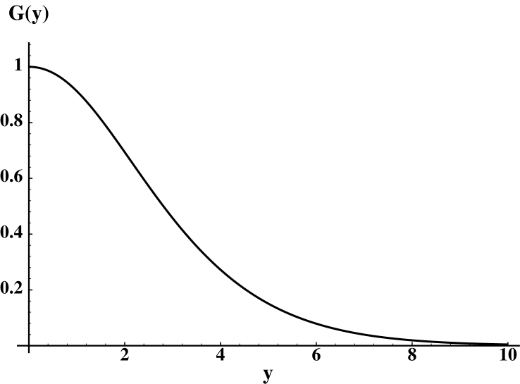
Figure 1:

The graph of $G(y)$ versus $y$.

We see that as $m\rightarrow 0$ (for fixed $t_{0}$), $y\rightarrow 0$ and $G(y)\rightarrow 1$, hence in this case our bound reduces to

$$\hat{\rho}\geq-{3\over{32{\pi}^{2}}{t_{0}}^{4}}\,,$$ (17)

for all $t_{0}$, which is the QI for the massless scalar field - originally obtained in [21] by a much more complicated method. As $m\rightarrow\infty$ (for fixed $t_{0}$), $y\rightarrow\infty$, and we see from the graph that $G(y)\rightarrow 0$. Note that our bound becomes more stringent as $m$ increases, and hence it becomes increasingly difficult to produce large negative energy densities. This result is not surprising, since now one has to overcome the positive rest mass energy of the field quanta. For $t_{0}\gg 1/m$ (with fixed $m$), corresponding to sampling times much larger than the Compton wavelength of the particle, we also have $y\rightarrow\infty$ and $G(y)\rightarrow 0$. Note that, due to the factor of $G(y)$, the right-hand side of Eq. (16) vanishes more rapidly than the right-hand side of Eq. (17) in the $t_{0}\rightarrow\infty$ limit. This can be interpreted as showing that negative energy due to a massive scalar field must be more highly localized than that due to a massless field.

2.2 Two-Dimensions

The derivation of a QI bound on the energy density of a massive scalar field in two-dimensional spacetime is very similar to the discussion given in the previous section for the four-dimensional case. One follows the same steps as in that treatment, but replacing the normalization volume $V$ with a periodicity length $L$, and ${\bf k}$ and ${\bf x}$ by $k$ and $x$, respectively. This procedure yields

$$\hat{\rho}\geq-{1\over{2L}}\,\sum_{k}\,\omega e^{-2\omega t_{0}}\,,$$ (18)

where we have used $k^{2}={\omega}^{2}-m^{2}$. It is at this stage that the 2D analysis differs from the 4D case. Now let $L\rightarrow\infty$, in which limit $\sum_{k}\rightarrow(L/{2\pi})\,\int_{-\infty}^{\infty}dk$. Rewriting the integral in terms of $\omega$, one obtains

$$\hat{\rho}\geq-{1\over{2\pi}}\int_{m}^{\infty}\,{{{\omega}^{2}\,e^{-2\omega t_{0}}}\over\sqrt{{\omega}^{2}-m^{2}}}\,d\omega\,.$$ (19)

Let

$$I\equiv\int_{m}^{\infty}\,{{{\omega}^{2}\,e^{-2\omega t_{0}}}\over\sqrt{{\omega}^{2}-m^{2}}}\,d\omega\,.$$ (20)

This expression can be rewritten [26] in terms of modified Bessel functions of the second kind, $K_{\nu}(y)$, as follows

$$I=-m^{2}\,K^{\prime}_{1}(2mt_{0})\,,$$ (21)

where the prime denotes differentiation with respect to the argument. We now employ the relation [27]

$$K^{\prime}_{1}(y)=-{1\over 2}\,[K_{0}(y)+K_{2}(y)]\,,$$ (22)

where again $y\equiv 2mt_{0}$. The integral $I$ can then be written as

$$I = {1\over{8{t_{0}}^{2}}}\,y^{2}\,[K_{0}(y)+K_{2}(y)]$$ (23)

$$= {1\over{4{t_{0}}^{2}}}\,F(y)\,.$$

Thus our QI-bound may be written as

$$\hat{\rho}\geq-{1\over{8\pi{t_{0}}^{2}}}\,F(y)\,,$$ (24)

for all $t_{0}$. The function $F(y)$ is plotted against $y$ in Fig. 2.

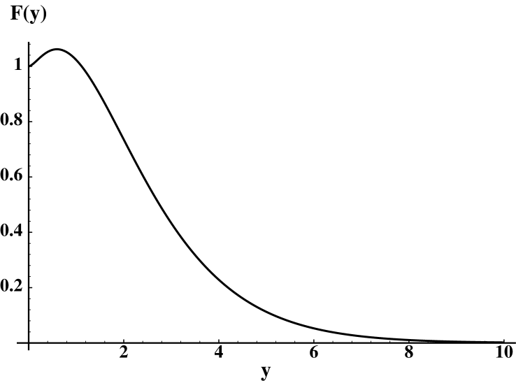
Figure 2:

The graph of $F(y)$ versus $y$.

As $m\rightarrow 0$ (for fixed $t_{0}$), $F(y)\rightarrow 1$, and our inequality becomes

$$\hat{\rho}\geq-{1\over{8\pi{t_{0}}^{2}}}\,,$$ (25)

for all $t_{0}$, which is the QI for the massless scalar field in 2D [21]. For large $y$, the behavior of the graph is qualitatively similar to the 4D case. However, for $y$ in the approximate range $0\leq y\leq 1.2$, there appears to be a small peak in the value of $F(y)$. In the case of flat spacetime, this seems to be an artifact of 2D, since no corresponding peak occurs in the 4D case [28]. Rather than indicating that one could actually supercede the $m=0$ bound in the 2D massive case for certain values of $y$, this result may perhaps imply that the bound given in Eq. (24) is not optimal over this range. In either case, the relative height of the peak above the value of $F(y)=1$ (corresponding to the massless case) is too small to produce a dramatic change in the QI bound. As we argued in Ref.[23], the constant on the right-hand side of the inequality would typically have to be larger by many orders of magnitude to result in large macroscopic effects.

3 The Electromagnetic Field

In this section, we derive a QI-bound for the energy density of the free quantized electromagnetic field in 4D Minkowski spacetime. The absence of source charges and the imposition of the Coulomb gauge condition imply

$$A^{0}=\Phi=0\,,$$

$${\bf\nabla\cdot A}=0\,,$$ (26)

where ${\bf A}$ is the vector potential, and $\Phi$ is the scalar potential. The wave equation is

$${\bf\Box A}=0\,.$$ (27)

The vector potential can be expanded in terms of creation and annihilation operators as

$${\bf A}({\bf x},t)=\sum_{{\bf k}\lambda}({a_{{\bf k}\lambda}}\hat{e}_{{\bf k}\lambda}{f_{\bf k}}+a^{\dagger}_{{\bf k}\lambda}\hat{e}_{{\bf k}\lambda}{f_{\bf k}}^{\ast})\,,$$ (28)

where the $\hat{e}_{{\bf k}\lambda}$ are unit linear polarization vectors and thus $\lambda=1,2$. Here the sum $\sum_{{\bf k}\lambda}=\sum_{\bf k}\,\sum_{\lambda}$. The mode functions $f_{\bf k}$ are again given by

$$f_{\bf k}={i\over\sqrt{2\omega V}}e^{i({\bf k\cdot x}-\omega t)},$$ (29)

i.e., we assume periodic boundary conditions in a box with normalization volume $V$. We will adopt the convention that one of the polarization vectors changes direction as ${\bf k}\rightarrow-{\bf k}$, but the other does not. That is, we have

$$\hat{e}_{{\bf k}1}{\bf\times}\hat{e}_{{\bf k}2} = {\bf{\hat{k}}}\,,$$

$$\hat{e}_{-{\bf k}1} = -\hat{e}_{{\bf k}1}\,,$$

$$\hat{e}_{-{\bf k}2} = \hat{e}_{{\bf k}2}\,,$$ (30)

so that $\hat{e}_{-{\bf k}1}{\bf\times}\hat{e}_{-{\bf k}2}=-{\bf{\hat{k}}}$. The commutation relations for the creation and annihilation operators are

$$\quad\qquad[a_{{\bf k}\lambda},a^{\dagger}_{{\bf k^{\prime}}\lambda^{\prime}}]=\delta_{{\bf k}{\bf k^{\prime}}}\,\delta_{\lambda\lambda^{\prime}}\,,$$ (31)

$$[a_{{\bf k}\lambda},a_{{\bf k^{\prime}}\lambda^{\prime}}]=0\,,$$ (32)

$$[a^{\dagger}_{{\bf k}\lambda},a^{\dagger}_{{\bf k^{\prime}}\lambda^{\prime}}]=0\,.$$ (33)

With the gauge choice made in Eq. (26), the electric field operator becomes

$${\bf E}=-\dot{\bf A}=\sum_{{\bf k}\lambda}\,i\omega\,({a_{{\bf k}\lambda}}\hat{e}_{{\bf k}\lambda}{f_{\bf k}}-a^{\dagger}_{{\bf k}\lambda}\hat{e}_{{\bf k}\lambda}{f_{\bf k}}^{\ast})\,.$$ (34)

Similarly the magnetic field operator is given by

$${\bf B}={\bf\nabla\times A}=\sum_{{\bf k}\lambda}\,i\omega\,({a_{{\bf k}\lambda}}\hat{b}_{{\bf k}\lambda}{f_{\bf k}}-a^{\dagger}_{{\bf k}\lambda}\hat{b}_{{\bf k}\lambda}{f_{\bf k}}^{\ast})\,.$$ (35)

Here we define

$$\hat{b}_{{\bf k}\lambda}={\bf\hat{k}}{\bf\times}\hat{e}_{{\bf k}\lambda}\,,$$ (36)

so that

$$\hat{b}_{{\bf k}1}={\bf{\hat{k}}}{\bf\times}\hat{e}_{{\bf k}1}=\hat{e}_{{\bf k}2}\,,$$ (37)

$$\quad\hat{b}_{{\bf k}2}={\bf{\hat{k}}}{\bf\times}\hat{e}_{{\bf k}2}=-\hat{e}_{{\bf k}1}\,,$$ (38)

and therefore

$$\hat{b}_{-{\bf k}1}=-{\bf{\hat{k}}}{\bf\times}\hat{e}_{-{\bf k}1}=\hat{e}_{{\bf k}2}=\hat{b}_{{\bf k}1}\,,$$ (39)

and

$$\quad\hat{b}_{-{\bf k}2}=-{\bf{\hat{k}}}{\bf\times}\hat{e}_{-{\bf k}2}=\hat{e}_{{\bf k}1}=-\hat{b}_{{\bf k}2}\,.$$ (40)

The stress energy tensor for the electromagnetic field is

$$T_{00}={1\over 2}(E^{2}+B^{2})\,.$$ (41)

If we compute the renormalized expectation value $\langle T_{00}\rangle$, in an arbitrary quantum state $|\psi\rangle$, evaluated at ${\bf x}=0$, and fold this into our sampling function we obtain

$$\hat{\rho} \equiv {t_{0}\over\pi}\,\int_{-\infty}^{\infty}\,{{\langle T_{00}\rangle\,dt}\over{t^{2}+t_{0}^{2}}}$$ (42)

$$= {{\rm Re}\over{2V}}\sum_{{\bf k,k^{\prime}}\atop{\lambda,\lambda^{\prime}}}\sqrt{\omega^{\prime}\omega}\,[(\hat{e}_{{\bf k}\lambda}\cdot\hat{e}_{{\bf k^{\prime}}\lambda^{\prime}})\,+\,(\hat{b}_{{\bf k}\lambda}\cdot\hat{b}_{{\bf k^{\prime}}\lambda^{\prime}})]\,$$

$$\times\left[\langle a^{\dagger}_{{\bf k}\lambda}{a_{{\bf k^{\prime}}\lambda^{\prime}}}\rangle\,e^{-|\omega-\omega^{\prime}|t_{0}}+\langle{a_{{\bf k}\lambda}}{a_{{\bf k^{\prime}}\lambda^{\prime}}}\rangle\,e^{-(\omega+\omega^{\prime})t_{0}}\right]\,.$$

Now write $\hat{e}_{{\bf k}\lambda}\cdot\hat{e}_{{\bf k^{\prime}}\lambda^{\prime}}={({\hat{e}}_{{\bf k}\lambda})}_{x}\,{({\hat{e}}_{{\bf k^{\prime}}\lambda^{\prime}})}_{x}\,+\,{({\hat{e}}_{{\bf k}\lambda})}_{y}\,{({\hat{e}}_{{\bf k^{\prime}}\lambda^{\prime}})}_{y}\,+\,{({\hat{e}}_{{\bf k}\lambda})}_{z}\,{({\hat{e}}_{{\bf k^{\prime}}\lambda^{\prime}})}_{z}$, and similarly for the dot product involving the $\hat{b}$ vectors. Expanding Eq. (42) in this fashion, one gets six terms. To each of these terms we apply the lemma in Appendix B, e.g.,

$$\!\!\!\!\!\!\!\!\!\sum_{{\bf k,k^{\prime}}\atop{\lambda,\lambda^{\prime}}}\,\sqrt{\omega\omega^{\prime}}\,{({\hat{e}}_{{\bf k}\lambda})}_{x}\,{({\hat{e}}_{{\bf k^{\prime}}\lambda^{\prime}})}_{x}\,{\langle a^{\dagger}_{{\bf k}\lambda}{a}_{{\bf k^{\prime}}\lambda^{\prime}}\rangle}\,e^{-{|\omega-\omega^{\prime}|}t_{0}}$$

$$\!\!\!\!\!\!\!\geq\sum_{{\bf k,k^{\prime}}\atop{\lambda,\lambda^{\prime}}}\,\sqrt{\omega\omega^{\prime}}\,{({\hat{e}}_{{\bf k}\lambda})}_{x}\,{({\hat{e}}_{{\bf k^{\prime}}\lambda^{\prime}})}_{x}\,{\langle a^{\dagger}_{{\bf k}\lambda}\,{a}_{{\bf k^{\prime}}\lambda^{\prime}}\rangle}\,e^{-(\omega+\omega^{\prime})t_{0}}\,.$$ (43)

Recombining the terms, we then obtain

$$\hat{\rho}\!\! \geq \!\!{{\rm Re}\over{2V}}\sum_{{\bf k,k^{\prime}}\atop{\lambda,\lambda^{\prime}}}\sqrt{\omega^{\prime}\omega}\,[(\hat{e}_{{\bf k}\lambda}\cdot\hat{e}_{{\bf k^{\prime}}\lambda^{\prime}})\,+\,(\hat{b}_{{\bf k}\lambda}\cdot\hat{b}_{{\bf k^{\prime}}\lambda^{\prime}})]\,$$ (44)

$$\times\left[\langle a^{\dagger}_{{\bf k}\lambda}{a_{{\bf k^{\prime}}\lambda^{\prime}}}\rangle\,+\langle{a_{{\bf k}\lambda}}{a_{{\bf k^{\prime}}\lambda^{\prime}}}\rangle\right]\,e^{-(\omega+\omega^{\prime})t_{0}}\,.$$

An analogous separation of the dot products in Eq. (44) into components, repeated application of the first lemma in Appendix A, and a recombination of terms results in

$$\hat{\rho}\geq-{1\over{2V}}\,\sum_{{\bf k}\lambda}\,\omega e^{-2\omega t_{0}}\,,$$ (45)

where we have used $h_{j}=(1/2)\,{({\hat{e}}_{{\bf k}\lambda})}_{i}\,\times\,\sqrt{\omega/V}\,e^{-\omega t_{0}}$ and $h_{j}=(1/2)\,{({\hat{b}}_{{\bf k}\lambda})}_{i}\,\times\sqrt{\omega/V}\,e^{-\omega t_{0}}$, with $i=x,y,z$. Evaluation of the sum over $\lambda$ gives

$$\hat{\rho}\geq-{1\over V}\,\sum_{\bf k}\,\omega e^{-2\omega t_{0}}\,.$$ (46)

Now let $V\rightarrow\infty$, so

$$\hat{\rho}\geq-{1\over{2{\pi}^{2}}}\,\int_{0}^{\infty}\,d{\omega}\,{\omega}^{3}\,e^{-2\omega t_{0}}\,.$$ (47)

An evaluation of the integral gives us our desired result:

$$\hat{\rho}\geq-{3\over{16{\pi}^{2}{t_{0}}^{4}}}\,,$$ (48)

for all $t_{0}$. Comparison with the QI-bound for the massless scalar field, Eq. (17), shows that the right-hand side of the bound in the electromagnetic field case is smaller (i.e., more negative) by a factor of $2$. This is just what one would expect due to the two polarization degrees of freedom.

4 Conclusions

In the current paper, we have derived “quantum inequality” (QI) bounds on negative energy density for the quantized (uncharged) massive scalar and electromagnetic fields in Minkowski spacetime. The bounds take the form of uncertainty principle-type inequalities on the magnitude and duration of the negative energy density seen by an arbitrary inertial observer. (Note however that the energy-time uncertainty principle is not used as input to derive the QI bounds.) Originally we had derived such a bound for the massless scalar field in both two and four-dimensional Minkowski spacetime [21]. Our earlier four-dimensional derivation was performed using a rather complicated expansion of the mode functions in spherical waves. The present treatment is considerably simpler, as the analysis is done in a plane wave mode representation. We recover our previous results for the massless scalar field as the $m=0$ case of the massive scalar field. For the massive scalar field, we find that in general it is more difficult to obtain sustained negative energy densities than in the massless case. This is not surprising, as now one must overcome the positive rest mass energy. In the case of the electromagnetic field, the right-hand side of the bound is slightly weaker, i.e., by a factor of $2$, than in the massless scalar field case. This is also to be expected, given the two polarization degrees of freedom in the former case. For all of our QI bounds on energy density, in the infinite sampling time limit we sample over the entire timelike geodesic of the observer and obtain the averaged weak energy condition (AWEC):

$$\int_{-\infty}^{\infty}\,T_{\mu\nu}u^{\mu}u^{\nu}\,d\tau\,\geq 0\,,$$ (49)

where $u^{\mu}$ is the unit tangent vector to the geodesic and $\tau$ is the observer’s proper time. Hence, in Minkowski spacetime, the AWEC can be derived from the QI bound.

Note that in Minkowski spacetime, our bounds hold for an arbitrary choice of the sampling time, $t_{0}$. Recently we argued that such bounds should also hold in a curved spacetime and/or one with boundaries, if the sampling time is restricted to be much smaller than the smallest local radius of curvature and/or the distance to any boundaries in the spacetime [23]. An explicit example of the validity of this assumption has been given in Ref. [24]. There a QI is derived in the static closed and open Robertson-Walker universe models. For a choice of sampling time which is small compared to the local radius of curvature, the QI reduces to our flat spacetime bound.

The application of our bound to Morris-Thorne wormhole spacetimes [23], in the small sampling time limit, implied that typically either a wormhole must be only slightly larger than the Planck size, or that the negative energy density must be concentrated in an extraordinarily thin band near the throat. As an example, in one case for a wormhole with a throat radius of $1\,{\rm m}$, the negative energy density must be concentrated in a band no thicker than about a millionth of a proton radius. Even for a wormhole with a throat radius the size of a galaxy, the band of negative energy must be no thicker than about $10$ proton radii (for this particular type of wormhole) [29]. That analysis assumed that the stress energy tensor which maintained the wormhole consisted of quantized massless scalar fields. More specifically, the $\langle T_{\mu\nu}\rangle$ which generates the wormhole geometry was assumed to be the expectation value of the stress energy tensor operator of the massless scalar field in a suitable quantum state. The results of the present paper indicate that the same restrictions on the wormhole length scales will also apply if one tries to make the stress energy of the wormhole out of electromagnetic or massive scalar fields. One might hope that the constraints imposed by these bounds could be circumvented by the superposition of many fields, each of which individually satisfies a QI bound. However, we showed [23] that in practice to achieve significant macroscopic effects, one needs either on the order of $10^{62}$ fields or a few fields for which the numerical constant on the right-hand side of the QI bound is many orders of magnitude larger than in the cases examined to date. Neither of these possibilities seem very likely. It therefore appears probable that Nature will always prevent us from producing gross macroscopic effects with negative energy.

Acknowledgements

We would like to thank Michael Pfenning for useful discussions and for help with the graphics. TAR would like to thank the members of the Tufts Institute of Cosmology for their warm hospitality while this work was being done. This research was supported in part by NSF Grant No. PHY-9507351 and by a CCSU/AAUP faculty research grant.

Appendix A

In this appendix we will establish two lemmas on sums of the expectation values of products of creation and annihilation operators. The discussion is a slight generalization of the argument presented in the Appendix of Ref.[10]. The idea for this method of proof was originally suggested to us by Flanagan [10]. The first lemma was proven by a more complicated argument in Appendix A of Ref.[20].

Lemma 1:

Define the operator $\hat{O}_{j}$ by

$$\hat{O}_{j}=\sum_{j}h_{j}(a_{j}+a^{\dagger}_{j})\,,$$ (A1)

where $j$ is a generalized mode label, and the $h_{j}$’s are assumed to be real. Then it is easily seen that $\hat{O}_{j}$ is a Hermitian operator. We may form the expectation value

$$\langle{\hat{O}}^{\dagger}_{j}\hat{O}_{j}\rangle\geq 0\,.$$ (A2)

This follows from the fact that the left-hand side is simply the norm of the state vector $|\Psi\rangle=\hat{O}_{j}|\psi\rangle$, where $|\psi\rangle$ is the quantum state in which the expectation value is taken. We may expand this expression as

$$\langle{\hat{O}}^{\dagger}_{j}\hat{O}_{j}\rangle\,=\sum_{j,j^{\prime}}\,h_{j^{\prime}}h_{j}[\langle a^{\dagger}_{j^{\prime}}a_{j}\rangle\,+\,\langle a^{\dagger}_{j}a_{j^{\prime}}\rangle\,+\,\langle a_{j^{\prime}}a_{j}\rangle\,+\,\langle a^{\dagger}_{j^{\prime}}a^{\dagger}_{j}\rangle]\,+\,\sum_{j}\,{(h_{j})}^{2}\,.$$ (A3)

Use the fact that $\langle a^{\dagger}_{j^{\prime}}a_{j}\rangle={\langle a^{\dagger}_{j}a_{j^{\prime}}\rangle}^{\ast}$ to write

$$\langle{\hat{O}}^{\dagger}_{j}\hat{O}_{j}\rangle\,=2\,{\rm Re}\,\sum_{j,j^{\prime}}\,h_{j^{\prime}}h_{j}[\langle a^{\dagger}_{j^{\prime}}a_{j}\rangle\,+\,\langle a_{j^{\prime}}a_{j}\rangle]\,+\,\sum_{j}\,{(h_{j})}^{2}\,.$$ (A4)

It follows from Eq. (A2) that

$$2\,{\rm Re}\,\sum_{j,j^{\prime}}\,h_{j^{\prime}}h_{j}[\langle a^{\dagger}_{j^{\prime}}a_{j}\rangle\,+\,\langle a_{j^{\prime}}a_{j}\rangle]\,\geq\,-\sum_{j}\,{(h_{j})}^{2}\,.$$ (A5)

Lemma 2: Define the operator $\hat{P}_{j}$ by

$$\hat{P}_{j}=i\,\sum_{j}h_{j}(a^{\dagger}_{j}-a_{j})\,,$$ (A6)

where $j$ is a generalized mode label, and the $h_{j}$’s are again assumed to be real. Then the operator $\hat{P}_{j}$ is also Hermitian. Utilizing the same chain of reasoning used to establish Lemma 1, one can show that

$$2\,{\rm Re}\,\sum_{j,j^{\prime}}\,h_{j^{\prime}}h_{j}[\langle a^{\dagger}_{j^{\prime}}a_{j}\rangle\,-\,\langle a_{j^{\prime}}a_{j}\rangle]\,\geq\,-\sum_{j}\,{(h_{j})}^{2}\,.$$ (A7)

Appendix B

In this appendix, we wish to prove a lemma which generalizes the inequality proven in Appendix B of Ref. [20]. Consider the sum

$$S_{m}\equiv\sum_{jj^{\prime}}p^{*}_{j}\,p_{j^{\prime}}\,\langle a^{\dagger}_{j}a_{j^{\prime}}\rangle\,{\rm e}^{-|\omega_{j}-\omega_{j^{\prime}}|t_{0}}\,.$$ (B1)

Here the summation is over a finite set of modes with frequencies $\omega_{j}$, with $\omega_{m}={\rm max}\{\omega_{j}\}$, and $p_{j}$ is an arbitrary complex function of the mode label $j$. (In Ref. [20] , it was assumed that the $\omega_{j}\propto j$. That assumption is not needed here.) We first note that $S_{m}$ is real as a consequence of the fact that $\langle a^{\dagger}_{j}a_{j^{\prime}}\rangle^{*}=\langle a^{\dagger}_{j^{\prime}}a_{j}\rangle$. Next we define the sum

$$\tilde{S}_{m}\equiv\sum_{jj^{\prime}}p^{*}_{j}\,p_{j^{\prime}}\,\langle a^{\dagger}_{j}a_{j^{\prime}}\rangle\,{\rm e}^{-(\omega_{j}+\omega_{j^{\prime}})t_{0}}\,,$$ (B2)

which is also real. We wish to prove that

$$S_{m}\geq\tilde{S}_{m}\,.$$ (B3)

First note that

$$\tilde{S}_{m}\geq 0\,.$$ (B4)

This follows from the fact that any sum of the form

$$\sum_{jj^{\prime}}p^{*}_{j}\,p_{j^{\prime}}\,\langle a^{\dagger}_{j}a_{j^{\prime}}\rangle$$ (B5)

is non-negative as a consequence of its being the norm of the state vector

$$|\Psi\rangle=\sum_{j}p_{j}\,a_{j}|\psi\rangle\,$$ (B6)

where $|\psi\rangle$ is the quantum state in which the expectation values in Eqs. (B1) and (B2) are to be taken.

Let us assume that the eigenfrequencies are discrete, as will be the case with a finite quantization volume, and that the lowest frequency is greater than zero. We can then order the modes in increasing frequency so that $0<\omega_{0}\leq\omega_{1}\leq\cdots\leq\omega_{m}$. In general, there can be several modes with the same frequency. Let $\ell$ label the distinct frequencies. and let $n(\ell)$ label the various modes all having frequency $\omega_{\ell}$. Then $\sum_{j}=\sum_{\ell}\sum_{n(\ell)}$.

Define

$$A_{jj^{\prime}}=p^{*}_{j}\,p_{j^{\prime}}\,\langle a^{\dagger}_{j}a_{j^{\prime}}\rangle\,{\rm e}^{-|\omega_{j}-\omega_{j^{\prime}}|t_{0}}\,,$$ (B7)

and

$$B_{jj^{\prime}}=p^{*}_{j}\,p_{j^{\prime}}\,\langle a^{\dagger}_{j}a_{j^{\prime}}\rangle\,{\rm e}^{-(\omega_{j}+\omega_{j^{\prime}})t_{0}}\,,$$ (B8)

so that

$$S_{m}-\tilde{S}_{m}=\sum_{jj^{\prime}}(A_{jj^{\prime}}-B_{jj^{\prime}})\,.$$ (B9)

Note that

$$\omega_{j}+\omega_{j^{\prime}}-|\omega_{j}-\omega_{j^{\prime}}|=2\,\Omega_{jj^{\prime}}\,,$$ (B10)

where $\Omega_{jj^{\prime}}$ is the lesser of $\omega_{j}$ and $\omega_{j^{\prime}}$. We can then write

$$A_{jj^{\prime}}-B_{jj^{\prime}}=p^{*}_{j}\,p_{j^{\prime}}\,\langle a^{\dagger}_{j}a_{j^{\prime}}\rangle\bigl{(}{\rm e}^{2\Omega_{jj^{\prime}}\,t_{0}}-1\bigr{)}\,{\rm e}^{-(\omega_{j}+\omega_{j^{\prime}})t_{0}}\,.$$ (B11)

If we let $g_{j}={\rm e}^{-\omega_{j}t_{0}}\,p_{j}$ and define

$$C_{\ell\,\ell^{\prime}}\equiv\sum_{{n(\ell)}\atop{n(\ell^{\prime})}}g^{*}_{j}\,g_{j^{\prime}}\,\langle a^{\dagger}_{j}a_{j^{\prime}}\rangle\,,$$ (B12)

and

$$D_{\ell\,\ell^{\prime}}\equiv\bigl{(}{\rm e}^{2\Omega_{jj^{\prime}}\,t_{0}}-1\bigr{)}C_{\ell\,\ell^{\prime}}\,,$$ (B13)

then we have that

$$S_{m}-\tilde{S}_{m}=\sum_{jj^{\prime}}(A_{jj^{\prime}}-B_{jj^{\prime}})=\sum_{\ell,\ell^{\prime}=0}^{m}\bigl{(}{\rm e}^{2\Omega_{jj^{\prime}}\,t_{0}}-1\bigr{)}C_{\ell\,\ell^{\prime}}=\sum_{\ell,\ell^{\prime}=0}^{m}D_{\ell\,\ell^{\prime}}\,.$$ (B14)

Our goal will be to prove that the right-hand side of this expression is non-negative.

As a prelude, let us note that any sum of the form $\sum_{\ell\,\ell^{\prime}}C_{\ell\,\ell^{\prime}}$, where $\ell$ and $\ell^{\prime}$ range over the same set of values, is non-negative as a consequence of its being the norm of a state vector. In particular, $C_{mm}\geq 0$. The quantity $\sum_{\ell,\ell^{\prime}=0}^{m}D_{\ell\,\ell^{\prime}}$ is the sum of all of the elements of an $(m+1)\times(m+1)$ matrix. Our plan is to prove the positivity of this sum by working our way through the matrix, beginning in the lower right-hand corner. The element in this corner is

$$D_{mm}=\bigl{(}{\rm e}^{2\omega_{m}t_{0}}-1\bigr{)}C_{mm}\geq 0\,.$$ (B15)

Next consider the $2\times 2$ matrix formed by the four elements in this corner. The sum over these elements is

$$\!\!\!\!\!\!\!\!\!\!D_{m-1,m-1}+D_{m-1,m}+D_{m,m-1}+D_{m,m}$$ (B16)

$$= \bigl{(}{\rm e}^{2\omega_{m-1}t_{0}}-1\bigr{)}\bigl{(}C_{m-1,m-1}+C_{m-1,m}+C_{m,m-1}\bigr{)}+\bigl{(}{\rm e}^{2\omega_{m}t_{0}}-1\bigr{)}\,C_{mm}$$

$$\geq \bigl{(}{\rm e}^{2\omega_{m-1}t_{0}}-1\bigr{)}\bigl{(}C_{m-1,m-1}+C_{m-1,m}+C_{m,m-1}+C_{mm}\bigr{)}$$

$$\geq 0\,.$$

Here we have used the facts that $C_{mm}\geq 0$, $C_{m-1,m-1}+C_{m-1,m}+C_{m,m-1}+C_{mm}\geq 0$, and that ${\rm e}^{2\omega_{m}t_{0}}-1\geq{\rm e}^{2\omega_{m-1}t_{0}}-1$.

Now suppose that we have established that

$$\sum_{\ell,\ell^{\prime}=L+1}^{m}D_{\ell\,\ell^{\prime}}\geq\bigl{(}{\rm e}^{2\omega_{L+1}t_{0}}-1\bigr{)}\,\sum_{\ell,\ell^{\prime}=L+1}^{m}C_{\ell\,\ell^{\prime}}\geq 0\,.$$ (B17)

We wish to show that this implies that

$$\sum_{\ell,\ell^{\prime}=L}^{m}D_{\ell\,\ell^{\prime}}\geq\bigl{(}{\rm e}^{2\omega_{L}t_{0}}-1\bigr{)}\,\sum_{\ell,\ell^{\prime}=L}^{m}C_{\ell\,\ell^{\prime}}\geq 0\,.$$ (B18)

The additional terms which are added in going from Eq. (B17) to Eq. (B18) are those which lie in the same row as and to the right of $D_{LL}$ and in the same column as and below $D_{LL}$, as illustrated below:

$$\left[\begin{array}[]{ccccccc}D_{00}&D_{01}&\cdots&{}\hfil&{}\hfil&{}\hfil&{}\hfil\\ D_{10}&{}\hfil&{}\hfil&{}\hfil&{}\hfil&{}\hfil&{}\hfil\\ \vdots&{}\hfil&D_{LL}&D_{L,L+1}&\cdots&{}\hfil&D_{Lm}\\ {}\hfil&{}\hfil&D_{L+1,L}&D_{L+1,L+1}&\cdots&{}\hfil&D_{L+1,m}\\ {}\hfil&{}\hfil&\vdots&\vdots&{}\hfil&{}\hfil&\vdots\\ {}\hfil&{}\hfil&{}\hfil&{}\hfil&{}\hfil&{}\hfil&{}\hfil\\ {}\hfil&{}\hfil&D_{mL}&D_{m,L+1}&\cdots&{}\hfil&D_{mm}\end{array}\right]$$

Note that $\omega_{\ell^{\prime}}$ increases to the right and $\omega_{\ell}$ increases downward. Thus $\Omega_{\ell\,\ell^{\prime}}=\omega_{L}$ for all of these elements. The sum of these terms is

$$\Delta D_{L} \equiv D_{LL}+D_{L,L+1}+\cdots+D_{Lm}+D_{L+1,L}+\cdots+D_{mL}$$ (B19)

$$= \!\!\!\!\!\!\!\!\bigl{(}{\rm e}^{2\omega_{L}t_{0}}-1\bigr{)}\,\bigl{(}C_{LL}+C_{L,L+1}+\cdots+C_{Lm}+C_{L+1,L}+\cdots+C_{mL}\bigr{)}\,.$$

Now we have that

$$\sum_{\ell,\ell^{\prime}=L}^{m}D_{\ell\,\ell^{\prime}} = \Delta D_{L}+\sum_{\ell,\ell^{\prime}=L+1}^{m}D_{\ell\,\ell^{\prime}}$$ (B20)

$$\geq \Delta D_{L}+\bigl{(}{\rm e}^{2\omega_{L+1}t_{0}}-1\bigr{)}\,\sum_{\ell,\ell^{\prime}=L+1}^{m}C_{\ell\,\ell^{\prime}}$$

$$\geq \Delta D_{L}+\bigl{(}{\rm e}^{2\omega_{L}t_{0}}-1\bigr{)}\,\sum_{\ell,\ell^{\prime}=L+1}^{m}C_{\ell\,\ell^{\prime}}$$

$$= \bigl{(}{\rm e}^{2\omega_{L}t_{0}}-1\bigr{)}\,\sum_{\ell,\ell^{\prime}=L}^{m}C_{\ell\,\ell^{\prime}}$$

$$\geq 0\,.$$

We have established that Eq. (B18) holds for $L=m$ and for $L=m-1$. We have further established that if it holds for one value of $L$, then it holds for the next smaller value of $L$. It now follows by induction that

$$\sum_{\ell,\ell^{\prime}=0}^{m}D_{\ell\,\ell^{\prime}}\geq 0\,,$$ (B21)

and hence that

$$S_{m}\geq\tilde{S}_{m}\,.$$ (B22)

Recall that the sums in both $S_{m}$ and $\tilde{S}_{m}$ are over a finite set of modes with maximum frequency $\omega_{m}$. However, we may now take the limit in which both the number of modes and $\omega_{m}$ become infinite. So long as the resulting sums are convergent, which is the case for the systems with which we are concerned, then we have that

$$\sum_{jj^{\prime}}^{\infty}p^{*}_{j}\,p_{j^{\prime}}\,\langle a^{\dagger}_{j}a_{j^{\prime}}\rangle\,{\rm e}^{-|\omega_{j}-\omega_{j^{\prime}}|t_{0}}\geq\sum_{jj^{\prime}}^{\infty}p^{*}_{j}\,p_{j^{\prime}}\,\langle a^{\dagger}_{j}a_{j^{\prime}}\rangle\,{\rm e}^{-(\omega_{j}+\omega_{j^{\prime}})t_{0}}\,,$$ (B23)

which is our final result.

References

- [1] S.W. Hawking and G.F.R. Ellis, The Large Scale Structure of Spacetime (Cambridge University Press, London, 1973), p. 88-96.
- [2] H. Epstein, V. Glaser, and A. Jaffe, Nuovo Cim. 36, 1016 (1965).
- [3] H.B.G. Casimir, Proc. Kon. Ned. Akad. Wet. B51, 793 (1948).
- [4] L.S. Brown and G.J. Maclay, Phys. Rev. 184, 1272 (1969).
- [5] L.-A. Wu, H.J. Kimble, J.L. Hall, and H. Wu, Phys. Rev. Lett. 57, 2520 (1986).
- [6] S.W. Hawking, Comm. Math. Phys. 43, 199 (1975).
- [7] L.H. Ford, Proc. Roy. Soc. Lond. A 364, 227 (1978).
- [8] P.C.W. Davies, Phys. Lett. 113B, 215 (1982).
- [9] L.H. Ford and T.A. Roman, Phys. Rev. D 41, 3662 (1990).
- [10] L.H. Ford and T.A. Roman, Phys. Rev. D 46, 1328 (1992).
- [11] M. Morris and K. Thorne, Am. J. Phys. 56, 395 (1988).
- [12] M. Morris, K. Thorne, and Y. Yurtsever, Phys. Rev. Lett. 61, 1446 (1988).
- [13] M. Alcubierre, Class. Quantum Grav. 11, L73 (1994).
- [14] A. Everett, Phys. Rev. D 53, 7365 (1996).
- [15] F.J. Tipler, Phys. Rev. D 17, 2521 (1978).
- [16] G. Klinkhammer, Phys. Rev. D 43, 2542 (1991).
- [17] R. Wald and U. Yurtsever, Phys. Rev D 44, 403 (1991).
- [18] M. Visser, Phys. Lett. B 349, 443 (1995).
- [19] E. Flanagan and R.M. Wald, “Does Backreaction Enforce the Averaged Null Energy Condition in Semiclassical Gravity?”, gr-qc/9602052.
- [20] L.H. Ford, Phys. Rev. D 43, 3972 (1991).
- [21] L.H. Ford and T.A. Roman, Phys. Rev. D 51, 4277 (1995).
- [22] L.H. Ford and T.A. Roman, Phys. Rev. D 53, 1988 (1996).
- [23] L.H. Ford and T.A. Roman, Phys. Rev. D 53, 5496 (1996).
- [24] M. Pfenning and L.H. Ford, “Quantum Inequalities on the Stress-Energy Tensor in Static Robertson-Walker Spacetimes”, Tufts University preprint, gr-qc/9608005.
- [25] M. Pfenning and L.H. Ford, manuscript in preparation.
- [26] I.S. Gradshteyn and I.M. Ryzhik, Tables of Integrals, Series, and Products, 5th Ed. (Academic Press, New York, 1993), Sec. 3.365.2.
- [27] Op. cit., Sec. 8.486.11.
- [28] However, a similar situation occurs for a quantum inequality in the four-dimensional Einstein universe. See Ref.[24] for comparison.
- [29] Similar length discrepancies arise in the “warp drive” spacetimes, as discussed in Ref.[25].