Classical and Quantum Implications of the
Causality Structure of Two-Dimensional Spacetimes with Degenerate Metrics

Abstract

The causality structure of two-dimensional manifolds with degenerate metrics is analysed in terms of global solutions of the massless wave equation. Certain novel features emerge. Despite the absence of a traditional Lorentzian Cauchy surface on manifolds with a Euclidean domain it is possible to uniquely determine a global solution (if it exists), satisfying well defined matching conditions at the degeneracy curve, from Cauchy data on certain spacelike curves in the Lorentzian region. In general, however, no global solution satisfying such matching conditions will be consistent with this data. Attention is drawn to a number of obstructions that arise prohibiting the construction of a bounded operator connecting asymptotic single particle states. The implications of these results for the existence of a unitary quantum field theory are discussed.

Abstract

I Introduction

If $S$ is a spacelike (acausal) domain in a spacetime $M$ then one defines its domain of dependence $D(S)$ as the set of points $p$ such that all non-terminating time-like curves from $p$ intersect $S$ [1]. Furthermore one says that an acausal hypersurface $S$ is a Cauchy hypersurface if $D(S)=M$. The existence of a Cauchy hypersurface is equivalent to $M$ being globally hyperbolic.

Kundt first [2] discussed the non-existence of certain topologically non-trivial spacetimes assuming that every geodesic is complete. Geroch [1] exploited the notion of global hyperbolicity to reach a similar conclusion. There has been recent interest in the behaviour of both classical and quantum fields on background manifolds that admit metrics with both Euclidean [3] and variable signatures [1, 2, 4, 5, 6, 7, 8, 9, 10, 11, 12, 13, 14, 15, 16] as well as in spacetimes that are not globally hyperbolic [17].

For information that propagates according to the wave equation for a scalar field a specification of the field and its normal derivative on any spacelike surface $S$ is sufficient to determine a unique solution to the equation on the domain of dependence of $S$. A manifold with a degenerate metric is not globally hyperbolic and it is therefore of interest to investigate the influence of this degeneracy on the propagation of massless scalar fields satisfying

$$d\star d\psi=0$$ (1)

where $\star$ is the Hodge map associated with an ambient metric tensor field $g$.

In this article we address this question in the context of a metric that partitions a two-dimensional manifold into three disjoint sets: a Lorentzian region $L$, a Euclidean region $E$ and a one-dimensional subset $\Sigma$ where the metric is degenerate.

In a region where $g$ has Euclidean signature (1) is the (elliptic) Laplace equation. The traditional data for this equation is the specification of $\psi$ on the boundary of any Euclidean domain since this will fix a solution uniquely in such a region. However we show below that a specification of $\psi$ and its normal derivative on any arc of the boundary is also sufficient to uniquely determine the interior solution should it exist. This result proves of relevance when we discuss the propagation of hyperbolic data from a Lorentzian to a Euclidean domain.

In a region where $g$ has Lorentzian signature (1) is the (hyperbolic) massless wave equation and it is possible to contemplate data on disjoint spacelike curves (FIG. 1).

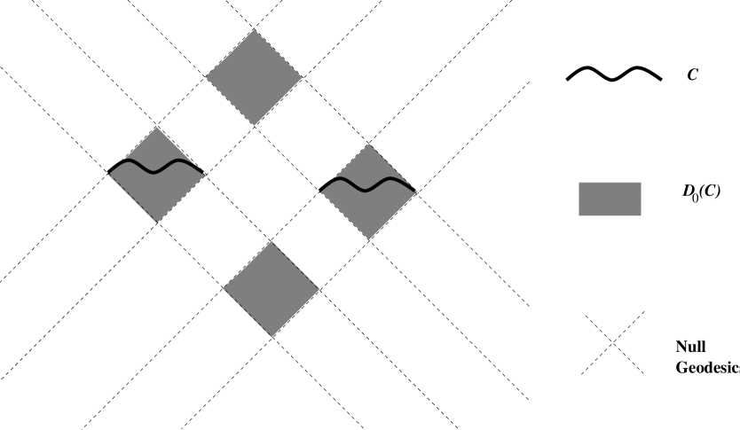
FIG. 1.: Domain of Null Dependence of $C$, $D_{0}(C)\subset L\bigcup\Sigma$

Since information travels along null geodesics we redefine the domain of dependence. Thus if $C$ is a spacelike (acausal) domain in a Lorentzian region $L\subset M$ then its domain of null dependence $D_{0}(C)$ is the set of points $p$ such that all non-terminating null curves from $p$ intersect $C$. For $C\subset L$ and $\Sigma^{\prime}\subset\Sigma$ we define $D_{0}(C\bigcup\Sigma^{\prime})$ to be all the points $p\in L$ where both null geodesics that intersect at $p$, either intersect $C$ or terminate on $\Sigma^{\prime}$, where they are not tangent.

From FIG. 1 we see that if $C$ is not connected then $D_{0}(C)$ may contain regions disjoint from $C$.

FIG. 2.: $D_{0}(C\bigcup\Sigma)\bigcup E$

Consider now a spacelike arc $C\subset L$ on which standard Cauchy data for (1) is prescribed (FIG. 2). Furthermore suppose that the domain of null dependence of $C$ intersects $\Sigma$ non-trivially, i.e. the intersection is one-dimensional. Then we show below that if a global solution exists and agrees with the data on $C$ then it is unique in $E$. Such a solution provides Cauchy data on $\Sigma$ which together with that on $C$ enables one to construct the solution on the domain of null dependence $D_{0}(C\bigcup\Sigma)$. In general no such global solution exists as will be illustrated in example 1 below.

If the intersection $D_{0}(C)\bigcap\Sigma$ is trivial then the theorem below is not applicable. In this case more than one global solution may exist compatible with the Cauchy data on $C$. Example 2 will illustrate this situation.

In section V we review the standard prescription that is adopted to construct a quantum field theory on a fixed globally hyperbolic manifold. With the aid of explicit examples, we draw attention to the obstructions that arise when one attempts to implement this prescription on a two-dimensional manifold with a degenerate metric. We offer reasons why we believe that a bounded unitary scattering matrix in the presence of non-dynamical signature change may not exist.

II Construction of coordinate systems

Given a two-dimensional manifold $(L,g^{L})$ with a (non-degenerate) Lorentzian metric $g^{L}$, a null coordinate system $(\eta_{+},\eta_{-})$ is one in which the metric may be written

$$g^{L} = \Omega^{L}(\eta_{+},\eta_{-})(d\eta_{+}\otimes d\eta_{-}+d\eta_{-}\otimes d\eta_{+})$$ (2)

where $\Omega^{L}$ is a real function. Similarly for a two-dimensional manifold $(E,g^{E})$ with a (non-degenerate) Euclidean metric $g^{E}$, a complex isothermal coordinate system $(z,\overline{z})$ is one in which the metric may written

$$g^{E} = \Omega^{E}(z,\overline{z})(dz\otimes d\overline{z}+dz\otimes d\overline{z})$$ (3)

where $\Omega^{E}$ is a real positive function. It is known that one can construct a null coordinate system about any point in $p\in L$ and that one can construct a complex isothermal coordinates system about any point $p\in E$.

In this section we give conditions for the construction of null and complex isothermal coordinate systems for a two-dimensional manifold $M=L\bigcup\Sigma\bigcup E$ with a signature changing metric $g$.

We assume that $\Sigma$ is (locally) parameterised by a $C^{\omega}$ monotonic function $\Sigma:I\mapsto\Sigma$, with $\sigma\in I\subset{\mathbb{R}}$. (The symbol $\Sigma$ will be used for both the map and its image.) Given $p\in\Sigma$, we say $\Sigma$ is null at $p$ if

$$g\left.\left(\Sigma_{\star}\frac{\partial}{\partial\sigma}\ ,\ \Sigma_{\star}\frac{\partial}{\partial\sigma}\right)\right|_{p} = 0\ .$$ (4)

If $\Sigma$ is null at $p$ then null geodesics in $L\bigcup\Sigma$ are tangent to $\Sigma$ at $p$.

For $p\in\Sigma$ such that $\Sigma$ is not null at $p$ Lemma 1 below shows that there exists a coordinate system about $p$ in $L$ which can be extended to $\Sigma$, and Lemma II.2 below shows that there exists a complex isothermal coordinate system about $p$ that extends to $\Sigma$.

Lemma II.2 is a modification of the standard proof for the existence of isothermal coordinates [18, page 455-460, vol IV]. However to simplify matters we restrict our attention to the case where $g$ is analytic and can be written in absolute time form [9] about a point $p\in\Sigma$; that is there exist coordinates $(t,x)$ about $p$ such that the metric can be written

$$g=t\,dt\otimes dt+h(t,x)^{2}dx\otimes dx$$ (5)

where $h$ is a real positive $C^{\omega}$ function. In this coordinate system the curve $\Sigma$ is given by $t=0$. Then $g^{E}$ is given by the restriction

$$g^{E}=g|_{t>0}$$ (6)

From [9, theorem 1] we know that sufficient conditions for writing $g$ in absolute time form about $p\in\Sigma$ are:

(i) $\Sigma$ is not null at $p$

(ii) with respect to any coordinate system, $\det(g_{ab})$ has a non-zero differential at $p$, and

(iii) $\{g_{ab}\}$ is $C^{\omega}$ in a neighbourhood of $p$.

With respect to both the null and complex isothermal coordinate system we then derive the general solution of (1), specifying both its value and normal derivative on $\Sigma$. This data is used to match the solutions across $\Sigma$.

Lemma 1

Extension of Null coordinate system. Given $p\in\Sigma$ such that $\Sigma$ is not null at $p$, there exists a neighbourhood of $p$, $U^{L}\subset L\bigcup\Sigma$ and a $C^{0}$ function

$$\Phi^{L}:U^{L}\mapsto{\{(\eta_{+},\eta_{-})\in{\mathbb{R}}^{2}{\ |\ }\eta_{-}\leq\eta_{+}\}}$$ (7)

such that the restriction

$$\Phi^{L}|_{L}:U^{L}\bigcap L\mapsto{\{(\eta_{+},\eta_{-})\in{\mathbb{R}}^{2}{\ |\ }\eta_{-}<\eta_{+}\}}$$ (8)

is a $C^{\infty}$ diffeomorphism and a null coordinate system. Also

$$\Phi^{L}|_{\Sigma} : U^{L}\bigcap\Sigma\mapsto{\{(\eta_{+},\eta_{-})\in{\mathbb{R}}^{2}{\ |\ }\eta_{-}=\eta_{+}\}}$$ (9)

where

$$\eta_{+}\circ\Sigma(\sigma) = \eta_{-}\circ\Sigma(\sigma)=\sigma$$ (10)

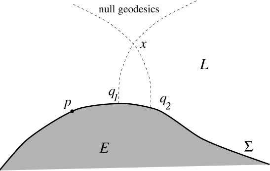
FIG. 3.: Intersection of the null geodesics from $x$ with $\Sigma$ at $q_{1}$ and $q_{2}$.

Proof II.1.

Every point $x\in L$ near $p$, lies on the intersection of two null geodesics. We can choose $U^{L}$ such that for all $x\in U^{L}\bigcap L$, both the null geodesics that intersect $x$ also intersect $\Sigma$ near $p$ where they are not tangent. Thus for each $x$ this gives two points, $q_{1},q_{2}\in\Sigma$. See FIG. 3. Let $\eta_{+}(x)$ be the larger of $\{\Sigma^{-1}(q_{1}),\Sigma^{-1}(q_{2})\}$ and $\eta_{-}(x)$ the smaller. This construction gives a well defined $C^{\infty}$ map $\Phi^{L}$, which is a diffeomorphism in the set described. Furthermore since $\eta_{\pm}={\rm constant}$ are null geodesics, $\partial/\partial\eta_{\pm}$ are null, so the metric is given by (2).

With respect to a null coordinate system the Lorentzian Hodge maps are given by

$$\star 1 = \Omega^{L}d\eta_{+}\wedge d\eta_{-}\ ,$$ (11)

$$\star d{\eta_{+}} = -d{\eta_{+}}$$ (12)

$$\star d\eta_{-} = d\eta_{-}$$ (13)

so the wave equation (1) for $\psi^{L}:U^{L}\to{\mathbb{C}}$ is

$${\displaystyle{\frac{\mbox{$\partial^{2}\psi^{L}$ }}{\mbox{$\partial{\eta_{+}}\partial\eta_{-}$}}}}d{\eta_{+}}\wedge d\eta_{-}=0\ ,$$ (14)

and its solution in this region is:

$$\psi^{L}=\psi^{L}_{+}({\eta_{+}})+\psi^{L}_{-}(\eta_{-})$$ (15)

where $\psi^{L}_{\pm}:U^{L}\to{\mathbb{C}}$. We define the value of the $\psi^{L}$ on $\Sigma$ and the normal derivative ${\cal N}\psi^{L}_{\Sigma}$ of $\psi^{L}$ on $\Sigma$ by:

$$\psi^{L}_{\Sigma} : \Sigma\mapsto{\mathbb{C}}$$ (16)

$$\psi^{L}_{\Sigma}(x) = \lim_{y\to x,\,\,y\in L}\psi^{L}(y)$$ (17)

$${\cal N}\psi^{L}_{\Sigma} : \Sigma\mapsto{\mathbb{C}}$$ (18)

$${\cal N}\psi^{L}_{\Sigma}(x) = i_{\frac{\partial}{\partial\sigma}}\left(\Sigma^{\star}\left(\lim_{y\to x,\,\,y\in L}\star d\psi^{L}|_{y}\right)\right)$$ (19)

With respect to the coordinate systems $(\eta_{+},\eta_{-})$ given in lemma 1, these are given by;

$$\psi^{L}_{\Sigma}(x) = \psi^{L}_{+}({\eta_{+}(x)})+\psi^{L}_{-}(\eta_{-}(x))$$ (20)

$${\cal N}\psi^{L}_{\Sigma}(x) = i_{\frac{\partial}{\partial\sigma}}\left(\Sigma^{\star}\lim_{y\to x,\,\,y\in L}\star d\left(\psi^{L}_{+}({\eta_{+}})+{\psi^{L}_{-}(\eta_{-})}\right)|_{y}\right)$$ (21)

$$= i_{\frac{\partial}{\partial\sigma}}\left(\Sigma^{\star}\lim_{y\to x,\,\,y\in L}\left(\psi^{L}_{+}{}^{\prime}\star d\eta_{+}+\psi^{L}_{-}{}^{\prime}\star d\eta_{-}\right)|_{y}\right)$$ (22)

$$= i_{\frac{\partial}{\partial\sigma}}\left(\Sigma^{\star}\lim_{y\to x,\,\,y\in L}\left(-\psi^{L}_{+}{}^{\prime}d\eta_{+}+\psi^{L}_{-}{}^{\prime}d\eta_{-}\right)|_{y}\right)$$ (23)

$$= i_{\frac{\partial}{\partial\sigma}}\left(\Sigma^{\star}\left(-\psi^{L}_{+}{}^{\prime}d\eta_{+}+\psi^{L}_{-}{}^{\prime}d\eta_{-}\right)|_{x}\right)$$ (24)

$$= -\psi^{L}_{+}{}^{\prime}\frac{\partial\eta_{+}\circ\Sigma}{\partial\sigma}+\psi^{L}_{-}{}^{\prime}\frac{\partial\eta_{-}\circ\Sigma}{\partial\sigma}$$ (25)

$$= -\psi^{L}_{+}{}^{\prime}(\eta_{+}(x))+\psi^{L}_{-}{}^{\prime}(\eta_{-}(x))$$ (26)

since $\partial\eta_{\pm}\circ\Sigma/\partial\sigma=1$. Thus the normal derivative exists so long as $\Sigma$ is not null.

Lemma II.2.

Extension of Complex Isothermal coordinate system. Given $p\in\Sigma$ such that $g$ is analytic and can be written in absolute time form (5) about a point $p\in\Sigma$, then there exists a neighbourhood of $p$, $U^{E}\subset E\bigcup\Sigma$ and a $C^{0}$ function

$$\Phi^{E}:U^{E}\mapsto{\{z\in{\mathbb{C}}{\ |\ }{\rm Im}(z)\geq 0\}}$$ (27)

such that the restriction

$$\Phi^{E}|_{E}:U^{E}\bigcap E\mapsto{\{z\in{\mathbb{C}}{\ |\ }{\rm Im}(z)>0\}}$$ (28)

is a $C^{\omega}$ diffeomorphism, and a complex isothermal coordinate. Also

$$\Phi^{E}|_{\Sigma} : U^{E}\bigcap\Sigma\mapsto{\mathbb{R}}$$ (29)

Proof II.3.

Let $g$ be written as in (5), so that $p$ is given by $(t=0,x=x_{0})$ and $g^{E}$ is given by (6). Let

$$\omega = h\,dx+i\sqrt{t}\,dt$$ (30)

so that

$$g^{E} = \omega\otimes\overline{\omega}+\overline{\omega}\otimes\omega\ .$$ (31)

We seek a non-vanishing integrating factor $\lambda(t,x)$, and a complex coordinate $z(t,x)$ such that

$$\omega\lambda=dz\ .$$ (32)

Consider the extension of $\omega$ to ${\mathbb{R}}^{+}\times{\mathbb{C}}$ given by

$$\omega = h(t,\xi)\,d\xi+i\sqrt{t}\,dt$$ (33)

where $t\in{\mathbb{R}},t>0$ and $\xi\in{\mathbb{C}}$, and where $h(t,\xi)$ is the analytic extension of $h(t,x)$ with respect to its second argument. Let

$$X = \frac{-i\sqrt{t}}{h}\frac{\partial}{\partial\xi}+\frac{\partial}{\partial t}\ ,$$ (34)

a vector field on ${\mathbb{R}}^{+}\times{\mathbb{C}}$, which is an annihilator of $\omega$, i.e. $\omega(X)=0$. The solution curves of $X$ are the set of curves $t\mapsto(t,\xi(t))$, where $\xi(t)$ are solutions to the differential equation:

$$\frac{dx}{dt}=-i\frac{\sqrt{t}}{h(x,t)}\ .$$ (35)

We note that the component of $X$ in the $t$ direction is 1, and the component of $X$ in the imaginary $\xi$ direction is

$$-\frac{\sqrt{t}\,{\rm Re}(h)}{|h|^{2}}$$ (36)

FIG. 4.: The solution lines of $X$ intersecting with the half plane $\{{\rm Im}(\xi)=0,t>0\}$ and the half plane $\{t=0,{\rm Im}(\xi)>0\}$ where they are parallel to the field $\partial/\partial t$.

which, near $(t=0,\xi=x_{0})$ is bounded above by $\sqrt{t}$ times some factor. Therefore near $p=(0,x_{0})$, all solution curves of (35) that intersect the half plane $\{t=0,{\rm Im}(\xi)>0\}$ also intersect the plane $\{{\rm Im}(\xi)=0,t>0\}$ and visa versa. See FIG. 4. Thus we have the map

$$\Phi^{E} : U^{E}\mapsto{\{z\in{\mathbb{C}}{\ |\ }{\rm Im}(z)\geq 0\}}$$ (37)

$$\Phi^{E} : (t,x)\mapsto z$$ (38)

where the solution curve connects the point $(t=t,{\rm Re}(\xi)=x,{\rm Im}(\xi)=0)\in\{{\rm Im}(\xi)=0,t>0\}$ to the point $(t=0,\xi=z)\in\{t=0,{\rm Im}(\xi)>0\}$. This map satisfies (28), and (29). Since $z$ now labels each solution curve, and is thus a constant along it; $X(z)\equiv dz(X)=0$. In general

$$dz = \lambda\omega+\mu_{1}\overline{\omega}+\mu_{2}dt$$ (39)

but contracting with $\partial/\partial\overline{\xi}$ implies that $\mu_{1}=0$ since $z$ and $\omega$ are analytic. Contracting with $X$ gives $\mu_{2}=0$ so (32) holds.

Substituting $dz$ into (31) gives (3) with $\Omega^{E}=1/\lambda\overline{\lambda}$.

The Euclidean Hodge maps are given with respect to the $(z,\overline{z})$ coordinate system by

$$\star 1 = \Omega^{2}dz\wedge d\overline{z}$$ (40)

$$\star d{z} = -i\;d{z}$$ (41)

$$\star d\overline{z} = i\;d\overline{z}$$ (42)

so Laplace’s equation for $\psi^{E}:U\to{\mathbb{C}}$ is

$${\displaystyle{\frac{\mbox{$\partial^{2}\psi^{E}$ }}{\mbox{$\partial{z}\partial\overline{z}$}}}}d{z}\wedge d\overline{z}=0$$ (43)

and its solution in this region is

$$\psi^{E}=\psi^{E}_{+}({z})+\overline{\psi^{E}_{-}(z)}\ ,$$ (44)

where $\psi^{E}_{\pm}:U\to{\mathbb{C}}$. Since $\partial\psi^{E}_{\pm}/\partial\overline{z}=0$ these are analytic functions. We define $\psi^{E}_{\Sigma}$ and ${\cal N}\psi^{E}_{\Sigma}$ by replacing the symbol $L$ with $E$ in (17) and (19). These are given by;

$$\psi^{E}_{\Sigma}(p) = \psi^{E}_{+}(z(p))+\overline{\psi^{E}_{-}(z(p))}$$ (45)

$${\cal N}\psi^{E}_{\Sigma}(p) = -i\psi^{E}_{+}{}^{\prime}\frac{\partial z}{\partial\sigma}+i\overline{\psi^{E}_{-}{}^{\prime}}\frac{\partial\overline{z}}{\partial\sigma}$$ (46)

We have

$$\frac{\partial z}{\partial\sigma} = \frac{dx}{d\sigma}\quad\in{\mathbb{R}}-\{0\}$$ (47)

hence

$${\cal N}\psi^{E}_{\Sigma}(p) = i\frac{dx}{d\sigma}\left(-\psi^{E}_{+}{}^{\prime}+\overline{\psi^{E}_{-}{}^{\prime}}\right)\ .$$ (48)

So the normal derivative exists about the point $p\in\Sigma$ so long as $\Sigma$ is not null.

III Uniqueness Lemma

Lemma III.4.

Let $(E\bigcup\Sigma,g)$ be a closed pathwise connected manifold with boundary $\Sigma=\partial E$, with a Riemannian metric $g$ which is degenerate on $\Sigma$ and analytic in a neighbourhood of $\Sigma$. Let there be only isolated points on $\Sigma$ about which $g$ cannot be written in absolute time form. Given a non-trivial curve $C:I\mapsto\Sigma$ where $I$ is some interval in ${\mathbb{R}}$ parameterised by $s$ and two functions $u^{E},v^{E}:E\mapsto{\mathbb{C}}$ that satisfy Laplace’s equation $d\star d\psi=0$ on the interior of $E$, then $u^{E}_{\Sigma}|_{C}=v^{E}_{\Sigma}|_{C}$ and ${\cal N}u^{E}_{\Sigma}|_{C}={\cal N}v^{E}_{\Sigma}|_{C}$ if and only if $u^{E}=v^{E}$.

In these equations $u^{E}_{\Sigma}(x),\,{\cal N}u^{E}_{\Sigma}(x)$ are defined by replacing $\psi$ by the symbol $u$ in the Euclidean version of (17),(19).

Proof III.5.

Let $(U^{E},\Psi^{E})$ be a complex isothermal chart of $E$ about a point $p\in C(I)$ given by lemma II.2 above. For the solution $w^{E}=u^{E}-v^{E}$, if follows that $w^{E}_{\Sigma}|_{C}=0$ and ${\cal N}w^{E}_{\Sigma}|_{C}=0$, thus from (45) and (48) we have

$$w^{E}_{\pm}(z) = 0\qquad\forall z\in\Psi^{E}\circ C(I)$$ (49)

hence $w^{E}_{\pm}$ are analytic functions on the domain $\Psi^{E}(U^{E}\bigcap E)\subset{\mathbb{C}}$ where ${\rm Im}(\Psi^{E}(U^{E}\bigcap E))>0$. They are continuous functions on the domain $\Psi^{E}(U^{E})\subset{\mathbb{C}}$ where ${\rm Im}(\Psi^{E}(U^{E}\bigcap\Sigma))=0$. One can perform a Schwartz reflection [19] about ${\rm Im}(z)=0$ to produce an analytic function on a domain with a non trivial subset of $\Psi^{E}(\Sigma)$ in its interior. Since $\Psi^{E}(C)$ is not a distinct collection of points

$$w^{E}_{\pm}(z) = 0\qquad\forall z\in\Psi^{E}(U^{E})\ .$$ (50)

For any other chart $(\tilde{U},\tilde{\Psi})$ where $U\bigcap\tilde{U}\neq\emptyset$, since

$$w^{E}_{\pm}(z)=0,\qquad\forall z\in\tilde{\Psi}(\tilde{U}\bigcap U)$$ (51)

then

$$w^{E}_{\pm}(z)=0,\qquad\forall z\in\tilde{\Psi}(\tilde{U})\ .$$ (52)

Thus $w^{E}_{\pm}=0$, or $u^{E}=v^{E}$ on $E$.

This is a uniqueness proof not an existence proof. Given two functions $f_{1},f_{2}:C(I)\mapsto{\mathbb{C}}$ there will in general be no solution $u:E\mapsto{\mathbb{C}}$ to Laplace’s equation such that $u|_{C}=f_{1}$ and $i_{C_{\star}\partial/\partial s}\star u=f_{2}$ for any neighbourhood of $C(I)$.

Example 1

Let $\Psi^{E}(U^{E})=\{z\in{\mathbb{C}}{\ |\ }{\rm Im}(z)<0\}$ and $\Psi^{E}(C)=\{z\in{\mathbb{C}}{\ |\ }{\rm Im}(z)=0\}$. Let

$$\psi^{E}_{\Sigma}(x) = \left\{\matrix{\displaystyle{e^{({-1/x^{2}})}}\qquad&x>0\cr 0&x\leq 0}\right.$$ (53)

$${\cal N}\psi^{E}_{\Sigma}(x) = 0\qquad\qquad\forall x\in{\mathbb{R}}$$ (54)

where $x\in\Psi^{E}(C)$. According to Lemma III.4, the data on $x<0$ implies that $\psi(z)=0\quad\forall z\in\Psi^{E}(U^{E})$, whilst the data on $x>0$ implies that $\psi(z)=\exp(-1/x^{2})\quad\forall z\in\Psi^{E}(U^{E})$. Thus there is no solution to Laplace’s equation on $\Psi^{E}(U^{E})$ consistent with this boundary data.

This does not contradict the Cauchy-Kowalewski theorem [20, 21] on the existence of solutions to PDE’s with analytic Cauchy data since the data (54) is not analytic.

IV Uniqueness Theorem

In order to match Euclidean solutions to Lorentzian solutions, we must adopt some boundary conditions along the degeneracy curve $\Sigma$.

The class of boundary conditions adopted here relate boundary data in a linear and pointwise invertible manner. Thus for $J:\Sigma\mapsto GL_{2}({\mathbb{C}})$

$$\pmatrix{\psi^{L}_{\Sigma}(x)\cr{\cal N}\psi^{L}_{\Sigma}(x)}=J(x)\pmatrix{\psi^{E}_{\Sigma}(x)\cr{\cal N}\psi^{E}_{\Sigma}(x)}$$ (55)

The “natural” boundary conditions given by continuity of $\psi$ and its normal derivative across $\Sigma$ correspond to

$$J(x)={\bf 1}.$$ (56)

We note in passing that the theorem below is applicable even when $\psi$ is restricted such that ${\cal N}\psi^{E}_{\Sigma}(x)={\cal N}\psi^{L}_{\Sigma}(x)=0$.

Theorem Let (M,g) be a two-dimensional manifold $M$ with a metric $g$ that is degenerate along a curve $\Sigma$, partitioning $M$ into a Lorentzian domain $L$ and a connected Euclidean domain $E$. Let $g$ be analytic in a neighbourhood of $\Sigma$, and let there only be isolated points on $\Sigma$ where $g$ cannot be written in absolute time form. Let $C\subset L$ be an acausal curve, parameterised by $s$, such that $D_{0}(C)\bigcap\Sigma$ contains an arc. Given two solutions of (1) $u,v:M\mapsto{\mathbb{C}}$ satisfying any boundary condition in the class above, then $u|_{C}=v|_{C}$ and $(C^{\star}\star du)(\partial/\partial s)=(C^{\star}\star dv)(\partial/\partial s)$ if and only if $u|_{D_{0}(C\bigcup\Sigma)\bigcup E}=v|_{D_{0}(C\bigcup\Sigma)\bigcup E}$ i.e. $u$ and $v$ agree on the entire shaded area indicated in FIG. 2.

Proof IV.6.

Since $u$ and $v$ have the same Cauchy data on $C$, then if $w=u-v$ it follows that $w|_{D_{0}(C)}=0$. Hence $w$ has zero Cauchy data on the Lorentzian side of $D_{0}(C)\bigcap\Sigma$ i.e.

$$w^{L}_{\Sigma}(x)=0\ \mbox{and}\ {\cal N}w^{L}_{\Sigma}(x)=0\qquad\forall x\in D_{0}(C)\bigcap\Sigma\ .$$ (57)

In these equations $w^{L}_{\Sigma}(x),\,{\cal N}w^{L}_{\Sigma}(x),\,w^{E}_{\Sigma}(x),\,{\cal N}w^{E}_{\Sigma}(x)$ are defined by replacing $\psi$ by $w$ in (17),(19). Since the boundary conditions are linear and pointwise invertible we have zero Cauchy data for $w$ on the Euclidean side of $D_{0}(C)\bigcap\Sigma$. i.e.

$$w^{E}_{\Sigma}(x)=0\ \mbox{and}\ {\cal N}w^{E}_{\Sigma}(x)=0\qquad\forall x\in D_{0}(C)\bigcap\Sigma$$ (58)

Hence $w|_{E}=0$ from Lemma III.4. This now implies zero Cauchy data for $w$ on the Euclidean side of the whole of $\Sigma$. i.e.

$$w^{E}_{\Sigma}(x)=0\ \mbox{and}\ {\cal N}w^{E}_{\Sigma}(x)=0\qquad\forall x\in\Sigma$$ (59)

Thus these boundary conditions give zero Cauchy data for $w$ on the Lorentzian side of the whole of $\Sigma$. Since the Cauchy data for $w$ on $C$ is zero as well, it follows that $w|_{D_{0}(C\bigcup\Sigma)\bigcup E}=0$.

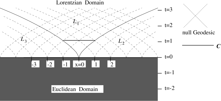
FIG. 5.: Example where $D_{0}(C)\bigcap\Sigma$ is trivial

Again we note that this is a uniqueness theorem. In general no solution to (1) on $M$ will exist satisfying (55) with Cauchy data on some $C$ satisfying the conditions of this theorem. The requirement that $D_{0}(C)\bigcap\Sigma$ is non-trivial is necessary. If the domain of null dependence of $C$ contains a single point in common with the Euclidean domain $E$ it is not difficult to construct a situation in which there exists more than one solution on $E$ compatible with the Cauchy data.

Example 2 Let $M={\mathbb{R}}^{2},\ g=-\frac{9}{4}tdt\otimes dt+dx\otimes dx$. We wish to find solutions that have zero Cauchy data on $C=\{(-1,x),-1\leq x\leq 1\}$. The null geodesics (denoted by dotted lines in FIG. 5) are given by $x\pm t^{(3/2)}=\mbox{constant}$. Clearly one solution that also satisfies the natural boundary conditions (56) is $\psi=0$ on $M$. However one readily verifies that another solution is

$$\psi|_{L}(x,t) = \left\{\vbox{ \halign{$#\hfil$&$#\hfil$&$#\hfil$&$#\hfil$&$#\hfil$&$#\hfil$&$#\hfil$\cr 0&\quad&x+t^{3/2}>0\,,&\,&x-t^{3/2}<0\,,&\,&(L_{1}\mbox{ in FIG. \ref{fig_emptyint}})\cr(1-i)\sqrt{x-t^{3/2}}&&x-t^{3/2}>0\,,&&t>0\,,&&(L_{2}\mbox{ in FIG. \ref{fig_emptyint}})\cr(1-i)\sqrt{-x-t^{3/2}}&&x+t^{3/2}>0\,,&&t>0\,,&&(L_{3}\mbox{ in FIG. \ref{fig_emptyint}})\cr}}\right.$$ (63)

$$\psi|_{E}(x,t) = \left(\sqrt{x+it^{3/2}}\right)\ +\ i\,\overline{\left(\sqrt{x+it^{3/2}}\right)}$$ (64)

where $\sqrt{\ }:\{z\in{\mathbb{C}}:{\rm Im}(z)\leq 0\}\mapsto\ \{z\in{\mathbb{C}}:{\rm Re}(z)\geq 0,\,{\rm Im}(z)\leq 0\}$.

In a two-dimensional universe with a known degenerate metric one might imagine one could use the theorem above to predict the behaviour of the scalar field beyond causally connected regions. However realistic Cauchy data that is obtained from physical measurements will contain errors. Since it is possible to find global solutions that lie arbitrarily close to such data in the domain of the Cauchy curve but are arbitrarily disparate elsewhere one must conclude that the propagation of such errors cannot be controlled. Example 3 Referring to FIG. 5, enlarge $C$ to $\widehat{C}=\{(t=1,x):|x|<2\}$. Assume the “experimental” data given on $\widehat{C}$, prescribes that a function and its normal derivative are zero to an accuracy $\epsilon$. If $\epsilon$ is zero then the theorem above implies that the only global solution is identically zero. For $\epsilon>0$, given any continuous function $f:{\mathbb{R}}\mapsto{\mathbb{C}}$ such that $f(x)=0,\ \forall|x|\leq 3$, then from the Boltzano-Wiesstrass theorem there exists a polynomial ${\cal P}:{\mathbb{R}}\mapsto{\mathbb{C}}$ such that $|{\cal P}(x)-f(x)|<\epsilon/2,\ \forall x\leq 5$. The function ${\cal P}(x+it^{3/2})$ solves Laplace’s equation (1) in the Euclidean domain and $|{\cal P}(x)|<\epsilon/2$ on the interval $\{(t=0,x):|x|<3\}$. However, this function extends to a global solution of (1) on ${\mathbb{R}}^{2}$ and is consistent with the “experimental” Cauchy data on $\widehat{C}$ within the prescribed error. This is similar to Hadamard’s example [22] demonstrating that certain initial value problems are not well posed for Laplace’s equation.

V Implications for Quantisation.

The standard method [23, 24, 25] for constructing a quantum field theory in a curved spacetime is to consider a globally hyperbolic manifold $M$ possessing Cauchy surfaces $C^{\rm in}$ and $C^{\rm out}$ in (asymptotically) flat regions upon which one sets up Hilbert spaces ${{{\cal H}(C^{\rm in})}\oplus\overline{{\cal H}(C^{\rm in})}}$ and ${{{\cal H}(C^{\rm out})}\oplus\overline{{\cal H}(C^{\rm out})}}$ of solutions to local field equations.

The Klein-Gordon hermitian bilinear form is defined as:

$$<u,v>_{C}=\frac{1}{2\pi i}\int_{C}\overline{u}\star dv-v\star d\overline{u}$$ (65)

where $u,v$ are Cauchy data on a Cauchy surface $C$ for solutions to the scalar wave (Klein-Gordon) equation. For $C$ in a flat region of spacetime the (maximal) subspace of positive frequencies, ${\cal H}(C)$, is defined by some timelike vector field which is Killing in this region, such that the restriction of $<,>_{C}$ to ${\cal H}(C)$ is positive definite. The restriction of $<,>_{C}$ to its conjugate $\overline{{\cal H}(C)}=\{\overline{u}\ |\ u\in{\cal H}(C)\}$ is negative definite. We have

$$<u,v>_{C} = <u_{+},v_{+}>_{C}+<\overline{u_{-}},\overline{v_{-}}>_{C}$$ (66)

where $u\!=\!u_{+}\!+\!\overline{u_{-}}\ ,\ v\!=\!v_{+}\!+\!\overline{v_{-}}$ and $u_{\pm},v_{\pm}\in{\cal H}(C)$. The Hilbert space ${{{\cal H}(C)}\oplus\overline{{\cal H}(C)}}$ is defined with respect to the “true” inner product

$$\ll u,v\gg_{C} = <u_{+},v_{+}>_{C}-<\overline{u_{-}},\overline{v_{-}}>_{C}\ .$$ (67)

For any solution $u\!:\!M\mapsto{\mathbb{C}}$ there is Cauchy data associated with $u^{\rm in}\in{{{\cal H}(C^{\rm in})}\oplus\overline{{\cal H}(C^{\rm in})}}$ for $u$, and Cauchy data associated with $u^{\rm out}\in{{{\cal H}(C^{\rm out})}\oplus\overline{{\cal H}(C^{\rm out})}}$. The corresponding quantum system is said to be unitary if $<u^{\rm in},v^{\rm in}>_{C^{\rm in}}=<u^{\rm out},v^{\rm out}>_{C^{\rm out}}$. This is guaranteed for a globally hyperbolic manifold since the current $\overline{u}\star du-u\star d\overline{u}$ is conserved. The linear map $\cal A:{{{\cal H}(C^{\rm in})}\oplus\overline{{\cal H}(C^{\rm in})}}\mapsto{{{\cal H}(C^{\rm out})}\oplus\overline{{\cal H}(C^{\rm out})}}$ defined by $u^{\rm in}\mapsto u^{\rm out}={\cal A}u^{\rm in}$ may be represented as

$${\cal A}=\pmatrix{\alpha&\beta\cr\overline{\beta}&\overline{\alpha}}$$ (68)

and defines the Bogolubov transformations:

$$\alpha : {{\cal H}(C^{\rm in})}\mapsto{{\cal H}(C^{\rm out})}$$ (69)

$$\beta : {{\cal H}(C^{\rm in})}\mapsto\overline{{\cal H}(C^{\rm out})}$$ (70)

From these one may construct the Scattering matrix in a Fock space basis of many particle states in the quantum theory. The expectation value of the particle number density with respect to the image of a Fock space vacuum state under this Scattering matrix can be shown to be $\sum_{ij}|\beta_{ij}|^{2}$. For a finite theory $\beta$ must be Hilbert-Schmidt. i.e. $\sum_{ij}|\beta_{ij}|^{2}<\infty$ [23, page 140]. This implies that ${\cal A}$ must be bounded.

It is of interested to see to what extent the formalism above breaks down in the context of a quantum field theory of massless scalar particles in a background two-dimensional spacetime with a degenerate metric. We approach this by considering a simple example in which we can readily calculate the Bogolubov coefficients. Let $M$ be a cylinder with coordinates $\{(\tau,\theta)|-\infty<\tau<\infty,0\leq\theta<2\pi\}$, together with the axially symmetric metric

$$g=g_{\tau\tau}(\tau)d\tau\otimes d\tau+g_{\theta\theta}(\tau)d\theta\otimes d\theta$$ (71)

where $g_{\theta\theta}(\tau)>0$ for all $\tau$. $M$ has a Euclidean region $E$ (where $g_{\tau\tau}>0$) sandwiched between two Lorentzian regions labelled $L^{\rm in}$ and $L^{\rm out}$ (where $g_{\tau\tau}<0$). Let there be a flat region $L_{\rm flat}^{\rm in}\subset L^{\rm in}$ i.e. where $g_{\tau\tau}=-1,\,g_{\theta\theta}=1$, containing the Cauchy surface $C^{\rm in}\subset L_{\rm flat}^{\rm in}$. Similarly let $C^{\rm out}\subset L_{\rm flat}^{\rm out}\subset L^{\rm out}$. Let $\Sigma^{\rm in}$ be the degeneracy ring $\tau=\tau^{\rm in}$ that partitions $E$ from $L^{\rm in}$. Similarly suppose $\Sigma^{\rm out}$ is the degeneracy ring $\tau=\tau^{\rm out}>\tau^{\rm in}$ that partitions $E$ from $L^{\rm out}$. See [15] for explicit details of such a construction.

A transformation to complex coordinates, such that the metric may be written as (3), is given by

$$z=\Psi(\tau,\theta) = e^{i\theta}\exp\left(\int_{\tau^{\rm in}}^{\tau}\left(g_{\tau\tau}(\tau^{\prime})\over g_{\theta\theta}(\tau^{\prime})\right)^{\frac{1}{2}}d\tau^{\prime}\right){\rm\ \ where\ \ }\tau^{\rm in}\leq\tau\leq\tau^{\rm out},\,\,\,0\leq\theta<2\pi$$ (72)

Thus $\Psi(E)$ is an annulus about the origin with radii $1$ and $e^{\xi}$ where

$$\xi=\int_{\tau^{\rm in}}^{\tau^{\rm out}}\left(g_{\tau\tau}(\tau^{\prime})\over g_{\theta\theta}(\tau^{\prime})\right)^{\frac{1}{2}}d\tau^{\prime}\,.$$ (73)

A convenient basis of non-zero mode solutions to (1) in the Lorentzian flat domain $L_{\rm flat}^{\rm in}$ is

$$\left\{e^{\rm in}_{k}=|2\pi k|^{-\frac{1}{2}}e^{-i(|k|\tau+k\theta)}\ ,\ \overline{e^{\rm in}_{k}}=|2\pi k|^{-\frac{1}{2}}e^{i(|k|\tau+k\theta)}\right\}_{k\in{\mathbb{Z}},\,\,k\neq 0}$$ (74)

where $(\tau,\theta)$ lie in $L_{\rm flat}^{\rm in}$. This basis is in 1-1 correspondence with the set of Cauchy data on $C^{\rm in}$ and hence provides a basis of one-particle in-states for ${{{\cal H}(C^{\rm in})}\oplus\overline{{\cal H}(C^{\rm in})}}$, with $\{e^{\rm in}_{k}\}$ giving a basis for ${\cal H}(C^{\rm in})$. A basis of one-particle out-states is likewise defined from $\{e^{\rm out}_{k},\overline{e^{\rm out}_{k}}\}$ where $(\tau,\theta)$ lie in $L_{\rm flat}^{\rm out}$.

The Bogolubov coefficients can easily be calculated from the matching conditions (56):

$$\alpha_{kk} = \cosh(k\xi)$$ (75)

$$\alpha_{kj} = 0\qquad j\neq k$$ (76)

$$\beta_{kk} = i\sinh(k\xi)$$ (77)

$$\beta_{kj} = 0\qquad j\neq k$$ (78)

It is obvious that $\beta$ is not Hilbert-Schmidt. Furthermore it is easy to verify that the linear map ${\cal A}:{{{\cal H}(C^{\rm in})}\oplus\overline{{\cal H}(C^{\rm in})}}\mapsto{{{\cal H}(C^{\rm out})}\oplus\overline{{\cal H}(C^{\rm out})}}$ is not even bounded. This follows since one can construct a solution $u$ on $M$ which has a pole on $\Sigma^{\rm out}$, e.g.

$$u(\tau,\theta)={1\over\Psi(\tau,\theta)-\Psi(\tau^{\rm out},0)}$$ (79)

Now $\|u^{\rm in}\|_{C^{\rm in}}<\infty$ but $\|u^{\rm out}\|_{C^{\rm out}}=\infty$, which could not happen if $\cal A$ were bounded. ($\|{\cal A}(u^{\rm in})\|_{C^{\rm out}}=\|u^{\rm out}\|\leq\|{\cal A}\|\,\|u^{\rm in}\|_{C^{\rm in}}$.) However on the subspace consisting of finite sums of basis elements above, the mapping $\cal A$ has a unitary restriction. Furthermore it can be shown that if $u:M\mapsto{\mathbb{C}}$ is bounded, and $u^{\rm in}\in{{{\cal H}(C^{\rm in})}\oplus\overline{{\cal H}(C^{\rm in})}}$ is it associated Cauchy data, then $<u^{\rm in},u^{\rm in}>_{C^{\rm in}}=<{\cal A}u^{\rm in},{\cal A}u^{\rm in}>_{C^{\rm out}}$ .

In order to construct ${\cal A}$ from initial Cauchy data $u^{\rm in}\in{{{\cal H}(C^{\rm in})}\oplus\overline{{\cal H}(C^{\rm in})}}$ one or more of the following obstructions may arise when attempting to calculate the corresponding element $u^{\rm out}\in{{{\cal H}(C^{\rm out})}\oplus\overline{{\cal H}(C^{\rm out})}}$:

(1) There is no compatible solution in any Euclidean neighbourhood of $\Sigma^{\rm in}$. An illustration of this has been given in example 1.

(2) Although a solution in a neighbourhood of $\Sigma^{\rm in}$ exists, this solution has a “natural boundary” which prevents it propagating to $\Sigma^{\rm out}$. For example, consider the analytic function $f:{\mathbb{D}}\mapsto{\mathbb{C}}$,

$$f(z)=\sum_{n=0}^{\infty}\left({z\over R}\right)^{(n!)}$$ (80)

where ${\mathbb{D}}\subset{\mathbb{C}}$ is the open disk of radius $R$. This function is infinite for all $z=Re^{p/q},\ p,q\in{\mathbb{Z}}$, and is therefor said to have a natural boundary on $\partial{\mathbb{D}}$. It cannot be analytically continued beyond $\partial{\mathbb{D}}$. If $1<R<e^{\xi}$ then $\Psi(\Sigma^{\rm in})\subset{\mathbb{D}}$ and $\Psi(\Sigma^{\rm out})\not\subset{\mathbb{D}}$, hence the state in ${{{\cal H}(C^{\rm in})}\oplus\overline{{\cal H}(C^{\rm in})}}$ corresponding to $f$ cannot be propagated to $\Sigma^{\rm out}$.

(3) The state propagates to $\Sigma^{\rm out}$ but contains a singularity on $\Sigma^{\rm out}$. This may give an infinite norm for the state at $C^{\rm out}$.

(4) An analytic continuation of the state on $\Sigma^{{\rm in}}$ to $\Sigma^{{\rm out}}$ exists with singularities in $E$. Such singularities can give rise to non-trivial de-Rham periods and contribute to the breakdown of unitarity. In [15] it is suggested that a resolution to this problem is to excise those domains where such solutions are singular by attaching extra tubes to the manifold. This correlates the space of allowable Cauchy data to the global topology of the manifold. One can then restore unitarity for this particular initial state by labelling some of the tubes as “in” and the others as “out”. This resolution works for any particular state but cannot be applied to the entire space of states without removing the entire Euclidean domain.

VI Conclusions

One of the most striking results of the theorem above is that a spacetime with a Euclidean domain does not necessarily require a traditional Cauchy surface in order for one to be able to predict a global solution of the (scalar) wave equation. Cauchy data on any acausal curve may be sufficient. To effect such a prediction it is only necessary: (i) that the domain of null dependence of the acausal curve has a non-trivial intersection with the Euclidean domain, (ii) the solution in the two domains is connected by “linear pointwise-invertible” junction conditions and (iii) the boundary of the Euclidean domain is a Cauchy curve for the whole Lorentzian domain. If the degenerate metric possesses a spacelike Killing isometry in the Lorentzian domain then (iii) is automatic.

For example, a two-dimensional cosmology may be modelled with a metric that is induced by appropriately immersing a paraboloid in Minkowski 3-space. If the Euclidean domain corresponds to a parabolic cap then the ring of signature change is a Cauchy curve for the prediction of solutions to the wave equation for the whole paraboloid. However every acausal segment in the Lorentzian region provides a family of (disconnected) domains of null determination. If one such domain has a non-trivial intersection with the ring of signature change then any global solution satisfying the junction conditions above can be calculated from just the Cauchy data on the original segment. However, in general, given arbitrary Cauchy data on such a segment there may be no such global solution.

Although our results have relied fundamentally on the conformal structure of the scalar wave equation and the dimensionality of the background manifold we speculate that many of these features will persist in theories that lack conformal symmetry, such as the massive Klein-Gordon Equation in three or more dimensions. The extension of our methods would exploit the general theory of Elliptic Partial Differential Equations. [20, 21, 26, 22, 27]

The traditional construction of a local quantum field theory on a spacetime relies on a number of features that are conspicuously absent on manifolds with a degenerate metric. Most notably it proves difficult to construct a space of asymptotic quantum states that can be connected by a unitary Scattering matrix.

Although it is not difficult to find subspaces of bounded Lorentzian solutions such solutions may become singular when continued to a Euclidean region via a broad class of matching conditions. Thus a well behaved Lorentzian solution can propagate into the future without attenuation and pass smoothly into a Euclidean domain where it may rapidly explode. For example for any $0<r<1$ consider the sum of two packets

$$u(\tau,\theta) = \frac{1}{1-re^{i(\theta+\widehat{\tau})}}+\frac{1}{1-re^{i(\theta-\widehat{\tau})}}$$ (81)

where

$$\widehat{\tau}=\int_{\tau}^{\tau^{\rm in}}\left(-g_{\tau\tau}(\tau^{\prime})\over g_{\theta\theta}(\tau^{\prime})\right)^{\frac{1}{2}}d\tau^{\prime}$$ (82)

for $(\tau,\theta)\in L^{\rm in}$, and

$$u(\tau,\theta) = \frac{1}{1-z}+\frac{\overline{z}}{\overline{z}-r^{2}}$$ (83)

for $(\tau,\theta)\in E$ where $z=\Psi(\tau,\theta)$ is given by (72). This is illustrated in FIG. 6, with $r=0.4$, for the cylindrical manifold $M$ above. For $\tau<\tau^{\rm in}$ the bounded Lorentzian wave packets counter-rotate around the cylinder unattenuated, until they reach the signature ring at $\tau^{\rm in}=0$. This Lorentzian solution is then matched to the Euclidean one using the junction condition (56) but with the additional constraint that the normal derivatives on either side of the degeneracy curve vanish. The solution clearly becomes an exploding peak as it diffuses into the Euclidean region, becoming singular before escaping to the Lorentzian domain.

We have also explicitly demonstrated several other obstructions than can arise when trying to construct unitary operators in a basis of asymptotic states. Although we cannot prove that no such construction is possible, the results above lead us to strongly suspect that without a radical departure from traditional methods a local unitary quantum field theory on a background with a fixed topology and degenerate metric does not exist. This conclusion does not necessarily rule out classical geometries with signature change. A more comprehensive analysis would consider a coupled field and geometry system with dynamic topology. Such a quantum geometry would then allow classical histories describing a manifold with a topology consistent with the corresponding bounded global field configuration. In the weak-field semi-classical limit such coupled states might select a self-consistent classical background geometry with a degenerate metric upon which one could construct an approximate quantum matter field description.

FIG. 6.: Evolution with $\tau$ of the modulus of a pair of counter rotating Lorentzian wavepackets $u$ across a metric degeneracy at $\tau=0$. The angular coordinate for the cylindrical manifold is denoted by $0\leq\theta<2\pi$.

VII Acknowledgements

This work has benefited from useful discussions with Charles Wang and Jörg Schray. J G is grateful to the University of Lancaster for a University Research Studentship and the Royal Society of London for a European Junior Fellowship. R W T is grateful for support from the Human Capital and Mobility Programme of the EC.

REFERENCES

- [1] R Geroch. Domain of dependence. Journal Maths Physics, 11:437, 1970.
- [2] W Kundt. Non-existence of trouser-worlds. Comm. Math. Phys., 4:143, 1967.
- [3] G W Gibbons. The elliptic interpretation of black-holes and quantum-mechanics. Nucl. Phys., B271:497–508, 1986.
- [4] G Ellis, A Sumeruk, D Coule, and C Hellaby. Change of signature in classical relativity. Class. Q. Grav., 9:1535–1554, 1992.
- [5] T Dereli, M Onder, and R W Tucker. A spinor model for quantum cosmology. Phys. Lett. B, 324:134–140, 1994.
- [6] T Dereli and R W Tucker. Signature dynamics in general-relativity. Class. Quantum Grav., 10:365–373, 1993.
- [7] T Dereli, M Onder, and R W Tucker. Signature transitions in quantum cosmology. Class. Quantum Grav., 10:1425–1434, 1993.
- [8] S A Hayward. Signature change in general-relativity. Classical And Quantum Gravity, 9(8):1851–1862, 1992.
- [9] M Kossowski and M Kriele. Signature type change and absolute-time in general-relativity. Classical Quant Grav, 10:1157–1164, 1993.
- [10] M Kossowski and M Kriele. Smooth and discontinuous signature type change in general-relativity. Classical Quant Grav, 10:2363–2371, 1993.
- [11] M Kossowski and M Kriele. Transverse, type changing, pseudo Riemannian metrics and the extendibility of geodesics. P Roy Soc Lond A Mat, A444:297, 1994.
- [12] R Kerner and J Martin. Change of signature and topology in a 5-dimensional cosmological model. Class. Q. Grav., 10:2111–2122, 1993.
- [13] T D Dray, C A Manogue, and R W Tucker. Scalar field equation in the presence of signature change. Phys. Rev. D, 48:2587–2590, 1993.
- [14] T Dray, C A Manogue, and R W Tucker. Gen. Rel. Grav., 23:967, 1991.
- [15] J Gratus and R W Tucker. Topology change and the propagation of massless fields. J. Math. Phys., 36(7):3353–3376, 1995.
- [16] L J Alty and C J Fewster. Initial value problems and signature change. Class. Q. Grav. 13:1129-1147, 1996.
- [17] B S Kay. Rev. Math. Phys, 167, 1992.
- [18] M Spivak. A Comprehensive Introduction to Differential Geometry, volume I-VI. Publish or Perish, Berkeley, 2nd edition, 1979.
- [19] S Lang. Complex Analysis. Springer, 2 edition, 1985.
- [20] S Mizohata. The Theory Of Partial Differential Equations. Cambridge, 1973.
- [21] R Courant and D Hilbert. Methods Of Mathematical Physics. Interscience Pub., 1962.
- [22] R Sakamoto. Hyperbolic Boundary Value Problems. Cambridge, 1982.
- [23] S A Fulling. Aspects Of Quantum Field Theory In Curved Space-Time. London Math. Soc. Texts 17. Cambridge, 1989.
- [24] R Wald. Quantum Field Theory In Curved Space-Time. Univ. Chicago Press, 1995.
- [25] R Wald. General Relativity. Univ. Chicago Press, 1984.
- [26] L Hormander. The Analysis Of Linear Partial Differential Operators. Springer, 1983-85.
- [27] A V Bitsadze. Equations of Mixed Type. Pergamon Press, 1964.