Canonical quantum gravity with new variables and loops: a report

Abstract

This is a brief and updated summary of a talk given at the International Conference on Gravitation and Cosmology that took place in Poona in December 1995. It is very brief and is mostly intended as a guide to current literature, or to keep people updated only in very broad terms on the latest developments in the subject.

I Introduction

The relationship of quantum mechanics and gravity has been a problematic one since the early attempts to quantize the theory of general relativity. There are a plethora of prima facie difficulties (see [1] for a summary) that one faces even before laying down any specific approach to the subject. This has discouraged many people away from the field. On the other hand, it is not healthy to just not attack a problem because some obvious difficulty is forecast to appear based on general considerations. It is much more reasonable to devote some effort to a detailed analysis, since in many cases the particular details of how the expected difficulty appears can lead to insights towards its cure.

Partly with this philosophy as a motivation, a group of people have been pursuing several aspects of the canonical quantization of gravity. The canonical approach faces some a priori problems of its own, like how to recover a spacetime picture from three dimensional notions quantum mechanically, or the related issue of the “problem of time” (see [2] for a review). Yet, it also seems as an appropriate setting for elucidating issues like what is exactly the space of states of the theory or how degrees of freedom and symmetries interlace in the theory. Some of these latter issues were also considered a stumbling block for the theory early on: how to characterize the space of states given that spatial diffeomorphism invariance was a symmetry and how to solve the nonpolynomial constraints of the theory quantum mechanically were one of the deterrents of early progress of the subject in the 60’s (see for instance [3]).

Unlike the difficulties mentioned at the beginning (problem of time, observables) some progress on the issue of diffeomorphism invariance, space of states and solutions to the constraints was achieved through the introduction of a new set of variables that allows to describe general relativity in terms of notions closer to Yang–Mills theory. These new variables were introduced by Ashtekar [4] about ten years ago and led to a large amount of new insights and perspectives on canonical quantum gravity. In the canonical approach one describes spacetime through the initial data on a spatial slice consisting of a three-dimensional metric $q^{ab}$ and the extrinsic curvature $K_{ab}$. The new variables replace these by a set of (densitized) triads $\tilde{E}^{a}_{i}$ and a canonically conjugate momentum that transforms under space and triad transformations as an $SO(3)$ connection $A_{a}^{i}$. The spacetime diffeomorphism invariance of general relativity translates itself into four constraints that the variables have to satisfy, three of them representing spatial diffeomorphism. The formalism is also invariant under triad rotations and this translates itself into three additional constraints that have exactly the form of an $SO(3)$ Gauss law. Therefore the reduced phase space of the theory is exactly that of an $SO(3)$ Yang–Mills theory with four additional constraints.

An additional element that enters into play is the fact that the connection $A_{a}^{i}$ is a complex quantity. If one constructs the connection and triad from a slice of a real four dimensional metric, the formalism assures that the evolution keeps everything real forever. One is simply using a complex coordinatization on a real phase space. However, in the quantum theory one has to ensure that the resulting metric and its time derivatives be real. This can be implemented through a set of “reality conditions”, a set of constraints that turns out to be second class. Another approach is to forget these constraints and then choose in the quantum theory an inner product that makes the observable quantities self-adjoint. This, in fact, may help to select the correct inner product for the theory, something the Dirac quantization procedure says nothing about [5].

An approach that has proved fruitful for the gauge invariant description of Yang–Mills theories is the use of holonomic variables, in which one codes the gauge invariant information of the theory in the holonomies along families of closed curves. One can actually build an entire quantum representation in which the wavefunctions are purely functionals of loops, called the “loop representation”. This approach was pioneered in Yang–Mills theories by Gambini and Trias [6, 7] and was applied in gravity by Rovelli and Smolin [8]. When applied to gravity, it immediately led to remarkable insights. On the one hand the diffeomorphism invariance of the theory gets naturally embodied into diffeomorphism invariance of closed curves and therefore the quantum states of the theory are knot invariants. Moreover the Hamiltonian constraint of general relativity, which embodies all the dynamical information of the theory, gets coded into a rather simple operator that acts at intersections of the knots [8, 9, 10, 11].

All these ideas were developed early on. Over the last two years there has been considerable progress in the consolidation of many of these ideas, taking them from being “handwaving” arguments to either rigorous theorems or rather extensive formulations for doing practical computations given certain assumptions. In particular new connections with knot and graph theory have been drawn. In this talk I will briefly summarize three directions in which the formalism is advancing: a) the implementation of a “generalized Wick transform” to deal with the issue of the reality conditions; b) the development of spin networks as a basis of states in the loop representation; c) The use of a lattice regularization for the Hamiltonian constraint that suggests unexpected dynamical connection between gravity and knot theory. This paper is only intended as a pointer to current literature, to which we refer the reader for additional details.

II Generalized Wick transform

As we mentioned in the introduction, the new variables are complex variables. Specifically, the connection $A_{a}^{i}=\Gamma_{a}^{i}+iK_{a}^{i}$ where $\Gamma_{a}^{i}$ is the spin connection built from the triad and $K_{a}^{i}$ is the extrinsic curvature with one index raised with the triad. As suggested before, one possible approach is to treat quantum mechanically $A$ and $\tilde{E}$ as complex independent variables and then choose an inner product that ensures that one has a real spacetime metric. The details of how this is achieved depend on at which level one wants to introduce an inner product. If one introduces an inner product before imposing the constraint, then one can simply require the metric and its Poisson bracket with the Hamiltonian to be real. However, a rather general consensus is that one only introduces a physical inner product in canonical quantization after imposing the constraints. Since neither the metric nor its Poisson bracket with the Hamiltonian commute with the constraints, one cannot make statements about them after imposing the constraints. What one has to do is to find conditions on the observables of the theory (quantities that commute with the constraints) that are equivalent to the reality of the four dimensional metric. Unfortunately, a practical impediment is that we do not know explicitly any quantities that commute with the constraints of general relativity that may be used for this purpose, and they are expected to be nonlocal expressions [12, 13]. This has led some people to be suspicious of the whole approach since one is “sweeping under the rug” of the impossibility of finding observables the problem of implementing the reality conditions. This feeling is reinforced by the fact that the complexity of the variables is crucial: one can build real connection-based formulations but they have high order nonpolynomial constraints [14]. It therefore seems one is concealing in these unsolved difficulties an important issue.

A lot of work on the subject has simply ignored the issue of the reality conditions. At a certain level, it makes sense. Suppose one is looking for solutions to the constraints of the theory, or of ways of characterizing the space of solutions. It is natural to start the search ignoring completely the inner product and then, from the solutions found, pick the ones of physical interest by requiring that they be normalizable with respect to the inner product. At that level one would then worry about having an inner product that respects the reality conditions. The big worry is: will the reality conditions force upon us an inner product such that most of the work done solving the constraints is rendered useless?

An important step away from the above worry was a recent construction introduced (in slightly different flavors) independently by Thiemann [15] and Ashtekar [16]. What follows is an account of their work. The idea is actually simple and attractive. Suppose one starts with general relativity formulated canonically in the traditional way, but using triads instead of the metric as fundamental variables. One then introduces a canonical transformation to a new set of variables given by the triad and a real connection $A_{a}^{i}=\Gamma_{a}^{i}+K_{a}^{i}$ (we use the same notation that for the complex connection used throughout the rest of the paper). The theory has a Gauss law and diffeomorphism constraints that look in terms of these variables exactly the same as those of the complex Ashtekar formulation. However, if one writes the Hamiltonian constraint of ordinary general relativity with a Lorentzian signature in spacetime, it turns out to be a nonpolynomial expression [14]. This is why the Ashtekar variables had to be complex, the complexity achieving the simplification of the Hamiltonian constraint to a polynomial expression. If one were interested in general relativity with a Euclidean signature, the Hamiltonian constraint in terms of the real variables we just introduced is exactly the same as that of the usual Ashtekar formulation, $H=\epsilon_{ijk}\tilde{E}^{a}_{i}\tilde{E}^{b}_{j}F_{ab}^{k}$. This actually has been known for quite some time [17].

The new insight consists in noticing that one can construct a canonical transformation that maps the constraints of the Euclidean theory to those of the Lorentzian theory. One can then simply work in the Euclidean theory (which is tantamount to working in the usual Ashtekar formulation but assuming that everything is real) and one knows that the resulting theory can be canonically mapped to real Lorentzian general relativity. In a sense, this procedure “legitimizes” many calculations that have been done ignoring the reality conditions and assuming the Ashtekar variables were real. The generator of the canonical transformation is actually very simple,

$$T={i\pi\over 2}\int d^{3}xK_{a}^{i}\tilde{E}^{a}_{i}.$$ (1)

The main drawback of the construction is that if one wishes to implement the canonical transformation quantum mechanically, the operator that materializes it is given by the exponential of $T$, which yields a highly complicated factor ordering for the resulting constraints. It is yet to be investigated what are the implications of this fact for the issue of the constraint algebra and other details of the canonical quantization, like the Hilbert space of solutions of constraints. On the positive side, the construction seems to work well not only for vacuum relativity but also for the theory coupled to matter. An interesting point to notice is that the proposed method maps solutions of the constraints of one theory to the other. It does not, however, map four dimensional Riemannian solutions to Lorentzian ones. However, it maps the integral curves of the Hamiltonian on the constraint surface from one theory to the other. This might lead to new dynamical insights in classical gravity. The main achievement however, is that previous calculations that were only heuristic, because they either ignored the reality conditions or outright treated the variables as real, can now find applicability in the Lorentzian domain, possibly in a rigorous way.

III Spin networks

The idea of a loop representation is to encode all the gauge invariant information of the theory into holonomies along loops. This is easily understood through the loop transform, which is one of the possible ways of defining the loop representation,

$$\psi(\gamma)=\int DA\,W_{\gamma}[A]\psi[A]$$ (2)

where $\psi[A]$ is a wavefunction in the connection representation, $W_{\gamma}[A]$ is the trace of the holonomy (Wilson loop) of the connection $A$ along the loop $\gamma$, and $DA$ is a measure in the infinite dimensional set of all connections.

This transform is analogous to a Fourier transform. One is expanding the functional $\psi[A]$ in a “basis” of functionals parameterized by a continuous parameter $\gamma$, $W_{\gamma}[A]$. Apart from the many mathematical subtleties involved in the fact that this is really a functional transform, one important difference stands out: the “basis” formed by $W_{\gamma}[A]$ is an overcomplete one. There are identities satisfied by Wilson loops, called Mandelstam identities. For instance, for the case of $SU(2)$, one has that for two loops $\alpha$ and $\beta$, as shown in figure 1,

$$W_{\alpha}[A]W_{\beta}[A]=W_{\alpha\circ\beta}[A]+W_{\alpha\circ\beta^{-1}}[A]$$ (3)

and also $W_{\gamma}[A]=W_{\gamma^{-1}}[A]$ and $W_{\alpha\circ\beta}[A]=W_{\beta\circ\alpha}[A]$, where $\circ$ denotes composition of curves at an origin, which for simplicity can be taken at the intersection of $\alpha$ and $\beta$. These identities are nonlinear and through combinations of them one can be led to many nontrivial-looking identities among Wilson loops. The identities are inherited by the wavefunctions $\psi(\gamma)$ in the loop representation.

The presence of these identities makes the space of functions of loops $\psi(\gamma)$ quite nontrivial. As an example, for various reasons one might be interested in wavefunctions that are one on smooth loops and zero on loops with intersections or kinks. It turns out that such functions would easily satisfy the Hamiltonian constraint. Unfortunately, they fail to satisfy the Mandelstam constraints. Also consider the following: the diffeomorphism constraint implies that wavefunction must be knot invariants. On the other hand, very few of the available knot invariants in the mathematical literature satisfy identities like Mandelstam’s. Actually this is not entirely true: the Mandelstam identities require that the wavefunctions have defined values on loops with intersections whereas most of the invariants of the mathematical literature are only defined for smooth loops. So one could conceive defining the values of these wavefunctions in such a way as to make them compatible with the Mandelstam identities. This procedure is, however, severely constrained [18].

FIG. 1.: The loops that intervene in the Mandelstam identity. In all cases the curves are the same, we added little separations at the intersection for a clearer visual appearance of the connectivity.

It therefore appears that it would be useful to encounter a subset of Wilson loops that would not be related through Mandelstam identities and would yet be sufficient to expand all gauge invariant functions. Rovelli and Smolin [19] noticed that spin networks provide a natural way to tabulate such a basis. In the original version, due to Penrose [20], spin networks are colored trivalent graphs in two dimensions. Colored means that to each strand connecting two vertices a number is assigned. What does this have to do with quantum gravity? A simple example can clarify this. Consider the loops depicted in figure 1, which intervene in the Mandelstam identity considered before. Now consider a diagrammatic notation as the one introduced in figure 2. It is clear that $W(\Gamma_{1})$ and $W(\Gamma_{2})$ are independent combinations of Wilson loops. One can therefore view $\Gamma_{1}$ and $\Gamma_{2}$ as spin networks and as generators of independent Wilson loops through the combinations defined. To make a long story short, this happens for all possible loops and networks. That is, given a graph in two dimensions with trivalent intersections, one can construct in a univocous way a basis of combinations of Wilson loops, that are not related through Mandelstam identities. It turns out that the reason for this is that group-theoretic considerations of recoupling theory are at the foundation of the spin network approach [21]. But for this review we will leave matters here. It suffices to say that one can now construct a representation in which wavefunctions are labelled by spin networks and one can do there whatever one wished to do in terms of loops, like define a Hamiltonian constraint [22], dynamics, define a time and true Hamiltonian [23]. Moreover, it has been shown rigorously using measures in infinite dimensional spaces that the spin network states constructed as discussed above are orthogonal [24]. In addition, certain operators measuring the area of a surface and volume of a portion of space are naturally diagonalized by the spin network basis [25]. This has profound physical implications, since it means that areas are quantized in quantum gravity. This may, for instance, lead to a new understanding of the thermodynamics of black holes, since there now is a natural discrete structure associated with the horizon and therefore one can count states and define notions of entropy for it [26].

FIG. 2.: A symbolical notation for the loops intervening in the Mandelstam identity. $\Gamma_{1}$ corresponds to $\alpha\circ\beta^{-1}$ in figure 1 (if the strands that go to the intersection were parallel, one could genuinely omit them, that is the basis for the notation). $\Gamma_{2}$ corresponds to the symmetrized combination (at a Wilson loop level): $W_{\Gamma_{2}}[A]\equiv W_{\alpha}[A]W_{\beta}[A]+W_{\alpha\circ\beta}[A]$

IV Lattice regularization and the dynamics of gravity as skein relations

One of the central issues in the construction of a quantum theory of gravity is the definition of a regularized quantum Hamiltonian constraint. There are several ab-initio difficulties one can imagine in implementing such an operator. On one hand, one has the problem that the Hamiltonian is not diffeomorphism invariant and yet the theory has a diffeomorphism constraint. Moreover, the Hamiltonian involves products of basic operators, and most regularization procedures are not diffeomorphism invariant. One can try however, to gain some feeling for the structure of the space of solutions of the theory without facing the entire list of difficulties associated with regularizing the Hamiltonian. There are several heuristic proposals for the regularization of the action of the Hamiltonian constraint in loop space [8, 9, 10, 11]. Most of these proposals end up with an operator that acts nontrivially at intersections of loops. There, the action of the operator can be split into two pieces: a diffeomorphism invariant action, consisting of a rerouting of the loops at the intersection and a diffeomorphism- and regularization-dependent prefactor. The topological piece of the action is not unique, it originates in the need to represent the curvature that arises in the Hamiltonian as a deformation of the loops and the action of the the triads as a rerouting and there are differing proposals on how to accomplish this. The prefactor absorbs the distributional nature of the functional derivatives that arise in the definition of the quantum triad operators. The implementation of such operators on the space of wavefunctions that are solutions to the diffeomorphism constraint is pretty hopeless, since the Hamiltonian by definition will have an action that maps out of that space of functions, since it is not diffeomorphism invariant. In practice, this is assured by the presence of the regularization dependent prefactors.

One particular proposal, which appeared in the context of a lattice regularization of the theory [27, 28], is to ignore the prefactors and concentrate on the topological part of the operator. By doing so, we ensure that the kernel of the operator we are considering is contained in the kernel of the Hamiltonian. On the other hand the regularization dependent prefactors can, on rather general grounds, be chosen to be nonzero (this of course is a delicate issue) in a first analysis. It turns out that a simple regularization based on lattices yields to a topological action as that shown in figure 3. In this action the Hamiltonian only acts at triple intersections $\eta_{i}$ and it displaces one of the strands going through the intersection along a direction determined by one of the other strands back ($\eta_{2}$) and forth ($\eta_{1})$. The action of the operator consists in summing similar contributions per each pair of tangents incoming to the intersection. The contribution is completed by rerouting the subloop determined by the two strands considered in the operation, as indicated by the numbers in the figure that keep track of the orientation.

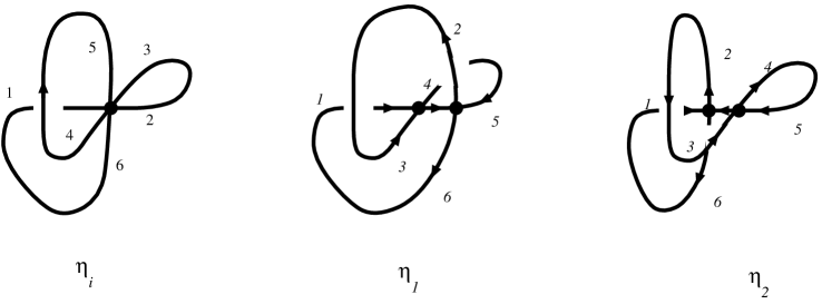
FIG. 3.: The action of the regularized Hamiltonian is only nontrivial at triple intersections $\eta_{i}$ and consists of picking a pair of strands at the intersection and moving one of them back and forth along the other. The total action is the sum of contributions along all possible pairs of strands and it also includes a rerouting of one of the two subloops defined by each pair of strands, as indicated by the numbers that keep track of orientation.

The remarkable property that this regularization has is that the second [27] and third [29] coefficient of the infinite expansion of the Jones polynomial considered in [30] are annihilated by this operator. To prove this, one considers the individual coefficient and uses its skein relations (the relations that define it as a knot invariant).

One way of viewing this result [27] is that the action of the Hamiltonian is a skein relation in itself. It is the skein relation defining the invariant that is the general solution of the quantum Einstein equations. Notice that this skein relation does not completely characterize an invariant. This is sensible, since we do not expect the quantum Einstein equations to have a single solution. It also sheds new light on how to characterize the infinite number of degrees of freedom of general relativity in terms of the topological, discrete notions of knot theory. Another upshot of this construction is that one need not worry about the algebra of constraints, since by imposing a skein relation one not only requires that the identity hold, but all possible rearrangements and multiple applications of it hold too. This makes sense in the context of diffeomorphism invariant states, where the Hamiltonian should have vanishing commutator with itself. Viewing the constraint as a skein relation therefore allows us a new perspective on the issue of the algebra of constraints. It is also worwhile remarking that in the Regge–Ponzano approach to $2+1$ gravity [31] there is an analogous situation: the constraint appears as a relation among graphs that uniquely determines the invariant that is a (in that case actually the only) solution.

It might come as a surprise to the reader that both the second and third coefficients of the infinite expansion of the Jones polynomial (which by the way are Vassiliev invariants [32]) appear as solutions. In calculations in terms of extended loops, the third coefficient was not a solution [33]. The answer to this is that this regularization is different. The calculations have some common elements with the extended loop ones but in the end lead to different results. Recall that the operator we are dealing with here is finite whereas the extended loop one required a regularization, that in turn required a counterterm to have the second coefficient be a solution [34]. We have checked that other possible candidates (for instance the square of the second coefficient) are not annihilated by the operator, which therefore has a nontrivial action. It would be interesting to see if the operator manages to annihilate all the Vassiliev invariants stemming from the Jones polynomial. The interest of these results for quantum gravity is still questionable, since only the second coefficient satisfies the Mandelstam identities and therefore can be a candidate to state of the quantum gravitational field. These results however, highlight how different regularization choices can lead to different properties of the quantum theory. It should be emphasized that both in the extended loop case and in the skein relation calculations, the fact that the knot invariants we are discussing are annihilated by the Hamiltonian constraint arises as a consequence of a very complex cancellation, involving in a very strong way properties of the knot invariants. It is remarkable that one can find two regularizations that differ in simple details and yet lead to theories with so distinct properties and of so rich a structure.

V Conclusions

In summary, progess in this area is steady. It is very encouraging to see physics emerging from these considerations, as the first steps towards calculations of the Bekenstein bound show [26]. It is also worthwhile noticing that the various sets of ideas discussed are entangling themselves in a nontrivial way, yielding a rather unexpected picture of quantum gravity. One of the most exciting aspects is that we will soon be able to tie physics deeply into the mathematics developed: for instance it is unlikely that all the regularizations of the Hamiltonian constraint proposed will lead to the correct Bekenstein bound for black holes. It is also quite likely that the mathematical developments that allow to put the theory on a more rigorous setting will act as a guideline as to what particular choices one has to make to construct the theory. The goal of a final theory of quantum gravity probably is still afar, but the fact that one is able to establish a framework that is finding its way towards concrete physical applications and yet retaining some of the original ideas that motivated it is a quite encouraging development.

- [1] C. J. Isham, gr-qc/9310031, in “Canonical gravity: from classical to quantum”, ed J. Ehlers, H. Friedrich, Lecture Notes in Physics 434, Springer-Verlag, Berlin (1994); “Structural issues in quantum gravity” gr-qc/9510063.
- [2] K. Kuchař, in “Proceedings of the 4th Canadian meeting on Relativity and Relativistic Astrophysics”, editors G. Kunstatter, D. Vincent, J. Williams, World Scientific, Singapore (1992).
- [3] B. DeWitt, Phys. Rev. 162, 195 (1967).
- [4] A. Ashtekar, Phys. Rev. Lett. 57, 2244 (1986); Phys. Rev. D36, 1587 (1987).
- [5] A. Rendall, Class. Quan. Grav. 10, 605 (1993).
- [6] R. Gambini, A. Trias, Phys. Rev. D23, 553 (1981).
- [7] R. Gambini, A. Trias, Nucl. Phys. B278, 436 (1986).
- [8] C. Rovelli, L. Smolin, Phys. Rev. Lett. 61, 1155 (1988); Nucl. Phys. B331, 80 (1990).
- [9] R. Gambini, Phys. Lett. B255, 180 (1991).
- [10] B. Brügmann, J. Pullin, Nucl. Phys. 390, 399 (1993).
- [11] M. Blencowe, Nucl. Phys. B 341, 213 (1990).
- [12] C. Torre, I. Anderson, Phys. Rev. Lett. 70, 3525 (1993); C. Torre, Phys. Rev. D48, R2373 (1993).
- [13] J. Goldberg, J. Lewandowski, C. Stornaiolo, Commun. Math. Phys. 148, 377 (1992).
- [14] F. Barbero, Phys. Rev. 49, 6935 (1994); D51, 5507 (1995);D51, 5498 (1995);
- [15] T. Thiemann, “Reality conditions inducing transforms for quantum gauge field theory and quantum gravity” preprint gr-qc/9511057.
- [16] A. Ashtekar, Phys. Rev. D53, R2865 (1996).
- [17] C. Torre, Phys. Rev. D, 3620 (1990).
- [18] R. Gambini, J. Pullin, “Variational derivations of exact skein relations for Chern–Simons theories” hep-th/9602165.
- [19] C. Rovelli, L. Smolin, Nucl. Phys. B442, 593, (1995).
- [20] R. Penrose, in “Quantum theory and beyond”, ed E. Bastin, Cambridge University Press, Cambridge (1971).
- [21] L. Kauffman, S. Lins “Temperley–Lieb recoupling theory and invariants of 3-manifolds”, Annals of Mathematics Studies 134, Princeton University Press, Princeton (1994); R. Di Pietri, C. Rovelli, gr-qc/9602023, to appear in Phys. Rev. D.
- [22] R. Borissov, “Graphical evolution of spin network states”, preprint gr-qc/9606013; R. Borissov, S. Major, L. Smolin, “The geometry of quantum spin networks”, preprint gr-qc/9512043.
- [23] C. Rovelli, J. Math. Phys.36, 6529, (1995).
- [24] J. Baez, Adv. Math. 117, 253 (1996).
- [25] C. Rovelli, L. Smolin Phys. Rev.D52, 5743, (1995).
- [26] C. Rovelli, “Black hole entropy from loop quantum gravity”, preprint gr-qc/9603063; M. Barreira, M. Carfora, C. Rovelli, “Physics from nonperturbative quantum gravity: radiation from a quantum black hole, gr-qc/9603064, to appear in Gen. Rel. Grav.
- [27] R. Gambini, J. Pullin, “The general solution of the quantum Einstein equations?” preprint gr-qc/9603019.
- [28] H. Fort, R. Gambini, J. Pullin, in preparation.
- [29] R. Gambini, J. Griego, J. Pullin, in preparation.
- [30] B. Brügmann, R. Gambini, J. Pullin, Nucl. Phys. B385, 587 (1992);Gen. Rel. Grav. 25, 1 (1993).
- [31] M. Reisenberger, and private communication.
- [32] D. Bar-Natan, Topology 34 (1995) 423-472; L. Kauffman in “Knots and quantum gravity”, J. Baez editor, Oxford, Clarendon Press (1994); J. Baez, Lett. Math. Phys. 26, 43 (1992).
- [33] J. Griego, Phys. Rev. D53 6966, (1996).
- [34] C. Di Bartolo, R. Gambini, J. Griego, Phys. Rev. D51, 502 (1995).