[

The mixmaster universe is chaotic

Abstract

For the past decade there has been a considerable debate about the existence of chaos in the mixmaster cosmological model. The debate has been hampered by the coordinate, or observer dependence of standard chaotic indicators such as Lyapunov exponents. Here we use coordinate independent, fractal methods to show the mixmaster universe is indeed chaotic.

]

The origin of the universe and the fate of collapsing stars are two of the great mysteries in nature. In general relativity without exotic matter, the singularity theorems of Hawking and Penrose [1] argue that the gravitational collapse of very massive stars ends singular and that the universe was born singular. These singular settings force gravity to face quantum mechanics. As well as exposing the fundamental laws of physics, the singular cores of black holes and the origin of the cosmos draw deep connections to the laws of thermodynamics and, as we will discuss here, to chaos.

Earlier, Khalatnikov and Lifshitz[2] argued that singular solutions were the exception rather than the rule, putting them at odds with the singularity theorems. Their argument was that deformations in spacetime would be amplified during collapse and consequently would fight the formation of a singularity. This implied that the known symmetric singular solutions were atypical. The conflict was resolved when they realized the singularity in a collapsed star could be chaotic [3]. They conjectured that a generic singularity drives spacetime to churn and oscillate chaotically. Independently, Misner [4] suggested a chaotic approach to an early universe singularity. In his mixmaster universe, the different directions in 3-space alternate in cycles of anisotropic collapse and expansion. A popular account of these developments may be found in Thorne’s recent book[5].

While the emergence of chaos helped our understanding of singularities in general relativity, building a resilient theory of relativistic chaos has become a task of its own. A debate has raged over whether or not the mixmaster universe is chaotic. Studies of the mixmaster dynamics using both approximate maps[6, 7] and numerical integrations[8, 9] have each yielded conflicting results as to the existence of positive Lyapunov exponents – a standard chaotic indicator. Finally, it was realised[9, 10] that Lyapunov exponents are coordinate dependent and the conflicting results were a consequence of the different coordinate systems. In short, Lyapunov exponents are not reliable indicators of chaos in general relativity. Using a different approach, it was shown that the mixmaster equations fail the Painlevé test[11]. This suggests that the mixmaster may be chaotic, but the Painlevé test is also inconclusive. A detailed review of the mixmaster debate can be found in Ref.[12].

In this letter we show that the mixmaster universe is indeed chaotic by using coordinate independent, fractal methods. A fractal set of self-similar universes is uncovered by numerically solving Einstein’s equations. These universes form fractal boundaries in the space of initial conditions. Such fractal partitions are the result of chaotic dynamics. We emphasize that our approach can be used to study any system described by general relativity. The mixmaster is studied here as a topical example.

The mixmaster universe[4] has closed spatial sections with the topology of a three sphere. The vacuum field equations of general relativity lead to the equations

$$(\ln a^{2})^{\prime\prime}=(b^{2}-c^{2})^{2}-a^{4}\quad{\it et\;cyc.}\;(a,b,c)\;.$$ (1)

Here $(a,b,c)$ are the scale factors for the three spatial axes, a prime denotes $d/d\tau$ and $dt=abc\,d\tau$. In a numerical study it is advantageous to use $\alpha=\ln a$, $\beta=\ln b$, $\gamma=\ln c$ and $dT=dt/(abc\ln(abc))$ as integration variables. These variables cautiously approach the curvature singularity at $t=0$. Asymptotically the new time variable is related to the comoving time $t$ by $T=\ln(\ln(1/t))$. The equations of motion (1) can be integrated to yield the Hamiltonian constraint $H=0$, where

$$H=(\ln a)^{\prime}(\ln b)^{\prime}+(\ln a)^{\prime}(\ln c)^{\prime}+(\ln b)^{\prime}(\ln c)^{\prime}$$ (2)

$$\quad-\frac{1}{4}\left[a^{4}+b^{4}+c^{4}-2\left(a^{2}b^{2}+b^{2}c^{2}+a^{2}c^{2}\right)\right]\,.$$ (3)

When the potential terms on the r.h.s. of (1) are small, the mixmaster coasts in an approximate Kasner phase described by

$$ds^{2}=-dt^{2}+t^{\,2{\textstyle p}_{{\scriptstyle a}}}dx^{2}+t^{\,2{\textstyle p}_{{\scriptstyle b}}}dy^{2}+t^{\,2{\textstyle p}_{{\scriptstyle c}}}dz^{2}\,.$$ (4)

The indices can be written as $p_{1}=(1+u)/(1+u+u^{2})$, $p_{2}=-u/(1+u+u^{2})$, and $p_{3}=(u+u^{2})/(1+u+u^{2})$, where $(a,b,c)$ can take any ordering of $(1,2,3)$ and $u\in[1,\infty)$.

Initial conditions can be set on the surface $\alpha=0$, $d\alpha/dT=\dot{\alpha}<0$, with the four variables $(u,v,s,\Sigma)$[13]:

$$\alpha=0\,,\hskip 14.45377pt\beta={\Sigma\over 1+v+uv},\hskip 7.22743pt\gamma={\Sigma(v+uv)\over 1+v+uv},$$ (5)

$$\dot{\alpha}=s\Sigma p_{1}\,,\hskip 14.45377pt\dot{\beta}=s\Sigma p_{2}\,,\hskip 14.45377pt\dot{\gamma}=s\Sigma p_{3}\,.$$ (6)

The anisotropy in the sizes and velocities of the axes is quantified by $v$ and $u$. The variables $\Sigma$ and $s$ are overall scale factors. We will primarily be interested in the evolution of $(u,v)$ as the mixmaster singularity is approached. That is, we are mostly interested in the relative rates of expansion of the three spatial directions.

Before turning to the full mixmaster dynamics, we consider the properties of a two dimensional map that approximately describes the evolution of $(u,v)$ as the singularity is approached. We use the map to guide our study of the full dynamics. A detailed comparison of our treatment and the original studies of the related Gauss map [6, 3] will be delineated elsewhere [14]. We mention that unlike previous treatments, we focus on chaotic scattering. A complete description of chaotic scattering is encoded in the unstable periodic orbits [15, 16]. These orbits form what is know as a strange repellor – a close cousin of the more familiar strange attractor. We expose the fractal nature of the repellor. The same fractal set is then found in the full dynamics.

The map evolves $(u,v)$ forward in discrete jumps[3, 13],

$$F(u,v)=\left\{\begin{array}[]{lll}u-1,&\ v+1\,,&u\geq 2\quad({\rm oscillations})\\ &&\\ {\displaystyle{1\over u-1}},&{\displaystyle{1\over v}+1}\,,&u<2\quad{\rm(bounces)}\,.\end{array}\right.$$ (7)

During an oscillation, one pair of axes oscillates out of phase while the third decreases monotonically. At a bounce, the roles of the three axes are interchanged and a different axis decreases monotonically.

The strange repellor is the fractal set of points along periodic orbits, $F^{k}(\bar{u},\bar{v})=(\bar{u},\bar{v})$. Physically these orbits are self-similar universes. Periodic orbits with period $p\leq k$ can be divided into $m$ oscillations and $k-m$ bounces. Since bounces and oscillations do not commute, the number of $u$ fixed points on an orbit with $m$ oscillations is ${}^{k}C_{m}$. The total number of fixed points at order $k$ is given by the sum over all possibilities squared, $N(k)=(2^{k}-1)^{2}$. Thus, the topological entropy[16] of the strange repellor is given by

$$H_{T}=\lim_{k\rightarrow\infty}{1\over k}\ln N(k)=2\ln 2\,.$$ (8)

Since $H_{T}>0$ the $F$-map is chaotic.

To make contact with the continuum dynamics, we display a portion of the repellor’s future invariant set in Fig. 1. The future invariant set is the collection of lines $F^{k}(\bar{u})=\bar{u}$, ($v$ arbitary). The sequence of gaps around the rationals form what is known as a Farey tree. In a complementary fashion, the repellor lies on the periodic irrationals of the irrational Farey tree [14]. A similar collection of lines occurs in each integer interval $u=[n,n+1]$, but with exponentially decreasing density. The fall off can also be understood from the combinatorics of oscillations $O$ and bounces $B$. A root in this interval corresponds to the word, $O^{(n-1)}B$. The number of $n$-letter words that can be formed from a 2-letter alphabet is $2^{n}$, so the fraction of roots in each interval is $2^{-n}$. The map and the continuum dynamics will be seen to describe the same future invariant set.

The universes which comprise the strange repellor forever repeat some prescribed cycle in $(u,v)$. In contrast, a typical mixmaster universe will launch into an infinite pattern of oscillations and bounces that never repeats. Moreover, typical universes have an invariant probability $\sim u/\ln u$ that grows with $u$[17]. As a result, typical universes scatter to $u\rightarrow\infty$ while universes on the repellor are concentrated at small $u$ values.

FIG. 1.: The map’s future invariant set in the interval $1<u<2$.

We can quantify the multifractal nature of the repellor by measuring its fractal dimensions $D_{q}$, where[16]

$$D_{q}={1\over q-1}\lim_{\epsilon\rightarrow 0}{\ln\sum_{i=1}^{N(\epsilon)}(p_{i})^{q}\over\ln\epsilon}\;.$$ (9)

Here $N(\epsilon)$ are the number of hypercubes of side length $\epsilon$ needed to cover the fractal and $p_{i}$ is the fraction of points in the $i^{{\rm th}}$ hypercube. The standard capacity dimension is recovered when $q=0$, the information dimension when $q=1$, etc. For homogeneous fractals all the various dimensions yield the same result. The dimensions $D_{q}$ are invariant under diffeomorphisms for all $q$.

Since the periodic orbits of (7) are everywhere dense, it follows that the future invariant set in Fig. 1 has $D_{0}=2$. However, points on a small period orbit are visited with greater frequency and so have a larger $p_{i}$ than high period orbits. This generates an uneven distribution which ensures that $D_{q}<2$ for $q>0$. Numerically solving for all roots up to $k=16$ we find $D_{1}=1.87\pm 0.01$, thus confirming the multifractal nature of the repellor.

If the $F$-map had been obtained from the full Einstein equations without approximation, we could conclude that the mixmaster universe is chaotic. Since approximations were made[3, 13], the possibilty remains that the full equations are integrable. The approximations may have failed to preserve some integrals of the motion, thus leading to a false chaotic signal. We show this is not the case.

Since the mixmaster phase space is not compact, any chaotic behaviour is likely to be transient. There is a standard procedure to investigate such chaotic scattering. First we identify the different asymptotic outcomes the system might have. Once outcomes are identified, several methods can be used to search for a strange repellor. The simplest method looks for a fractal pattern in plots of an appropriately defined scattering angle and impact parameter. Alternatively, the strange repellor can be hunted directly with a numerical shooting procedure called PIM triples[19].

Our prefered method is to look for fractal basin boundaries[20]. Each outcome has a basin of attraction in the space of initial conditions. We may plot these basins by assigning a different color to each outcome, and then coloring all initial conditions according to their outcome. If the boundaries between these outcomes are smooth, then the dynamics is regular. Conversely, if the boundaries are fractal, the dynamics is chaotic. The set of points belonging to the fractal boundary form the strange repellor’s future invariant set.

The power of these methods as a tool for studying chaos in general relativity is twofold. First, a fractal is a non-differentiable structure and so cannot be removed by any differentiable coordinate transformation. Thus, a fractal basin boundary provides an observer independent signal of chaos. Second, most systems in general relativity have non-compact phase spaces, so most chaos will be transient. Other coordinate independent methods of studying chaos in general relativity, such as curvature based methods[21], only work for compact systems. Previously fractal techniques were used to show there is chaos in multi-black hole spacetimes[22], and in various inflationary cosmological models[23].

As it stands, the mixmaster dynamics rarely leads to definite outcomes. For typical trajectories the sequence of oscillations and bounces continues ad infinitum as the singularity is approached. A trajectory that visits any finite value of $u$, no matter how large, will eventually return to bounce again. The way around this asymptotic backwash problem is to assign outcomes at some large, but finite distance from the scattering region. This procedure cannot lead to a false chaotic signature. At worst, it will return smooth boundaries for a chaotic system. This occurs when trajectories near the strange repellor are prematurely assigned to a particular outcome.

For the mixmaster universe, typical trajectories scatter to large $u$ values, while orbits on the repellor are concentrated at small $u$ values. Accordingly, we assign outcomes when $u$ becomes larger than some fixed number, $u_{{\rm max}}$, during a Kasner phase. Due to the system’s $SO(3)$ symetry, a large $u$ value leads to three equally likely outcomes. Physically, these are the three states of highly anisotropic expansion with $p_{1}\approx p_{2}\approx 0$ and $p_{3}\approx 1$. Thus, the space of initial conditions can be color coded depending on which axis is collapsing most quickly. We color these black for $a$, grey for $b$ and white for $c$.

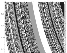
FIG. 2.: Basin boundaries in the $(u,v)$ plane for the full, unapproximated mixmaster dynamics.

Our prescription is very easy to implement numerically. In order to faciliate comparison with Fig. 1, we chose initial condition in accordance with (5) by selecting $(u_{o},v_{o})$ from a $300^{2}$ grid, setting $s_{o}=1$ and then using (2) to fix $\Sigma_{o}$. The initial conditions are then evolved according to the equations of motion (1), and the ratios of $\dot{\alpha}$, $\dot{\beta}$ and $\dot{\gamma}$ are monitored to see if the universe is in an approximate Kasner phase described by (4). If it is, the value of $u$ is extracted and an outcome is assigned if $u>u_{{\rm max}}$. We choose $u_{{\max}}=7$ since there is only a 1 in $2^{6}$ chance that a trajectory with $u>7$ lies on the strange repellor. Moreover, typical aperiodic trajectories will scatter to $u>u_{{\rm max}}$ after a few bounces, so the numerical integration is kept short and numerical errors do not become large. To confirm this, the unenforced Hamiltonian constraint (2) was monitored at all times and found to be satisfied within numerical tolerances.

In Fig. 2 we display the basin boundaries in a portion of the $(u,v)$ plane. We see a complicated mixture of both regular and fractal basin boundaries. The numerically generated basin boundaries are built of universes which ride the repellor for many orbits before being thrown off. Similar fractal basins can be found by viewing alternative slices through phase space, such as the $(\beta,\dot{\beta})$ plane. The overall morphology of the basins is altered little by demanding more strongly anisotropic outcomes. From Fig. 3 we see that the fractal nature of the boundary persists on finer and finer scales.

Aside from some mild warpage, the future invariant set (basin boundaries) seen in Figs. 2 & 3 for the full dynamics is strikingly similar to that shown in Fig. 1 for the discrete map. The warpage can be accounted for by our choice of initial conditions near the maximum of expansion, where the approximations used to derive the map break down. However, the important fine scale structure is laid down much nearer the singularity, where the map works well, and this accounts for the agreement in the detailed structure seen in Figs. 1 and 3. Indeed, a calculation[14] of the information dimension of Fig. 3 using the uncertainty exponent method yields $D_{1}=1.86\pm 0.01$, in agreement with the map.

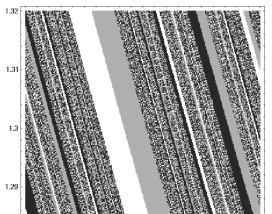
FIG. 3.: A portion of Fig. 2 magnified 25 times.

By exploiting techniques originally developed to study chaotic scattering, we gain a new perspective on the evolution of the mixmaster cosmology. We found a fractal structure, the strange repellor, describes the chaos well. The strange repellor is the collection of all universes periodic in $(u,v)$. A typical, aperiodic universe will experience a transient age of chaos if it brushes against the repellor. The fractal was exposed in both the exact Einstein equations and the discrete map used to approximate the evolution. Most importantly, our fractal approach is independent of the time coordinate used. An outcome is an outcome no matter how quickly you get there. Thus, the chaos reflected in the fractal weave of mixmaster universes is unambiguous.

It would be interesting to extend our study to include inhomogeneous collapse, and verify the connection between temporal chaos and spatial turbulence[24]. As a final comment, we note that the chaos seen in the mixmaster system occurs at large curvatures. As is well known, most of the oscillations and bounces happen after Planck scale curvatures have been reached, so quantum effects cannot be ignored. Nonetheless, our results are consistent with the contention that generic classical singularities are chaotic. This in turn suggests that quantum gravity may have to confront quantum chaos.

We thank J. Barrow, C. Dettmann, N. Frankel and P. Ferreira for helpful comments. We are grateful to C. Dettmann for letting us adapt his computer codes.

REFERENCES

- [1] S. W. Hawking & R. Penrose, Proc. R. Soc. (London), A314, 529, (1969).
- [2] E. M. Lifshitz & I. M. Khalatnikov, Sov. Phys. Uspekhi 6, 495 (1963).
- [3] I. M. Khalatnikov & E. M. Lifshitz, Phys. Rev. Lett. 24, 76 (1970); V. A. Belinskii, I. M. Khalatnikov & E. M. Lifshitz, Adv. Phys. 19, 525 (1970); ibid 31, 639 (1982).
- [4] C. W. Misner, Phys. Rev. Lett. 22, 1071, (1969).
- [5] K. Thorne, Black Holes and Time Warps: Einstein’s Outrageous Legacy, (W. W. Norton & Company, New York, 1994), Chp. 13.
- [6] J. D. Barrow, Phys. Rev. Lett. 46, 963 (1981); Phys. Rep. 85, 1 (1982).
- [7] A. B. Burd, N. Buric & R. K. Tavakol, Class. Quant. Grav. 8, 123 (1991).
- [8] G. Francisco & G. E. A. Matsas, Gen. Rel. Grav. 20, 1047 (1988).
- [9] J. Pullin, Talk given at VII Simposio Latinoamericano de Relatividad y Gravitacion, (1990).
- [10] S. E. Rugh, Cand. Scient. Thesis, The Niels Bohr Institute, (1990).
- [11] A. Latifi, M. Musette & R. Conte, Phys. Lett. A194, 83 (1994), G. Contopoulos, B. Grammaticos & A. Ramani, J. Phys. A27, 5357 (1994).
- [12] Deterministic chaos in general relativity eds. D. Hobill, A. Burd & A. Coley, (Plenum Press, New York, 1994).
- [13] D. F. Chernoff & J. D. Barrow, Phys. Rev. Lett. 50, 134 (1983).
- [14] N. J. Cornish & J. J. Levin, “The mixmaster universe: a chaotic Farey tale” (submitted to Phys. Rev. D).
- [15] P. Gaspard & S. A. Rice, J. Chem. Phys. 90, 2225 (1989); S. Bleher, C. Grebogi & E. Ott, Physica D 46, 87 (1990); O. Biham & W. Wenzel, Phys. Rev. Lett. 63, 819 (1989).
- [16] E. Ott, Chaos in dynamical systems, (Cambridge University Press, Cambridge, 1993).
- [17] B. K. Berger, Gen. Rel. Grav. 23, 1385 (1991); Phys. Rev. D47, 3222 (1993).
- [18] H. Kantz & P. Grassberger, Physica D 17, 75 (1985); T. Bohr & D. Rand, Physica D 25, 387 (1987); G. H. Hsu, E. Ott & C. Grebogi, Phys. Lett. A127, 199 (1988).
- [19] H. E. Nusse & J. Yorke, Physica D 36, 137 (1989).
- [20] C. Grebogi, E. Ott & J. A. Yorke, Phys. Rev. Lett. 50, 935 (1983).
- [21] M. Szydlowski & M. Biesiada, Phys. Rev. D 44, 2369 (1991).
- [22] C. P. Dettmann, N. E. Frankel & N. J. Cornish, Phys. Rev. D50, R618 (1994); Fractals, 3, 161 (1995).
- [23] N. J. Cornish & J. J. Levin, Phys. Rev. D53, 3022 (1996).
- [24] G. Montani, Class. Quant. Grav. 12, 2505, (1995).