COSMIC TOPOLOGY

Abstract

General relativity does not allow to specify the topology of space, leaving the possibility that space is multi– rather than simply–connected. We review the main mathematical properties of multi–connected spaces, and the different tools to classify them and to analyse their properties. Following the mathematical classification, we describe the different possible muticonnected spaces which may be used to construct universe models. We briefly discuss some implications of multi–connectedness for quantum cosmology, and its consequences concerning quantum field theory in the early universe. We consider in details the properties of the cosmological models where space is multi–connected, with emphasis towards observable effects. We then review the analyses of observational results obtained in this context, to search for a possible signature of multi–connectedness, or to constrain the models. They may concern the distribution of images of cosmic objects like galaxies, clusters, quasars,…, or more global effects, mainly those concerning the Cosmic Microwave Background, and the present limits resulting from them.

For in and out above, about, below
It is nothing but a Magic Shadow-Show
Play’d in a Box whose candle is the Sun
Round which we Phantom Figures come and go.
Omar Khayyam, $XII^{th}century$

1 Introduction

Topology plays to differential geometry a role somewhat like quantum theory to classical physics [5]. Both lead from continuous to the discrete, and at their levels relationships are more global and less local.

Topology can be applied in particular to cosmology. The purpose of relativistic cosmology is to deduce from the Einstein’s field equations some physically plausible models of the universe as a whole. However, such a program cannot be completed within the framework of general relativity only : Einstein’s equations being partial differential equations, they describe only local properties of spacetime. The latter are entirely contained in the metric tensor $g_{ij}~{}(i,j=0,1,2,3)$, or equivalently in the infinitesimal distance element $ds$ such that $ds^{2}=g_{ij}dx^{i}dx^{j}$. But Einstein’s equations do not fix the global structure – namely the topology – of the spacetime : to a given local metric element correspond several – generally an infinite number – of topologically distinct universe models.

As soon as 1917, after Einstein found [32] the first cosmological solution of general relativity – namely a static model with three–dimensional spheres ${\mathchoice{\hbox{\raise 3.41666pt\hbox to0.0pt{\kern 1.94447pt\vrule height=3.07497pt\hss}\hbox to0.0pt{\kern 3.05557pt\vrule height=3.41666pt\hss}\hbox{$\displaystyle\rm S$}}}{\hbox{\raise 3.41666pt\hbox to0.0pt{\kern 1.94447pt\vrule height=3.07497pt\hss}\hbox to0.0pt{\kern 3.05557pt\vrule height=3.41666pt\hss}\hbox{$\textstyle\rm S$}}}{\hbox{\raise 2.39166pt\hbox to0.0pt{\kern 1.36113pt\vrule height=2.15248pt\hss}\raise 0.23917pt\hbox to0.0pt{\kern 1.94444pt\vrule height=2.15248pt\hss}\hbox{$\scriptstyle\rm S$}}}{\hbox{\raise 1.70833pt\hbox to0.0pt{\kern 1.11108pt\vrule height=1.53748pt\hss}\raise 0.17084pt\hbox to0.0pt{\kern 1.52779pt\vrule height=1.53748pt\hss}\hbox{$\scriptscriptstyle\rm S$}}}}^{3}$ as spatial sections – de Sitter [25] had already noticed that the solution could also fit with a variant form of spherical space : the three-dimensional projective (or elliptical) space ${\rm I\!P}^{3}$, constructed from the 3–sphere ${\mathchoice{\hbox{\raise 3.41666pt\hbox to0.0pt{\kern 1.94447pt\vrule height=3.07497pt\hss}\hbox to0.0pt{\kern 3.05557pt\vrule height=3.41666pt\hss}\hbox{$\displaystyle\rm S$}}}{\hbox{\raise 3.41666pt\hbox to0.0pt{\kern 1.94447pt\vrule height=3.07497pt\hss}\hbox to0.0pt{\kern 3.05557pt\vrule height=3.41666pt\hss}\hbox{$\textstyle\rm S$}}}{\hbox{\raise 2.39166pt\hbox to0.0pt{\kern 1.36113pt\vrule height=2.15248pt\hss}\raise 0.23917pt\hbox to0.0pt{\kern 1.94444pt\vrule height=2.15248pt\hss}\hbox{$\scriptstyle\rm S$}}}{\hbox{\raise 1.70833pt\hbox to0.0pt{\kern 1.11108pt\vrule height=1.53748pt\hss}\raise 0.17084pt\hbox to0.0pt{\kern 1.52779pt\vrule height=1.53748pt\hss}\hbox{$\scriptscriptstyle\rm S$}}}}^{3}$ by identifying diametrically opposite points. The projective space has the same metric than the spherical space, but a different topology, with half the volume.

The discovery of non static cosmological solutions of general relativity [61, 96] enriched considerably the field of modelisation. According to the well known picture, the spatially homogeneous, isotropic Friedmann-Lemaître universe models (hereafter denoted FL) admit spatial sections of the spherical, Euclidean or hyperbolic type according when the (constant spatial) curvature is positive, zero or negative. Although it was soon recognized by Friedmann [62], Lemaître [97] and a few others [84] that the FL metrics with zero or negative curvature admitted spatially closed topologies, the idea of multi-connectedness has not attracted much support. Pioneering work in cosmic topology by Ellis [35], Sokoloff and Schvartsman [142], Zeldovich [164], Fang and Sato [57], Fagundes [46] and some others have remained widely ignored, and in almost all cosmological studies and classical textbooks, e.g. [155], it is implicitly assumed that the topology of space is simply–connected, namely that of the finite hypersphere ${\mathchoice{\hbox{\raise 3.41666pt\hbox to0.0pt{\kern 1.94447pt\vrule height=3.07497pt\hss}\hbox to0.0pt{\kern 3.05557pt\vrule height=3.41666pt\hss}\hbox{$\displaystyle\rm S$}}}{\hbox{\raise 3.41666pt\hbox to0.0pt{\kern 1.94447pt\vrule height=3.07497pt\hss}\hbox to0.0pt{\kern 3.05557pt\vrule height=3.41666pt\hss}\hbox{$\textstyle\rm S$}}}{\hbox{\raise 2.39166pt\hbox to0.0pt{\kern 1.36113pt\vrule height=2.15248pt\hss}\raise 0.23917pt\hbox to0.0pt{\kern 1.94444pt\vrule height=2.15248pt\hss}\hbox{$\scriptstyle\rm S$}}}{\hbox{\raise 1.70833pt\hbox to0.0pt{\kern 1.11108pt\vrule height=1.53748pt\hss}\raise 0.17084pt\hbox to0.0pt{\kern 1.52779pt\vrule height=1.53748pt\hss}\hbox{$\scriptscriptstyle\rm S$}}}}^{3}$, of the infinite Euclidean space ${\rm I\!R}^{3}$ or of the infinite hyperbolic space ${\rm I\!H}^{3}$, without even mentionning the multi–connected alternatives. This arbitrary simplification is at the origin of a common belief of modern cosmology according to which, in order to know if space is finite or infinite, it would be sufficient to determine the sign of its spatial curvature, or equivalently to compare its energy density to the critical “closure” value . Present astronomical data indicate that the energy density parameter in the observable Universe is less than the critical value, but this does not exclude closed space in FL solutions, with or without a cosmological constant.

Now one can ask why the universe should not have the simplest topology. Some authors use the philosophical “principle of economy” to exclude complicated topologies, but this principle is so vague that it can also be invoked to promote the contrary, for instance the topology which gives the smallest volume [83] ! Indeed, quantum cosmology provides some new insights on this question. For instance, the spontaneous birth of the universe from quantum vacuum requires the universe to have compact spacelike hypersurfaces (see e.g. [165]), and the probability is bigger for spaces of smaller volume. Since the observations suggest that the universe is locally Euclidean or hyperbolic, then its spatial topology must be non trivial. More generally, the closure of space is considered as a necessary condition in quantum theories of gravity [81].

This review will be mainly pedagogical. Since many cosmologists are unaware of how topology and cosmology can fit together and provide new highlights in universe models, we aim to present here the ”state-of-the-art” of cosmic topology in a non–technical way. The review is organized in the following manner.

In section 2, we examine whether there are any physical arguments suggesting that realistic universe models must be time-oriented and/or space-oriented.

The section 3 is devoted to the mathematical aspects of the topological classification of manifolds. Some elementary techniques are supplied to the reader and are applied in section 4 to the classification of Riemannian surfaces.

Section 5 is devoted to 3-dimensional homogeneous manifolds, and sections 6 - 7 - 8 describe the topological classification of spaces of constant curvature –those directly involved in realistic universe models.

In sections 9 - 10 we discuss the properties of multi-connected cosmological models, both at a quantum and at a classical level. The last two sections are devoted to the possible observational effects of multi-connectedness in the distribution of discrete sources (section 11) and in the distribution of continuous fields and backgrounds, in particular the Cosmic Microwave Background (section 12).

2 Spacetime orientability

The solutions of the equations of general relativity are spacetimes $({\cal M}_{4},{\bf g})$, namely 4-dimensional manifolds endowed with a Lorentzian metric  $g_{ab}$. This condition is not very restrictive, due to the following theorems (see, e.g., [66]) :

- any non-compact 4-manifold admits a Lorentzian metric

- a compact 4-manifold admits a Lorentzian metric if and only if its Euler-Poincaré characteristic  is zero.

The range of possible topological structures compatible with a given metric solution of Einstein’s equations thus remains huge, but it is clear that most of the Lorentzian 4-manifolds have no physical relevance : the building of realistic universe models sets additional restrictions. To begin, spacetime manifolds $\cal M$₄ with a boundary, or manifolds which are non–connected are likely to be eliminated. We shall assume also the manifolds to be inextendible, to ensure that all non-singular points of spacetime are included. Next come into play the conditions of time and space orientability, that we discuss in the following. More technical definitions are available elsewhere, for instance [82].

2.1 Time orientability

In the Minkowski spacetime of special relativity, particles follow worldlines from the past to the future. At any event one can define a class of future–oriented vectors and a class of past–oriented vectors. This property of local time orientability still holds in the curved spacetimes of general relativity, because special relativity remains locally valid. However, in order to define a global time orientation, that is, valid throughout the entire spacetime, the choices of local time orientations must be consistent. Namely they must vary continuously along the trajectories and, for closed trajectories, the final orientation must remain the same as the initial one.

Fortunately, to ensure the required consistency it is sufficient to test it only along certain classes of closed curves. Let us consider an arbitrary point $p\in{\cal M}_{4}$ with a closed curve $\gamma$ passing through $p$. Let fix an initial time orientation at $p$ and carry it continuously along $\gamma$. If, when returned at $p$, the orientation has not changed, the curve $\gamma$ is said to be time–preserving. By definition, a spacetime $({\cal M}_{4},\bf g)$ is time-orientable if and only if every closed curve is time-preserving.

2.2 Causality

The notion of causality, which intuitively requires that the cause precedes the effect, is a rule imposed by logics and common sense, not by the theory of relativity. Causality is implicit in special relativity, because the travel into the past is strictly equivalent to a motion along spacelike curves, which is forbidden for real particles. On the contrary, in general relativity, certain subtle distortions imprinted on curved spacetime by particular gravitational fields – for instance the one generated by a rotating black hole or a wormhole – could in principle authorize the exploration of the past while remaining inside the future light cones ([112, 73], and for a semi-popular account [99]).

However the common experience shows that, locally, different observers perceive a same preferred time–direction. In order to construct step-by-step a global time orientation, the physicist first defines a chronology. Given two events $p$ and $q$ in ${\cal M}_{4}$, $p$ is said to precede $q$ $(p\prec q)$ if there exists a continuous, timelike, future-oriented curve $\gamma$ from $p$ to $q$. The chronological future ${\cal I}^{+}(p)$ (resp. past ${\cal I}^{-}(p)$) of $p\in{\cal M}_{4}$ is the set of points $\{q\in{\cal M}_{4},p\prec q\}$ (resp. $\{q\in{\cal M}_{4},q\prec p\}$). For instance, in Minkowski spacetime, ${\cal I}^{+}(p)$ is merely the interior of the future light-cone at $p$ (figure 1).

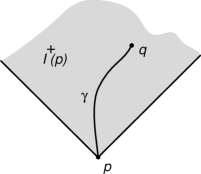
Figure 1: Chronological future in spacetime

However the chronological past and future sets may be quite pathological. This is for instance the case with the portion of Minkowski spacetime obtained by the temporal identification $(-1,x_{1},x_{2},x_{3})\equiv(+1,x_{1},x_{2},x_{3})$, where every event both belongs to its own future and past sets. More generally, if $p\in{\cal I}^{+}(p)$ for some $p\in{\cal M}_{4}$, the spacetime manifold contains closed timelike curves. This is the case for any compact spacetime, and also for some non-compact spacetimes such as the Gödel and the Taub-NUT solutions [82]. From the point of view of physics, all these manifolds are causally misbehaved and are generally ruled out as realistic universe models, although not as solutions of general relativity.

In fact, the absence of anomalies in causality is expressed fairly well by the condition of stable causality : a spacetime is stably causal if it admits a cosmic time function, that is a continuous real function $T:{\cal M}_{4}\mapsto{\rm I\!R}$, whose gradient $\nabla T$ is everywhere timelike : ${\bf g}(\nabla T(p),\nabla T(p))<0,~{}\forall p\in{\cal M}$₄.

The usual spacetimes (Minkowski, Schwarzschild, Friedmann) are stably causal. Stable causality implies global time orientability, because the time function $T$ must necessarily increase along future-oriented, null or timelike curves, and prohibits the changes of orientation along closed curves. It also allows to “slice” the spacetime into hypersurfaces of constant time function, and thus to split the spacetime metric into

$$g_{ab}=-n_{a}n_{b}+h_{ab},$$ (1)

where $n_{a}$ is the future directed normal to the hypersurface of constant time.

2.3 Global hyperbolicity

The structure of physical laws generally requires that the evolution of a system can be determined from the knowledge of its state at a given time. This is the case in classical mechanics, where the trajectory of a point mass is entirely specified by its initial position and velocity, or in quantum mechanics, where the Schrödinger equation calculates the future states knowing the present wave function.

General relativity theory also possess such a property. It is convenient to introduce the notion of domain of dependence. Given an initial spatial hypersurface $\Sigma$, its future domain of dependence ${\cal D}^{+}(\Sigma)$ (resp. past domain of dependence ${\cal D}^{-}(\Sigma)$) is the set of points $p$ such that any timelike curve reaching $p$ (resp. starting from $p$) intersects $\Sigma$. The union ${\cal D}(\Sigma)={\cal D}^{+}(\Sigma)\cup{\cal D}^{-}(\Sigma)$ is thus the region of spacetime which is entirely determined by the “information” on $\Sigma$. The problem of initial data in general relativity [21, 60] is reduced to the question of knowing the nature of the data on $\Sigma$ that specify the physics in ${\cal D}(\Sigma)$. These required initial data are determined by fixing the induced spatial metric $h_{ab}$ on $\Sigma$ and its normal derivative $K_{ab}=\frac{1}{2}L_{n}h_{ab}$, called the extrinsic curvature of $\Sigma$ in ${\cal M}$₄.

An hypersurface $\Sigma$ whose domain of dependence $D(\Sigma)$ is the whole manifold ${\cal M}$₄ is called a Cauchy surface. For instance, the hyperplane $\{t=0\}$ in Minkowski spacetime is a Cauchy surface. A spacetime which admits a Cauchy surface is said to be globally hyperbolic. A globally hyperbolic spacetime is necessarily stably causal and time–oriented (i.e., has a global time function which increases on any timelike or null curve). It is diffeomorphic to ${\rm I\!R}\times{\cal M}_{3}$, where ${\cal M}_{3}$ is a 3-dimensional riemannian manifold (with positive definite metric).

The condition of global hyperbolicity sets severe constraints on spacetime, but it is difficult to justify it on physical grounds, except if we believe in strong determinism, i.e., the wish that the entire spacetime can be calculated from the information on a single hypersurface. However we shall assume it thereafter.

2.4 Space orientability and CPT invariance

Assuming global hyperbolicity, the search for the topology of the real spacetime reduces to the exploration of the possible topologies of the spatial hypersurfaces $\cal M$₃ of constant time function [140]. May we impose additional restriction on the topology of $\cal M$₃ by assuming space orientability ? The latter can be defined in a variety of ways. It has its origine in the simple observation of surfaces : two–sided surfaces are called orientable because we can use their two–sidedness to define an orientation or a direction in ${\rm I\!R}^{3}$. This is not possible with one–sided surfaces. The simplest example, the notorious Möbius strip, is obtained by taking a rectangle and joining two ends having first twisted one of the ends. If one takes a normal ${\bf n}$ to the surface at a point $p$ and moves it continuously around the surface until it returns to $p$, it will then point in the direction ${\bf-n}$ (fig. 2). This is a sign of non–orientability. The following definition arises : any two-dimensional manifold lying in ${\rm I\!R}^{3}$ is orientable if and only if it is two-sided.

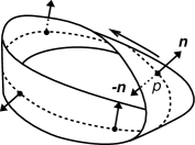
Figure 2: The non-oriented Möbius band

This can be generalized to higher dimensions. At any point of the spacetime, one can define two classes of spacelike triads : the left–handed class and the right–handed class. The spacetime is space–orientable if every closed curve preserves the spatial parity.

If time orientability can be justified on physical grounds such as the existence of an “arrow of time”, the requirement of spatial orientability is less stringent. In particle physics, the CPT theorem [149] states that any relativistic quantum field theory must be invariant under the combination of charge conjugation C, space inversion P and time reversal T. The CPT invariance is also satisfied in some versions of quantum cosmology, for instance the no–boundary proposal [80], although some authors [122] have questioned whether a full quantum gravity theory might not violate it. Until three decades ago it was commonly believed that the laws of physics were separately invariant under C, P and T transformations. Then it was experimentally discovered [159] that the weak interaction violated the parity symmetry P (or, equivalently, the CT product). Next, CP appeared to be violated in the decay of the $K_{0}$ meson [22], and other CP violations are now currently researched [156]. This series of results thus suggested that the laws of physics were not even invariant under time reversal T.

CT non invariance allows one to distinguish two possible orientations of ${\cal M}_{3}$ [160, 162], whereas CP non invariance allows one to distinguish two possible orientations of timelike vectors given on ${\cal M}_{3}$ [140]. This line of arguments leads to the strong conclusion that our spacetime must be total–orientable. Since we have assumed, from global hyperbolicity, that spacetime is already time–orientable, we conclude that the physical space must be orientable. Also, the splitting ${\cal M}_{3}\times{\rm I\!R}$ with ${\cal M}_{3}$ spacelike and orientable ensures well defined spinor fields, required by elementary particle theories to describe the variety of species of particles in the Universe [123]. We shall thus adopt this simplification in the remaining of the article.

3 Basic topology for Riemannian manifolds

3.1 What is topology ?

In simple words, topology is the mathematical framework within which to study continuity : the topological properties are those which remain insensitive to continuous transformations. Thus, size and distance are in some sense ignored in topology : stretching, squeezing or “kneading” a manifold change the metric but not the topology; cutting, tearing or making holes and handles change the latter. As a consequence, a topologist does not distinguish a triangle, a square and a circle; or a soccer ball and a rugby ball; even worse, a coffee cup and a curtain ring are the same topological entity. However, he is able to recognize the difference between a bowl and a beer mug : due to its handle, the mug cannot be continuously deformed into the bowl or into the 2–sphere ${\mathchoice{\hbox{\raise 3.41666pt\hbox to0.0pt{\kern 1.94447pt\vrule height=3.07497pt\hss}\hbox to0.0pt{\kern 3.05557pt\vrule height=3.41666pt\hss}\hbox{$\displaystyle\rm S$}}}{\hbox{\raise 3.41666pt\hbox to0.0pt{\kern 1.94447pt\vrule height=3.07497pt\hss}\hbox to0.0pt{\kern 3.05557pt\vrule height=3.41666pt\hss}\hbox{$\textstyle\rm S$}}}{\hbox{\raise 2.39166pt\hbox to0.0pt{\kern 1.36113pt\vrule height=2.15248pt\hss}\raise 0.23917pt\hbox to0.0pt{\kern 1.94444pt\vrule height=2.15248pt\hss}\hbox{$\scriptstyle\rm S$}}}{\hbox{\raise 1.70833pt\hbox to0.0pt{\kern 1.11108pt\vrule height=1.53748pt\hss}\raise 0.17084pt\hbox to0.0pt{\kern 1.52779pt\vrule height=1.53748pt\hss}\hbox{$\scriptscriptstyle\rm S$}}}}^{2}$.

Continuous transformations are mathematically depicted by homeomorphisms. If we consider two manifolds $\cal M$₁ and $\cal M$₂, a homeomorphism is a continuous map $\Phi:\cal M$${}_{1}\mapsto\cal M$₂ which has an inverse also continuous. Homeomorphisms allow one to divide the set of all possible manifolds into topologically equivalent classes : two manifolds $\cal M$₁ and $\cal M$₂ belong to the same topological class if they are homeomorphic (figure 3).

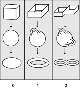
Figure 3: Classes of homeomorphic surfaces. The digits below the columns denote the number of holes, a topological invariant.

The topologist’s work is to fully characterize all equivalence classes defined from homeomorphisms and to place the manifolds in their appropriate classes. However this task is still unachieved, excepted in some restricted cases such as two–dimensional closed surfaces (section 4), three–dimensional flat (section 6) and spherical (section 7) spaces.

It is often possible to visualize two–dimensional manifolds by representing them as embedded in three–dimensional Euclidean space (such a mapping does not necessarily exist however, see below). Three–dimensional manifolds require the introduction of more abstract representations, like for instance the fundamental domain. For the sake of clarity let us illustrate our purpose by some elementary examples [137, 86].

3.2 Stories of tori

3.2.1 The two–dimensional simple torus

It has been shown since the nineteenth century that the different topological surfaces can be represented by polygons whose edges are suitably identified by pairs. Identifying one pair of opposite edges of a square gives a portion of a cylinder; then, stretching the portion of cylinder and gluing together the two circular ends generates a simple torus, a closed surface (figure 4). The torus is thus topologically equivalent to a rectangle with opposite edges identified. The rectangle is called a fundamental domain of the torus. From a topological point of view (namely without reference to size), the fundamental domain can be chosen in different ways (a rectangle, a square, …). If a turtle moves on a fundamental domain of the torus, as soon as it crosses the upper edge of the domain at a given point, it reappears on the lower opposite edge at a so-called “equivalent point” (figure 5). Many computer games where the screen plays the role of a fundamental domain are indeed played onto the surface of a torus.

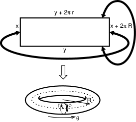
Figure 4: Construction of the flat torus

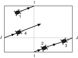
Figure 5: The turtle’s walk on a flat torus

This illustrates the difference between the metric and the topology. The torus ${\mathchoice{\hbox{\raise 3.41666pt\hbox to0.0pt{\kern 1.94447pt\vrule height=3.07497pt\hss}\hbox to0.0pt{\kern 3.05557pt\vrule height=3.41666pt\hss}\hbox{$\displaystyle\rm S$}}}{\hbox{\raise 3.41666pt\hbox to0.0pt{\kern 1.94447pt\vrule height=3.07497pt\hss}\hbox to0.0pt{\kern 3.05557pt\vrule height=3.41666pt\hss}\hbox{$\textstyle\rm S$}}}{\hbox{\raise 2.39166pt\hbox to0.0pt{\kern 1.36113pt\vrule height=2.15248pt\hss}\raise 0.23917pt\hbox to0.0pt{\kern 1.94444pt\vrule height=2.15248pt\hss}\hbox{$\scriptstyle\rm S$}}}{\hbox{\raise 1.70833pt\hbox to0.0pt{\kern 1.11108pt\vrule height=1.53748pt\hss}\raise 0.17084pt\hbox to0.0pt{\kern 1.52779pt\vrule height=1.53748pt\hss}\hbox{$\scriptscriptstyle\rm S$}}}}^{1}\times{\mathchoice{\hbox{\raise 3.41666pt\hbox to0.0pt{\kern 1.94447pt\vrule height=3.07497pt\hss}\hbox to0.0pt{\kern 3.05557pt\vrule height=3.41666pt\hss}\hbox{$\displaystyle\rm S$}}}{\hbox{\raise 3.41666pt\hbox to0.0pt{\kern 1.94447pt\vrule height=3.07497pt\hss}\hbox to0.0pt{\kern 3.05557pt\vrule height=3.41666pt\hss}\hbox{$\textstyle\rm S$}}}{\hbox{\raise 2.39166pt\hbox to0.0pt{\kern 1.36113pt\vrule height=2.15248pt\hss}\raise 0.23917pt\hbox to0.0pt{\kern 1.94444pt\vrule height=2.15248pt\hss}\hbox{$\scriptstyle\rm S$}}}{\hbox{\raise 1.70833pt\hbox to0.0pt{\kern 1.11108pt\vrule height=1.53748pt\hss}\raise 0.17084pt\hbox to0.0pt{\kern 1.52779pt\vrule height=1.53748pt\hss}\hbox{$\scriptscriptstyle\rm S$}}}}^{1}$, obtained by identification of the opposite edges of a square, is geometrically different from an usual torus $T_{1}$ (the surface of a ring for instance), which is a subset of ${\rm I\!R}^{3}$. The latter is not flat and has varying curvature, whereas ${\mathchoice{\hbox{\raise 3.41666pt\hbox to0.0pt{\kern 1.94447pt\vrule height=3.07497pt\hss}\hbox to0.0pt{\kern 3.05557pt\vrule height=3.41666pt\hss}\hbox{$\displaystyle\rm S$}}}{\hbox{\raise 3.41666pt\hbox to0.0pt{\kern 1.94447pt\vrule height=3.07497pt\hss}\hbox to0.0pt{\kern 3.05557pt\vrule height=3.41666pt\hss}\hbox{$\textstyle\rm S$}}}{\hbox{\raise 2.39166pt\hbox to0.0pt{\kern 1.36113pt\vrule height=2.15248pt\hss}\raise 0.23917pt\hbox to0.0pt{\kern 1.94444pt\vrule height=2.15248pt\hss}\hbox{$\scriptstyle\rm S$}}}{\hbox{\raise 1.70833pt\hbox to0.0pt{\kern 1.11108pt\vrule height=1.53748pt\hss}\raise 0.17084pt\hbox to0.0pt{\kern 1.52779pt\vrule height=1.53748pt\hss}\hbox{$\scriptscriptstyle\rm S$}}}}^{1}\times{\mathchoice{\hbox{\raise 3.41666pt\hbox to0.0pt{\kern 1.94447pt\vrule height=3.07497pt\hss}\hbox to0.0pt{\kern 3.05557pt\vrule height=3.41666pt\hss}\hbox{$\displaystyle\rm S$}}}{\hbox{\raise 3.41666pt\hbox to0.0pt{\kern 1.94447pt\vrule height=3.07497pt\hss}\hbox to0.0pt{\kern 3.05557pt\vrule height=3.41666pt\hss}\hbox{$\textstyle\rm S$}}}{\hbox{\raise 2.39166pt\hbox to0.0pt{\kern 1.36113pt\vrule height=2.15248pt\hss}\raise 0.23917pt\hbox to0.0pt{\kern 1.94444pt\vrule height=2.15248pt\hss}\hbox{$\scriptstyle\rm S$}}}{\hbox{\raise 1.70833pt\hbox to0.0pt{\kern 1.11108pt\vrule height=1.53748pt\hss}\raise 0.17084pt\hbox to0.0pt{\kern 1.52779pt\vrule height=1.53748pt\hss}\hbox{$\scriptscriptstyle\rm S$}}}}^{1}$ is flat everywhere and cannot be properly visualized because it cannot be immersed in ${\rm I\!R}^{3}$. It is only topologically speaking that these two tori are the same because there is an homeomorphism between them.

As food for thought we provide a more precise, although elementary, statement of this. The usual torus $T_{1}$ can be endowed with a natural riemannian metric $g_{ij}$ by taking the Euclidean metric in ${\rm I\!R}^{3}$ and imposing the restriction that the points in ${\rm I\!R}^{3}$ lie on the torus. In polar coordinates we obtain for instance

$$ds^{2}=(R+rcos\phi)^{2}(d\theta^{2}+r^{2}d\phi^{2})$$ (2)

(for the torus obtained by rotation of a circle of radius r along a circle of radius R). With respect to the metric $g_{ij}$ we have a curved torus, with a Gauss curvature

$$K=\frac{\cos\phi}{r(R+r\cos\phi)}.$$ (3)

On the other hand, the same manifold can also be given a different metric by defining a new distance between two points $t=(x,y)$ and $t^{\prime}=(x^{\prime},y^{\prime})$ as $d(t,t^{\prime})=\bigl{[}(x-x^{\prime})^{2}+(y-y^{\prime})^{2}\bigr{]}^{1/2}$. The metric becomes

$$ds^{\prime 2}=ad\theta^{2}+2bd\theta d\phi+cd\phi^{2}~{}~{}~{}(a,b,c~{}constants).$$ (4)

With respect to this metric, the torus is flat. But it cannot lie in ${\rm I\!R}^{3}$, because any two-dimensional compact connected surface in ${\rm I\!R}^{3}$ must have at least one point of non zero curvature.

3.2.2 The two–dimensional g–torus

The gluing method described above becomes extremely fruitful when the surfaces are more complicated. A two–dimensional g–torus $T_{g}$ is a torus with $g$ holes. The term “pretzel” is sometimes used in the English litterature, but the French “fougasse” (a delicious kind of bread from Provence) is still more picturesque. $T_{g}$ can be constructed as the connected sum of $g$ simple tori (figure 6). The g–torus is therefore topologically equivalent to a connected sum of $g$ squares whose opposite edges have been identified. This sum is itself topologically equivalent to a 4g–gone where all the vertices are identical with each other and the sides are suitably identified by pairs .

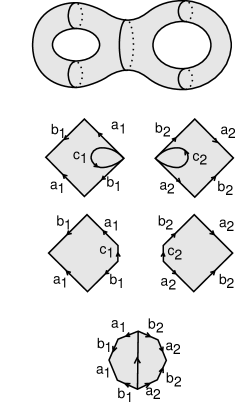
Figure 6: The two-torus as the connected sum of two simple tori.

It would be tempting to visualize the g–torus by gluing together equivalent edges, like for the simple torus. But such an operation is not straightforward when $g\geq 2$. All the vertices of the polygon correspond to the same point of the surface. Since the polygon has at least 8 edges, it is necessary to make the internal angles thinner in order to fit them suitably around a single vertex. This can only be achieved if the polygon is represented in the hyperbolic plane ${\rm I\!H}^{2}$ instead of the Euclidean plane ${\rm I\!R}^{2}$ : this increases the area and decreases the angles. The more angles to adjust, the thinner they have to be and the greater the surface. The g-torus $(g\geq 2)$ is therefore a compact surface of negative curvature.

More generally – as we shall detail in section 4 –, the sphere ${\mathchoice{\hbox{\raise 3.41666pt\hbox to0.0pt{\kern 1.94447pt\vrule height=3.07497pt\hss}\hbox to0.0pt{\kern 3.05557pt\vrule height=3.41666pt\hss}\hbox{$\displaystyle\rm S$}}}{\hbox{\raise 3.41666pt\hbox to0.0pt{\kern 1.94447pt\vrule height=3.07497pt\hss}\hbox to0.0pt{\kern 3.05557pt\vrule height=3.41666pt\hss}\hbox{$\textstyle\rm S$}}}{\hbox{\raise 2.39166pt\hbox to0.0pt{\kern 1.36113pt\vrule height=2.15248pt\hss}\raise 0.23917pt\hbox to0.0pt{\kern 1.94444pt\vrule height=2.15248pt\hss}\hbox{$\scriptstyle\rm S$}}}{\hbox{\raise 1.70833pt\hbox to0.0pt{\kern 1.11108pt\vrule height=1.53748pt\hss}\raise 0.17084pt\hbox to0.0pt{\kern 1.52779pt\vrule height=1.53748pt\hss}\hbox{$\scriptscriptstyle\rm S$}}}}^{2}~{}(g=0)$ and the g–torus $T_{g}~{}(g\geq 1)$ are the only possible compact oriented (two–sided) surfaces. $g$ is called the genus of the surface. The non–oriented surfaces are similarly defined by their genus. The major triumph of topology in the nineteenth century was the complete classification of all compact surfaces in terms of two and only two items of data : the number of holes $g$ and the orientability / non–orientability property.

It may be useful here to recall the link between the genus and the Poincaré-Euler characteristic (whose general definition was given in footnote 4). Any compact surface can be triangulated by a polyhedron. If V is the number of vertices, S the number of edges and F the number of faces, then the Poincaré-Euler characteristic reduces to $\chi=V-S+F$. It is a topological invariant, related to the genus by $g=1-\chi/2$.

3.2.3 The three–dimensional torus

When one deals with more than two dimensions, the gluing method remains the simplest way to visualize spaces. By analogy with the two-dimensional case, the three-dimensional simple torus ${\mathchoice{\hbox{\raise 3.41666pt\hbox to0.0pt{\kern 1.94447pt\vrule height=3.07497pt\hss}\hbox to0.0pt{\kern 3.05557pt\vrule height=3.41666pt\hss}\hbox{$\displaystyle\rm S$}}}{\hbox{\raise 3.41666pt\hbox to0.0pt{\kern 1.94447pt\vrule height=3.07497pt\hss}\hbox to0.0pt{\kern 3.05557pt\vrule height=3.41666pt\hss}\hbox{$\textstyle\rm S$}}}{\hbox{\raise 2.39166pt\hbox to0.0pt{\kern 1.36113pt\vrule height=2.15248pt\hss}\raise 0.23917pt\hbox to0.0pt{\kern 1.94444pt\vrule height=2.15248pt\hss}\hbox{$\scriptstyle\rm S$}}}{\hbox{\raise 1.70833pt\hbox to0.0pt{\kern 1.11108pt\vrule height=1.53748pt\hss}\raise 0.17084pt\hbox to0.0pt{\kern 1.52779pt\vrule height=1.53748pt\hss}\hbox{$\scriptscriptstyle\rm S$}}}}^{1}\times{\mathchoice{\hbox{\raise 3.41666pt\hbox to0.0pt{\kern 1.94447pt\vrule height=3.07497pt\hss}\hbox to0.0pt{\kern 3.05557pt\vrule height=3.41666pt\hss}\hbox{$\displaystyle\rm S$}}}{\hbox{\raise 3.41666pt\hbox to0.0pt{\kern 1.94447pt\vrule height=3.07497pt\hss}\hbox to0.0pt{\kern 3.05557pt\vrule height=3.41666pt\hss}\hbox{$\textstyle\rm S$}}}{\hbox{\raise 2.39166pt\hbox to0.0pt{\kern 1.36113pt\vrule height=2.15248pt\hss}\raise 0.23917pt\hbox to0.0pt{\kern 1.94444pt\vrule height=2.15248pt\hss}\hbox{$\scriptstyle\rm S$}}}{\hbox{\raise 1.70833pt\hbox to0.0pt{\kern 1.11108pt\vrule height=1.53748pt\hss}\raise 0.17084pt\hbox to0.0pt{\kern 1.52779pt\vrule height=1.53748pt\hss}\hbox{$\scriptscriptstyle\rm S$}}}}^{1}\times{\mathchoice{\hbox{\raise 3.41666pt\hbox to0.0pt{\kern 1.94447pt\vrule height=3.07497pt\hss}\hbox to0.0pt{\kern 3.05557pt\vrule height=3.41666pt\hss}\hbox{$\displaystyle\rm S$}}}{\hbox{\raise 3.41666pt\hbox to0.0pt{\kern 1.94447pt\vrule height=3.07497pt\hss}\hbox to0.0pt{\kern 3.05557pt\vrule height=3.41666pt\hss}\hbox{$\textstyle\rm S$}}}{\hbox{\raise 2.39166pt\hbox to0.0pt{\kern 1.36113pt\vrule height=2.15248pt\hss}\raise 0.23917pt\hbox to0.0pt{\kern 1.94444pt\vrule height=2.15248pt\hss}\hbox{$\scriptstyle\rm S$}}}{\hbox{\raise 1.70833pt\hbox to0.0pt{\kern 1.11108pt\vrule height=1.53748pt\hss}\raise 0.17084pt\hbox to0.0pt{\kern 1.52779pt\vrule height=1.53748pt\hss}\hbox{$\scriptscriptstyle\rm S$}}}}^{1}$ (also referred to as the hypertorus) is obtained by identifying the opposite faces of a parallelepiped such that $x=x+L_{1},~{}y=y+L_{2},~{}z=z+L_{3}$. The resulting volume is finite, equal to $L_{1}\times L_{2}\times L_{3}$. Let us imagine a light source at our position, immersed in such a structure. The light emitted backwards crosses the face of the parallelepiped behind us and reappears on the opposite face in front of us; therefore, looking forward we can see our back (as in the spherical Einstein’s universe model). Similarly, we see in our right our left profile, or upwards the bottom of our feet. In fact, as light propagates in all directions, we would observe an infinity of ghost images of any object viewed under all angles. The resulting visual effect would be comparable (although not identical) to what could be seen from inside a parallelepiped whose internal sides are covered with mirrors. Thus one would have the visual impression of infinite space, although the real space is closed. The beautiful popular article by Thurston and Weeks [152] provides a striking illustration of such a space.

More generally, any three dimensional compact manifold can be represented as a polyhedron – what we define later more precisely as the fundamental polyhedron (hereafter $FP$) – whose faces are suitably identifyied by pairs. But, as soon as the number of faces of a $FP$ exceeds 6, the compact manifold resulting from identifications cannot be developed into the Euclidean space ${\rm I\!R}^{3}$ : the $FP$ must be built in hyperbolic space ${\rm I\!H}^{3}$ in order to adjust all the angles at vertices.

3.3 Metric, Curvature and Homogeneity

3.3.1 Metric tensor

In a n-dimensional manifold $\cal{M}$, points are represented in a general coordinate system $x^{i}~{}(i=1,2,...,n)$. A coordinate line passing through a given point $P$ is obtained by varying a coordinate $x^{k}$ while keeping the other ones constant. The set $\{{\bf e}_{k}\}$ of vectors tangent to the $n$ coordinate lines at $P$ constitute a basis called the natural frame at $P$. A point $P^{\prime}$ infinitesimally close to $P$ is separated by a distance $ds=|P^{\prime}-P|$ such that $ds^{2}=g_{ij}~{}dx^{i}~{}dx^{j}$. The $g_{ij}$, which depend on coordinates $x^{k}$, are the components of the metric tensor, which is symmetric $(g_{ij}=g_{ji})$.

In the natural frame $\{{\bf e}_{k}\}$ at $P$, the infinitesimal displacement vector is ${\bf P^{\prime}}-{\bf P}={\bf e}_{k}~{}dx^{k}$ with ${\bf e_{i}.e_{j}}=g_{ij}$. The natural frame $\{{\bf e^{\prime}}_{k}\}$ at $P^{\prime}$ can be deduced from the natural frame $\{{\bf e}_{k}\}$ at $P$ by ${\bf e^{\prime}}_{i}={\bf e}_{i}+\Gamma^{j}_{ik}dx^{k}e_{j}$. The coefficients $\Gamma^{j}_{ik}$ (called Christoffel symbols) are functions of the partial derivatives of the metric tensor components, given by

$$\Gamma^{i}_{jk}={1\over 2}g^{il}\Bigl{(}{\partial g_{lj}\over\partial x^{k}}+{\partial g_{lk}\over\partial x^{j}}-{\partial g_{jk}\over\partial x^{l}}\Bigr{)}$$ (5)

where $g^{ik}g_{kj}\equiv\delta^{i}_{j}.$

3.3.2 Curvature

In any metric space, one can define the quantities

$$R^{l}_{ijk}={\partial\Gamma^{l}_{ik}\over\partial x^{j}}-{\partial\Gamma^{l}_{ij}\over\partial x^{k}}+\Gamma^{m}_{ik}\Gamma^{l}_{mj}-\Gamma^{m}_{ij}\Gamma^{l}_{mk}$$ (6)

which constitute the components of the Riemann curvature tensor. The latter contains all the information on the local geometry of the space at any given point. In Euclidean space, all the $R^{l}_{ijk}$ vanish identically at every point, which means that the construction of the natural frame in $P^{\prime}$ does not depend on the path from $P$ to $P^{\prime}$.

Describing the curvature involves “contractions” of the Riemann tensor : the Ricci tensor and the scalar curvature are respectively given by :

$$R_{ij}=R^{k}_{ikj}~{},~{}~{}~{}R=g^{ij}R_{ij}.$$ (7)

The components of the curvature tensor are not all independent. The number of independent components of $R^{l}_{ijk}$ is ${1\over 12}n^{2}(n^{2}-1)$, where $n\geq 2$ is the dimension of the manifold.

Thus for surfaces there is only one independent component, say $R_{1212}$. The Ricci tensor and the scalar curvature are respectively

$$R_{ij}=g_{ij}{R_{1212}\over det(g_{ij})}~{},~{}~{}~{}R=2{R_{1212}\over det(g_{ij})}$$ (8)

R is just (to a $-~{}\frac{1}{2}$ historical factor) the usual Gaussian curvature of the surface.

In three dimensions there are six independent components. However they do not describe the curvature in an invariant manner, that is independent of the chosen coordinate system. The invariant characterization must be formulated in terms of 3 scalars constructed from $R^{l}_{ijk}$ and $g_{ij}$. At any point P of the space one can define the Ricci principal directions or sectional curvatures, given by the roots $K_{p}$ of the characteristic equation $det(R_{ij}-\lambda g_{ij})=0$, namely :

$$K_{p}\equiv\Bigl{(}~{}R,~{}~{}R_{ij}R^{ij},~{}~{}det(R_{ij})/det(g_{ij})\Bigr{)}$$ (9)

In any dimension, a space where the relation

$$R_{ij}=\lambda~{}g_{ij},~{}~{}~{}\lambda=const$$ (10)

holds everywhere is said to have a constant curvature. In dimension 3, the sectional curvatures (9) are then all equal : they depend only on the point, not on the directions.

3.3.3 Homogeneous spaces

We have seen as an introductory example that the two–dimensional torus ${\mathchoice{\hbox{\raise 3.41666pt\hbox to0.0pt{\kern 1.94447pt\vrule height=3.07497pt\hss}\hbox to0.0pt{\kern 3.05557pt\vrule height=3.41666pt\hss}\hbox{$\displaystyle\rm S$}}}{\hbox{\raise 3.41666pt\hbox to0.0pt{\kern 1.94447pt\vrule height=3.07497pt\hss}\hbox to0.0pt{\kern 3.05557pt\vrule height=3.41666pt\hss}\hbox{$\textstyle\rm S$}}}{\hbox{\raise 2.39166pt\hbox to0.0pt{\kern 1.36113pt\vrule height=2.15248pt\hss}\raise 0.23917pt\hbox to0.0pt{\kern 1.94444pt\vrule height=2.15248pt\hss}\hbox{$\scriptstyle\rm S$}}}{\hbox{\raise 1.70833pt\hbox to0.0pt{\kern 1.11108pt\vrule height=1.53748pt\hss}\raise 0.17084pt\hbox to0.0pt{\kern 1.52779pt\vrule height=1.53748pt\hss}\hbox{$\scriptscriptstyle\rm S$}}}}^{1}\times{\mathchoice{\hbox{\raise 3.41666pt\hbox to0.0pt{\kern 1.94447pt\vrule height=3.07497pt\hss}\hbox to0.0pt{\kern 3.05557pt\vrule height=3.41666pt\hss}\hbox{$\displaystyle\rm S$}}}{\hbox{\raise 3.41666pt\hbox to0.0pt{\kern 1.94447pt\vrule height=3.07497pt\hss}\hbox to0.0pt{\kern 3.05557pt\vrule height=3.41666pt\hss}\hbox{$\textstyle\rm S$}}}{\hbox{\raise 2.39166pt\hbox to0.0pt{\kern 1.36113pt\vrule height=2.15248pt\hss}\raise 0.23917pt\hbox to0.0pt{\kern 1.94444pt\vrule height=2.15248pt\hss}\hbox{$\scriptstyle\rm S$}}}{\hbox{\raise 1.70833pt\hbox to0.0pt{\kern 1.11108pt\vrule height=1.53748pt\hss}\raise 0.17084pt\hbox to0.0pt{\kern 1.52779pt\vrule height=1.53748pt\hss}\hbox{$\scriptscriptstyle\rm S$}}}}^{1}$ has the topology of a square with opposite edges fitted together. It is thus a locally Euclidean space with constant zero curvature. Generally speaking, spaces with constant curvature (zero, positive or negative) have “nice” metrics in the sense that an observer will see the same picture wherever he stands and in whichever direction it looks. It was shown in the last century that any connected closed surface is homeomorphic to a Riemannian surface of constant curvature (ref. [77], chap.11). This major result implies that there are only three types of two–dimensional geometries, corresponding to the possible signs of their curvature : locally spherical, Euclidean, or hyperbolic.

The situation is more complicated in 3 dimensions. Obviously there are still the three constant curvature geometries ${\mathchoice{\hbox{\raise 3.41666pt\hbox to0.0pt{\kern 1.94447pt\vrule height=3.07497pt\hss}\hbox to0.0pt{\kern 3.05557pt\vrule height=3.41666pt\hss}\hbox{$\displaystyle\rm S$}}}{\hbox{\raise 3.41666pt\hbox to0.0pt{\kern 1.94447pt\vrule height=3.07497pt\hss}\hbox to0.0pt{\kern 3.05557pt\vrule height=3.41666pt\hss}\hbox{$\textstyle\rm S$}}}{\hbox{\raise 2.39166pt\hbox to0.0pt{\kern 1.36113pt\vrule height=2.15248pt\hss}\raise 0.23917pt\hbox to0.0pt{\kern 1.94444pt\vrule height=2.15248pt\hss}\hbox{$\scriptstyle\rm S$}}}{\hbox{\raise 1.70833pt\hbox to0.0pt{\kern 1.11108pt\vrule height=1.53748pt\hss}\raise 0.17084pt\hbox to0.0pt{\kern 1.52779pt\vrule height=1.53748pt\hss}\hbox{$\scriptscriptstyle\rm S$}}}}^{3}$, ${\rm I\!R}^{3}$ and ${\rm I\!H}^{3}$. But the three–dimensional cylinder ${\mathchoice{\hbox{\raise 3.41666pt\hbox to0.0pt{\kern 1.94447pt\vrule height=3.07497pt\hss}\hbox to0.0pt{\kern 3.05557pt\vrule height=3.41666pt\hss}\hbox{$\displaystyle\rm S$}}}{\hbox{\raise 3.41666pt\hbox to0.0pt{\kern 1.94447pt\vrule height=3.07497pt\hss}\hbox to0.0pt{\kern 3.05557pt\vrule height=3.41666pt\hss}\hbox{$\textstyle\rm S$}}}{\hbox{\raise 2.39166pt\hbox to0.0pt{\kern 1.36113pt\vrule height=2.15248pt\hss}\raise 0.23917pt\hbox to0.0pt{\kern 1.94444pt\vrule height=2.15248pt\hss}\hbox{$\scriptstyle\rm S$}}}{\hbox{\raise 1.70833pt\hbox to0.0pt{\kern 1.11108pt\vrule height=1.53748pt\hss}\raise 0.17084pt\hbox to0.0pt{\kern 1.52779pt\vrule height=1.53748pt\hss}\hbox{$\scriptscriptstyle\rm S$}}}}^{2}\times{\rm I\!R}$ is not homeomorphic to ${\mathchoice{\hbox{\raise 3.41666pt\hbox to0.0pt{\kern 1.94447pt\vrule height=3.07497pt\hss}\hbox to0.0pt{\kern 3.05557pt\vrule height=3.41666pt\hss}\hbox{$\displaystyle\rm S$}}}{\hbox{\raise 3.41666pt\hbox to0.0pt{\kern 1.94447pt\vrule height=3.07497pt\hss}\hbox to0.0pt{\kern 3.05557pt\vrule height=3.41666pt\hss}\hbox{$\textstyle\rm S$}}}{\hbox{\raise 2.39166pt\hbox to0.0pt{\kern 1.36113pt\vrule height=2.15248pt\hss}\raise 0.23917pt\hbox to0.0pt{\kern 1.94444pt\vrule height=2.15248pt\hss}\hbox{$\scriptstyle\rm S$}}}{\hbox{\raise 1.70833pt\hbox to0.0pt{\kern 1.11108pt\vrule height=1.53748pt\hss}\raise 0.17084pt\hbox to0.0pt{\kern 1.52779pt\vrule height=1.53748pt\hss}\hbox{$\scriptscriptstyle\rm S$}}}}^{3}$ or ${\rm I\!R}^{3}$. It can be endowed with a natural metric which is the product of the standard metrics of ${\mathchoice{\hbox{\raise 3.41666pt\hbox to0.0pt{\kern 1.94447pt\vrule height=3.07497pt\hss}\hbox to0.0pt{\kern 3.05557pt\vrule height=3.41666pt\hss}\hbox{$\displaystyle\rm S$}}}{\hbox{\raise 3.41666pt\hbox to0.0pt{\kern 1.94447pt\vrule height=3.07497pt\hss}\hbox to0.0pt{\kern 3.05557pt\vrule height=3.41666pt\hss}\hbox{$\textstyle\rm S$}}}{\hbox{\raise 2.39166pt\hbox to0.0pt{\kern 1.36113pt\vrule height=2.15248pt\hss}\raise 0.23917pt\hbox to0.0pt{\kern 1.94444pt\vrule height=2.15248pt\hss}\hbox{$\scriptstyle\rm S$}}}{\hbox{\raise 1.70833pt\hbox to0.0pt{\kern 1.11108pt\vrule height=1.53748pt\hss}\raise 0.17084pt\hbox to0.0pt{\kern 1.52779pt\vrule height=1.53748pt\hss}\hbox{$\scriptscriptstyle\rm S$}}}}^{2}$ and ${\rm I\!R}$, but this metric is anisotropic : for an observer at a given point of ${\mathchoice{\hbox{\raise 3.41666pt\hbox to0.0pt{\kern 1.94447pt\vrule height=3.07497pt\hss}\hbox to0.0pt{\kern 3.05557pt\vrule height=3.41666pt\hss}\hbox{$\displaystyle\rm S$}}}{\hbox{\raise 3.41666pt\hbox to0.0pt{\kern 1.94447pt\vrule height=3.07497pt\hss}\hbox to0.0pt{\kern 3.05557pt\vrule height=3.41666pt\hss}\hbox{$\textstyle\rm S$}}}{\hbox{\raise 2.39166pt\hbox to0.0pt{\kern 1.36113pt\vrule height=2.15248pt\hss}\raise 0.23917pt\hbox to0.0pt{\kern 1.94444pt\vrule height=2.15248pt\hss}\hbox{$\scriptstyle\rm S$}}}{\hbox{\raise 1.70833pt\hbox to0.0pt{\kern 1.11108pt\vrule height=1.53748pt\hss}\raise 0.17084pt\hbox to0.0pt{\kern 1.52779pt\vrule height=1.53748pt\hss}\hbox{$\scriptscriptstyle\rm S$}}}}^{2}\times{\rm I\!R}$, the manifold appears different in different directions; however the metric is still homogeneous in the sense that the manifold will look the same at different points. This simple example clearly shows that the three-dimensional spaces of constant curvature are just a very special case of more general homogeneous spaces. As we shall see in more details in section 5, there are eight types of homogeneous three–dimensional “geometries”, five of them not admitting a metric of constant curvature [150, 151].

Let us give mathematical substance to these notions. Quite generally, to any manifold $({\cal M},{\bf g})$ is associated a group G of isometries, i.e., transformations which leave the meric invariant. The manifold ${\cal M}$ is said homogeneous if G is non trivial  .

The group G is said to act transitively on $\cal M$ if, for any points $\bf x$ and $\bf y$ in $\cal M$ there is an isometry $g\in G$ such that $g({\bf x})={\bf y}$. The set $H$ of all points $\bf y$ in $\cal M$ such that $g({\bf x})={\bf y}$ for some $g\in G$ is called the orbit of $\bf x$. The subgroup of isometries which leave a point $\bf x$ fixed (for instance a rotation in Euclidean space) is the isotropy group $I$ at $\bf x$.

We have (theorem) :

$$dim(G)=dim(H)+dim(I).$$ (11)

If $dim(H)=dim(G)$, G is called simply transitive on $H$ (the transformation $g$ such that $g({\bf x})={\bf y}$ is unique for any $\bf x$ in $\cal M$).

If $dim(H)<dim(G)$, G is called multiply transitive.

For a n–dimensional manifold, the dimension of its full isometry group G must be $dim(G)\leq\frac{n(n+1)}{2}$ [33]. Thus, for surfaces, $dim(G)\leq 3$, and for three–dimensional Riemannian spaces, $dim(G)\leq 6$. When the dimension of the isometry group is maximum, the space is called maximally symmetric [155]. The following theorem holds : a n–dimensional manifold is maximally symmetric iff it has constant curvature.

In general relativity, manifolds are spacetimes ${\cal M}_{4}$, so that their full isometry group $G$ has necessarily $dim(G)\leq 10$.

• A spacetime with $dim(G)=10$ (that is, with constant spacetime curvature) is not physically realistic (if the curvature is zero it is the Minkowski spacetime).

• For $6<dim(G)\leq 10$, G is necessarily transitive on ${\cal M}_{4}$. Such groups have been classified by Petrov [126], but due to their high dimension they do not provide a realistic basis for cosmological models.

• For $dim(G)\leq 6$, the group may act transitively on ${\cal M}$ or else act on lower dimensional submanifolds.

  • If $G$ is simply transitive on all of ${\cal M}_{4}$, then $dim(G)=4$ and the manifold is called homogeneous in space and time. The Einstein static universe and the de Sitter universe (with positive curvature), the anti–de Sitter universe (with negative curvature) are such cases [82]. But such universe models, in which the spatial metric remains the same in time, do not admit expansion and contradict the cosmological observations.

  • If G admits a subgroup acting transitively on spacelike hypersurfaces (and not on the spacetime itself), the spacetime is said spatially homogeneous. There are still three subcases:

    • $dim(G)=6$, decomposed into a $G_{3}$ simply transitive on spacelike hypersurfaces and a $G_{3}$ isotropy group. We have the spatially homogeneous and isotropic spacetimes, admitting spacelike hypersurfaces of constant curvature (the celebrated Friedmann–Lemaître universe models). Other homogeneous spacetimes are anisotropic.

    • $dim(G)=4$ and G is multiply–transitive on 3–dimensional subspaces. Corresponding spacetimes have been considered by Kantowski and Sachs [88]. For more details, see [101] and §5.2 below.

    • $dim(G)=3$ and G is simply transitive on 3-dimensional subspaces. The corresponding groups have been classified by Bianchi [12]. See also [133, 101] and §5.2 below.

3.4 Basic tools for the topological classification of spaces

3.4.1 Connectedness, homotopy and fundamental group

The mathematical notions involved in the study and the classification of topological structures are those of multi–connectedness, homotopy, fundamental group, universal covering, holonomy, and fundamental polyhedron. All these concepts have very formal and abstract definitions that can be found in classical textbooks in topology (for instance, [106, 116] and, in the particular context of Lorentzian manifolds used in relativity, [121, 66]). In this primer we just provide pictorial definitions – with no lack of rigour, we hope – illustrated mostly in the cases of locally Euclidean surfaces.

The strategy for characterizing spaces is to produce invariants which capture the key features of the topology and uniquely specify each equivalence class. The topological invariants can take many forms. They can be just numbers, such as the dimension of the manifold, the degree of connectedness or the Poincaré – Euler characteristic. They can also be whole mathematical structures, such as the homotopy groups.

Let us introduce first the concept of homotopy. A loop at ${\bf x}\in\cal{M}$ is any path which starts at $\bf x$ and ends at $\bf x$. Two loops $\gamma$ and $\gamma^{\prime}$ are homotopic if $\gamma$ can be continuously deformed into $\gamma^{\prime}$ . The manifold $\cal{M}$ is simply–connected if, for any $\bf x$, two any loops through $\bf x$ are homotopic – or, equivalently, if every loop is homotopic to a point. If not, the manifold is said to be multi–connected. Obviously, the Euclidean spaces ${\rm I\!R}^{1}$, ${\rm I\!R}^{2}$,…, ${\rm I\!R}^{n}$, and the spheres ${\mathchoice{\hbox{\raise 3.41666pt\hbox to0.0pt{\kern 1.94447pt\vrule height=3.07497pt\hss}\hbox to0.0pt{\kern 3.05557pt\vrule height=3.41666pt\hss}\hbox{$\displaystyle\rm S$}}}{\hbox{\raise 3.41666pt\hbox to0.0pt{\kern 1.94447pt\vrule height=3.07497pt\hss}\hbox to0.0pt{\kern 3.05557pt\vrule height=3.41666pt\hss}\hbox{$\textstyle\rm S$}}}{\hbox{\raise 2.39166pt\hbox to0.0pt{\kern 1.36113pt\vrule height=2.15248pt\hss}\raise 0.23917pt\hbox to0.0pt{\kern 1.94444pt\vrule height=2.15248pt\hss}\hbox{$\scriptstyle\rm S$}}}{\hbox{\raise 1.70833pt\hbox to0.0pt{\kern 1.11108pt\vrule height=1.53748pt\hss}\raise 0.17084pt\hbox to0.0pt{\kern 1.52779pt\vrule height=1.53748pt\hss}\hbox{$\scriptscriptstyle\rm S$}}}}^{2},~{}{\mathchoice{\hbox{\raise 3.41666pt\hbox to0.0pt{\kern 1.94447pt\vrule height=3.07497pt\hss}\hbox to0.0pt{\kern 3.05557pt\vrule height=3.41666pt\hss}\hbox{$\displaystyle\rm S$}}}{\hbox{\raise 3.41666pt\hbox to0.0pt{\kern 1.94447pt\vrule height=3.07497pt\hss}\hbox to0.0pt{\kern 3.05557pt\vrule height=3.41666pt\hss}\hbox{$\textstyle\rm S$}}}{\hbox{\raise 2.39166pt\hbox to0.0pt{\kern 1.36113pt\vrule height=2.15248pt\hss}\raise 0.23917pt\hbox to0.0pt{\kern 1.94444pt\vrule height=2.15248pt\hss}\hbox{$\scriptstyle\rm S$}}}{\hbox{\raise 1.70833pt\hbox to0.0pt{\kern 1.11108pt\vrule height=1.53748pt\hss}\raise 0.17084pt\hbox to0.0pt{\kern 1.52779pt\vrule height=1.53748pt\hss}\hbox{$\scriptscriptstyle\rm S$}}}}^{3},\ldots,{\mathchoice{\hbox{\raise 3.41666pt\hbox to0.0pt{\kern 1.94447pt\vrule height=3.07497pt\hss}\hbox to0.0pt{\kern 3.05557pt\vrule height=3.41666pt\hss}\hbox{$\displaystyle\rm S$}}}{\hbox{\raise 3.41666pt\hbox to0.0pt{\kern 1.94447pt\vrule height=3.07497pt\hss}\hbox to0.0pt{\kern 3.05557pt\vrule height=3.41666pt\hss}\hbox{$\textstyle\rm S$}}}{\hbox{\raise 2.39166pt\hbox to0.0pt{\kern 1.36113pt\vrule height=2.15248pt\hss}\raise 0.23917pt\hbox to0.0pt{\kern 1.94444pt\vrule height=2.15248pt\hss}\hbox{$\scriptstyle\rm S$}}}{\hbox{\raise 1.70833pt\hbox to0.0pt{\kern 1.11108pt\vrule height=1.53748pt\hss}\raise 0.17084pt\hbox to0.0pt{\kern 1.52779pt\vrule height=1.53748pt\hss}\hbox{$\scriptscriptstyle\rm S$}}}}^{n}$ are simply–connected, whereas the circle ${\mathchoice{\hbox{\raise 3.41666pt\hbox to0.0pt{\kern 1.94447pt\vrule height=3.07497pt\hss}\hbox to0.0pt{\kern 3.05557pt\vrule height=3.41666pt\hss}\hbox{$\displaystyle\rm S$}}}{\hbox{\raise 3.41666pt\hbox to0.0pt{\kern 1.94447pt\vrule height=3.07497pt\hss}\hbox to0.0pt{\kern 3.05557pt\vrule height=3.41666pt\hss}\hbox{$\textstyle\rm S$}}}{\hbox{\raise 2.39166pt\hbox to0.0pt{\kern 1.36113pt\vrule height=2.15248pt\hss}\raise 0.23917pt\hbox to0.0pt{\kern 1.94444pt\vrule height=2.15248pt\hss}\hbox{$\scriptstyle\rm S$}}}{\hbox{\raise 1.70833pt\hbox to0.0pt{\kern 1.11108pt\vrule height=1.53748pt\hss}\raise 0.17084pt\hbox to0.0pt{\kern 1.52779pt\vrule height=1.53748pt\hss}\hbox{$\scriptscriptstyle\rm S$}}}}^{1}$, the cylinder ${\mathchoice{\hbox{\raise 3.41666pt\hbox to0.0pt{\kern 1.94447pt\vrule height=3.07497pt\hss}\hbox to0.0pt{\kern 3.05557pt\vrule height=3.41666pt\hss}\hbox{$\displaystyle\rm S$}}}{\hbox{\raise 3.41666pt\hbox to0.0pt{\kern 1.94447pt\vrule height=3.07497pt\hss}\hbox to0.0pt{\kern 3.05557pt\vrule height=3.41666pt\hss}\hbox{$\textstyle\rm S$}}}{\hbox{\raise 2.39166pt\hbox to0.0pt{\kern 1.36113pt\vrule height=2.15248pt\hss}\raise 0.23917pt\hbox to0.0pt{\kern 1.94444pt\vrule height=2.15248pt\hss}\hbox{$\scriptstyle\rm S$}}}{\hbox{\raise 1.70833pt\hbox to0.0pt{\kern 1.11108pt\vrule height=1.53748pt\hss}\raise 0.17084pt\hbox to0.0pt{\kern 1.52779pt\vrule height=1.53748pt\hss}\hbox{$\scriptscriptstyle\rm S$}}}}^{1}\times$${\rm I\!R}$ or the torus ${\mathchoice{\hbox{\raise 3.41666pt\hbox to0.0pt{\kern 1.94447pt\vrule height=3.07497pt\hss}\hbox to0.0pt{\kern 3.05557pt\vrule height=3.41666pt\hss}\hbox{$\displaystyle\rm S$}}}{\hbox{\raise 3.41666pt\hbox to0.0pt{\kern 1.94447pt\vrule height=3.07497pt\hss}\hbox to0.0pt{\kern 3.05557pt\vrule height=3.41666pt\hss}\hbox{$\textstyle\rm S$}}}{\hbox{\raise 2.39166pt\hbox to0.0pt{\kern 1.36113pt\vrule height=2.15248pt\hss}\raise 0.23917pt\hbox to0.0pt{\kern 1.94444pt\vrule height=2.15248pt\hss}\hbox{$\scriptstyle\rm S$}}}{\hbox{\raise 1.70833pt\hbox to0.0pt{\kern 1.11108pt\vrule height=1.53748pt\hss}\raise 0.17084pt\hbox to0.0pt{\kern 1.52779pt\vrule height=1.53748pt\hss}\hbox{$\scriptscriptstyle\rm S$}}}}^{1}\times{\mathchoice{\hbox{\raise 3.41666pt\hbox to0.0pt{\kern 1.94447pt\vrule height=3.07497pt\hss}\hbox to0.0pt{\kern 3.05557pt\vrule height=3.41666pt\hss}\hbox{$\displaystyle\rm S$}}}{\hbox{\raise 3.41666pt\hbox to0.0pt{\kern 1.94447pt\vrule height=3.07497pt\hss}\hbox to0.0pt{\kern 3.05557pt\vrule height=3.41666pt\hss}\hbox{$\textstyle\rm S$}}}{\hbox{\raise 2.39166pt\hbox to0.0pt{\kern 1.36113pt\vrule height=2.15248pt\hss}\raise 0.23917pt\hbox to0.0pt{\kern 1.94444pt\vrule height=2.15248pt\hss}\hbox{$\scriptstyle\rm S$}}}{\hbox{\raise 1.70833pt\hbox to0.0pt{\kern 1.11108pt\vrule height=1.53748pt\hss}\raise 0.17084pt\hbox to0.0pt{\kern 1.52779pt\vrule height=1.53748pt\hss}\hbox{$\scriptscriptstyle\rm S$}}}}^{1}$ are multi–connected.

The study of homotopic loops in a manifold $\cal M$ is a way of detecting holes or handles. Moreover the equivalence classes of homotopic loops can be endowed with a group structure, essentially because loops can be added by joining them end to end. For instance in the Euclidean plane, joining a loop winding $m$ times around a hole to another loop winding $n$ times gives a loop winding $m+n$ times. The group of loops is called the first homotopy group at $\bf x$ or, in the terminology originally introduced by Poincaré [127], the fundamental group $\pi_{1}($$\cal M$,${\bf x})$. If $\cal M$ is (arcwise) connected, then for any $\bf x$ and $\bf x^{\prime}$ in $\cal M$, $\pi_{1}({\cal M},{\bf x})$ and $\pi_{1}({\cal M},{\bf x^{\prime}})$ are isomorphic  ; the fundamental group is thus independent on the base point : it is a topological invariant of the manifold. Figure 7 depicts some elementary examples.

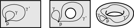
Figure 7: Classes of homotopy. Left : the Euclidean plane. Any loop can be shrunk to a point. The fundamental group reduces to identity. Center : a plane with a hole. $\gamma$ is not homotopic to $\gamma^{\prime}$ . Every homotopy class $h_{n}$ is associated to an integer n : $\gamma\in h_{n}$ if it winds n times round the hole in clockwise direction $(n>0)$, $n<0$ in the anticlockwise direction, $n=0$ if it does not wind. Thus the fundamental group is the infinite cyclic group of integers $\sf\textstyle Z\kern-3.99994ptZ$. Right : a torus ${\mathchoice{\hbox{\raise 3.41666pt\hbox to0.0pt{\kern 1.94447pt\vrule height=3.07497pt\hss}\hbox to0.0pt{\kern 3.05557pt\vrule height=3.41666pt\hss}\hbox{$\displaystyle\rm S$}}}{\hbox{\raise 3.41666pt\hbox to0.0pt{\kern 1.94447pt\vrule height=3.07497pt\hss}\hbox to0.0pt{\kern 3.05557pt\vrule height=3.41666pt\hss}\hbox{$\textstyle\rm S$}}}{\hbox{\raise 2.39166pt\hbox to0.0pt{\kern 1.36113pt\vrule height=2.15248pt\hss}\raise 0.23917pt\hbox to0.0pt{\kern 1.94444pt\vrule height=2.15248pt\hss}\hbox{$\scriptstyle\rm S$}}}{\hbox{\raise 1.70833pt\hbox to0.0pt{\kern 1.11108pt\vrule height=1.53748pt\hss}\raise 0.17084pt\hbox to0.0pt{\kern 1.52779pt\vrule height=1.53748pt\hss}\hbox{$\scriptscriptstyle\rm S$}}}}^{1}\times{\mathchoice{\hbox{\raise 3.41666pt\hbox to0.0pt{\kern 1.94447pt\vrule height=3.07497pt\hss}\hbox to0.0pt{\kern 3.05557pt\vrule height=3.41666pt\hss}\hbox{$\displaystyle\rm S$}}}{\hbox{\raise 3.41666pt\hbox to0.0pt{\kern 1.94447pt\vrule height=3.07497pt\hss}\hbox to0.0pt{\kern 3.05557pt\vrule height=3.41666pt\hss}\hbox{$\textstyle\rm S$}}}{\hbox{\raise 2.39166pt\hbox to0.0pt{\kern 1.36113pt\vrule height=2.15248pt\hss}\raise 0.23917pt\hbox to0.0pt{\kern 1.94444pt\vrule height=2.15248pt\hss}\hbox{$\scriptstyle\rm S$}}}{\hbox{\raise 1.70833pt\hbox to0.0pt{\kern 1.11108pt\vrule height=1.53748pt\hss}\raise 0.17084pt\hbox to0.0pt{\kern 1.52779pt\vrule height=1.53748pt\hss}\hbox{$\scriptscriptstyle\rm S$}}}}^{1}$. Loops can wind m times around the central hole and n times around the body of the torus. Thus the fundamental group consists of pairs $(m,n)$ of integers with addition $(m,n)+(p,q)=(m+p,n+q)$. In other words it is isomorphic to ${\mathchoice{\hbox{$\sf\textstyle Z\kern-3.99994ptZ$}}{\hbox{$\sf\textstyle Z\kern-3.99994ptZ$}}{\hbox{$\sf\scriptstyle Z\kern-2.10002ptZ$}}{\hbox{$\sf\scriptscriptstyle Z\kern-0.99998ptZ$}}}\oplus{\mathchoice{\hbox{$\sf\textstyle Z\kern-3.99994ptZ$}}{\hbox{$\sf\textstyle Z\kern-3.99994ptZ$}}{\hbox{$\sf\scriptstyle Z\kern-2.10002ptZ$}}{\hbox{$\sf\scriptscriptstyle Z\kern-0.99998ptZ$}}}$.

For surfaces, it was shown in the last century that multi–connectedness means that the fundamental group is non trivial : loosely speaking, there is at least one loop that cannot be shrunk to a point. But in higher dimensions the problem is more complex because loops, being only one–dimensional structures, are not sufficient to capture all the topological features of the manifolds. The purpose of algebraic topology, extensively developed during the twentieth century, is to generalise the concept of homotopic loops and to define higher homotopy groups. However the fundamental group (the first homotopy group) remains essential. In 1904, Poincaré [127] had conjectured that any connected closed n–dimensional manifold having a trivial fundamental group must be topologically equivalent to the sphere ${\mathchoice{\hbox{\raise 3.41666pt\hbox to0.0pt{\kern 1.94447pt\vrule height=3.07497pt\hss}\hbox to0.0pt{\kern 3.05557pt\vrule height=3.41666pt\hss}\hbox{$\displaystyle\rm S$}}}{\hbox{\raise 3.41666pt\hbox to0.0pt{\kern 1.94447pt\vrule height=3.07497pt\hss}\hbox to0.0pt{\kern 3.05557pt\vrule height=3.41666pt\hss}\hbox{$\textstyle\rm S$}}}{\hbox{\raise 2.39166pt\hbox to0.0pt{\kern 1.36113pt\vrule height=2.15248pt\hss}\raise 0.23917pt\hbox to0.0pt{\kern 1.94444pt\vrule height=2.15248pt\hss}\hbox{$\scriptstyle\rm S$}}}{\hbox{\raise 1.70833pt\hbox to0.0pt{\kern 1.11108pt\vrule height=1.53748pt\hss}\raise 0.17084pt\hbox to0.0pt{\kern 1.52779pt\vrule height=1.53748pt\hss}\hbox{$\scriptscriptstyle\rm S$}}}}^{n}$. The conjecture was proved by steps during the last 80 years; curiously enough the most difficult case was for n = 3 [130].

3.4.2 Universal Covering Space

The cylinder ${\mathchoice{\hbox{\raise 3.41666pt\hbox to0.0pt{\kern 1.94447pt\vrule height=3.07497pt\hss}\hbox to0.0pt{\kern 3.05557pt\vrule height=3.41666pt\hss}\hbox{$\displaystyle\rm S$}}}{\hbox{\raise 3.41666pt\hbox to0.0pt{\kern 1.94447pt\vrule height=3.07497pt\hss}\hbox to0.0pt{\kern 3.05557pt\vrule height=3.41666pt\hss}\hbox{$\textstyle\rm S$}}}{\hbox{\raise 2.39166pt\hbox to0.0pt{\kern 1.36113pt\vrule height=2.15248pt\hss}\raise 0.23917pt\hbox to0.0pt{\kern 1.94444pt\vrule height=2.15248pt\hss}\hbox{$\scriptstyle\rm S$}}}{\hbox{\raise 1.70833pt\hbox to0.0pt{\kern 1.11108pt\vrule height=1.53748pt\hss}\raise 0.17084pt\hbox to0.0pt{\kern 1.52779pt\vrule height=1.53748pt\hss}\hbox{$\scriptscriptstyle\rm S$}}}}^{1}\times{\rm I\!R}$, embedded in ${\rm I\!R}^{3}$, is a locally Euclidean space whose metric can be written $ds^{2}=R^{2}d\theta^{2}+dz^{2}$. Its geodesics are helices. Any domain $\cal{D}$ bounded by a closed curve that does not intersect all the generatrices of the cylinder is simply-connected. If we unroll once the cylinder on the Euclidean plane ${\rm I\!R}^{2}$, the domain $\cal{D}$ leaves an imprint domain $\Delta$ called its development (figure 8). There is a one-to-one correspondence between the points of $\cal{D}$ and those of $\Delta$, and all the distances remain unchanged. Inside $\cal{D}$, all the properties of Euclidean geometry are valid : the sum of the angles of a triangle is 180 degrees; one and only one geodesic joins two any distinct points; and so on …

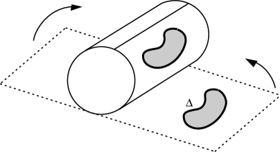
Figure 8: Development of a simply-connected domain of the cylinder.

Now consider the domain $\cal{D^{\prime}}$ bounded by two circular sections of the cylinder (figure 9). $\cal{D^{\prime}}$ is obviously multi–connected because between two arbitrary points $P$ and $P^{\prime}$ can now pass an infinite number of geodesics, which are helices of different pitch. Furthermore, the development $\Delta^{\prime}$ of $\cal{D^{\prime}}$ in the plane ${\rm I\!R}^{2}$ is no more a one–to–one correspondance. If we unroll the cylinder on ${\rm I\!R}^{2}$, every point of $\cal{D^{\prime}}$ generates an infinite number of imprinted points in $\Delta^{\prime}$. Therefore, although the metric properties of Euclidean space remain valid in $\cal{D^{\prime}}$ (such as the value of the sum of the angles of a triangle), the topological properties (such as the unicity of geodesics) do not.

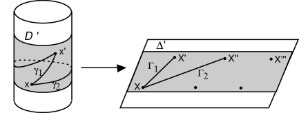
Figure 9: Development of a multi-connected domain of the cylinder.

The development can be extended step by step. A point $\bf x$ and a path $\gamma$ from $\bf x$ to $\bf x^{\prime}$ on the cylinder can be developed into the point $\bf X$ and the path $\Gamma$ from $\bf X$ to $\bf X^{\prime}$ in ${\rm I\!R}^{2}$. $\bf X^{\prime}$ and $\Gamma$ are unique if $\bf x^{\prime}$ and $\gamma$ lie in a simply-connected domain $\cal{D}$ of the cylinder. In the other case, if $\cal{D}$ is multi-connected, there are several paths $\gamma_{1},\gamma_{2},\ldots$ from $\bf x$ to $\bf x^{\prime}$ such that their developments $\Gamma_{1},\Gamma_{2}$ …generate the distinct points ${\bf X^{\prime}},{\bf X^{\prime\prime}}$, …in ${\rm I\!R}^{2}$. The Euclidean plane appears as the Universal Covering Space of the cylinder.

Such a procedure can be generalized to any manifold. Start with a manifold $\cal M$ with metric $\bf g$. Choose a base point x in $\cal M$ and consider the differents paths from x to an other point y. Each path belongs to a homotopy class $\gamma$ of loops at x. We construct the universal covering space as the new manifold ($\widetilde{\cal M}$,$\tilde{\bf g}$) such that each point $\tilde{\bf y}$ of $\widetilde{\cal M}$ is obtained as a pair (${\bf y},\gamma$), y varying over the whole of $\cal M$ while x remains fixed . The metric $\tilde{\bf g}$ is obtained by defining the interval from $\tilde{\bf x}=({\bf x},\gamma)$ to a nearby point $\tilde{\bf x^{\prime}}=({\bf x^{\prime}},\gamma)$ in $\widetilde{\cal M}$ to be equal to the interval from $\bf x$ to $\bf x^{\prime}$ in $\cal M$. By construction, ($\widetilde{\cal M}$,$\tilde{\bf g}$) is locally indistinguishable from (${\cal M},{\bf g}$). But its global – namely topological – properties can be quite different. It is clear that, when $\cal M$ is simply–connected, it is identical to its universal covering space $\widetilde{\cal M}$. When $\cal M$ is multi–connected, each point of $\cal M$ generates an infinite number of points in $\widetilde{\cal M}$. The universal covering space can thus be thought of as an “unwrapping” of the original manifold (see figure 10).

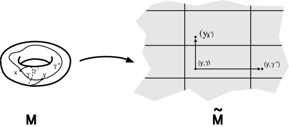
Figure 10: Universal covering space of the torus.

3.4.3 Holonomy group

Consider a point ${\bf x}$ and a loop $\gamma$ at x in $\cal M$. If $\gamma$ lies entirely in a simply-connected domain of $\cal M$, (${\bf x},\gamma$) generates a single point $\tilde{\bf x}$ in $\widetilde{\cal M}$. Otherwise, it generates additional points $\tilde{\bf x^{\prime}},\tilde{\bf x^{\prime\prime}}$, …which are said to be homologous to $\tilde{\bf x}$. The displacements $\tilde{\bf x}\mapsto\tilde{\bf x^{\prime}}$, $\tilde{\bf x}\mapsto\tilde{\bf x^{\prime\prime}}$, …are isometries and form the so-called holonomy group $\Gamma$ in $\widetilde{\cal M}$. This group is discontinuous, i.e., there is a non zero shortest distance between any two homologous points, and the generators of the group (except the identity) have no fixed point. This last property is very restrictive (it excludes for instance the rotations) and allows to classify all the possible groups of holonomy.

Equipped with such properties, the holonomy group is said to act freely and discontinuously on $\widetilde{\cal M}$. The holonomy group is isomorphic to the fundamental group $\pi_{1}(\widetilde{\cal M})$ (see for instance [14]).

3.4.4 Fundamental polyhedron

The geometrical properties of a manifold $\cal M$ within a simply–connected domain are the same as those of its development in the universal covering $\widetilde{\cal M}$. It may be asked what is the largest simply–connected domain containing a given point $x$ of $\cal M$, namely the set $\bigl{\{}y\in{\cal M},d(y,x)\leq d(y,\gamma(x)),\forall\gamma\in\Gamma\bigr{\}}$. Its development in $\widetilde{\cal M}$ is called the fundamental polyhedron ($FP$).

The $FP$ is always convex and has a finite number of faces (due to the fact that the holonomy group is discrete). These faces are homologous by pairs : to every face $\cal F$ corresponds one and only one face $\cal{F^{\prime}}$, such that, for any point ${\bf X}\in~{}{\cal F}$ there exists a point ${\bf X^{\prime}}\in~{}{\cal F^{\prime}}$, which are two developments of the same point $\bf x$ in $\cal M$. The displacements carrying $\cal F$ to $\cal{F^{\prime}}$ are the generators of the holonomy group $\Gamma$.

Note that in dimension 2, the $FP$ is a surface whose boundary is constituted by lines, thus a polygon. In dimension 3, it is a volume bounded by faces, thus a polyhedron.

The configuration formed by the fundamental polyhedron $\cal P$ and its images $\gamma$$\cal P$ ($\gamma\in\Gamma$) is called a tesselation of $\widetilde{\cal M}$, each image $\gamma$$\cal P$ being a cell of the tesselation.

The $FP$ presents two major interests:

• The fundamental group of a given topological manifold $\cal M$ is isomorphic to the fundamental group of the $FP$. Since routine methods are available to determine the holonomy group of as a polyhedron, the problem is considerably simplified.

• The $FP$ allows one to represent any curve in $\cal M$, since any portion of a curve lying outside the $FP$ can be carried inside it by appropriate holonomies (figure 11).

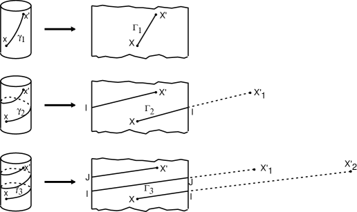
Figure 11: Development of geodesics of the cylinder.

As a general conclusion of this section, the method for classifying the topologies of a given manifold $\cal M$ is :

• to determine its universal covering space $\widetilde{\cal M}$

• to find the fundamental polyhedron $FP$

• to calculate the holonomy group acting on the $FP$.

In sections 4 to 8 this is done for the two– and three–dimensional homogeneous manifolds.

4 Classification of Riemannian surfaces

In addition to pedagogical and illustrative interest, the classification of two–dimensional Riemannian surfaces plays an important role in physics for understanding (2+1)–dimensional gravity, a toy model to gain insight into the real world of (3+1)–dimensional quantum gravity [146, 74, 68, 28, 157, 64]. Also, from a mathematical point of view, three–dimensional spaces can be constructed from surfaces.

As we have seen in section 3.3.3, any Riemannian surface is homeomorphic to a surface admitting a metric with constant curvature k. Thus any Riemannian surface can be expressed as the quotient $\cal{M}$ $=\widetilde{\cal M}/\Gamma$, where the universal covering space $\widetilde{\cal M}$ is either (figure 12) :

• the Euclidean plane ${\rm I\!R}^{2}$ if $k=0$

• the sphere ${\mathchoice{\hbox{\raise 3.41666pt\hbox to0.0pt{\kern 1.94447pt\vrule height=3.07497pt\hss}\hbox to0.0pt{\kern 3.05557pt\vrule height=3.41666pt\hss}\hbox{$\displaystyle\rm S$}}}{\hbox{\raise 3.41666pt\hbox to0.0pt{\kern 1.94447pt\vrule height=3.07497pt\hss}\hbox to0.0pt{\kern 3.05557pt\vrule height=3.41666pt\hss}\hbox{$\textstyle\rm S$}}}{\hbox{\raise 2.39166pt\hbox to0.0pt{\kern 1.36113pt\vrule height=2.15248pt\hss}\raise 0.23917pt\hbox to0.0pt{\kern 1.94444pt\vrule height=2.15248pt\hss}\hbox{$\scriptstyle\rm S$}}}{\hbox{\raise 1.70833pt\hbox to0.0pt{\kern 1.11108pt\vrule height=1.53748pt\hss}\raise 0.17084pt\hbox to0.0pt{\kern 1.52779pt\vrule height=1.53748pt\hss}\hbox{$\scriptscriptstyle\rm S$}}}}^{2}$ if $k>0$

• the hyperbolic plane ${\rm I\!H}^{2}$ if $k<0$.

and $\Gamma$ is a discrete group of isometries without fixed point of $\widetilde{\cal M}$ (figure 12).

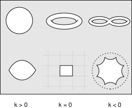
Figure 12: The three kinds of geometries for Riemannian surfaces, with their universal covering space.

To characterise the quotient spaces we adopt the following abbreviations :

C = closed, O = open, SC = simply–connected, MC = multi–connected, OR = orientable, NOR = non-orientable.

4.1 Locally Euclidean surfaces

The UC space is the Euclidean plane ${\rm I\!R}^{2}$ with standard metric $d\sigma^{2}=dx^{2}+dy^{2}$ or, in polar coordinates, $d\sigma^{2}=dr^{2}+r^{2}d\phi^{2}$. The full isometry group of ${\rm I\!R}^{2}$ (the Galilean group) is composed of translations, rotations, reflections and glide reflections (a glide reflection is a translation composed with a reflection in a line parallel to the translation; more pictorially, the correspondance between two successive footprints on a straight snowy path is a glide reflection) .

The subgroups of discrete isometries without fixed point contain only translations and glide reflections. This allows one to classify locally Euclidean surfaces into only 5 types : the simply–connected Euclidean plane itself ${\rm I\!R}$, the multi–connected cylinder ${\rm I\!R}\times{\mathchoice{\hbox{\raise 3.41666pt\hbox to0.0pt{\kern 1.94447pt\vrule height=3.07497pt\hss}\hbox to0.0pt{\kern 3.05557pt\vrule height=3.41666pt\hss}\hbox{$\displaystyle\rm S$}}}{\hbox{\raise 3.41666pt\hbox to0.0pt{\kern 1.94447pt\vrule height=3.07497pt\hss}\hbox to0.0pt{\kern 3.05557pt\vrule height=3.41666pt\hss}\hbox{$\textstyle\rm S$}}}{\hbox{\raise 2.39166pt\hbox to0.0pt{\kern 1.36113pt\vrule height=2.15248pt\hss}\raise 0.23917pt\hbox to0.0pt{\kern 1.94444pt\vrule height=2.15248pt\hss}\hbox{$\scriptstyle\rm S$}}}{\hbox{\raise 1.70833pt\hbox to0.0pt{\kern 1.11108pt\vrule height=1.53748pt\hss}\raise 0.17084pt\hbox to0.0pt{\kern 1.52779pt\vrule height=1.53748pt\hss}\hbox{$\scriptscriptstyle\rm S$}}}}^{1}$, the Möbius band, the torus ${\mathchoice{\hbox{\raise 3.41666pt\hbox to0.0pt{\kern 1.94447pt\vrule height=3.07497pt\hss}\hbox to0.0pt{\kern 3.05557pt\vrule height=3.41666pt\hss}\hbox{$\displaystyle\rm S$}}}{\hbox{\raise 3.41666pt\hbox to0.0pt{\kern 1.94447pt\vrule height=3.07497pt\hss}\hbox to0.0pt{\kern 3.05557pt\vrule height=3.41666pt\hss}\hbox{$\textstyle\rm S$}}}{\hbox{\raise 2.39166pt\hbox to0.0pt{\kern 1.36113pt\vrule height=2.15248pt\hss}\raise 0.23917pt\hbox to0.0pt{\kern 1.94444pt\vrule height=2.15248pt\hss}\hbox{$\scriptstyle\rm S$}}}{\hbox{\raise 1.70833pt\hbox to0.0pt{\kern 1.11108pt\vrule height=1.53748pt\hss}\raise 0.17084pt\hbox to0.0pt{\kern 1.52779pt\vrule height=1.53748pt\hss}\hbox{$\scriptscriptstyle\rm S$}}}}^{1}\times{\mathchoice{\hbox{\raise 3.41666pt\hbox to0.0pt{\kern 1.94447pt\vrule height=3.07497pt\hss}\hbox to0.0pt{\kern 3.05557pt\vrule height=3.41666pt\hss}\hbox{$\displaystyle\rm S$}}}{\hbox{\raise 3.41666pt\hbox to0.0pt{\kern 1.94447pt\vrule height=3.07497pt\hss}\hbox to0.0pt{\kern 3.05557pt\vrule height=3.41666pt\hss}\hbox{$\textstyle\rm S$}}}{\hbox{\raise 2.39166pt\hbox to0.0pt{\kern 1.36113pt\vrule height=2.15248pt\hss}\raise 0.23917pt\hbox to0.0pt{\kern 1.94444pt\vrule height=2.15248pt\hss}\hbox{$\scriptstyle\rm S$}}}{\hbox{\raise 1.70833pt\hbox to0.0pt{\kern 1.11108pt\vrule height=1.53748pt\hss}\raise 0.17084pt\hbox to0.0pt{\kern 1.52779pt\vrule height=1.53748pt\hss}\hbox{$\scriptscriptstyle\rm S$}}}}^{1}$ and the Klein bottle. Their characteristics are summarized in figure 13. It is well known that the Möbius band and the Klein bottle are not orientable. The torus and the Klein bottle are closed spaces. We point out that the projective plane, obtained by identifying the opposite faces of a square under the action of two independent translations, has a strictly positive curvature and is therefore locally spherical.

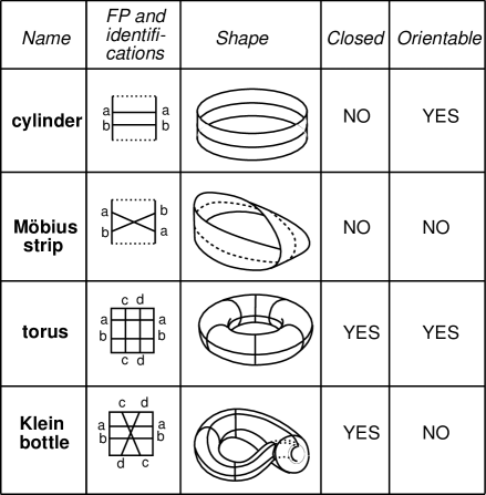
Figure 13: The four types of multi-connected Euclidean surfaces.

4.2 Locally spherical surfaces

The sphere ${\mathchoice{\hbox{\raise 3.41666pt\hbox to0.0pt{\kern 1.94447pt\vrule height=3.07497pt\hss}\hbox to0.0pt{\kern 3.05557pt\vrule height=3.41666pt\hss}\hbox{$\displaystyle\rm S$}}}{\hbox{\raise 3.41666pt\hbox to0.0pt{\kern 1.94447pt\vrule height=3.07497pt\hss}\hbox to0.0pt{\kern 3.05557pt\vrule height=3.41666pt\hss}\hbox{$\textstyle\rm S$}}}{\hbox{\raise 2.39166pt\hbox to0.0pt{\kern 1.36113pt\vrule height=2.15248pt\hss}\raise 0.23917pt\hbox to0.0pt{\kern 1.94444pt\vrule height=2.15248pt\hss}\hbox{$\scriptstyle\rm S$}}}{\hbox{\raise 1.70833pt\hbox to0.0pt{\kern 1.11108pt\vrule height=1.53748pt\hss}\raise 0.17084pt\hbox to0.0pt{\kern 1.52779pt\vrule height=1.53748pt\hss}\hbox{$\scriptscriptstyle\rm S$}}}}^{2}$ admits a homogeneous metric induced from its embedding in ${\rm I\!R}^{3}$, namely the surface of equation $x^{2}+y^{2}+z^{2}=1$. Introducing coordinates $(\theta,\phi)$ by

$$x~{}=~{}sin\theta~{}cos\phi,~{}y~{}=~{}sin\theta~{}sin\phi,~{}z~{}=~{}cos\theta,$$

the induced metric on ${\mathchoice{\hbox{\raise 3.41666pt\hbox to0.0pt{\kern 1.94447pt\vrule height=3.07497pt\hss}\hbox to0.0pt{\kern 3.05557pt\vrule height=3.41666pt\hss}\hbox{$\displaystyle\rm S$}}}{\hbox{\raise 3.41666pt\hbox to0.0pt{\kern 1.94447pt\vrule height=3.07497pt\hss}\hbox to0.0pt{\kern 3.05557pt\vrule height=3.41666pt\hss}\hbox{$\textstyle\rm S$}}}{\hbox{\raise 2.39166pt\hbox to0.0pt{\kern 1.36113pt\vrule height=2.15248pt\hss}\raise 0.23917pt\hbox to0.0pt{\kern 1.94444pt\vrule height=2.15248pt\hss}\hbox{$\scriptstyle\rm S$}}}{\hbox{\raise 1.70833pt\hbox to0.0pt{\kern 1.11108pt\vrule height=1.53748pt\hss}\raise 0.17084pt\hbox to0.0pt{\kern 1.52779pt\vrule height=1.53748pt\hss}\hbox{$\scriptscriptstyle\rm S$}}}}^{2}$ becomes

$$d\sigma^{2}=d\theta^{2}+sin^{2}\theta d\phi^{2}~{}~{}~{}~{}~{}~{}~{}(0\leq\phi\leq 2\pi,~{}0\leq\theta\leq\pi).$$ (12)

The full isometry group of ${\mathchoice{\hbox{\raise 3.41666pt\hbox to0.0pt{\kern 1.94447pt\vrule height=3.07497pt\hss}\hbox to0.0pt{\kern 3.05557pt\vrule height=3.41666pt\hss}\hbox{$\displaystyle\rm S$}}}{\hbox{\raise 3.41666pt\hbox to0.0pt{\kern 1.94447pt\vrule height=3.07497pt\hss}\hbox to0.0pt{\kern 3.05557pt\vrule height=3.41666pt\hss}\hbox{$\textstyle\rm S$}}}{\hbox{\raise 2.39166pt\hbox to0.0pt{\kern 1.36113pt\vrule height=2.15248pt\hss}\raise 0.23917pt\hbox to0.0pt{\kern 1.94444pt\vrule height=2.15248pt\hss}\hbox{$\scriptstyle\rm S$}}}{\hbox{\raise 1.70833pt\hbox to0.0pt{\kern 1.11108pt\vrule height=1.53748pt\hss}\raise 0.17084pt\hbox to0.0pt{\kern 1.52779pt\vrule height=1.53748pt\hss}\hbox{$\scriptscriptstyle\rm S$}}}}^{2}$ is the group of $3\times 3$ orthogonal matrices $O(3)$ (with determinant $\pm 1$). But there is only one non–trivial discrete subgroup without fixed point, namely the group ${\mathchoice{\hbox{$\sf\textstyle Z\kern-3.99994ptZ$}}{\hbox{$\sf\textstyle Z\kern-3.99994ptZ$}}{\hbox{$\sf\scriptstyle Z\kern-2.10002ptZ$}}{\hbox{$\sf\scriptscriptstyle Z\kern-0.99998ptZ$}}}_{2}$, of order two. It is generated by the antipodal map of ${\mathchoice{\hbox{\raise 3.41666pt\hbox to0.0pt{\kern 1.94447pt\vrule height=3.07497pt\hss}\hbox to0.0pt{\kern 3.05557pt\vrule height=3.41666pt\hss}\hbox{$\displaystyle\rm S$}}}{\hbox{\raise 3.41666pt\hbox to0.0pt{\kern 1.94447pt\vrule height=3.07497pt\hss}\hbox to0.0pt{\kern 3.05557pt\vrule height=3.41666pt\hss}\hbox{$\textstyle\rm S$}}}{\hbox{\raise 2.39166pt\hbox to0.0pt{\kern 1.36113pt\vrule height=2.15248pt\hss}\raise 0.23917pt\hbox to0.0pt{\kern 1.94444pt\vrule height=2.15248pt\hss}\hbox{$\scriptstyle\rm S$}}}{\hbox{\raise 1.70833pt\hbox to0.0pt{\kern 1.11108pt\vrule height=1.53748pt\hss}\raise 0.17084pt\hbox to0.0pt{\kern 1.52779pt\vrule height=1.53748pt\hss}\hbox{$\scriptscriptstyle\rm S$}}}}^{2}$ which identifies diametrically opposite points on the surface of the sphere.

As a result there are only two spherical surface forms  :

• the sphere ${\mathchoice{\hbox{\raise 3.41666pt\hbox to0.0pt{\kern 1.94447pt\vrule height=3.07497pt\hss}\hbox to0.0pt{\kern 3.05557pt\vrule height=3.41666pt\hss}\hbox{$\displaystyle\rm S$}}}{\hbox{\raise 3.41666pt\hbox to0.0pt{\kern 1.94447pt\vrule height=3.07497pt\hss}\hbox to0.0pt{\kern 3.05557pt\vrule height=3.41666pt\hss}\hbox{$\textstyle\rm S$}}}{\hbox{\raise 2.39166pt\hbox to0.0pt{\kern 1.36113pt\vrule height=2.15248pt\hss}\raise 0.23917pt\hbox to0.0pt{\kern 1.94444pt\vrule height=2.15248pt\hss}\hbox{$\scriptstyle\rm S$}}}{\hbox{\raise 1.70833pt\hbox to0.0pt{\kern 1.11108pt\vrule height=1.53748pt\hss}\raise 0.17084pt\hbox to0.0pt{\kern 1.52779pt\vrule height=1.53748pt\hss}\hbox{$\scriptscriptstyle\rm S$}}}}^{2}$ iself : C, SC, OR

• the projective plane ${\rm I\!P}^{2}\equiv{\mathchoice{\hbox{\raise 3.41666pt\hbox to0.0pt{\kern 1.94447pt\vrule height=3.07497pt\hss}\hbox to0.0pt{\kern 3.05557pt\vrule height=3.41666pt\hss}\hbox{$\displaystyle\rm S$}}}{\hbox{\raise 3.41666pt\hbox to0.0pt{\kern 1.94447pt\vrule height=3.07497pt\hss}\hbox to0.0pt{\kern 3.05557pt\vrule height=3.41666pt\hss}\hbox{$\textstyle\rm S$}}}{\hbox{\raise 2.39166pt\hbox to0.0pt{\kern 1.36113pt\vrule height=2.15248pt\hss}\raise 0.23917pt\hbox to0.0pt{\kern 1.94444pt\vrule height=2.15248pt\hss}\hbox{$\scriptstyle\rm S$}}}{\hbox{\raise 1.70833pt\hbox to0.0pt{\kern 1.11108pt\vrule height=1.53748pt\hss}\raise 0.17084pt\hbox to0.0pt{\kern 1.52779pt\vrule height=1.53748pt\hss}\hbox{$\scriptscriptstyle\rm S$}}}}^{2}/{\mathchoice{\hbox{$\sf\textstyle Z\kern-3.99994ptZ$}}{\hbox{$\sf\textstyle Z\kern-3.99994ptZ$}}{\hbox{$\sf\scriptstyle Z\kern-2.10002ptZ$}}{\hbox{$\sf\scriptscriptstyle Z\kern-0.99998ptZ$}}}_{2}$ (also called the elliptic plane) : C, MC, NOR.

Whereas the surface of the unit sphere is $4\pi$, the surface of the unit projective plane is only $2\pi$, and its diameter, i.e., the distance between the most widely separated points, only $\pi/2$.

4.3 Locally hyperbolic surfaces

4.3.1 The geometry of ${\rm I\!H}^{2}$

The hyperbolic plane ${\rm I\!H}^{2}$, historically known as the Lobachevski space, is difficult to visualize because it cannot be isometrically imbedded in ${\rm I\!R}^{3}$. Nevertheless it can be thought of as a surface with a saddle point at every point.

Consider the surface of equation $-z^{2}+x^{2}+y^{2}=1$ in the pseudo-Euclidean three-dimensional space with metric $d\sigma^{2}=-dz^{2}+dx^{2}+dy^{2}$ .

If we introduce coordinates $(\chi,\phi)$ by

$$z=cosh\chi,~{}~{}x=sinh\chi~{}cos\phi,~{}~{}y=sinh\chi~{}sin\phi,~{}~{}~{}0\leq\chi<\infty,~{}0\leq\phi\leq 2\pi,$$

the induced metric on ${\rm I\!H}^{2}$ is written as

$$d\sigma^{2}=d\chi^{2}+sinh^{2}\chi~{}d\phi^{2}.$$ (13)

Other representations of ${\rm I\!H}^{2}$ are well-known (figure 14) :

• The upper–half plane $U\equiv\{(x,y)\in{\rm I\!R}^{2},y>0\}$ equipped with the metric

  $$d\sigma^{2}=(dx^{2}+dy^{2})/y^{2},~{}~{}y>0.$$ (14)

  The hyperbolic geodesics correspond to the Euclidean semi-circles, which orthogonally intersect the boundary $\partial U$. The metric (14) is conformally flat, so that the angles between the hyperbolic lines coincide with the Euclidean ones.

• The Poincaré model represents ${\rm I\!H}^{2}$ as the open unit disc $D_{P}\equiv\{(x^{\prime},y^{\prime})\in{\rm I\!R}^{2},~{}x^{\prime 2}+y^{\prime 2}<1\}$. It is obtained from the upper–half space by a coordinate transformation $U\mapsto D_{P}$ which maps $z=x+iy$ into $z^{\prime}=x^{\prime}+iy^{\prime}$ such that $z^{\prime}=-i~{}\frac{z-i}{z+i}$. The metric becomes

  $$d\sigma^{2}=\frac{4~{}dz^{\prime}~{}d\bar{z}^{\prime}}{(1-z^{\prime}\bar{z}^{\prime})^{2}}.$$ (15)

  or, introducing polar coordinates $(r,\phi)$ such that $z^{\prime}=r~{}e^{i\phi}$ :

  $$d\sigma^{2}=\frac{4(dr^{2}+r^{2}d\phi^{2})}{(1-r^{2})^{2}}$$ (16)

  The model is also conformally flat, and the hyperbolic geodesics are mapped onto arcs of circle which meet the frontier of $D_{P}$ at right angles.

• The Klein representation also represents ${\rm I\!H}^{2}$ in an unit open disc $D_{K}\equiv\{(x^{\prime\prime},y^{\prime\prime})\in{\rm I\!R}^{2},x^{2}{}^{\prime\prime}+y^{2}{}^{\prime\prime}<1\}$ with a mapping $D_{P}\mapsto D_{K}$ such that $z^{\prime\prime}\equiv x^{\prime\prime}+iy^{\prime\prime}=\frac{2z^{\prime}}{1+z^{\prime}\bar{z}^{\prime}}$.

  The hyperbolic geodesics are mapped onto Euclidean lines, but this model is not conformally flat.

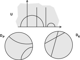
Figure 14: Three representations of ${\rm I\!H}^{2}$ : the upper-half space $U$, the Poincaré model $D_{P}$ and the Klein model $D_{K}$. Representative geodesics are shown.

4.3.2 The holonomies of ${\rm I\!H}^{2}$

The full isometry group of ${\rm I\!H}^{2}$ is $PSL(2,{\rm I\!R})\equiv SL(2,{\rm I\!R})/{\mathchoice{\hbox{$\sf\textstyle Z\kern-3.99994ptZ$}}{\hbox{$\sf\textstyle Z\kern-3.99994ptZ$}}{\hbox{$\sf\scriptstyle Z\kern-2.10002ptZ$}}{\hbox{$\sf\scriptscriptstyle Z\kern-0.99998ptZ$}}}_{2}$, where $SL(2,{\rm I\!R})$ is the group of real $2\times 2$ matrices with unit determinant. In metric (15), any isometry of ${\rm I\!H}^{2}$ can be expressed by a Möbius transformation

$$z\mapsto\frac{az+b}{cz+d}$$

where $z$ is complex, $a,~{}b~{},c~{},d$ real, $ad-bc>0$.

Discrete subgroups without fixed point $\Gamma$ are described for instance in [103]. The topological classification of locally hyperbolic surfaces follows. It is complete only for the compact ${\rm I\!H}^{2}/\Gamma$, which fall into one of the following categories :

• g–torus $T_{g}$, $g\geq 2$ (connected sum of g simple toruses) : C, MC, OR

• connected sum of n projective planes : C, MC, NOR

• connected sum of a compact orientable surface (${\mathchoice{\hbox{\raise 3.41666pt\hbox to0.0pt{\kern 1.94447pt\vrule height=3.07497pt\hss}\hbox to0.0pt{\kern 3.05557pt\vrule height=3.41666pt\hss}\hbox{$\displaystyle\rm S$}}}{\hbox{\raise 3.41666pt\hbox to0.0pt{\kern 1.94447pt\vrule height=3.07497pt\hss}\hbox to0.0pt{\kern 3.05557pt\vrule height=3.41666pt\hss}\hbox{$\textstyle\rm S$}}}{\hbox{\raise 2.39166pt\hbox to0.0pt{\kern 1.36113pt\vrule height=2.15248pt\hss}\raise 0.23917pt\hbox to0.0pt{\kern 1.94444pt\vrule height=2.15248pt\hss}\hbox{$\scriptstyle\rm S$}}}{\hbox{\raise 1.70833pt\hbox to0.0pt{\kern 1.11108pt\vrule height=1.53748pt\hss}\raise 0.17084pt\hbox to0.0pt{\kern 1.52779pt\vrule height=1.53748pt\hss}\hbox{$\scriptscriptstyle\rm S$}}}}^{2}$ or $T_{g}$) and of a projective plane or a Klein bottle : C, MC, NOR

All of these surfaces have a finite area bounded below by $2\pi$, and a diameter greater than $ch^{-1}(4)\approx 2.06$ [10].

In addition, there are an infinite number of non–compact locally hyperbolic surfaces, but their full classification is not achieved. Anyway, it is clear that “almost all” Riemannian surfaces are hyperbolic, since :

- Any open surface other than the Euclidean plane, the cylinder and the Möbius band is homeomorphic to a locally hyperbolic surface, for example an hyperbolic plane with or without handles.

- Any closed surface which is not the sphere, the projective plane, the torus or the Klein bottle is homeomorphic to a locally hyperbolic surface.

4.3.3 Examples

The best known example of a compact hyperbolic surface is the 2-torus $T_{2}$ ( see section 3.2.2). In this case, the FP is a regular octogon with pairs of sides identified. In the Poincaré representation of ${\rm I\!H}^{2}$, the FP appears curvilinear. The pavement of the unit disk by homologous octogons (which appear distorded in this representation) corresponds to the tesselation of ${\rm I\!H}^{2}$ by regular octogons (figure 15). The famous Dutch artist M.–C. Escher [24] has designed fascinating drawings and prints using such tilings of the hyperbolic plane.

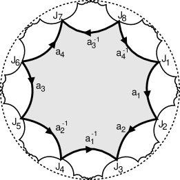
Figure 15: Tesselation of ${\rm I\!H}^{2}$ by octogons in the Poincaré representation. The vertices have the coordinates $z(J_{k})=0.841~{}exp~{}\frac{(3-2k)\pi i}{8}$.

More generally, any compact Riemannian surface $\Sigma_{g}$ with genus $g\geq 2$ can be modelled in ${\rm I\!H}^{2}$. It is representable by the interior of a regular polygon with 4g edges. The length $R$ of an edge is determined by the curvature $k=-1/R^{2}$ of the hyperbolic plane. The angles are $\pi/2g$. The fundamental group is generated by the $2g$ elements $a_{1},a_{2},\ldots,a_{2g}$ such that $a_{1}a_{2}a_{1}^{-1}a_{2}^{-1}\ldots a_{2g-1}a_{2g}a_{2g-1}^{-1}a_{2g}^{-1}=Id$ (figure 15). The Poincaré–Euler characteristic is $\chi(\Sigma_{g})=2(1-g)$. But from Gauss–Bonnet theorem it is also given by $\chi(\Sigma_{g})={1\over{2\pi}}\int\int kd\sigma$. One deduces that the area of the surface is $4\pi(g-1)R^{2}$.

5 Three-dimensional homogeneous spaces

We now consider a three-dimensional Riemannian manifold $\cal M$ admitting at least a 3–dimensional discrete isometry group $\Gamma$ simply transitive on $\cal M$ (cf. section 3.3.3). Such a (locally) homogeneous manifold can be written as the quotient $\widetilde{\cal M}/\Gamma$, where $\widetilde{\cal M}$ is the universal covering space of $\cal M$. Let $G$ be the full group of isometries of $\cal M$ (containing $\Gamma$ as a discrete subgroup). In the terminology used in the theory of classification of compact three–manifolds, $\cal M$ is said to admit a geometric structure modelled on $(\widetilde{\cal M},G)$.

On one hand, Thurston [151] has classified the homogeneous three–dimensional geometries into eight distinct types, generally used by mathematicians.

On the other hand, the Bianchi types are defined from the classification of all simply-transitive 3–dimensional Lie groups . Since the isometries of a Riemannian manifold form a Lie group, the Bianchi classification is used by workers in relativity and cosmology for the description of spatially homogeneous spacetimes [133].

We present below the two approaches and then discuss their mutual relationships [118, 46, 50].

5.1 The Thurston’s eight geometries

Any simply-connected 3–dimensional geometry which admits a compact quotient is equivalent to one of the eight geometries ($\widetilde{\cal M}$$,G$), where $\widetilde{\cal M}$ is ${\rm I\!R}^{3}$, ${\mathchoice{\hbox{\raise 3.41666pt\hbox to0.0pt{\kern 1.94447pt\vrule height=3.07497pt\hss}\hbox to0.0pt{\kern 3.05557pt\vrule height=3.41666pt\hss}\hbox{$\displaystyle\rm S$}}}{\hbox{\raise 3.41666pt\hbox to0.0pt{\kern 1.94447pt\vrule height=3.07497pt\hss}\hbox to0.0pt{\kern 3.05557pt\vrule height=3.41666pt\hss}\hbox{$\textstyle\rm S$}}}{\hbox{\raise 2.39166pt\hbox to0.0pt{\kern 1.36113pt\vrule height=2.15248pt\hss}\raise 0.23917pt\hbox to0.0pt{\kern 1.94444pt\vrule height=2.15248pt\hss}\hbox{$\scriptstyle\rm S$}}}{\hbox{\raise 1.70833pt\hbox to0.0pt{\kern 1.11108pt\vrule height=1.53748pt\hss}\raise 0.17084pt\hbox to0.0pt{\kern 1.52779pt\vrule height=1.53748pt\hss}\hbox{$\scriptscriptstyle\rm S$}}}}^{3}$, ${\rm I\!H}^{3}$, ${\mathchoice{\hbox{\raise 3.41666pt\hbox to0.0pt{\kern 1.94447pt\vrule height=3.07497pt\hss}\hbox to0.0pt{\kern 3.05557pt\vrule height=3.41666pt\hss}\hbox{$\displaystyle\rm S$}}}{\hbox{\raise 3.41666pt\hbox to0.0pt{\kern 1.94447pt\vrule height=3.07497pt\hss}\hbox to0.0pt{\kern 3.05557pt\vrule height=3.41666pt\hss}\hbox{$\textstyle\rm S$}}}{\hbox{\raise 2.39166pt\hbox to0.0pt{\kern 1.36113pt\vrule height=2.15248pt\hss}\raise 0.23917pt\hbox to0.0pt{\kern 1.94444pt\vrule height=2.15248pt\hss}\hbox{$\scriptstyle\rm S$}}}{\hbox{\raise 1.70833pt\hbox to0.0pt{\kern 1.11108pt\vrule height=1.53748pt\hss}\raise 0.17084pt\hbox to0.0pt{\kern 1.52779pt\vrule height=1.53748pt\hss}\hbox{$\scriptscriptstyle\rm S$}}}}^{2}\times{\rm I\!R}$, ${\rm I\!H}^{2}\times{\rm I\!R}$, $\widetilde{SL_{2}{\rm I\!R}}$, $Nil$ or $Sol$, that we shortly describe now (for full details we refer the interested reader to [151, 136]).

• $\widetilde{\cal M}$$={\rm I\!R}^{3}$ : Euclidean geometry

  $G=ISO(3)\equiv R^{3}\times SO(3)$, i.e. the product of the group of translations in ${\rm I\!R}^{3}$ by the group of $3\times 3$ special orthogonal matrices.

  This is the geometry of constant zero curvature. More details are given in section 6

• $\widetilde{\cal M}$$={\mathchoice{\hbox{\raise 3.41666pt\hbox to0.0pt{\kern 1.94447pt\vrule height=3.07497pt\hss}\hbox to0.0pt{\kern 3.05557pt\vrule height=3.41666pt\hss}\hbox{$\displaystyle\rm S$}}}{\hbox{\raise 3.41666pt\hbox to0.0pt{\kern 1.94447pt\vrule height=3.07497pt\hss}\hbox to0.0pt{\kern 3.05557pt\vrule height=3.41666pt\hss}\hbox{$\textstyle\rm S$}}}{\hbox{\raise 2.39166pt\hbox to0.0pt{\kern 1.36113pt\vrule height=2.15248pt\hss}\raise 0.23917pt\hbox to0.0pt{\kern 1.94444pt\vrule height=2.15248pt\hss}\hbox{$\scriptstyle\rm S$}}}{\hbox{\raise 1.70833pt\hbox to0.0pt{\kern 1.11108pt\vrule height=1.53748pt\hss}\raise 0.17084pt\hbox to0.0pt{\kern 1.52779pt\vrule height=1.53748pt\hss}\hbox{$\scriptscriptstyle\rm S$}}}}^{3}$ : spherical geometry

  $G=SO(4)$

  This is the geometry of constant positive curvature. More details are given in section 7.

• $\widetilde{\cal M}$$={\rm I\!H}^{3}$ : hyperbolic geometry

  $G=PSL(2,{\mathchoice{\hbox{\hbox to0.0pt{\kern 2.88884pt\vrule height=6.14993pt\hss}\hbox{$\displaystyle\rm C$}}}{\hbox{\hbox to0.0pt{\kern 2.88884pt\vrule height=6.14993pt\hss}\hbox{$\textstyle\rm C$}}}{\hbox{\hbox to0.0pt{\kern 2.02219pt\vrule height=4.30496pt\hss}\hbox{$\scriptstyle\rm C$}}}{\hbox{\hbox to0.0pt{\kern 1.44441pt\vrule height=3.07497pt\hss}\hbox{$\scriptscriptstyle\rm C$}}}})\equiv SL(2,{\mathchoice{\hbox{\hbox to0.0pt{\kern 2.88884pt\vrule height=6.14993pt\hss}\hbox{$\displaystyle\rm C$}}}{\hbox{\hbox to0.0pt{\kern 2.88884pt\vrule height=6.14993pt\hss}\hbox{$\textstyle\rm C$}}}{\hbox{\hbox to0.0pt{\kern 2.02219pt\vrule height=4.30496pt\hss}\hbox{$\scriptstyle\rm C$}}}{\hbox{\hbox to0.0pt{\kern 1.44441pt\vrule height=3.07497pt\hss}\hbox{$\scriptscriptstyle\rm C$}}}})/{\mathchoice{\hbox{$\sf\textstyle Z\kern-3.99994ptZ$}}{\hbox{$\sf\textstyle Z\kern-3.99994ptZ$}}{\hbox{$\sf\scriptstyle Z\kern-2.10002ptZ$}}{\hbox{$\sf\scriptscriptstyle Z\kern-0.99998ptZ$}}}_{2}$

  This is the geometry of constant negative curvature. More details are given in section 8.

• $\widetilde{\cal M}$$={\mathchoice{\hbox{\raise 3.41666pt\hbox to0.0pt{\kern 1.94447pt\vrule height=3.07497pt\hss}\hbox to0.0pt{\kern 3.05557pt\vrule height=3.41666pt\hss}\hbox{$\displaystyle\rm S$}}}{\hbox{\raise 3.41666pt\hbox to0.0pt{\kern 1.94447pt\vrule height=3.07497pt\hss}\hbox to0.0pt{\kern 3.05557pt\vrule height=3.41666pt\hss}\hbox{$\textstyle\rm S$}}}{\hbox{\raise 2.39166pt\hbox to0.0pt{\kern 1.36113pt\vrule height=2.15248pt\hss}\raise 0.23917pt\hbox to0.0pt{\kern 1.94444pt\vrule height=2.15248pt\hss}\hbox{$\scriptstyle\rm S$}}}{\hbox{\raise 1.70833pt\hbox to0.0pt{\kern 1.11108pt\vrule height=1.53748pt\hss}\raise 0.17084pt\hbox to0.0pt{\kern 1.52779pt\vrule height=1.53748pt\hss}\hbox{$\scriptscriptstyle\rm S$}}}}^{2}\times{\rm I\!R}$

  $G=SO(3)\times{\rm I\!R}$, the products of the corresponding groups.

  The subgroups $\Gamma$ of G acting freely and discontinuously are given by [136]. Only seven 3–manifolds without boundary can be modelled on ${\mathchoice{\hbox{\raise 3.41666pt\hbox to0.0pt{\kern 1.94447pt\vrule height=3.07497pt\hss}\hbox to0.0pt{\kern 3.05557pt\vrule height=3.41666pt\hss}\hbox{$\displaystyle\rm S$}}}{\hbox{\raise 3.41666pt\hbox to0.0pt{\kern 1.94447pt\vrule height=3.07497pt\hss}\hbox to0.0pt{\kern 3.05557pt\vrule height=3.41666pt\hss}\hbox{$\textstyle\rm S$}}}{\hbox{\raise 2.39166pt\hbox to0.0pt{\kern 1.36113pt\vrule height=2.15248pt\hss}\raise 0.23917pt\hbox to0.0pt{\kern 1.94444pt\vrule height=2.15248pt\hss}\hbox{$\scriptstyle\rm S$}}}{\hbox{\raise 1.70833pt\hbox to0.0pt{\kern 1.11108pt\vrule height=1.53748pt\hss}\raise 0.17084pt\hbox to0.0pt{\kern 1.52779pt\vrule height=1.53748pt\hss}\hbox{$\scriptscriptstyle\rm S$}}}}^{2}\times{\rm I\!R}$. Three are non–compact (including ${\mathchoice{\hbox{\raise 3.41666pt\hbox to0.0pt{\kern 1.94447pt\vrule height=3.07497pt\hss}\hbox to0.0pt{\kern 3.05557pt\vrule height=3.41666pt\hss}\hbox{$\displaystyle\rm S$}}}{\hbox{\raise 3.41666pt\hbox to0.0pt{\kern 1.94447pt\vrule height=3.07497pt\hss}\hbox to0.0pt{\kern 3.05557pt\vrule height=3.41666pt\hss}\hbox{$\textstyle\rm S$}}}{\hbox{\raise 2.39166pt\hbox to0.0pt{\kern 1.36113pt\vrule height=2.15248pt\hss}\raise 0.23917pt\hbox to0.0pt{\kern 1.94444pt\vrule height=2.15248pt\hss}\hbox{$\scriptstyle\rm S$}}}{\hbox{\raise 1.70833pt\hbox to0.0pt{\kern 1.11108pt\vrule height=1.53748pt\hss}\raise 0.17084pt\hbox to0.0pt{\kern 1.52779pt\vrule height=1.53748pt\hss}\hbox{$\scriptscriptstyle\rm S$}}}}^{2}\times{\rm I\!R}$ itself), four are compact, including the “three–handle”  ${\mathchoice{\hbox{\raise 3.41666pt\hbox to0.0pt{\kern 1.94447pt\vrule height=3.07497pt\hss}\hbox to0.0pt{\kern 3.05557pt\vrule height=3.41666pt\hss}\hbox{$\displaystyle\rm S$}}}{\hbox{\raise 3.41666pt\hbox to0.0pt{\kern 1.94447pt\vrule height=3.07497pt\hss}\hbox to0.0pt{\kern 3.05557pt\vrule height=3.41666pt\hss}\hbox{$\textstyle\rm S$}}}{\hbox{\raise 2.39166pt\hbox to0.0pt{\kern 1.36113pt\vrule height=2.15248pt\hss}\raise 0.23917pt\hbox to0.0pt{\kern 1.94444pt\vrule height=2.15248pt\hss}\hbox{$\scriptstyle\rm S$}}}{\hbox{\raise 1.70833pt\hbox to0.0pt{\kern 1.11108pt\vrule height=1.53748pt\hss}\raise 0.17084pt\hbox to0.0pt{\kern 1.52779pt\vrule height=1.53748pt\hss}\hbox{$\scriptscriptstyle\rm S$}}}}^{2}\times{\mathchoice{\hbox{\raise 3.41666pt\hbox to0.0pt{\kern 1.94447pt\vrule height=3.07497pt\hss}\hbox to0.0pt{\kern 3.05557pt\vrule height=3.41666pt\hss}\hbox{$\displaystyle\rm S$}}}{\hbox{\raise 3.41666pt\hbox to0.0pt{\kern 1.94447pt\vrule height=3.07497pt\hss}\hbox to0.0pt{\kern 3.05557pt\vrule height=3.41666pt\hss}\hbox{$\textstyle\rm S$}}}{\hbox{\raise 2.39166pt\hbox to0.0pt{\kern 1.36113pt\vrule height=2.15248pt\hss}\raise 0.23917pt\hbox to0.0pt{\kern 1.94444pt\vrule height=2.15248pt\hss}\hbox{$\scriptstyle\rm S$}}}{\hbox{\raise 1.70833pt\hbox to0.0pt{\kern 1.11108pt\vrule height=1.53748pt\hss}\raise 0.17084pt\hbox to0.0pt{\kern 1.52779pt\vrule height=1.53748pt\hss}\hbox{$\scriptscriptstyle\rm S$}}}}^{1}$ [76] and the connected sum of projective spaces ${\rm I\!P}^{3}\oplus{\rm I\!P}^{3}$.

  Metric : $d\sigma^{2}=dr^{2}+sin^{2}rd\phi^{2}+dz^{2}$

• $\widetilde{\cal M}$$={\rm I\!H}^{2}\times{\rm I\!R}$

  $G=PSL(2,{\rm I\!R})\times{\rm I\!R}$, the product of the corresponding groups for ${\rm I\!H}^{2}$ and ${\rm I\!R}$.

  The $\widetilde{\cal M}/\Gamma$ include for instance the product of any compact hyperbolic surface $T_{g}$ (the g–torus or g–handled sphere) with ${\mathchoice{\hbox{\raise 3.41666pt\hbox to0.0pt{\kern 1.94447pt\vrule height=3.07497pt\hss}\hbox to0.0pt{\kern 3.05557pt\vrule height=3.41666pt\hss}\hbox{$\displaystyle\rm S$}}}{\hbox{\raise 3.41666pt\hbox to0.0pt{\kern 1.94447pt\vrule height=3.07497pt\hss}\hbox to0.0pt{\kern 3.05557pt\vrule height=3.41666pt\hss}\hbox{$\textstyle\rm S$}}}{\hbox{\raise 2.39166pt\hbox to0.0pt{\kern 1.36113pt\vrule height=2.15248pt\hss}\raise 0.23917pt\hbox to0.0pt{\kern 1.94444pt\vrule height=2.15248pt\hss}\hbox{$\scriptstyle\rm S$}}}{\hbox{\raise 1.70833pt\hbox to0.0pt{\kern 1.11108pt\vrule height=1.53748pt\hss}\raise 0.17084pt\hbox to0.0pt{\kern 1.52779pt\vrule height=1.53748pt\hss}\hbox{$\scriptscriptstyle\rm S$}}}}^{1}$ or ${\rm I\!R}$ (see the example below).

  Metric : $d\sigma^{2}=dr^{2}+sinh^{2}rd\phi^{2}+dz^{2}$

• $\widetilde{\cal M}$$=\widetilde{SL2{\rm I\!R}}$

  $\widetilde{SL2{\rm I\!R}}$ is the universal covering of $SL(2,{\rm I\!R})$, the 3-dimensional Lie group of all $2\times 2$ real matrices with determinant 1. It is more geometrically described by a fiber bundle whose basis is the hyperbolic plane. Its isometry group is thus the product of translations by $PSL(2,{\rm I\!R}).$

  Metric : $d\sigma^{2}=dx^{2}+cosh^{2}xdy^{2}+(dz+sinhxdy)^{2}$

• $\widetilde{\cal M}$$=Nil$

  $Nil$ is the 3-dimensional Lie group composed of all $3\times 3$ Heisenberg matrices of the form $\left(\begin{array}[]{ccc}1&x&z\\ 0&1&y\\ 0&0&1\end{array}\right)~{}x,y,z\in{\rm I\!R}$. It is more geometrically described by a bundle with the Euclidean plane as base and lines as fibers, or by a bundle with a circle as base and tori as fibers. See [136] for G, which is too complex to be described here.

  Metric :

  $$d\sigma^{2}=dx^{2}+dy^{2}+(dz-xdy)^{2}$$

• $\widetilde{\cal M}$$=Sol$

  $Sol$ is a Lie group which can be represented by ${\rm I\!R}^{3}$ with the multiplication law

  $$(x,y,z)(x^{\prime},y^{\prime},z^{\prime})=(x+e^{-z}x^{\prime},y+e^{z}y^{\prime},z+z^{\prime}).$$

  It is more geometrically described by a bundle over one–dimensional base and two–dimensional fibers. See [136] for G.

  Metric : $d\sigma^{2}=e^{2z}dx^{2}+e^{-2z}dy^{2}+dz^{2}$

Thus, in addition to the three geometries of constant curvature ${\rm I\!R}^{3}$, ${\mathchoice{\hbox{\raise 3.41666pt\hbox to0.0pt{\kern 1.94447pt\vrule height=3.07497pt\hss}\hbox to0.0pt{\kern 3.05557pt\vrule height=3.41666pt\hss}\hbox{$\displaystyle\rm S$}}}{\hbox{\raise 3.41666pt\hbox to0.0pt{\kern 1.94447pt\vrule height=3.07497pt\hss}\hbox to0.0pt{\kern 3.05557pt\vrule height=3.41666pt\hss}\hbox{$\textstyle\rm S$}}}{\hbox{\raise 2.39166pt\hbox to0.0pt{\kern 1.36113pt\vrule height=2.15248pt\hss}\raise 0.23917pt\hbox to0.0pt{\kern 1.94444pt\vrule height=2.15248pt\hss}\hbox{$\scriptstyle\rm S$}}}{\hbox{\raise 1.70833pt\hbox to0.0pt{\kern 1.11108pt\vrule height=1.53748pt\hss}\raise 0.17084pt\hbox to0.0pt{\kern 1.52779pt\vrule height=1.53748pt\hss}\hbox{$\scriptscriptstyle\rm S$}}}}^{3}$ and ${\rm I\!H}^{3}$, there exist five additional homogeneous geometries. In the three first types, $dim(G)=6$ and we have the spaces of constant curvature. In the other types (except $Sol$), $dim(G)=4$ and the corresponding spaces are called locally rotational symmetric.

5.2 Bianchi types

The original work of Bianchi [12] was improved by theoretical cosmologists [41, 38], because of some redundancy between types. For a three-dimensional Lie group, let $\{\xi_{i}\}_{i=1,2,3}$ be a basis of infinitesimal generators, called Killing vectors. The commutation relations $[\xi_{i},\xi_{j}]=C^{k}_{ij}~{}\xi_{k}$ define the structure constants of the Lie group $C^{k}_{ij}$, which fully characterize its algebraic structure. The classification of 3–dimensional Lie groups involves the following decomposition of $C^{k}_{ij}$ :

$$C^{k}_{ij}=\varepsilon_{lij}N^{kl}+\delta^{k}_{j}A_{i}-\delta^{k}_{i}A_{j}$$ (17)

where $\delta^{k}_{ij}$ is the Kronecker symbol and $\varepsilon_{lij}$ the completely antisymmetric form with $\varepsilon_{123}=1$. The Jacobi identity yields $N^{jk}A_{k}=0$. By a change of basis, $N^{jk}$ can be reduced to the diagonal form $(N_{1},N_{2},N_{3})$ with each $N_{i}=\pm 1,0$ and $A_{i}=(a,0,0)$. It follows a natural division into two large classes :

• class A : $a=0$

• class B : $a\neq 0$

The table 1 shows the resulting Bianchi–Behr types.

Table 1: The Bianchi-Behr classification of groups

class	type		N		a
	I	0	0	0	0
	II	1	0	0	0
A	VI0	0	1	-1	0
	VII0	0	1	1	0
	VIII	1	1	-1	0
	IX	1	1	1	0
	V	0	0	0	1
	IV	0	0	1	1
B	VIa, $a<0$	0	1	-1	$\sqrt{-a}$
	(III=VI-1)
	VIIa, $a>0$	0	1	1	$\sqrt{a}$

These groups may also be characterized by invariant bases of 1–forms $\{\omega^{j}\}$, in terms of which the “standard” metric of a given Bianchi type is written as:

$$d\tilde{\sigma}^{2}=(\omega^{1})^{2}+(\omega^{2})^{2}+(\omega^{3})^{2}.$$ (18)

Now the most general Riemannian space invariant under a Bianchi group ( thus called a Bianchi space) has a metric

$$d\sigma^{2}=\gamma_{ab}~{}\omega^{a}\omega^{b},$$ (19)

where the symmetrical coefficients $\gamma_{ab}$ are constant.

Finally, any spacetime with metric

$$ds^{2}=dt^{2}-\gamma_{ab}(t)~{}\omega^{a}\omega^{b}$$ (20)

admits a Bianchi group acting transitively on its spacelike sections. According to our definitions, it is thus a spatially homogeneous universe model.

The Bianchi type $I$ spaces have a group isomorphic to the 3–dimensional translation group of the Euclidean space. They include locally Euclidean spaces. The flat FL (Einstein-de Sitter) spacetime model is invariant under a simply transitive group of type $I$ (defining the spatial homogeneity) and also an isotropy group of type $VII_{0}$. The very-well studied Kasner spacetime [90, 133] has only a simply–transitive isometry group $G_{3}$ of type $I$. It is therefore homogeneous but anisotropic. Its metric is written as  :

$$ds^{2}=dt^{2}-t^{2p_{1}}~{}dx^{2}+t^{2p_{2}}~{}dy^{2}+t^{2p_{3}}~{}dz^{2},$$ (21)

with the $p_{i}$ are constants satisfying $p_{1}+p_{2}+p_{3}=(p_{1})^{2}+(p_{2})^{2}+(p_{3})^{2}=1$. Each hypersurface $\{t=constant\}$ of the Kasner spacetime is a flat three-dimensional space, but the spacetime expands anisotropically.

The Bianchi type $V$ contains locally hyperbolic spaces. The hyperbolic ($k=-1$) FL model is invariant under a simply transitive group of type $V$ (spatial homogeneity) and also an isotropy group of type $VII_{a}$.

The Bianchi type $IX$ has a group isomorphic to the 3–dimensional rotation group SO(3). It therefore contains locally spherical spaces. The spherical ($k=+1$) FL model is invariant under a simply transitive group of type $IX$ (spatial homogeneity) and also an isotropy group of type $IX$ also. The anisotropic “mixmaster” universe [110, 8] has only a simply-transitive isometry group $G_{3}$ of type $IX$.

5.3 Correspondance between Thurston’s geometries and BKS types

One one hand, all the homogeneous 3–dimensional metrics are described by the Bianchi metrics (19) and the additional Kantowski–Sachs metric

$$d\sigma^{2}=a^{2}dx^{2}+b^{2}(dy^{2}+sin^{2}ydz^{2}),$$ (22)

for which the isometry group has dimension 4 and is multiply transitive on 3–dimensional spaces (cf. §3.3.3). They are called collectively BKS metrics.

On the other hand, if a closed 3-space $\cal M$ (not necessarily homogeneous) admits a given BKS metric, then it possesses a geometric structure modelled on $(\widetilde{\cal M},G)$, where $\widetilde{\cal M}$ is the universal covering space and $G$ the corresponding BKS group.

This allows to establish a correspondance between the Thurston’s geometries described in §5.1 and the Bianchi-Kantowski-Sachs types, summarized in Table 2.

Table 2: Relation between Thurston’s geometries and BKS types

Thurston’s geometries	BKS types	class	sectional curvature
${\rm I\!R}^{3}$	I,  VII0	A	$0,0,0$
${\mathchoice{\hbox{\raise 3.41666pt\hbox to0.0pt{\kern 1.94447pt\vrule height=3.07497pt\hss}\hbox to0.0pt{\kern 3.05557pt\vrule height=3.41666pt\hss}\hbox{$\displaystyle\rm S$}}}{\hbox{\raise 3.41666pt\hbox to0.0pt{\kern 1.94447pt\vrule height=3.07497pt\hss}\hbox to0.0pt{\kern 3.05557pt\vrule height=3.41666pt\hss}\hbox{$\textstyle\rm S$}}}{\hbox{\raise 2.39166pt\hbox to0.0pt{\kern 1.36113pt\vrule height=2.15248pt\hss}\raise 0.23917pt\hbox to0.0pt{\kern 1.94444pt\vrule height=2.15248pt\hss}\hbox{$\scriptstyle\rm S$}}}{\hbox{\raise 1.70833pt\hbox to0.0pt{\kern 1.11108pt\vrule height=1.53748pt\hss}\raise 0.17084pt\hbox to0.0pt{\kern 1.52779pt\vrule height=1.53748pt\hss}\hbox{$\scriptscriptstyle\rm S$}}}}^{3}$	IX	A	$1,1,1$
${\rm I\!H}^{3}$	V	B	$-1,-1,-1$
	VIIa, $a>0$		$-a^{2},-a^{2},-a^{2}$
${\mathchoice{\hbox{\raise 3.41666pt\hbox to0.0pt{\kern 1.94447pt\vrule height=3.07497pt\hss}\hbox to0.0pt{\kern 3.05557pt\vrule height=3.41666pt\hss}\hbox{$\displaystyle\rm S$}}}{\hbox{\raise 3.41666pt\hbox to0.0pt{\kern 1.94447pt\vrule height=3.07497pt\hss}\hbox to0.0pt{\kern 3.05557pt\vrule height=3.41666pt\hss}\hbox{$\textstyle\rm S$}}}{\hbox{\raise 2.39166pt\hbox to0.0pt{\kern 1.36113pt\vrule height=2.15248pt\hss}\raise 0.23917pt\hbox to0.0pt{\kern 1.94444pt\vrule height=2.15248pt\hss}\hbox{$\scriptstyle\rm S$}}}{\hbox{\raise 1.70833pt\hbox to0.0pt{\kern 1.11108pt\vrule height=1.53748pt\hss}\raise 0.17084pt\hbox to0.0pt{\kern 1.52779pt\vrule height=1.53748pt\hss}\hbox{$\scriptscriptstyle\rm S$}}}}^{2}\times{\rm I\!R}$	K.S.		$1,0,0$
${\rm I\!H}^{2}\times{\rm I\!R}$	III=VI-1	B	$-1,0,0$
$\widetilde{SL2{\rm I\!R}}$	VIII	A	$-{5\over 4}$,$-{1\over 4}$,$-{1\over 4}$
$Nil$	II	A	$-{1\over 4},{1\over 4},{1\over 4}$
$Sol$	VI0	A	$1,-1,-1$

The following remarks must be done.

• Within the Bianchi types ($I$, $V$, $VII_{a}$, $IX$) admitting a constant curvature space as universal covering, spaces are generally anisotropic. More generally, within a given type, the change of topology obtained by quotienting the universal covering space by $\Gamma$ lowers the dimension of the full group of isometries, because the isotropy group is broken  . A theorem [91] states that the only three–dimensional Riemannian spaces having the full six-dimensional group of isometries are ${\rm I\!R}^{3},~{}{\mathchoice{\hbox{\raise 3.41666pt\hbox to0.0pt{\kern 1.94447pt\vrule height=3.07497pt\hss}\hbox to0.0pt{\kern 3.05557pt\vrule height=3.41666pt\hss}\hbox{$\displaystyle\rm S$}}}{\hbox{\raise 3.41666pt\hbox to0.0pt{\kern 1.94447pt\vrule height=3.07497pt\hss}\hbox to0.0pt{\kern 3.05557pt\vrule height=3.41666pt\hss}\hbox{$\textstyle\rm S$}}}{\hbox{\raise 2.39166pt\hbox to0.0pt{\kern 1.36113pt\vrule height=2.15248pt\hss}\raise 0.23917pt\hbox to0.0pt{\kern 1.94444pt\vrule height=2.15248pt\hss}\hbox{$\scriptstyle\rm S$}}}{\hbox{\raise 1.70833pt\hbox to0.0pt{\kern 1.11108pt\vrule height=1.53748pt\hss}\raise 0.17084pt\hbox to0.0pt{\kern 1.52779pt\vrule height=1.53748pt\hss}\hbox{$\scriptscriptstyle\rm S$}}}}^{3},~{}{\rm I\!P}^{3}$ and ${\rm I\!H}^{3}$. Thus, whereas the universal covering spaces and the projective space are globally isotropic, the quotient spaces are only locally isotropic [35, 144].

• The Bianchi types $IV$ and $VI_{a}~{}(a\neq 0,1)$ are not in correspondance with Thurston’s geometries because they do not admit closed spaces. This may be related to the fact that their sectional curvatures are all different from each other : $\Bigl{(}-3/4,(-5+{2\over\sqrt{5}})/4,(-5-{2\over\sqrt{5}})/4\Bigr{)}$ for type $IV$, $\Bigl{(}1-a^{2},-(1+a)^{2},-(1-a)^{2}\Bigr{)}$ for type $VI_{a}$, but this conjecture remains to be proved.

• From a geometrical point of view, two spacetimes solutions of Einstein’s equations are regarded as physically indistinguishable if they are isometric. Ashtekar and Samuel [4] have however emphasized that this may no more be the case in the the hamiltonian formulation of general relativity, in which the field equations are derived from the Einstein action $I=\int R~{}\sqrt{-g}~{}d^{4}x$. In the case of spatially homogeneous spacetimes, it was already known [100] that the hamiltonian description was available for Bianchi class A and Kantowski-Sachs space-times, but failed for Bianchi class B (for a review, see [134, 133]). Ashtekar and Samuel [4] have proved that the Lie groups underlying all class B spacetimes are merely incompatible with a compact spatial topology, a result previously pointed out in [37]. This can be surprising since we have seen that, for instance, locally hyperbolic 3–manifolds (corresponding to class B types $V$ and $VII_{a}$) do admit compact topologies. But the hamiltonian picture of general relativity further constrains the 4–dimensional metrics (20), and thus imposes additional restrictions on the topology of the spacelike sections. This result unveils an unexpected link between the metric and the topology through the Einstein’s field equations, which should play an essential role in the minisuperspace approach to quantum cosmology [111].

5.4 Example : a quasi-hyperbolic compact space

Fagundes [43, 46] presented a “quasi–hyperbolic” compact space of the form $\Sigma=T_{g}\times{\mathchoice{\hbox{\raise 3.41666pt\hbox to0.0pt{\kern 1.94447pt\vrule height=3.07497pt\hss}\hbox to0.0pt{\kern 3.05557pt\vrule height=3.41666pt\hss}\hbox{$\displaystyle\rm S$}}}{\hbox{\raise 3.41666pt\hbox to0.0pt{\kern 1.94447pt\vrule height=3.07497pt\hss}\hbox to0.0pt{\kern 3.05557pt\vrule height=3.41666pt\hss}\hbox{$\textstyle\rm S$}}}{\hbox{\raise 2.39166pt\hbox to0.0pt{\kern 1.36113pt\vrule height=2.15248pt\hss}\raise 0.23917pt\hbox to0.0pt{\kern 1.94444pt\vrule height=2.15248pt\hss}\hbox{$\scriptstyle\rm S$}}}{\hbox{\raise 1.70833pt\hbox to0.0pt{\kern 1.11108pt\vrule height=1.53748pt\hss}\raise 0.17084pt\hbox to0.0pt{\kern 1.52779pt\vrule height=1.53748pt\hss}\hbox{$\scriptscriptstyle\rm S$}}}}^{1}$, with ${\rm I\!H}^{2}\times{\rm I\!R}$ as universal covering. It is thus a homogeneous anisotropic model. The g–torus $T_{g}$ with hyperbolic 2–metric is parametrized by the coordinates $\rho$ and $\phi$, the circle ${\mathchoice{\hbox{\raise 3.41666pt\hbox to0.0pt{\kern 1.94447pt\vrule height=3.07497pt\hss}\hbox to0.0pt{\kern 3.05557pt\vrule height=3.41666pt\hss}\hbox{$\displaystyle\rm S$}}}{\hbox{\raise 3.41666pt\hbox to0.0pt{\kern 1.94447pt\vrule height=3.07497pt\hss}\hbox to0.0pt{\kern 3.05557pt\vrule height=3.41666pt\hss}\hbox{$\textstyle\rm S$}}}{\hbox{\raise 2.39166pt\hbox to0.0pt{\kern 1.36113pt\vrule height=2.15248pt\hss}\raise 0.23917pt\hbox to0.0pt{\kern 1.94444pt\vrule height=2.15248pt\hss}\hbox{$\scriptstyle\rm S$}}}{\hbox{\raise 1.70833pt\hbox to0.0pt{\kern 1.11108pt\vrule height=1.53748pt\hss}\raise 0.17084pt\hbox to0.0pt{\kern 1.52779pt\vrule height=1.53748pt\hss}\hbox{$\scriptscriptstyle\rm S$}}}}^{1}$ is parametrized by the coordinate $\zeta$.

For a better understanding the figure 16 depicts a “horizontal section” $T_{g}$ of $\Sigma$. The edges of the 4g–gon have a length $\mid a_{i}\mid=2a~{}cosh^{-1}(cot\pi/4g)$, and $\Sigma$ is described by the metric:

$$d\sigma^{2}=b^{2}~{}d\zeta^{2}+a^{2}~{}(d\rho^{2}+sinh^{2}\rho~{}d\phi^{2}),~{}~{}a,b~{}constants.$$ (23)

The range of coordinates is $-\lambda<\zeta<\lambda$ ($\lambda$ = const.), $0<\phi<2\pi$, $0<\rho<\rho_{i}$.

The volume of $\Sigma$ is $V=8\pi g\lambda(g-1)a^{2}b$. The anisotropy of $\Sigma$ is manifest in the horizontal section : from the point of view of $M_{i}$, the points $C$ and $J$ have opposite images at distance $\mid a_{i}\mid/2$, whereas from the point of view of $C$ only the $M_{i}$ provide opposite images at this distance.

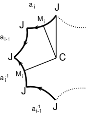
Figure 16: The quasi-hyperbolic model of Fagundes. The edges of the 4g-gon are identified by pairs, so that the two $M_{i}$ are the same, and all the 4g points J are the same. Resolution of the triangle $CJM_{i}$ gives $CM_{i}=a~{}cosh^{-1}(cot\pi/4g)$, $CJ=a~{}cosh^{-1}(cot^{2}\pi/4g)$.

5.5 Spaces of constant curvature

We emphasize that the preceding example was not a space of constant curvature. Cosmology, however, focuses mainly on locally homogeneous and isotropic spaces, namely those admitting one of the 3 geometries of constant curvature. Any compact 3–manifold $\cal{M}$ with constant curvature $k$ can be expressed as the quotient ${\cal M}~{}\equiv~{}\widetilde{\cal M}/\Gamma$, where the Universal Covering space $\widetilde{\cal M}$ is either :

• the Euclidean space ${\rm I\!R}^{3}$ if $k=0$

• the 3-sphere ${\mathchoice{\hbox{\raise 3.41666pt\hbox to0.0pt{\kern 1.94447pt\vrule height=3.07497pt\hss}\hbox to0.0pt{\kern 3.05557pt\vrule height=3.41666pt\hss}\hbox{$\displaystyle\rm S$}}}{\hbox{\raise 3.41666pt\hbox to0.0pt{\kern 1.94447pt\vrule height=3.07497pt\hss}\hbox to0.0pt{\kern 3.05557pt\vrule height=3.41666pt\hss}\hbox{$\textstyle\rm S$}}}{\hbox{\raise 2.39166pt\hbox to0.0pt{\kern 1.36113pt\vrule height=2.15248pt\hss}\raise 0.23917pt\hbox to0.0pt{\kern 1.94444pt\vrule height=2.15248pt\hss}\hbox{$\scriptstyle\rm S$}}}{\hbox{\raise 1.70833pt\hbox to0.0pt{\kern 1.11108pt\vrule height=1.53748pt\hss}\raise 0.17084pt\hbox to0.0pt{\kern 1.52779pt\vrule height=1.53748pt\hss}\hbox{$\scriptscriptstyle\rm S$}}}}^{3}$ if $k>0$

• the hyperbolic 3-space ${\rm I\!H}^{3}$ if $k<0$.

and $\Gamma$ is a subgroup of isometries of $\widetilde{\cal M}$ acting freely and discontinuously. The three following sections are devoted to a more detailed description of such spaces.

6 Three-dimensional Euclidean space forms

The line element for the universal covering space ${\rm I\!R}^{3}$ may be written as :

$$d\sigma^{2}=R^{2}\{d\chi^{2}+\chi^{2}(d\theta^{2}+sin^{2}\theta d\phi^{2})\}$$ (24)

Its full isometry group is $G=ISO(3)\equiv{\rm I\!R}^{3}\times SO(3)$, and the generators of the possible holonomy groups $\Gamma$ (i.e., discrete subgroups without fixed point) include the identity, the translations, the glide reflections and the helicoidal motions occurring in various combinations. They generate 18 distinct types of locally Euclidean spaces [158, 35, 3]. The 17 multi–connected space forms are in correspondance with the 17 cristallographic groups discovered more than a century ago by Fedorov [58]. Eight forms are open (non compact), ten are closed (compact).

6.1 Open models

When $\Gamma$ does not include glide reflections, the space forms ${\rm I\!R}^{3}/\Gamma$ are orientable. They are four :

• type $\cal E$.

  $\Gamma$ reduces to the identity, $\cal M$$\equiv{\rm I\!R}^{3}$.

• type $\cal J$_θ

  $\Gamma$ is generated by an helicoidal motion by an angle $\theta$, $\cal M$ is the topological product of a cylinder by ${\rm I\!R}$.

• type $\cal T$₁

  $\Gamma$ is generated by two independant translations, $\cal M$ is the product of a torus by ${\rm I\!R}$.

• type $\cal K$₁

  $\Gamma$ includes a translation and an helicoidal motion of angle $\pi$ along a direction orthogonal to the translation.

When $\Gamma$ includes a glide reflection, the space forms ${\rm I\!R}^{3}/\Gamma$ are not orientable. We shall not describe them because of their lack of interest for cosmology (cf. section 2)

6.2 Closed models

The compact models can be better visualised by identifying appropriate faces of fundamental polyhedra. Six of them are orientable (figure 17)

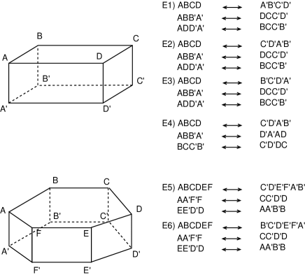
Figure 17: The six locally Euclidean, closed, oriented 3-spaces

The fundamental polyhedron can be a parallelepiped. The possible identifications are then :

• $E_{1}$ - opposite faces by translations. The hypertorus $T^{3}$ already mentioned in section 3.2.3, which is homeomorphic to the topological product ${\mathchoice{\hbox{\raise 3.41666pt\hbox to0.0pt{\kern 1.94447pt\vrule height=3.07497pt\hss}\hbox to0.0pt{\kern 3.05557pt\vrule height=3.41666pt\hss}\hbox{$\displaystyle\rm S$}}}{\hbox{\raise 3.41666pt\hbox to0.0pt{\kern 1.94447pt\vrule height=3.07497pt\hss}\hbox to0.0pt{\kern 3.05557pt\vrule height=3.41666pt\hss}\hbox{$\textstyle\rm S$}}}{\hbox{\raise 2.39166pt\hbox to0.0pt{\kern 1.36113pt\vrule height=2.15248pt\hss}\raise 0.23917pt\hbox to0.0pt{\kern 1.94444pt\vrule height=2.15248pt\hss}\hbox{$\scriptstyle\rm S$}}}{\hbox{\raise 1.70833pt\hbox to0.0pt{\kern 1.11108pt\vrule height=1.53748pt\hss}\raise 0.17084pt\hbox to0.0pt{\kern 1.52779pt\vrule height=1.53748pt\hss}\hbox{$\scriptscriptstyle\rm S$}}}}^{1}\times{\mathchoice{\hbox{\raise 3.41666pt\hbox to0.0pt{\kern 1.94447pt\vrule height=3.07497pt\hss}\hbox to0.0pt{\kern 3.05557pt\vrule height=3.41666pt\hss}\hbox{$\displaystyle\rm S$}}}{\hbox{\raise 3.41666pt\hbox to0.0pt{\kern 1.94447pt\vrule height=3.07497pt\hss}\hbox to0.0pt{\kern 3.05557pt\vrule height=3.41666pt\hss}\hbox{$\textstyle\rm S$}}}{\hbox{\raise 2.39166pt\hbox to0.0pt{\kern 1.36113pt\vrule height=2.15248pt\hss}\raise 0.23917pt\hbox to0.0pt{\kern 1.94444pt\vrule height=2.15248pt\hss}\hbox{$\scriptstyle\rm S$}}}{\hbox{\raise 1.70833pt\hbox to0.0pt{\kern 1.11108pt\vrule height=1.53748pt\hss}\raise 0.17084pt\hbox to0.0pt{\kern 1.52779pt\vrule height=1.53748pt\hss}\hbox{$\scriptscriptstyle\rm S$}}}}^{1}\times{\mathchoice{\hbox{\raise 3.41666pt\hbox to0.0pt{\kern 1.94447pt\vrule height=3.07497pt\hss}\hbox to0.0pt{\kern 3.05557pt\vrule height=3.41666pt\hss}\hbox{$\displaystyle\rm S$}}}{\hbox{\raise 3.41666pt\hbox to0.0pt{\kern 1.94447pt\vrule height=3.07497pt\hss}\hbox to0.0pt{\kern 3.05557pt\vrule height=3.41666pt\hss}\hbox{$\textstyle\rm S$}}}{\hbox{\raise 2.39166pt\hbox to0.0pt{\kern 1.36113pt\vrule height=2.15248pt\hss}\raise 0.23917pt\hbox to0.0pt{\kern 1.94444pt\vrule height=2.15248pt\hss}\hbox{$\scriptstyle\rm S$}}}{\hbox{\raise 1.70833pt\hbox to0.0pt{\kern 1.11108pt\vrule height=1.53748pt\hss}\raise 0.17084pt\hbox to0.0pt{\kern 1.52779pt\vrule height=1.53748pt\hss}\hbox{$\scriptscriptstyle\rm S$}}}}^{1}$, belongs to this class and, due to its simplicity, will provide a preferred field of investigation in the second part of this article.

• $E_{2}$ - opposite faces, one pair being rotated by angle $\pi$

• $E_{3}$ - opposite faces, one pair being rotated by $\pi/2$

• $E_{4}$ - opposite faces, all three pairs being rotated by $\pi$.

The fundamental polyhedron can also be the interior of an hexagonal prism, with two possible identifications :

• $E_{5}$ - opposite faces, the top face being rotated by an angle $2\pi/3$ with respect to the bottom face

• $E_{6}$ - opposite faces, the top face being rotated by an angle $\pi/3$ with respect to the bottom face.

Finally, four spaces are not orientable and we shall not describe them because of their lack of interest for cosmology (cf. section 2).

7 Three-dimensional spherical space forms

Three–manifolds of constant positive curvature were classified by Seifert and Threlfall [137]. Their universal covering being the compact ${\mathchoice{\hbox{\raise 3.41666pt\hbox to0.0pt{\kern 1.94447pt\vrule height=3.07497pt\hss}\hbox to0.0pt{\kern 3.05557pt\vrule height=3.41666pt\hss}\hbox{$\displaystyle\rm S$}}}{\hbox{\raise 3.41666pt\hbox to0.0pt{\kern 1.94447pt\vrule height=3.07497pt\hss}\hbox to0.0pt{\kern 3.05557pt\vrule height=3.41666pt\hss}\hbox{$\textstyle\rm S$}}}{\hbox{\raise 2.39166pt\hbox to0.0pt{\kern 1.36113pt\vrule height=2.15248pt\hss}\raise 0.23917pt\hbox to0.0pt{\kern 1.94444pt\vrule height=2.15248pt\hss}\hbox{$\scriptstyle\rm S$}}}{\hbox{\raise 1.70833pt\hbox to0.0pt{\kern 1.11108pt\vrule height=1.53748pt\hss}\raise 0.17084pt\hbox to0.0pt{\kern 1.52779pt\vrule height=1.53748pt\hss}\hbox{$\scriptscriptstyle\rm S$}}}}^{3}$, they are necessarily compact.

7.1 The geometry of ${\mathchoice{\hbox{\raise 3.41666pt\hbox to0.0pt{\kern 1.94447pt\vrule height=3.07497pt\hss}\hbox to0.0pt{\kern 3.05557pt\vrule height=3.41666pt\hss}\hbox{$\displaystyle\rm S$}}}{\hbox{\raise 3.41666pt\hbox to0.0pt{\kern 1.94447pt\vrule height=3.07497pt\hss}\hbox to0.0pt{\kern 3.05557pt\vrule height=3.41666pt\hss}\hbox{$\textstyle\rm S$}}}{\hbox{\raise 2.39166pt\hbox to0.0pt{\kern 1.36113pt\vrule height=2.15248pt\hss}\raise 0.23917pt\hbox to0.0pt{\kern 1.94444pt\vrule height=2.15248pt\hss}\hbox{$\scriptstyle\rm S$}}}{\hbox{\raise 1.70833pt\hbox to0.0pt{\kern 1.11108pt\vrule height=1.53748pt\hss}\raise 0.17084pt\hbox to0.0pt{\kern 1.52779pt\vrule height=1.53748pt\hss}\hbox{$\scriptscriptstyle\rm S$}}}}^{3}$

The 3–sphere ${\mathchoice{\hbox{\raise 3.41666pt\hbox to0.0pt{\kern 1.94447pt\vrule height=3.07497pt\hss}\hbox to0.0pt{\kern 3.05557pt\vrule height=3.41666pt\hss}\hbox{$\displaystyle\rm S$}}}{\hbox{\raise 3.41666pt\hbox to0.0pt{\kern 1.94447pt\vrule height=3.07497pt\hss}\hbox to0.0pt{\kern 3.05557pt\vrule height=3.41666pt\hss}\hbox{$\textstyle\rm S$}}}{\hbox{\raise 2.39166pt\hbox to0.0pt{\kern 1.36113pt\vrule height=2.15248pt\hss}\raise 0.23917pt\hbox to0.0pt{\kern 1.94444pt\vrule height=2.15248pt\hss}\hbox{$\scriptstyle\rm S$}}}{\hbox{\raise 1.70833pt\hbox to0.0pt{\kern 1.11108pt\vrule height=1.53748pt\hss}\raise 0.17084pt\hbox to0.0pt{\kern 1.52779pt\vrule height=1.53748pt\hss}\hbox{$\scriptscriptstyle\rm S$}}}}^{3}$ of radius R is the set of all points in 4–dimensional Euclidean space ${\rm I\!R}^{4}$ with coordinates $x^{1},x^{2},x^{3},x^{4}$ such that

$$(x^{1})^{2}+(x^{2})^{2}+(x^{3})^{2}+(x^{4})^{2}=R^{2}$$ (25)

If we define angular coordinates $(\chi,\theta,\phi)$ by

$$x^{1}=R~{}cos\chi,~{}x^{2}=R~{}sin\chi~{}cos\theta,~{}x^{3}=R~{}sin\chi~{}sin\theta~{}cos\phi,~{}x^{4}=R~{}sin\chi~{}sin\theta~{}sin\phi$$

for $0\leq\chi\leq\pi,~{}~{}0\leq\theta\leq\pi,~{}~{}0\leq\phi\leq 2\pi,$

then the metric $d\sigma^{2}\equiv(dx^{1})^{2}+(dx^{2})^{2}+(dx^{3})^{2}+(dx^{4})^{2}$ on ${\mathchoice{\hbox{\raise 3.41666pt\hbox to0.0pt{\kern 1.94447pt\vrule height=3.07497pt\hss}\hbox to0.0pt{\kern 3.05557pt\vrule height=3.41666pt\hss}\hbox{$\displaystyle\rm S$}}}{\hbox{\raise 3.41666pt\hbox to0.0pt{\kern 1.94447pt\vrule height=3.07497pt\hss}\hbox to0.0pt{\kern 3.05557pt\vrule height=3.41666pt\hss}\hbox{$\textstyle\rm S$}}}{\hbox{\raise 2.39166pt\hbox to0.0pt{\kern 1.36113pt\vrule height=2.15248pt\hss}\raise 0.23917pt\hbox to0.0pt{\kern 1.94444pt\vrule height=2.15248pt\hss}\hbox{$\scriptstyle\rm S$}}}{\hbox{\raise 1.70833pt\hbox to0.0pt{\kern 1.11108pt\vrule height=1.53748pt\hss}\raise 0.17084pt\hbox to0.0pt{\kern 1.52779pt\vrule height=1.53748pt\hss}\hbox{$\scriptscriptstyle\rm S$}}}}^{3}$ may be written as

$$d\sigma^{2}=R^{2}\{d\chi^{2}+sin^{2}\chi(d\theta^{2}+sin^{2}\theta d\phi^{2})\}.$$ (26)

The volume is

$$vol({\mathchoice{\hbox{\raise 3.41666pt\hbox to0.0pt{\kern 1.94447pt\vrule height=3.07497pt\hss}\hbox to0.0pt{\kern 3.05557pt\vrule height=3.41666pt\hss}\hbox{$\displaystyle\rm S$}}}{\hbox{\raise 3.41666pt\hbox to0.0pt{\kern 1.94447pt\vrule height=3.07497pt\hss}\hbox to0.0pt{\kern 3.05557pt\vrule height=3.41666pt\hss}\hbox{$\textstyle\rm S$}}}{\hbox{\raise 2.39166pt\hbox to0.0pt{\kern 1.36113pt\vrule height=2.15248pt\hss}\raise 0.23917pt\hbox to0.0pt{\kern 1.94444pt\vrule height=2.15248pt\hss}\hbox{$\scriptstyle\rm S$}}}{\hbox{\raise 1.70833pt\hbox to0.0pt{\kern 1.11108pt\vrule height=1.53748pt\hss}\raise 0.17084pt\hbox to0.0pt{\kern 1.52779pt\vrule height=1.53748pt\hss}\hbox{$\scriptscriptstyle\rm S$}}}}^{3})=\int_{0}^{\pi}{4\pi R^{2}sin^{2}\chi Rd\chi}=2\pi^{2}R^{3}$$ (27)

Another form of the metric, introduced by Robertson and Walker in the Friedmann-Lemaître cosmological models (see, e.g., [102]), arises from the coordinate transformation $r=sin\chi$, which puts the metric into the form :

$$d\sigma^{2}=R^{2}~{}\Bigl{\{}~{}\frac{dr^{2}}{(1-r^{2})}+r^{2}(d\theta^{2}+sin^{2}\theta d\phi^{2})~{}\Bigr{\}}.$$ (28)

There are many ways to visualize the 3–sphere. One of them is to imagine points of ${\mathchoice{\hbox{\raise 3.41666pt\hbox to0.0pt{\kern 1.94447pt\vrule height=3.07497pt\hss}\hbox to0.0pt{\kern 3.05557pt\vrule height=3.41666pt\hss}\hbox{$\displaystyle\rm S$}}}{\hbox{\raise 3.41666pt\hbox to0.0pt{\kern 1.94447pt\vrule height=3.07497pt\hss}\hbox to0.0pt{\kern 3.05557pt\vrule height=3.41666pt\hss}\hbox{$\textstyle\rm S$}}}{\hbox{\raise 2.39166pt\hbox to0.0pt{\kern 1.36113pt\vrule height=2.15248pt\hss}\raise 0.23917pt\hbox to0.0pt{\kern 1.94444pt\vrule height=2.15248pt\hss}\hbox{$\scriptstyle\rm S$}}}{\hbox{\raise 1.70833pt\hbox to0.0pt{\kern 1.11108pt\vrule height=1.53748pt\hss}\raise 0.17084pt\hbox to0.0pt{\kern 1.52779pt\vrule height=1.53748pt\hss}\hbox{$\scriptscriptstyle\rm S$}}}}^{3}$ as those of a family of 2–spheres which grow in radius from $0$ to $R$, and then shrink again to $0$ (in a manner quite analogous to the 2–sphere which can be sliced by planes into circles). Another convenient way (genially guessed in the Middle Ages by Dante in his famous Divine Comedy, see [124]) is to consider ${\mathchoice{\hbox{\raise 3.41666pt\hbox to0.0pt{\kern 1.94447pt\vrule height=3.07497pt\hss}\hbox to0.0pt{\kern 3.05557pt\vrule height=3.41666pt\hss}\hbox{$\displaystyle\rm S$}}}{\hbox{\raise 3.41666pt\hbox to0.0pt{\kern 1.94447pt\vrule height=3.07497pt\hss}\hbox to0.0pt{\kern 3.05557pt\vrule height=3.41666pt\hss}\hbox{$\textstyle\rm S$}}}{\hbox{\raise 2.39166pt\hbox to0.0pt{\kern 1.36113pt\vrule height=2.15248pt\hss}\raise 0.23917pt\hbox to0.0pt{\kern 1.94444pt\vrule height=2.15248pt\hss}\hbox{$\scriptstyle\rm S$}}}{\hbox{\raise 1.70833pt\hbox to0.0pt{\kern 1.11108pt\vrule height=1.53748pt\hss}\raise 0.17084pt\hbox to0.0pt{\kern 1.52779pt\vrule height=1.53748pt\hss}\hbox{$\scriptscriptstyle\rm S$}}}}^{3}$ as composed of two solid balls in Euclidean space ${\rm I\!R}^{3}$, glued together along their boundaries (figure 18) : each point of the boundary of one ball is the same as the corresponding point in the other ball. The result has twice the volume of one of the balls.

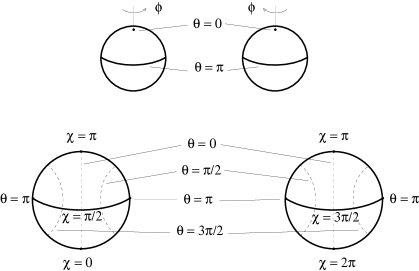
Figure 18: Top : Representation of ${\mathchoice{\hbox{\raise 3.41666pt\hbox to0.0pt{\kern 1.94447pt\vrule height=3.07497pt\hss}\hbox to0.0pt{\kern 3.05557pt\vrule height=3.41666pt\hss}\hbox{$\displaystyle\rm S$}}}{\hbox{\raise 3.41666pt\hbox to0.0pt{\kern 1.94447pt\vrule height=3.07497pt\hss}\hbox to0.0pt{\kern 3.05557pt\vrule height=3.41666pt\hss}\hbox{$\textstyle\rm S$}}}{\hbox{\raise 2.39166pt\hbox to0.0pt{\kern 1.36113pt\vrule height=2.15248pt\hss}\raise 0.23917pt\hbox to0.0pt{\kern 1.94444pt\vrule height=2.15248pt\hss}\hbox{$\scriptstyle\rm S$}}}{\hbox{\raise 1.70833pt\hbox to0.0pt{\kern 1.11108pt\vrule height=1.53748pt\hss}\raise 0.17084pt\hbox to0.0pt{\kern 1.52779pt\vrule height=1.53748pt\hss}\hbox{$\scriptscriptstyle\rm S$}}}}^{3}$ by two balls in ${\rm I\!R}^{3}$ glued together. Bottom : Behaviour of coordinates within slices $sin\phi=0$.

7.2 The holonomies of ${\mathchoice{\hbox{\raise 3.41666pt\hbox to0.0pt{\kern 1.94447pt\vrule height=3.07497pt\hss}\hbox to0.0pt{\kern 3.05557pt\vrule height=3.41666pt\hss}\hbox{$\displaystyle\rm S$}}}{\hbox{\raise 3.41666pt\hbox to0.0pt{\kern 1.94447pt\vrule height=3.07497pt\hss}\hbox to0.0pt{\kern 3.05557pt\vrule height=3.41666pt\hss}\hbox{$\textstyle\rm S$}}}{\hbox{\raise 2.39166pt\hbox to0.0pt{\kern 1.36113pt\vrule height=2.15248pt\hss}\raise 0.23917pt\hbox to0.0pt{\kern 1.94444pt\vrule height=2.15248pt\hss}\hbox{$\scriptstyle\rm S$}}}{\hbox{\raise 1.70833pt\hbox to0.0pt{\kern 1.11108pt\vrule height=1.53748pt\hss}\raise 0.17084pt\hbox to0.0pt{\kern 1.52779pt\vrule height=1.53748pt\hss}\hbox{$\scriptscriptstyle\rm S$}}}}^{3}$

The full isometry group of ${\mathchoice{\hbox{\raise 3.41666pt\hbox to0.0pt{\kern 1.94447pt\vrule height=3.07497pt\hss}\hbox to0.0pt{\kern 3.05557pt\vrule height=3.41666pt\hss}\hbox{$\displaystyle\rm S$}}}{\hbox{\raise 3.41666pt\hbox to0.0pt{\kern 1.94447pt\vrule height=3.07497pt\hss}\hbox to0.0pt{\kern 3.05557pt\vrule height=3.41666pt\hss}\hbox{$\textstyle\rm S$}}}{\hbox{\raise 2.39166pt\hbox to0.0pt{\kern 1.36113pt\vrule height=2.15248pt\hss}\raise 0.23917pt\hbox to0.0pt{\kern 1.94444pt\vrule height=2.15248pt\hss}\hbox{$\scriptstyle\rm S$}}}{\hbox{\raise 1.70833pt\hbox to0.0pt{\kern 1.11108pt\vrule height=1.53748pt\hss}\raise 0.17084pt\hbox to0.0pt{\kern 1.52779pt\vrule height=1.53748pt\hss}\hbox{$\scriptscriptstyle\rm S$}}}}^{3}$ is $SO(4)$. A modern summary by Wolf [158] gives an explicit description of each admissible subgroup $\Gamma$ of $SO(4)$ without fixed point, acting freely and discontinuosly on ${\mathchoice{\hbox{\raise 3.41666pt\hbox to0.0pt{\kern 1.94447pt\vrule height=3.07497pt\hss}\hbox to0.0pt{\kern 3.05557pt\vrule height=3.41666pt\hss}\hbox{$\displaystyle\rm S$}}}{\hbox{\raise 3.41666pt\hbox to0.0pt{\kern 1.94447pt\vrule height=3.07497pt\hss}\hbox to0.0pt{\kern 3.05557pt\vrule height=3.41666pt\hss}\hbox{$\textstyle\rm S$}}}{\hbox{\raise 2.39166pt\hbox to0.0pt{\kern 1.36113pt\vrule height=2.15248pt\hss}\raise 0.23917pt\hbox to0.0pt{\kern 1.94444pt\vrule height=2.15248pt\hss}\hbox{$\scriptstyle\rm S$}}}{\hbox{\raise 1.70833pt\hbox to0.0pt{\kern 1.11108pt\vrule height=1.53748pt\hss}\raise 0.17084pt\hbox to0.0pt{\kern 1.52779pt\vrule height=1.53748pt\hss}\hbox{$\scriptscriptstyle\rm S$}}}}^{3}$ :

• the cyclic group of order p, $Z_{p}$ ($p\geq 2$).

  A cyclic group just consists of the powers of a single element : $a,a^{2},\ldots,a^{p}=Id.$ (for instance the $p^{th}$ roots of unity $exp(2\pi~{}mi/p),~{}m=0,1,\ldots,p-1$). In a more geometrical representation, $Z_{p}$ can be seen as generated by the rotations by an angle $2\pi/p$ about an arbitrary axis [$\theta$,$\phi$] of ${\rm I\!R}^{3}$.

• the dihedral group of order $2m$, $D_{m}$ ($m>2$).

  $D_{m}$ is generated by two elements $A$ and $S$ such that (in matrix notation) $A^{m}=Id.$, $S^{2}=Id.$, $SAS^{-1}=cA^{-1}$, where $c=exp(2\pi~{}ki/m)$ is a $m^{th}$ root of unity. In a more geometrical representation, $D_{m}$ can be viewed as generated by the rotations in the plane by an angle $2\pi/m$ and a flip about a line through the origin. Such symmetries preserve a regular m-gon lying in the plane and centered on the origin (figure 19).

  

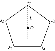
  Figure 19: The dihedral group $D_{5}$. The pentagon $J_{1}\ldots J_{5}$ is invariant by rotations of angle $2\pi/5$ about the line L.

• the polyhedral groups

  They are the symmetry groups of the regular polyhedra in ${\rm I\!R}^{3}$ (figure 20), namely :

  • the group $T$ of the tetrahedron (4 vertices, 6 edges, 4 faces), of order 12;

  • the group $O$ of the octahedron (6 vertices, 12 edges, 8 faces), of order 24 ;

  • the group $I$ of the isocahedron (12 vertices, 30 edges, 20 faces), of order 60.

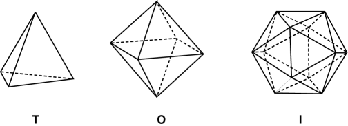
Figure 20: The polyhedral groups. Left: Tetrahedral group. Center: Octahedral group. Right: Icosahedral group.

Note that there are two other regular polyhedra (historically known as the Platonic solids) : the hexahedron (cube) and the dodecahedron (12 faces). But the cube has the same symmetry group as the octahedron, and the dodecahedron has the same symmetry group as the icosahedron.

All the homogeneous spaces of constant positive curvature are obtained by quotienting ${\mathchoice{\hbox{\raise 3.41666pt\hbox to0.0pt{\kern 1.94447pt\vrule height=3.07497pt\hss}\hbox to0.0pt{\kern 3.05557pt\vrule height=3.41666pt\hss}\hbox{$\displaystyle\rm S$}}}{\hbox{\raise 3.41666pt\hbox to0.0pt{\kern 1.94447pt\vrule height=3.07497pt\hss}\hbox to0.0pt{\kern 3.05557pt\vrule height=3.41666pt\hss}\hbox{$\textstyle\rm S$}}}{\hbox{\raise 2.39166pt\hbox to0.0pt{\kern 1.36113pt\vrule height=2.15248pt\hss}\raise 0.23917pt\hbox to0.0pt{\kern 1.94444pt\vrule height=2.15248pt\hss}\hbox{$\scriptstyle\rm S$}}}{\hbox{\raise 1.70833pt\hbox to0.0pt{\kern 1.11108pt\vrule height=1.53748pt\hss}\raise 0.17084pt\hbox to0.0pt{\kern 1.52779pt\vrule height=1.53748pt\hss}\hbox{$\scriptscriptstyle\rm S$}}}}^{3}$ with the groups described above. They are in infinite number due to parameters $p$ and $m$.

7.3 The size of spherical 3-spaces

The volume of $\cal M$$={\mathchoice{\hbox{\raise 3.41666pt\hbox to0.0pt{\kern 1.94447pt\vrule height=3.07497pt\hss}\hbox to0.0pt{\kern 3.05557pt\vrule height=3.41666pt\hss}\hbox{$\displaystyle\rm S$}}}{\hbox{\raise 3.41666pt\hbox to0.0pt{\kern 1.94447pt\vrule height=3.07497pt\hss}\hbox to0.0pt{\kern 3.05557pt\vrule height=3.41666pt\hss}\hbox{$\textstyle\rm S$}}}{\hbox{\raise 2.39166pt\hbox to0.0pt{\kern 1.36113pt\vrule height=2.15248pt\hss}\raise 0.23917pt\hbox to0.0pt{\kern 1.94444pt\vrule height=2.15248pt\hss}\hbox{$\scriptstyle\rm S$}}}{\hbox{\raise 1.70833pt\hbox to0.0pt{\kern 1.11108pt\vrule height=1.53748pt\hss}\raise 0.17084pt\hbox to0.0pt{\kern 1.52779pt\vrule height=1.53748pt\hss}\hbox{$\scriptscriptstyle\rm S$}}}}^{3}/\Gamma$ is simply

$$vol({\cal M})=2\pi^{2}~{}R^{3}/\mid\Gamma\mid$$ (29)

where $\mid\Gamma\mid$ is the order of the group $\Gamma$. For topologically complicated spherical 3–manifolds, $\mid\Gamma\mid$ becomes large and $vol(\cal{M})$ is small. There is no lower bound since $\Gamma$ can have an arbitrarily large number of elements. In contrast, the diameter, i.e., the maximum distance between two points in the space, is bounded below by $\frac{1}{2}arccos((1/\sqrt{3})~{}cotg\pi/5)~{}R\approx 0.326~{}R$, corresponding to a dodecahedral space [10].

7.4 Examples

7.4.1 The projective space

${\rm I\!P}^{3}={\mathchoice{\hbox{\raise 3.41666pt\hbox to0.0pt{\kern 1.94447pt\vrule height=3.07497pt\hss}\hbox to0.0pt{\kern 3.05557pt\vrule height=3.41666pt\hss}\hbox{$\displaystyle\rm S$}}}{\hbox{\raise 3.41666pt\hbox to0.0pt{\kern 1.94447pt\vrule height=3.07497pt\hss}\hbox to0.0pt{\kern 3.05557pt\vrule height=3.41666pt\hss}\hbox{$\textstyle\rm S$}}}{\hbox{\raise 2.39166pt\hbox to0.0pt{\kern 1.36113pt\vrule height=2.15248pt\hss}\raise 0.23917pt\hbox to0.0pt{\kern 1.94444pt\vrule height=2.15248pt\hss}\hbox{$\scriptstyle\rm S$}}}{\hbox{\raise 1.70833pt\hbox to0.0pt{\kern 1.11108pt\vrule height=1.53748pt\hss}\raise 0.17084pt\hbox to0.0pt{\kern 1.52779pt\vrule height=1.53748pt\hss}\hbox{$\scriptscriptstyle\rm S$}}}}^{3}/{\mathchoice{\hbox{$\sf\textstyle Z\kern-3.99994ptZ$}}{\hbox{$\sf\textstyle Z\kern-3.99994ptZ$}}{\hbox{$\sf\scriptstyle Z\kern-2.10002ptZ$}}{\hbox{$\sf\scriptscriptstyle Z\kern-0.99998ptZ$}}}_{2}$ is obtained by identifying on ${\mathchoice{\hbox{\raise 3.41666pt\hbox to0.0pt{\kern 1.94447pt\vrule height=3.07497pt\hss}\hbox to0.0pt{\kern 3.05557pt\vrule height=3.41666pt\hss}\hbox{$\displaystyle\rm S$}}}{\hbox{\raise 3.41666pt\hbox to0.0pt{\kern 1.94447pt\vrule height=3.07497pt\hss}\hbox to0.0pt{\kern 3.05557pt\vrule height=3.41666pt\hss}\hbox{$\textstyle\rm S$}}}{\hbox{\raise 2.39166pt\hbox to0.0pt{\kern 1.36113pt\vrule height=2.15248pt\hss}\raise 0.23917pt\hbox to0.0pt{\kern 1.94444pt\vrule height=2.15248pt\hss}\hbox{$\scriptstyle\rm S$}}}{\hbox{\raise 1.70833pt\hbox to0.0pt{\kern 1.11108pt\vrule height=1.53748pt\hss}\raise 0.17084pt\hbox to0.0pt{\kern 1.52779pt\vrule height=1.53748pt\hss}\hbox{$\scriptscriptstyle\rm S$}}}}^{3}$ diametrically opposite points :

$(x^{1},x^{2},x^{3},x^{4})\equiv(-x^{1},-x^{2},-x^{3},-x^{4})$ in (25), or, equivalently,

$(\chi,\theta,\phi)\equiv(\pi-\chi,\pi-\theta,\pi+\phi)$ in (26).

In contrast with its 2–dimensional analogue ${\rm I\!P}^{2}$, ${\rm I\!P}^{3}$ is orientable. Its volume is $\pi^{2}R^{3}$. In ${\mathchoice{\hbox{\raise 3.41666pt\hbox to0.0pt{\kern 1.94447pt\vrule height=3.07497pt\hss}\hbox to0.0pt{\kern 3.05557pt\vrule height=3.41666pt\hss}\hbox{$\displaystyle\rm S$}}}{\hbox{\raise 3.41666pt\hbox to0.0pt{\kern 1.94447pt\vrule height=3.07497pt\hss}\hbox to0.0pt{\kern 3.05557pt\vrule height=3.41666pt\hss}\hbox{$\textstyle\rm S$}}}{\hbox{\raise 2.39166pt\hbox to0.0pt{\kern 1.36113pt\vrule height=2.15248pt\hss}\raise 0.23917pt\hbox to0.0pt{\kern 1.94444pt\vrule height=2.15248pt\hss}\hbox{$\scriptstyle\rm S$}}}{\hbox{\raise 1.70833pt\hbox to0.0pt{\kern 1.11108pt\vrule height=1.53748pt\hss}\raise 0.17084pt\hbox to0.0pt{\kern 1.52779pt\vrule height=1.53748pt\hss}\hbox{$\scriptscriptstyle\rm S$}}}}^{3}$, any two geodesics starting from a point intersect also at the antipodal point, at a distance $\pi R$ measured along any of these lines. In ${\rm I\!P}^{3}$, two geodesics cannot have more than one point in common.

7.4.2 A lens space

The spaces ${\mathchoice{\hbox{\raise 3.41666pt\hbox to0.0pt{\kern 1.94447pt\vrule height=3.07497pt\hss}\hbox to0.0pt{\kern 3.05557pt\vrule height=3.41666pt\hss}\hbox{$\displaystyle\rm S$}}}{\hbox{\raise 3.41666pt\hbox to0.0pt{\kern 1.94447pt\vrule height=3.07497pt\hss}\hbox to0.0pt{\kern 3.05557pt\vrule height=3.41666pt\hss}\hbox{$\textstyle\rm S$}}}{\hbox{\raise 2.39166pt\hbox to0.0pt{\kern 1.36113pt\vrule height=2.15248pt\hss}\raise 0.23917pt\hbox to0.0pt{\kern 1.94444pt\vrule height=2.15248pt\hss}\hbox{$\scriptstyle\rm S$}}}{\hbox{\raise 1.70833pt\hbox to0.0pt{\kern 1.11108pt\vrule height=1.53748pt\hss}\raise 0.17084pt\hbox to0.0pt{\kern 1.52779pt\vrule height=1.53748pt\hss}\hbox{$\scriptscriptstyle\rm S$}}}}^{3}/{\mathchoice{\hbox{$\sf\textstyle Z\kern-3.99994ptZ$}}{\hbox{$\sf\textstyle Z\kern-3.99994ptZ$}}{\hbox{$\sf\scriptstyle Z\kern-2.10002ptZ$}}{\hbox{$\sf\scriptscriptstyle Z\kern-0.99998ptZ$}}}_{p}$ are called lens spaces, due to the shape of their fundamental domain. Apart from the projective space, the simplest lens space is ${\mathchoice{\hbox{\raise 3.41666pt\hbox to0.0pt{\kern 1.94447pt\vrule height=3.07497pt\hss}\hbox to0.0pt{\kern 3.05557pt\vrule height=3.41666pt\hss}\hbox{$\displaystyle\rm S$}}}{\hbox{\raise 3.41666pt\hbox to0.0pt{\kern 1.94447pt\vrule height=3.07497pt\hss}\hbox to0.0pt{\kern 3.05557pt\vrule height=3.41666pt\hss}\hbox{$\textstyle\rm S$}}}{\hbox{\raise 2.39166pt\hbox to0.0pt{\kern 1.36113pt\vrule height=2.15248pt\hss}\raise 0.23917pt\hbox to0.0pt{\kern 1.94444pt\vrule height=2.15248pt\hss}\hbox{$\scriptstyle\rm S$}}}{\hbox{\raise 1.70833pt\hbox to0.0pt{\kern 1.11108pt\vrule height=1.53748pt\hss}\raise 0.17084pt\hbox to0.0pt{\kern 1.52779pt\vrule height=1.53748pt\hss}\hbox{$\scriptscriptstyle\rm S$}}}}^{3}/{\mathchoice{\hbox{$\sf\textstyle Z\kern-3.99994ptZ$}}{\hbox{$\sf\textstyle Z\kern-3.99994ptZ$}}{\hbox{$\sf\scriptstyle Z\kern-2.10002ptZ$}}{\hbox{$\sf\scriptscriptstyle Z\kern-0.99998ptZ$}}}_{3}$, which divides ${\mathchoice{\hbox{\raise 3.41666pt\hbox to0.0pt{\kern 1.94447pt\vrule height=3.07497pt\hss}\hbox to0.0pt{\kern 3.05557pt\vrule height=3.41666pt\hss}\hbox{$\displaystyle\rm S$}}}{\hbox{\raise 3.41666pt\hbox to0.0pt{\kern 1.94447pt\vrule height=3.07497pt\hss}\hbox to0.0pt{\kern 3.05557pt\vrule height=3.41666pt\hss}\hbox{$\textstyle\rm S$}}}{\hbox{\raise 2.39166pt\hbox to0.0pt{\kern 1.36113pt\vrule height=2.15248pt\hss}\raise 0.23917pt\hbox to0.0pt{\kern 1.94444pt\vrule height=2.15248pt\hss}\hbox{$\scriptstyle\rm S$}}}{\hbox{\raise 1.70833pt\hbox to0.0pt{\kern 1.11108pt\vrule height=1.53748pt\hss}\raise 0.17084pt\hbox to0.0pt{\kern 1.52779pt\vrule height=1.53748pt\hss}\hbox{$\scriptscriptstyle\rm S$}}}}^{3}$ into 6 fundamental cells, each having a lens form. The one centered onto the observer at coordinates, say, ($\chi=0,~{}\theta=0,~{}\phi_{0}$) has for boundaries : the great circle ($\chi=\theta=\pi/2,~{}0\leq\phi\leq 2\pi$); the cone of geodesics with summit ($\chi=\pi/6,~{}\theta=0$) and base the previous great circle ; the symmetric cone with summit ($\chi=\pi/6,~{}\theta=\pi$) and the same base. When this fundamental cell is translated, the points on the circle ($\chi=\theta=\pi/2,~{}\phi$) are transformed to ($\chi=\theta=\pi/2,~{}\phi+\pi/3)$. Similarly the points on the circle $\theta=0$ have their value of $\chi$ increased by $\pi/3$. The maximum dimension of the fundamental lens is $\pi R/2$. The observer has 5 images of itself given by ($\pi/3,~{}0,~{}\phi_{0}$), ($2\pi/3,~{}0,~{}\phi_{0}$), ($\pi,~{}0,~{}\phi_{0}$), ($2\pi/3,~{}\pi,~{}\pi+\phi_{0}$), ($\pi/3,~{}\pi,~{}\pi+\phi_{0}$).

7.4.3 A dihedral space

The simplest “dihedral” space is ${\mathchoice{\hbox{\raise 3.41666pt\hbox to0.0pt{\kern 1.94447pt\vrule height=3.07497pt\hss}\hbox to0.0pt{\kern 3.05557pt\vrule height=3.41666pt\hss}\hbox{$\displaystyle\rm S$}}}{\hbox{\raise 3.41666pt\hbox to0.0pt{\kern 1.94447pt\vrule height=3.07497pt\hss}\hbox to0.0pt{\kern 3.05557pt\vrule height=3.41666pt\hss}\hbox{$\textstyle\rm S$}}}{\hbox{\raise 2.39166pt\hbox to0.0pt{\kern 1.36113pt\vrule height=2.15248pt\hss}\raise 0.23917pt\hbox to0.0pt{\kern 1.94444pt\vrule height=2.15248pt\hss}\hbox{$\scriptstyle\rm S$}}}{\hbox{\raise 1.70833pt\hbox to0.0pt{\kern 1.11108pt\vrule height=1.53748pt\hss}\raise 0.17084pt\hbox to0.0pt{\kern 1.52779pt\vrule height=1.53748pt\hss}\hbox{$\scriptscriptstyle\rm S$}}}}^{3}/D_{3}$. It divides the 3–sphere into 12 trihedral cells. The observer at coordinates $(0,0,0)$ has 11 images of himself at coordinates $(\pi/3,~{}0,~{}0)$, $(2\pi/3,~{}0,~{}0)$, $(\pi,~{}0,~{}0)$, $(2\pi/3,~{}\pi,~{}0)$, $(\pi/3,~{}\pi,~{}0)$, $(\pi/2,~{}\pi/2,~{}0)$, $(\pi/2,~{}\pi/2,~{}\pi/3)$, $(\pi/2,~{}\pi/2,~{}2\pi/3)$, $(\pi/2,~{}\pi/2,~{}\pi)$, $(\pi/2,~{}\pi/2,~{}4\pi/3)$, $(\pi/2,~{}\pi/2,~{}5\pi/3).$

7.4.4 The Poincaré dodecahedral space

The Poincaré manifold [127] is an example of ${\mathchoice{\hbox{\raise 3.41666pt\hbox to0.0pt{\kern 1.94447pt\vrule height=3.07497pt\hss}\hbox to0.0pt{\kern 3.05557pt\vrule height=3.41666pt\hss}\hbox{$\displaystyle\rm S$}}}{\hbox{\raise 3.41666pt\hbox to0.0pt{\kern 1.94447pt\vrule height=3.07497pt\hss}\hbox to0.0pt{\kern 3.05557pt\vrule height=3.41666pt\hss}\hbox{$\textstyle\rm S$}}}{\hbox{\raise 2.39166pt\hbox to0.0pt{\kern 1.36113pt\vrule height=2.15248pt\hss}\raise 0.23917pt\hbox to0.0pt{\kern 1.94444pt\vrule height=2.15248pt\hss}\hbox{$\scriptstyle\rm S$}}}{\hbox{\raise 1.70833pt\hbox to0.0pt{\kern 1.11108pt\vrule height=1.53748pt\hss}\raise 0.17084pt\hbox to0.0pt{\kern 1.52779pt\vrule height=1.53748pt\hss}\hbox{$\scriptscriptstyle\rm S$}}}}^{3}/I$. The fundamental polyhedron is a regular dodecahedron whose faces are pentagons. The compact space is obtained in identifying the opposite faces after rotating by $1/10^{th}$ turn in the clockwise direction around the axis orthogonal to the face (figure 21). This configuration involves 120 successive operations and gives already some idea of the extreme complication of such multi–connected topologies.

8 Three-dimensional hyperbolic space forms

8.1 The geometry of ${\rm I\!H}^{3}$

Locally hyperbolic manifolds are by far less well understood than the other homogeneous spaces. However, according to the pionneering work of Thurston [150], “almost” all 3–manifolds can be endowed with a hyperbolic structure. Here we present some elements of the theory; for a recent report, see [9].

It is not easy to have an intuitive representation of ${\rm I\!H}^{3}$ because it cannot be imbedded in ${\rm I\!R}^{4}$. Instead, it can be seen as an hypersurface of equation $-(x^{1})^{2}+(x^{2})^{2}+(x^{3})^{2}+(x^{4})^{2}=R^{2}$ in the Minkowski space of metric $ds^{2}=-(dx^{1})^{2}+(dx^{2})^{2}+(dx^{3})^{2}+(dx^{4})^{2}$. Hence the generators of the fundamental group $G$ of ${\rm I\!H}^{3}$ are equivalent to homogeneous Lorentz transformations [31].

If we introduce coordinates $(\chi,\theta,\phi)$ by

$$x^{1}=R~{}cosh\chi,~{}x^{2}=R~{}sinh\chi~{}cos\theta,~{}x^{3}=R~{}sinh\chi~{}sin\theta~{}cos\phi,~{}x^{4}=R~{}sinh\chi~{}sin\theta~{}sin\phi$$

with $0\leq\chi<\infty$, $0\leq\theta\leq\pi$, $0\leq\phi\leq 2\pi$, the induced metric on ${\rm I\!H}^{3}$ may be written as

$$d\sigma^{2}=R^{2}~{}\Bigl{\{}~{}d\chi^{2}+sinh^{2}\chi~{}(d\theta^{2}+sin^{2}\theta~{}d\phi^{2})\Bigr{\}}$$ (30)

The volume is infinite. The Robertson–Walker form of the metric – generally used in relativistic cosmology – is obtained from the coordinate change $r=sinh\chi$, which puts the metric into :

$$d\sigma^{2}=R^{2}\Bigl{\{}\frac{dr^{2}}{1+r^{2}}+r^{2}(d\theta^{2}+sin^{2}\theta d\phi^{2})\Bigr{\}}$$ (31)

Other forms of the metric are commonly used :

• In the upper-half space representation, ${\rm I\!H}^{3}$ is mapped onto ${\rm I\!R}^{3}_{+}=\{(x,y,z)\in{\rm I\!R}^{3}\mid z>0\}$ equipped with the metric

  $$d\sigma^{2}=\frac{dx^{2}+dy^{2}+dz^{2}}{z^{2}}.$$ (32)

  The lines and planes of ${\rm I\!H}^{3}$ become semi–circles and semi–spheres of ${\rm I\!R}^{3}_{+}$, which orthogonally intersect with the boundary.

• In the Poincaré representation, ${\rm I\!H}^{3}$ is mapped into the unit open ball $\{(x,y,z,\in{\rm I\!R}^{3}\mid x^{2}+y^{2}+z^{2}<1\}$. Hyperbolic lines and planes are semi-circles and semi-spheres which orthogonally intersect the boundary ${\mathchoice{\hbox{\raise 3.41666pt\hbox to0.0pt{\kern 1.94447pt\vrule height=3.07497pt\hss}\hbox to0.0pt{\kern 3.05557pt\vrule height=3.41666pt\hss}\hbox{$\displaystyle\rm S$}}}{\hbox{\raise 3.41666pt\hbox to0.0pt{\kern 1.94447pt\vrule height=3.07497pt\hss}\hbox to0.0pt{\kern 3.05557pt\vrule height=3.41666pt\hss}\hbox{$\textstyle\rm S$}}}{\hbox{\raise 2.39166pt\hbox to0.0pt{\kern 1.36113pt\vrule height=2.15248pt\hss}\raise 0.23917pt\hbox to0.0pt{\kern 1.94444pt\vrule height=2.15248pt\hss}\hbox{$\scriptstyle\rm S$}}}{\hbox{\raise 1.70833pt\hbox to0.0pt{\kern 1.11108pt\vrule height=1.53748pt\hss}\raise 0.17084pt\hbox to0.0pt{\kern 1.52779pt\vrule height=1.53748pt\hss}\hbox{$\scriptscriptstyle\rm S$}}}}^{2}$.

• In the Klein model, ${\rm I\!H}^{3}$ is mapped into the unit open ball in ${\rm I\!R}^{3}$, with Cartesian coordinates $(x^{i})$, with the correspondence :

  $$x^{1}=\tanh\chi~{}\sin\theta~{}\cos\phi,~{}x^{2}=\tanh\chi~{}\sin\theta~{}\sin\phi,~{}x^{3}=\tanh\chi~{}\cos\theta.$$ (33)

  Then the distance between 2 points ${\bf x}$ and ${\bf y}$ writes :

  $$d({\bf x},{\bf y})=cosh^{-1}~{}\Bigl{[}\frac{1-{\bf x}.{\bf y}}{(1-{\bf x}.{\bf x})~{}(1-{\bf y}.{\bf y})}\Bigr{]}^{1/2}.$$ (34)

  The advantage of such a representation is that hyperbolic lines and planes are mapped into their Euclidean counterparts.

8.2 The holonomies of ${\rm I\!H}^{3}$

The isometries of ${\rm I\!H}^{3}$ are most conveniently described in the upper–half space model ${\rm I\!R}^{3}_{+}$. Their group is isomorphic to $PSL(2,{\mathchoice{\hbox{\hbox to0.0pt{\kern 2.88884pt\vrule height=6.14993pt\hss}\hbox{$\displaystyle\rm C$}}}{\hbox{\hbox to0.0pt{\kern 2.88884pt\vrule height=6.14993pt\hss}\hbox{$\textstyle\rm C$}}}{\hbox{\hbox to0.0pt{\kern 2.02219pt\vrule height=4.30496pt\hss}\hbox{$\scriptstyle\rm C$}}}{\hbox{\hbox to0.0pt{\kern 1.44441pt\vrule height=3.07497pt\hss}\hbox{$\scriptscriptstyle\rm C$}}}})$, namely the group of fractional linear transformations acting on the complex  plane :

$$z^{\prime}={az+b\over cz+d},~{}a,b,c,d\in{\mathchoice{\hbox{\hbox to0.0pt{\kern 2.88884pt\vrule height=6.14993pt\hss}\hbox{$\displaystyle\rm C$}}}{\hbox{\hbox to0.0pt{\kern 2.88884pt\vrule height=6.14993pt\hss}\hbox{$\textstyle\rm C$}}}{\hbox{\hbox to0.0pt{\kern 2.02219pt\vrule height=4.30496pt\hss}\hbox{$\scriptstyle\rm C$}}}{\hbox{\hbox to0.0pt{\kern 1.44441pt\vrule height=3.07497pt\hss}\hbox{$\scriptscriptstyle\rm C$}}}},~{}ad-bc=1.$$

This group operates also as the group of conformal transformations of ${\rm I\!R}^{3}$ which leaves the upper half space invariant. Finite subgroups are discussed in Beardon [7].

8.3 The size of compact hyperbolic manifolds

In hyperbolic geometry there is an essential difference between the 2–dimensional case and higher dimensions. A surface of genus $g\geq 2$ supports uncountably many non equivalent hyperbolic metrics. But for $n\geq 3$, a connected oriented n-smanifold supports at most one hyperbolic metric. More precisely, the rigidity theorem proves that if two hyperbolic manifolds, with dimension $n\geq 3$, have isomorphic fundamental groups, they are necessarily isometric to each other. This was proved by Mostow [113] in the compact case, and by Prasad [128] in the non–compact case. It follows that, for $n\geq 3$, the volume of a manifold and the lengths of its closed geodesics are topological invariants. This suggested the idea of using the volumes to classify the topologies, which could have seemed, at a first glance, contradictory with the very purpose of topology.

Each type of topology is characterized by some lengthes. For compact locally Euclidean spaces, the fundamental polyhedron may possess arbitrary volume, but no more than eight faces. In the spherical case, the volume of ${\mathchoice{\hbox{\raise 3.41666pt\hbox to0.0pt{\kern 1.94447pt\vrule height=3.07497pt\hss}\hbox to0.0pt{\kern 3.05557pt\vrule height=3.41666pt\hss}\hbox{$\displaystyle\rm S$}}}{\hbox{\raise 3.41666pt\hbox to0.0pt{\kern 1.94447pt\vrule height=3.07497pt\hss}\hbox to0.0pt{\kern 3.05557pt\vrule height=3.41666pt\hss}\hbox{$\textstyle\rm S$}}}{\hbox{\raise 2.39166pt\hbox to0.0pt{\kern 1.36113pt\vrule height=2.15248pt\hss}\raise 0.23917pt\hbox to0.0pt{\kern 1.94444pt\vrule height=2.15248pt\hss}\hbox{$\scriptstyle\rm S$}}}{\hbox{\raise 1.70833pt\hbox to0.0pt{\kern 1.11108pt\vrule height=1.53748pt\hss}\raise 0.17084pt\hbox to0.0pt{\kern 1.52779pt\vrule height=1.53748pt\hss}\hbox{$\scriptscriptstyle\rm S$}}}}^{3}/\Gamma$ is finite and is an entire fraction of that of ${\mathchoice{\hbox{\raise 3.41666pt\hbox to0.0pt{\kern 1.94447pt\vrule height=3.07497pt\hss}\hbox to0.0pt{\kern 3.05557pt\vrule height=3.41666pt\hss}\hbox{$\displaystyle\rm S$}}}{\hbox{\raise 3.41666pt\hbox to0.0pt{\kern 1.94447pt\vrule height=3.07497pt\hss}\hbox to0.0pt{\kern 3.05557pt\vrule height=3.41666pt\hss}\hbox{$\textstyle\rm S$}}}{\hbox{\raise 2.39166pt\hbox to0.0pt{\kern 1.36113pt\vrule height=2.15248pt\hss}\raise 0.23917pt\hbox to0.0pt{\kern 1.94444pt\vrule height=2.15248pt\hss}\hbox{$\scriptstyle\rm S$}}}{\hbox{\raise 1.70833pt\hbox to0.0pt{\kern 1.11108pt\vrule height=1.53748pt\hss}\raise 0.17084pt\hbox to0.0pt{\kern 1.52779pt\vrule height=1.53748pt\hss}\hbox{$\scriptscriptstyle\rm S$}}}}^{3}$ (see eq. (29)), the maximum possible value. By contrast, it is possible to tesselate ${\rm I\!H}^{3}$ with polyhedra having an arbitrarily large number of faces. This was already the case in dimension two, with for instance the 4g-gones whose angles are thinned down by adjusting the surface on the hyperbolic plane. The role of the volume in ${\rm I\!H}^{3}$ generalizes that of the area in ${\rm I\!H}^{2}$. Correspondingly, in the three-dimensional hyperbolic case, the possible values for the volume of the $FP$ are bounded from below. In other words, there exists a hyperbolic 3–manifold with minimal volume.

Particular interest has been taken by various authors in computing the volumes of compact hyperbolic manifolds [117, 63, 92]. Little is known however about the set of all possible values of these volumes : the minimal one $vol_{min}$ is not known, nor whether any one is an irrational number  [150]. Thurston [151] proposed as a candidate for the hyperbolic 3–manifold of minimum volume a space $\cal Q$₁ with volume $vol({\cal Q}_{1})=0.98139~{}R^{3}$ (where $R$ is the curvature radius of the universal covering space). The conjecture turned out to be false when Weeks [154] and, independently, Matveev and Fomenko [107] found a compact hyperbolic $\cal Q$₂ such that $vol({\cal Q}_{2})=0.94272~{}R^{3}$. Since a ball of radius $R\chi$ has a volume $\pi R^{3}[sinh(2\chi)-2\chi]$, this corresponds to a diameter $\approx 0.6~{}R$.

However it is anyone’s guess how the real minimal value may be. Meyerhoff [109] has proved that $vol_{min}>0.00082R^{3}$. The smallest $vol_{min}$, the more interesting the corresponding manifold for cosmology (see next sections).

8.4 Examples

Topologists have been able to sketch a classification of compact hyperbolic spaces in terms of volumes. A topology is completely characterized by the number of faces of the fundamental polyhedron and by the various ways to identify them. This guarantees that the number of topological classes, although infinite, is countable.

The full classification of three–dimensional hyperbolic manifolds is far from being fully understood today, although it seems less unreachable than before. Various means are available to build an infinite number of hyperbolic spaces. Thurston [150] has given a procedure for effectively constructing hyperbolic structures by gluing together ideal polyhedra. The idea goes back to Poincaré, see e.g. [105]. However the construction of closed manifolds is far more complicated than that of non–compact ones [79, 1]. Many authors use the Dehn’s Surgery method, which consists in removing certain “regular” pieces of a manifold and gluing them back with a specific twist. We give below some well-known examples.

8.4.1 Non-compact models

• It is possible to construct a 3–space of constant negative curvature having the metric

  $$d\sigma^{2}=d\chi^{2}+\cosh^{2}\chi~{}d{\sigma^{\prime}}^{2},$$ (35)

  where $d{\sigma^{\prime}}^{2}$ is the metric (13) of a locally hyperbolic surface ${\rm I\!H}^{2}/\Gamma$. Since there is an infinite number of topologies on ${\rm I\!H}^{2}/\Gamma$, this offers a way of building an infinite number of topologies for locally hyperbolic spaces. These space are not compact in the direction orthogonal to ${\rm I\!H}^{2}/\Gamma$ ($-\infty<\chi<\infty$).

• Sokoloff and Starobinskii [143] have considered multi–connected hyperbolic spaces whose fundamental polyhedron is the non compact domain comprised between two “parallel” (that is, non intersecting) planes. With the coordinate transformation

  $$x=-\ln[\cosh\chi-\sinh\chi~{}\cos\theta]$$

  $$y=\frac{\sin\theta~{}\cos\phi}{\mbox{Argth}\chi-\cos\theta}$$

  $$z=\frac{\sin\theta~{}\sin\phi}{\mbox{Argth}\chi-\cos\theta}$$

  the metric (30) takes the form :

  $$d\sigma^{2}=dx^{2}+e^{-2x}(dy^{2}+dz^{2}).$$ (36)

  The boundaries of the fundamental domains are defined by the relation $a~{}e^{-x}=\Lambda$. Each domain (in particular the FP) represents the interior of a “cylindrical horn”. Holonomies occur via the identifications $y\rightarrow y+ma$, where $a$ is the circonference of the cylinder and $m$ an integer.

8.4.2 Compact models

The Seifert-Weber Space.

Seifert and Weber [138] have obtained a compact hyperbolic manifold whose fundamental polyhedron is a dodecahedron, with opposite pentagonal faces fitted together after twisting by 108 degrees (figure 21).

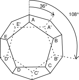
Figure 21: The spherical Poincaré space and the closed hyperbolic Seifert-Weber space are respectively obtained by identifying opposite faces of a regular dodecahedron after rotation by $\pi/5$ and $3\pi/5$.

The Löbell Space.

Löbell [98] has constructed a compact hyperbolic manifold, later on studied by Gott [72] in a cosmological context. The FP is a 14 faces polyhedron, two faces of which are regular rectangular hexagones and the 12 others rectangular regular pentagones (figure 22). The formulae of hyperbolic trigonometry permit to estimate the surfaces of the faces from their angular deficits : the area of each pentagon is $(\pi/2)R^{2}$, that of each hexagon is $\pi R^{2}$, while the edges have a length $1.32~{}R$. Around each vertex, 8 polyhedra can be placed and glued together to tesselate ${\rm I\!H}^{3}$. In fact, an infinite number of compact hyperbolic 3-spaces can be build by pasting together various numbers of these 14–hedra, and suitably identifying the unattached faces.

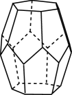
Figure 22: The FP for the Löbell topology is made of 8 such 14–hedra pasted together. All the angles in the figure are right angles in ${\rm I\!H}^{3}$.

The Best Spaces.

Best [11] has constructed several compact hyperbolic manifolds whose FP is a regular icosahedron. One of them was studied in details by Fagundes [48, 49] in a cosmological context. Its outer structure is represented in figure (23). The corresponding generators of the holonomy group are expressible in terms of $4\times 4$ matrices corresponding to homogeneous Lorentz transformations; for details, see Appendix A of [49]. The manifold is avantageously described in the Klein coordinates (33).

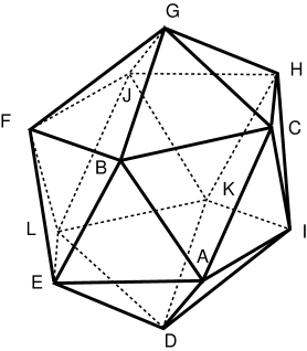
Figure 23: The closed hyperbolic Best space. The pairwise identifications of faces are $ADI\leftrightarrow BGC$, $ICA\leftrightarrow ABC$, $EFL\leftrightarrow DIK$, $DEL\leftrightarrow KLD$, $GFB\leftrightarrow HJK$, $FGJ\leftrightarrow GJH$, $ABE\leftrightarrow LJF$, $FEB\leftrightarrow CGH$, $AED\leftrightarrow KIH$, $JKL\leftrightarrow CHI$ (where the order of vertices in the faces in maintained in the identification).

The Weeks Space

The Weeks manifold [154] is a polyhedron with 26 vertices and 18 faces, among which 12 are pentagons and 6 are tetragons. Its outer structure is represented in figure (24). It has the peculiarity to be the smallest compact hyperbolic manifold presently known. Given the fact that, in quantum cosmology, the probability for spontaneous creation of a compact universe is bigger for a small one than for a large one, the Weeks space was studied by Fagundes [51] in a cosmological context. Fagundes provides also numerically the coordinates of the vertices and the 18 generators of the holonomy group (also expressible in terms of $4\times 4$ matrices corresponding to Lorentz transformations).

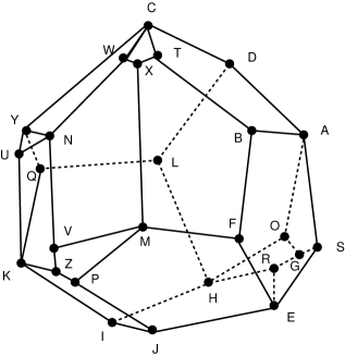
Figure 24: The closed hyperbolic Weeks space. The pairwise identifications of faces are $ABTCD\leftrightarrow HLDAO$, $SEFBA\leftrightarrow FMPJE$, $RHIJE\leftrightarrow IKQLH$, $FMXTB\leftrightarrow UKZVN$, $WNUYC\leftrightarrow IJPZK$, $CYQLD\leftrightarrow MXWNV$, $CTXW\leftrightarrow HOGR$, $KQYU\leftrightarrow ERGS$, $MPZV\leftrightarrow ASGO$.

9 Multi–connected cosmological models

9.1 Simply and multi–connected models

The metric of spacetime specifies its local geometry but not its topology. Such a metric, solution of the Einstein’s equations for a given form of the cosmic stress–energy tensor, may correspond to different models of the Universe with different spatial topologies. On the other hand, the local property of being a solution of the Einstein’s equations does not automatically guarantee that the boundary conditions are satisfied. Thus, solutions corresponding to the same metric but to distinct topologies may have different status.

Among the cosmological models, the most usually considered in the litterature are those with simply–connected space. We will refer generically to them as the Simply–Connected Models, hereafter SCM’s. However, the assumption of simple–connectedness is arbitrary and can be dropped out. Our interest in this paper focusses on the multi–connected cosmological models (hereafter MCM’s), defined as those having multi–connected (oriented) spatial sections . All of them obey the Einstein’s equations.

The most celebrated cosmological solutions of Einstein’s equations are the homogeneous and isotropic Friedmann–Lemaître  (FL) models, which obey the cosmological principe, i.e., where spatial sections have constant curvature. Beside the usual “big–bang” solutions, the FL models also include the de Sitter solution, as well as those incorporating a cosmological constant, or a non standard equation of state. From a spatial point of view, the FL models fall into 3 general classes, according to the sign of their spatial curvature $k=-1$, 0, or $+1$. The spacetime manifold is advantageously described by the Robertson–Walker metric

$$ds^{2}=c^{2}~{}dt^{2}-R^{2}(t)~{}d\sigma^{2},$$ (37)

where

$$d\sigma^{2}=d\chi^{2}+S_{k}^{2}(\chi)(d\theta^{2}+sin^{2}\theta~{}d\phi^{2})$$

is the metric of a 3–dimensional homogeneous manifold, flat ($k=0$, see eq. 24) or with curvature ($k=\pm 1$, see eq. 28, 30). We have defined the function

$$\left\{\begin{array}[]{ll}S_{k}(\chi)=\sinh(\chi)&\mbox{if $k=-1$}\\ S_{k}(\chi)=\chi&\mbox{if $k=0$}\\ S_{k}(\chi)=\sin(\chi)&\mbox{if $k=1$}\end{array}\right.$$

and $R(t)$ is the scale factor, chosen equal to the spatial curvature radius for non flat models, so that $k/R^{2}$ is the spatial curvature. The quadratic form $R^{2}(t)d\sigma^{2}$ denotes the metric of space at the cosmic time $t$, which remains homothetic during the cosmic evolution. The coordinates $\chi$, $\theta$ and $\phi$ are comoving : they remain the same for a cosmic object (a galaxy) in free fall, i.e., which follows the cosmic expansion. The proper distance (from the observer) to any object, evaluated at the present time $t_{0}$, is simply $d_{proper}=\chi~{}R(t_{0})$. It remains constant if the object exactly follows the expansion law and is called the proper comoving distance. The metric of the comoving space is $R_{0}^{2}~{}d\sigma^{2}$, $R_{0}=R(t_{0})$ being the present value of the scale factor.

Quite usually an other radial coordinate, the “circumference” coordinate $r=S_{k}(\chi)$, is used instead of $\chi$ in the metric. For simply–connected models, the whole space is described when the longitude (or right ascension) $\phi$ varies from $0$ to $2\pi$; the latitude (or declination) $\theta$ varies from $-\pi/2$ to $\pi/2$ ; the radial coordinate $\chi$ goes from $0$ to $\infty$ if $k=0$ or $-1$, or from $0$ to $\pi$ if $k=1$. If $r$ is used instead of $\chi$, it goes from $0$ to $\infty$ if $k=0$ or $-1$, or from 0 to 1, and then back from 1 to 0 if $k=1$. For multi–connected models, the space is smaller and the variation range of the coordinates $(\chi,\theta,\phi)$ is reduced.

To any MCM is associated an unique SCM sharing exactly the same kinematics and dynamics. The universal covering of the spatial sections of a MCM may be identified to the spatial sections of the corresponding SCM (${\rm I\!R}^{3}$, ${\rm I\!H}^{3}$ or ${\mathchoice{\hbox{\raise 3.41666pt\hbox to0.0pt{\kern 1.94447pt\vrule height=3.07497pt\hss}\hbox to0.0pt{\kern 3.05557pt\vrule height=3.41666pt\hss}\hbox{$\displaystyle\rm S$}}}{\hbox{\raise 3.41666pt\hbox to0.0pt{\kern 1.94447pt\vrule height=3.07497pt\hss}\hbox to0.0pt{\kern 3.05557pt\vrule height=3.41666pt\hss}\hbox{$\textstyle\rm S$}}}{\hbox{\raise 2.39166pt\hbox to0.0pt{\kern 1.36113pt\vrule height=2.15248pt\hss}\raise 0.23917pt\hbox to0.0pt{\kern 1.94444pt\vrule height=2.15248pt\hss}\hbox{$\scriptstyle\rm S$}}}{\hbox{\raise 1.70833pt\hbox to0.0pt{\kern 1.11108pt\vrule height=1.53748pt\hss}\raise 0.17084pt\hbox to0.0pt{\kern 1.52779pt\vrule height=1.53748pt\hss}\hbox{$\scriptscriptstyle\rm S$}}}}^{3}$ for FL models ) at the same time of its evolution. In particular, the scale factors $R(t)$ are exactly identical. In fact, most characteristics of the Friedmann–Lemaître models are preserved when we turn to the MCM’s, and this is a precious guide for their study.

It is presently believed that our Universe is correctly described by a Friedmann–Lemaître model. But the values of the cosmic parameters are not known accurately enough to decide the sign of the curvature. It is worth to remark that the multi–connectedness of space would provide an independant information on the cosmic parameters. For instance, the type of non–trivial topology observed would dictate the sign of the spatial curvature, since the structures of the holonomy groups are completely different for the cases $k=1,~{}0,~{}-1$. Thus, beside its own specific interest, multi–connectedness would offer a very efficient tool of investigation in observational cosmology.

9.2 Properties of the Friedmann–Lemaître models

The FL models are specified by the sign of the curvature ($k=0,-1$ or 1) and the scale factor $R(t)$, as it appears in the metric (37). As usual, we define the Hubble constant $H_{0}=\frac{\dot{R}}{R}\mid_{0}$, and the deceleration parameter $q_{0}=\frac{R\ddot{R}}{\dot{R}^{2}}\mid_{0}$, where the subscript $0$ means that the quantity is evaluated at the present time. Thus $H_{0}$ is also the constant appearing in the Hubble law $c~{}z=H_{0}~{}D$ for galaxies. The dynamics of the Universe, for the matter–dominated era,, i.e., in the last ten billion years, obeys the Friedmann equations in the following form :

$$\frac{\ddot{x}}{H_{0}^{2}}=\frac{\Omega}{2x^{2}}+\lambda~{}x$$ (38)

and

$$\frac{\dot{x}^{2}}{H_{0}^{2}}=\frac{\Omega}{x}+\lambda~{}x^{2}+1-\Omega-\lambda,$$ (39)

where

$$x(t)\equiv\frac{1}{1+z}=R(t)/R_{0}$$ (40)

and the dot denotes time differentiation. Note that, in this latter equation, the redshift $z=z(t)$ is regarded as a timelike coordinate, as usual in the Friedmann–Lemaître models. This is not contradictory with the use of $z$ as a spatial coordinate also, through the fact that the null geodesics establish a relation between look–back time and distance from the observer. As usual, $\Omega=8\pi~{}G\rho_{0}/3~{}H_{0}^{2}$ is the (present) density parameter of the universe and $\lambda=\Lambda/3~{}H_{0}^{2}$ is the “reduced” cosmological constant. These equations allow us to evaluate the function $R(t)$, to estimate the age of the universe (since the duration of the radiation era was negligible compared to that of the matter era), etc. We will often refer to $h$ as the Hubble constant $H_{0}$ in units of 100 km s^-1 Mpc^-1, so that distances estimated from redshifts are expressed in units of $h^{-1}~{}\mbox{Mpc}$. This defines the Hubble time $H_{0}^{-1}=9.78~{}10^{9}~{}h^{-1}$ years, and the Hubble length $c~{}H_{0}^{-1}=3000~{}h^{-1}~{}\mbox{Mpc}$. Note that the function $R(t)$ defines a correspondence between redshift and cosmic time through the relation (40) which holds in MCM’s as well as in SCM’s.

9.3 Homogeneity, Isotropy and Finiteness

The most commonly studied universe models are based onto the cosmological principle which implies spatial homogeneity. Also, spatial isotropy is assumed, in accordance with the observed distribution of cosmic objects, and with observations of the CMB. This implies, from Schur’s theorem, that space has constant curvature. The existing litterature on multi–connected cosmological models (with some exceptions, e.g.  [143, 45]) almost exclusively consider this case.

The isometry group $G/\Gamma$ of a manifold is smaller than $G$, that of its universal covering. As a consequence, the isotropy of space is broken in multi–connected models, excepted for the projective space (see §5.2). This breaking of symmetry may be apparent through the presence of some principal directions. In a cylinder ${\rm I\!R}\times S^{2}$ for instance, compact in 2 dimensions and infinite in the other, the metric tensor is exactly the same at every point : it keeps local homogeneity. However, it is not globally isotropic and has not the maximal symmetry. It is worthy to note that globally anisotropic models do not contradict observations, since the homogeneity of space and the local isotropy ensure the complete isotropy of the Cosmic Microwave Background, and the statistical isotropy of the distribution of discrete sources [35, 142, 43]. However, as we shall see in §12, global anisotropy can influence the spectrum of density fluctuations.

A major interest of the MCM’s come from the fact that the compact (finite) or non compact character of space is not linked to the sign of the curvature, unlike for the simply–connected ones. Multi–connected models with zero or negative curvature can be compact in some, or all their dimensions. For instance a toroidal universe, despite its zero spatial curvature, has a finite circumference and a finite volume which may in principle be measured. It contains a finite amount of matter. But a cylindrical universe (in the sense that the spatial sections are cylinders) is compact in 1 dimension only and has an infinite volume, although a finite circumference in the principal direction.

It is well known that, in the simply–connected big–bang  models, the homogeneity of space cannot be explained but is assumed in initial conditions. These initial conditions are often said, in this regard, to be very “special”, in the sense that curvature and all physical properties are identical in regions of space which have never been in causal contact : the values of the metric at different positions in space, although they may be seen as independent initial conditions, are indistinguishable, thus requiring a “fine tuning”. This so–called “homogeneity problem” has been particularly emphasized in relation with the Cosmic Microwave Background observations, which confirm the fundamental prediction of the big–bang models that the Universe was homogeneous better than to $10^{-5}$ at the recombination period, when this radiation was scattered for the last time.

It has been suggested that a past inflationary era could be an explanation for the homogeneity of the Universe. But convincing arguments in favor of inflation only exist in models where space was already homogeneous before inflation [69], so that the homogeneity problem is only pushed back in time. Moreover, no satisfactory model for inflation exists. In any case, there is no guarantee that inflation, which involves quantum effects interacting with gravity, may be treated in classical (i.e., non quantum) cosmology. No theory for quantum gravity or quantum cosmology is presently available. But it is certain that, if this happens, topological questions will have a very important role to play (see §9.4.1).

In order to explain the observed homogeneity of space, it would be tempting to invoke a causal process making homogeneous an initially heterogeneous universe. But, because of the causality constraints, such a process had no time to act before recombination, at a scale sufficiently large to account for the isotropy of the Cosmic Microwave Background. This is true in models without inflation. In models with inflation, on the other hand, causal processes had no time to homogeneize the universe before the occurrence of inflation, in order to allow this latter to start. Thus the past attempts to propose chaotic models which homogeneize with time [131] failed because of the observed isotropy of the Cosmic Microwave Background. Such models could however be reconciled with observations if the Universe is multi–connected [35, 36, 72]. In that case a small Universe could have become totally causally connected before the recombination period. We discuss this possibility in §12.1.

9.4 Quantum cosmology and the early Universe

9.4.1 Quantum cosmology

Since the general relativity  theory provides no prescription concerning the spatial topology, the questions of connectedness and homogeneity of the Universe may well finally relate to quantum cosmology. In classical (non quantum) relativity, a theorem due to Geroch [65] states that no topological change may occur in a non singular spacetime. However it is believed [67, 87] that a theory of quantum gravity, if any, would allow changes of the topology of space. Although this field is presently not fully developed, various approaches have been proposed to address the question of a quantum origin of the universe, or of quantum transitions in its very primordial state. Such studies are aimed to answer the questions concerning the origin of the geometry of the universe, the value of the cosmological constant, the material content, and the origin of cosmic fluctuations. In these approaches the connectedness of space plays a very important role since it is related to its compactness.

Here we do not intend to fully review these approaches but only briefly mention the role that topology can play. This problem has been addressed by various authors, (e.g. , [6, 70, 78]). Gurzadyan & Kocharyan [78] considered for instance the framework developed by Hawking & Hartle [80, 81]. Very shortly, a wave–function of the universe $\Psi$ is defined, which obeys the Wheeler–de Witt equation, an analog of the Schrödinger equation for quantum cosmology. $\mid\Psi\mid^{2}$ defines the amplitude of probability associated to the corresponding universe.

The wave–function $\Psi$ only depends on the characteristics of space and of its content, (but [78] consider only the case without matter, although with a cosmological constant), i.e., a 3–manifold $S$ with Riemaniann metric $h_{ij}$ and matter field configuration $\Phi$ on $S$. According to the “quantum–geometrodynamical” formalism, the wave function $\Psi$ may be calculated, in the quasi–classical approximation, as an integral over all 4–dimensional manifolds ${\cal M}$ which admit $S$ (with its metric) as a boundary. This defines the field of action for the Wheeler–de Witt equation : the infinite–dimensional space of all 3–dimensional Riemaniann metrics $h_{ij}$, called the superspace. Usually only homogeneous and isotropic closed spaces are considered, so that superspace is reduced to “minisuperspace”. In this framework, [78] have compared the probabilities for creation of universe with closed space, of constant positive (${\mathchoice{\hbox{\raise 3.41666pt\hbox to0.0pt{\kern 1.94447pt\vrule height=3.07497pt\hss}\hbox to0.0pt{\kern 3.05557pt\vrule height=3.41666pt\hss}\hbox{$\displaystyle\rm S$}}}{\hbox{\raise 3.41666pt\hbox to0.0pt{\kern 1.94447pt\vrule height=3.07497pt\hss}\hbox to0.0pt{\kern 3.05557pt\vrule height=3.41666pt\hss}\hbox{$\textstyle\rm S$}}}{\hbox{\raise 2.39166pt\hbox to0.0pt{\kern 1.36113pt\vrule height=2.15248pt\hss}\raise 0.23917pt\hbox to0.0pt{\kern 1.94444pt\vrule height=2.15248pt\hss}\hbox{$\scriptstyle\rm S$}}}{\hbox{\raise 1.70833pt\hbox to0.0pt{\kern 1.11108pt\vrule height=1.53748pt\hss}\raise 0.17084pt\hbox to0.0pt{\kern 1.52779pt\vrule height=1.53748pt\hss}\hbox{$\scriptscriptstyle\rm S$}}}}^{3}$ or a multi–connected space having ${\mathchoice{\hbox{\raise 3.41666pt\hbox to0.0pt{\kern 1.94447pt\vrule height=3.07497pt\hss}\hbox to0.0pt{\kern 3.05557pt\vrule height=3.41666pt\hss}\hbox{$\displaystyle\rm S$}}}{\hbox{\raise 3.41666pt\hbox to0.0pt{\kern 1.94447pt\vrule height=3.07497pt\hss}\hbox to0.0pt{\kern 3.05557pt\vrule height=3.41666pt\hss}\hbox{$\textstyle\rm S$}}}{\hbox{\raise 2.39166pt\hbox to0.0pt{\kern 1.36113pt\vrule height=2.15248pt\hss}\raise 0.23917pt\hbox to0.0pt{\kern 1.94444pt\vrule height=2.15248pt\hss}\hbox{$\scriptstyle\rm S$}}}{\hbox{\raise 1.70833pt\hbox to0.0pt{\kern 1.11108pt\vrule height=1.53748pt\hss}\raise 0.17084pt\hbox to0.0pt{\kern 1.52779pt\vrule height=1.53748pt\hss}\hbox{$\scriptscriptstyle\rm S$}}}}^{3}$ as universal covering), zero ($T^{3}$ or a multi–connected closed space having ${\rm I\!R}^{3}$ as universal covering), or negative (a multi–connected space having ${\rm I\!H}^{3}$ as universal covering) curvature. They conclude that the creation probability of a spherical Friedmann–Lemaître universe is larger than a toroidal one, which is itself larger than one with negative curvature. For inflationary universe (defined as created with a very high Hubble parameter), the 3 probabilities become equal. They also calculated the probability that a transition with a change in the topology of the universe, allowed in quantum (although not in classical) cosmology, occurs. For a toy–model, they found that the transition from a sphere to a torus (with equal volumes) is practically impossible, for instance much less probable than a transition from a sphere to an other one with different radius.

We do not want to insist too much on the details of these results, in which matter and matter creation have been neglected. Moreover, quantum cosmology is only very tentative and lacks an admitted interpretation. But we want to emphasize that :

- Connectedness is to play in quantum cosmology a role as much important, and probably more, than curvature.

- Multi–connected models are at least as probable than simply–connected ones.

9.4.2 Quantum effects in the early universe

By the play of expansion, the spatial dimensions of a MCM were very small in the primordial universe. In the first moments they may have been comparable to the scales of microphysics and quantum physics, thus allowing quantum and other peculiar effects. This is related to the thermal story of the primordial Universe, the generation of primordial fluctuations, the matter–antimatter asymmetry, etc.

Quantum field theory plays an important role in the description of the early universe : the distributions and properties of the matter, radiation, and energy contents rely on quantum physics and statistics. It has also been realized in the recent years that quantum physics could also play a role through the fundamental state – the vacuum – of some quantum fields. The popular inflation idea, for instance, results from the hypothesis that the dynamics of the Universe was dominated by the vacuum energy in a distant past, also in relation with the question of the cosmological constant.

There is no wide consensus over the concept of vacuum energy which lies at the interface between quantum physics and general relativity, not compatible in this regard. On the other hand, the Casimir effect [20], observed in the laboratory, has been interpreted in terms of vacuum energy, i.e., the energy of a fundamental state of a quantum field. Quantization in flat space is usually made with boundary conditions at infinity. Some constraints (like the interposition of conducting plates for an electromagnetic field) may impose different boundary conditions at finite distance. The consequence is the suppression of some modes for the vacuum state, with a different associated energy. The observed Casimir effect is interpreted as the (dynamical) consequence of the energy difference between the 2 different vacuum energies, with and without the plates.

This has led to the idea that vacuum energy, and vacuum energy differences can play a role in cosmology. We must however recall that the concept of an absolute vacuum energy remains controversial. Even the interpretation of the vacuum energy differences associated to the Casimir effect are not very clear. Despite these difficulties, such considerations have been extended to curved spacetime. This is the case of the Unruh (quantum vacuum effect in Rindler space, i.e., in the space seen by an accelerated observer) and Hawking (quantum effect in the vicinity of a black hole) effects, which present analogies with the Casimir effect. But there is no consensus either about the generalization of quantum theory, not speaking about vacuum effects, to curved spacetime. All these effects are induced by a modification of the boundary conditions imposed to quantum fields. Since the multi–connectedness of space would also modify those (by closing space), similar consequences may be expected.

Bytsenko & Goncharov ([19, 71]) have evaluated the topogical Casimir effect of a massless real scalar field on multi–connected spacetimes. Already for a fixed spacetime model, with a given topology (characterized by its holonomy group $\Gamma$), they remarked that different topologically inequivalent configurations of the scalar field do exist. To each such configuration $C$ is associated a different vacuum energy, called “Casimir energy” $E$. It is defined, as usual in quantum field theory, as the vacuum expectation value of the corresponding hamiltonian $H$

$$E(\Gamma,C)=<0\mid H\mid 0>,$$

which depends both on $\Gamma$ and $C$. Considering hyperbolic spacetimes ${\rm I\!R}\times{\rm I\!H}^{n}/\Gamma$, of dimension $n+1$, where ${\rm I\!R}$ is the time line, ${\rm I\!H}^{n}$ is the $n$–dimensional Lobachevsky space and $\Gamma$ a discrete group of isometries of ${\rm I\!H}^{n}$ without fixed points, they were able to calculate $E(\Gamma,C)$.

In their first paper [19], they consider the 3–dimensional spacetime ${\rm I\!R}\times{\rm I\!H}^{2}/\Gamma$ : the spatial part ${\rm I\!H}^{2}/\Gamma$ is a compact surface of genus $g>1$. They evaluate the number of different topologically configurations to be $2^{2g}$ and calculate the corresponding topological Casimir effect, for each of them. Their following paper [71] turns to the more realistic case of a 4–dimensional hyperbolic spacetime ${\rm I\!R}\times{\rm I\!H}^{3}/\Gamma$, where ${\rm I\!H}^{3}/\Gamma$ is compact. A first evaluation of the Casimir energy leads to a formula which contains an explicit infinity. Since it does not depend on the characteristics of $\Gamma$, they interpret it as the full (infinite) energy of the spacetime ${\rm I\!R}\times{\rm I\!H}^{3}$. Thus they throw it away and obtain, after this renormalization, the desired Casimir effect as the finite shift between the (infinite) energies associated to ${\rm I\!R}\times{\rm I\!H}^{3}$ and ${\rm I\!R}\times{\rm I\!H}^{3}/\Gamma.$ A vacuum energy density is then calculated by dividing by the volume. One part of this energy comes from the topology of space itself. The other comes from the peculiar topological configuration of the field under consideration.

The authors do not provide a tractable formula, and they do not try to interpret the possible physical or cosmological consequences of their calculations. Considering the uncertainties associated to quantum theory in curved space time and to the concept of vacuum energy, this would probably have been premature. But their work illustrates well how the topology of space must be taken into account for such effects. In particular it follows that no discussion concerning the cosmological constant or vacuum effects in cosmology can avoid to address the question of the connectedness of space.

Quantum field theory in compactified spacetime may also play a role in other contexts. For instance, Elizalde & Kirsten [34] mention, beside the Casimir effect itself, the influence of the topology on the effective mass of a quantum field, or on particle creation. They consider in more details the possibility of a topological symmetry breaking generating mass for a quantum field. Despite the lack of a well defined framework in which to study all these topics, the various existing publications show that quantum effects in the early Universe cannot be studied without reference to topology.

10 Observing a multi–connected Universe

10.1 The universal covering space as the observer’s world

Multi–connected spaces, regardless of their spatial curvature, are compact in one spatial direction at least, and possibly in the 3. They can have a finite volume even if the curvature is negative or zero, for instance when the cosmological constant $\Lambda=0$ and the density parameter $\Omega\leq 1$. Such models with compact spatial sections are called generically “small universes” [40].

The aim of cosmic topology is to select, among the models having ${\rm I\!H}^{3}$, ${\rm I\!R}^{3}$, or ${\mathchoice{\hbox{\raise 3.41666pt\hbox to0.0pt{\kern 1.94447pt\vrule height=3.07497pt\hss}\hbox to0.0pt{\kern 3.05557pt\vrule height=3.41666pt\hss}\hbox{$\displaystyle\rm S$}}}{\hbox{\raise 3.41666pt\hbox to0.0pt{\kern 1.94447pt\vrule height=3.07497pt\hss}\hbox to0.0pt{\kern 3.05557pt\vrule height=3.41666pt\hss}\hbox{$\textstyle\rm S$}}}{\hbox{\raise 2.39166pt\hbox to0.0pt{\kern 1.36113pt\vrule height=2.15248pt\hss}\raise 0.23917pt\hbox to0.0pt{\kern 1.94444pt\vrule height=2.15248pt\hss}\hbox{$\scriptstyle\rm S$}}}{\hbox{\raise 1.70833pt\hbox to0.0pt{\kern 1.11108pt\vrule height=1.53748pt\hss}\raise 0.17084pt\hbox to0.0pt{\kern 1.52779pt\vrule height=1.53748pt\hss}\hbox{$\scriptscriptstyle\rm S$}}}}^{3}$ as universal covering space, those compatible with the present observational data, and to propose observational tests of multi–connectedness. Part of this task has been undertaken by various authors and will be reviewed there.

Celestial objects lie in real space where they can be characterized by 3 spacelike coordinates : in general 2 angular coordinates, labelled $\theta$ and $\phi$ (right ascension and declination), and a distance (for instance the proper distance $d_{proper}$), not directly measurable in cosmology, and usually represented by the comoving coordinate $r$ or $\chi$ (see eq. (37)). Comoving objects (like for instance the galaxies which follow the cosmic expansion) keep fixed values of comoving coordinates $r$, $\theta$ and $\phi$. Events occur in spacetime, and are defined by a spatial position {$\theta$, $\phi$, $r$ } and one time coordinate $t$. The 2 angular coordinates $\theta$ and $\phi$ are observable. But, in general, only one more coordinate is observable, say the redshift $z$ which has a mixed (both spatial and temporal) nature. In addition, or as an alternative, other types of distance can be observed : the luminosity–distance $d_{L}$, the angular–diameter–distance $d_{AD}$, or similar quantities. We will generically refer as $d_{obs}$ to such observable quantities like $z$, $d_{L}$ or $d_{AD}$ as $d_{obs}$, as opposed to the proper distance $d_{proper}$. Thus $\{\theta,\phi,d_{obs}\}$ form a set $S_{obs}$ of observed coordinates.

All cosmic information comes through light–rays, along null geodesics of spacetime. The observer lies at one end; an event (emission of radiation from the source) at the other. In a SCM, there is in general one and only one null geodesic relating a given object at a given position in space to the observer (see however counter examples below). This creates a one–to–one correspondance between an object in space (at distance $d_{proper}$) and an event in spacetime (characterized by a set of observable coordinates $S_{obs}$). However, the set $S_{obs}$ of measurable quantities characterizes the geodesics, and not directly the cosmic object. The mentionned correspondence has for consequence that the redshift inceases monotonically with the distance to the emitting object.

Even for the SCM’s, there is one case where this correspondence may not not hold : in the Friedmann–Lemaître models with positive constant spatial curvature, space ${\mathchoice{\hbox{\raise 3.41666pt\hbox to0.0pt{\kern 1.94447pt\vrule height=3.07497pt\hss}\hbox to0.0pt{\kern 3.05557pt\vrule height=3.41666pt\hss}\hbox{$\displaystyle\rm S$}}}{\hbox{\raise 3.41666pt\hbox to0.0pt{\kern 1.94447pt\vrule height=3.07497pt\hss}\hbox to0.0pt{\kern 3.05557pt\vrule height=3.41666pt\hss}\hbox{$\textstyle\rm S$}}}{\hbox{\raise 2.39166pt\hbox to0.0pt{\kern 1.36113pt\vrule height=2.15248pt\hss}\raise 0.23917pt\hbox to0.0pt{\kern 1.94444pt\vrule height=2.15248pt\hss}\hbox{$\scriptstyle\rm S$}}}{\hbox{\raise 1.70833pt\hbox to0.0pt{\kern 1.11108pt\vrule height=1.53748pt\hss}\raise 0.17084pt\hbox to0.0pt{\kern 1.52779pt\vrule height=1.53748pt\hss}\hbox{$\scriptscriptstyle\rm S$}}}}^{3}$ is compact. Light–rays may in principle make more than one turn around the Universe before reaching the observer. In such a case, they would generate different “ghost images” of a unique source (figure 25). Ghosts of this type are called “ghosts of the second kind”. In most Friedmann–Lemaître models the universe is not old enough and such light–rays had no time to perform one single turn, so that ghosts cannot be observed. In some models with non zero cosmological constant however such ghosts may be expected [125, 89]. In this case, they would be observed with very different redshifts, although they concern the same source. Because of a gravitational lensing argument [75], the nearest ghost image would be at a redshift $z>3.28$. In such models, the antipode must have a redshift larger than that of a particular multiply lensed quasar at $z=3.28$, because just beyond the antipode there would be an overfocused lensing case which would typically not produce lens images. Also, just before the antipodal redshift, lensing cross sections would blow up, giving an excess of lenses in a narrow redshift range with large separations, an effect which is not observed.

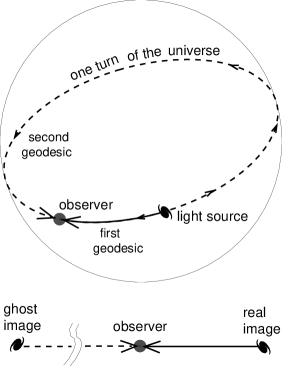
Figure 25: Ghosts of the second kind in a spherical (simply–connected) Universe.

In a MCM, there is in general no correspondence between $S_{obs}$ and a position in real space. But the correspondence between $S_{obs}$ and an event in spacetime does remain. Thus no one–to–one relation exists between $z$ (or $d_{obs}$) of an image and the distance of the corresponding emitting source in real space. To such a (unique) source, at a given position in space, are in general associated many images with different redshifts. This is due to the multi–connectedness of space, which implies that many spacetime geodesics link a spatial position to the observer (at present time).The nearest image is called “real” and the others are called “ghosts” (figure 26). Each image corresponds to a different null geodesic linking the source to us. To each of them is associated a set $S_{obs}$ of observable quantities.

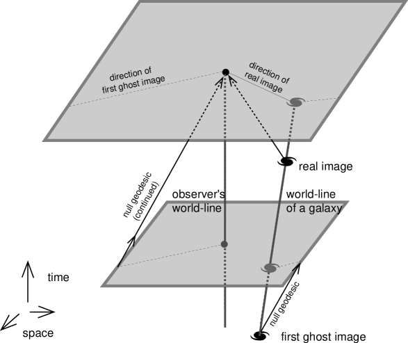
Figure 26: Real image and first ghost in a multi–connected universe.

To deal with this situation, it is convenient to work in the UC space : the one–to–one correspondence holds between $S_{obs}$ and a spatial position in the UC, which can be called the “observer’s world”. But the correspondence between these positions in the UC and those in real space is not univocal. In the UC, a different position is associated to each one of the bunch of geodesics linking an object in real space to the observer. Each of them corresponds to a ghost image of the real object, uniquely related to a geodesic and to the corresponding set $S_{obs}$ (figure 27). The unique image of the object which lies inside the fundamental cell and thus coincides with the original object, is called “real”. All observable properties of a ghost in the UC space identify to the properties of an object at the same position in the real space of the associated SCM (and linked by the same geodesic). All relations between $z$, the observable distance $d_{obs}$ and the look–back time hold exactly as in the corresponding SCM : to each redshift $z$ is associated an instant $t$ of emission, by the same formula $1+z=\frac{R_{0}}{R(t)}$ than in a SCM (which involves the curvature of spacetime), where $R_{0}=R(t_{0})$ is the present value of the scale factor. Most of the usual cosmological formulae may still be used, although they take their sense and validity in the UC, and not in the real space.

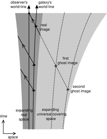
Figure 27: Different ghosts of the same galaxy in a multi–connected universe.

10.2 Comoving space and real space

In multi–connected models like in SCM’s, the geometry of space expands proportionally to the scale factor $R(t)$, in accordance to the Friedmann equations. Space at any time $t$ is exactly homothetic to space at any other time, for instance at the present time $t_{0}$, with the ratio $R(t)/R_{0}=1/1+z$. To any position $P$ in space at time $t$ corresponds, by the same homothety, a comoving position $P_{0}$ in the present space. To avoid comparisons of spatial properties at different times, all spatial positions of cosmic objects are considered in the comoving space. This is allowed by the fact that all spatial structures and relations, as well as the topology, are preserved by the homothety. For instance, rather than using the proper distance $d_{proper}(t)$ between 2 celestial objects at a time $t$, it is convenient to refer to their comoving proper distance $d_{proper}(t_{0})=(1+z)~{}d_{proper}(t)$.

This is still possible in the MCM’s. The geometry of space expands homothetically and all distances (including the dimensions of space itself) vary so. The homothety of ratio $\frac{1}{1+z}$ also preserves all topological properties. The UC at time $t$ is similarly imaged to the comoving UC. The relation between space and its universal covering is exactly identical to that between the comoving space and its comoving universal covering, and the comoving universal covering may be identified with the comoving space of the associated SCM. Thus the search for the topology of spacetime, already reduced to that of space, reduces further to that of the comoving space. Throughout this paper, if not specified otherwise, space will refer to comoving space, the universal covering will refer to the comoving universal covering, etc. Like in standard cosmology, all distances, volumes, densities,.. will be comoving quantities.

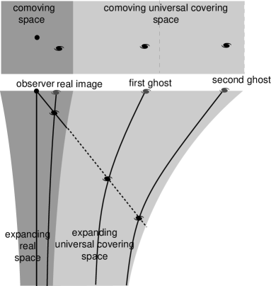
Figure 28: Ghosts in spacetime and in the universal covering.

10.3 Spatial scales

10.3.1 Hubble length

In SCM’s, the only scale related to comoving space is its curvature radius, identified to the present value of the scale factor $R(t_{0})=R_{0}$ (there is no scale at all in the flat case). Thus $R_{0}$ is the natural length unit in comoving space, and in the UC for a MCM. For instance, in the spherical simply–conected models, space has a finite volume $2\pi^{2}R_{0}^{3}$. The Friedmann equations imply the relation

$$\Omega+\lambda-1=\frac{k~{}c^{2}~{}}{~{}H_{0}^{2}~{}R_{0}^{2}}.$$ (41)

Unfortunately, the real value of $R_{0}$ remains unknown. The only cosmological length to which we have a direct observational access is the Hubble length

$$L_{Hubble}=cH_{0}^{-1}=3\,000~{}h^{-1}~{}\mbox{Mpc}.$$

If we define $f=\sqrt{\mid\Omega+\lambda-1\mid}$, we have for a non–flat universe  :

$$R_{0}=L_{Hubble}~{}f^{-1}=3\,000~{}(f~{}h)^{-1}\mbox{Mpc}.$$ (42)

Current observations imply $R_{0}>.5~{}L_{Hubble}$ and $R_{0}>L_{Hubble}$ if $\Lambda=0$ [10].

Another natural cosmological length is associated to the cosmological constant:

$$L_{\Lambda}=\sqrt{c^{2}/\Lambda}=1.17~{}10^{28}~{}\lambda^{-1/2}~{}h^{-1}~{}cm=400/\sqrt{\lambda}~{}h^{-1}~{}\mbox{Mpc}$$

.

10.3.2 Particle Horizon

The (present) particle horizon is the distance corresponding to an infinite value of the redshift :

$$L_{(z=\infty)}=R_{0}~{}\chi_{(z=\infty)}=c~{}R_{0}\int^{t=t_{0}}_{t=0}\frac{dt}{R(t)}.$$ (43)

It depends on the dynamics only. In standard cosmology (without inflation), the fact that the expansion law does not differ too much from a power law $R(t)\propto t^{\gamma}$ (with $\gamma\approx 2/3$ for matter dominated models) implies that

$$L_{(z=\infty)}=\chi_{(z=\infty)}~{}R_{0}\approx\frac{ct_{0}}{(1-\gamma)},$$ (44)

where $t_{0}=u~{}H_{0}^{-1}$ is the present age of the universe and $H_{0}^{-1}$ the Hubble time. In FL models, $u\approx\int^{1}_{0}dx~{}F(x),$ with $F^{-2}(x)~{}\equiv~{}\frac{\Omega}{x}+x^{2}~{}\lambda-\Omega-\lambda.$ In the Einstein–de Sitter solution ($\Omega=1$, $\Lambda=0$), $u=2/3$. More generally, $u<1$ if $\Lambda=0$ and remains of the order of unity for admissible models. It results that $L_{(z=\infty)}=R_{0}~{}\chi_{(z=\infty)}=\frac{u}{(1-\gamma)}~{}L_{Hubble}$, where $\frac{u}{(1-\gamma)}$ is of the order of unity (this is not the case, however, in models with inflation since the expansion does not follow a power law).

In any case, since the universe was opaque before the moment $t_{rec}$ of the recombination, the comoving length $L_{rec}=R_{0}~{}\chi_{rec}$ can be considered as a physical horizon, where

$$\chi_{rec}=c\int^{t=t_{0}}_{t=t_{rec}}\frac{dt}{R(t)}.$$ (45)

In models without inflation, $L_{(z=\infty)}$ and $L_{rec}$ almost coincide. In the case with inflation, $L_{rec}$ corresponds more than $L_{(z=\infty)}$ to the intuitive notion of horizon and represents with a good precision the (comoving) radius of the observable universe. Thus, to avoid any ambiguity, we define in the following $L_{h}=L_{rec}$ and $\chi_{horizon}=\chi_{rec}$. It results that in all cases (with or without inflation),

$$\chi_{horizon}\approx\frac{u~{}f}{(1-\gamma)}$$

and $L_{h}\approx\frac{u}{(1-\gamma)}~{}L_{Hubble}=3\,000~{}\frac{u}{(1-\gamma)}~{}h^{-1}~{}\mbox{Mpc},$ where $u$, $f$ , $h$ and $1-\gamma$ are of the order of unity.

The concept of horizon keeps its exact validity in the MCM’s, but must be applied to the universal covering space : an image is potentially visible iff its (comoving) distance is smaller than $L_{h}$ in the universal covering. This sets a priori no constraint about the position of the real object. A particle horizon can be similarly defined at any epoch $t$, from eq.(43) where the upper bound of integration $t_{0}$ is replaced by $t$.

In the non flat case, topological constraints impose precise relations between the dimensions of space compared to the radius of curvature. On the other hand, the potential visibility of ghosts images is linked to their situation with respect to the horizon. Thus $\chi_{horizon}$, the ratio of the horizon length over the curvature radius has to be maximum if observable effects are expected. Figure 29 displays $\chi_{z=\infty}$ (for a standard Friedmann–Lemaître model) as a function of the cosmic parameters $\Omega$ anf $\lambda$.

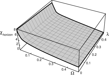
Figure 29: The horizon length in curvature radius units.

10.3.3 Spatial scales associated to multi–connectedness

In a MCM, additional spatial scales are associated with the topology, those of the fundamental polyhedron. The geometry suggests to compare them with $R_{0}$ but it is often more convenient, for observations, to compare them to $L_{Hubble}$ or $L_{h}$, or to evaluate them in Mpc or $h^{-1}~{}\mbox{Mpc}$. Observable effects linked to the multi–connectedness will only occur if these scales are smaller than the size of the observable universe, i.e., the horizon length. We call $\alpha$ the smallest length associated with the fundamental polyhedron. As already mentionned, the ratio $\alpha/R_{0}$ can only take specific values in a non flat space : when $k>0$ (resp. $k<0$), the geometry imposes a maximum (resp. minimum) value for it. It remains arbitrary in flat space. An other scale is involved, the maximum length $\beta$ inscriptible in the fundamental polyhedron, which is also the diameter of the sphere inscribing it. $\beta$ is also the maximum distance between 2 images of the same object belonging to adjacent cells. $\alpha/2$ and $\beta/2$ are the minimum and the maximum distance of the observer, assumed at the center of the fundamental polyhedron, to its boundaries.

For instance, the geometry of the 3–torus (figure 30) is defined by the 3 lengths $\alpha_{x}$, $\alpha_{y}$ and $\alpha_{z}$, with $\alpha=min(\alpha_{x},\alpha_{y},\alpha_{z})$, the length of the smallest side, and $\beta=\sqrt{(\alpha_{x})^{2}+(\alpha_{y})^{2}+(\alpha_{z})^{2}}$, the length of the diagonal. If real space has the topology of such a 3–torus, immediate observations impose that $\alpha$ cannot be too small, for instance smaller than the size of the Milky Way. The observations detailed in the next sections allow to increase this lower limit.

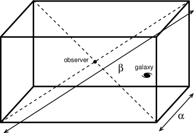
Figure 30: Characteristic lengths of a toroidal universe.

10.4 Multi–connected universes with flat spatial sections

For simply or multi–connected models, space is Euclidean if $\Omega+\lambda=1$. The universal covering is ${\rm I\!R}$³ and space has no characteristic scale : the present value $R_{0}$ of the scale factor may be chosen arbitrarily and thus cannot be used as an intrinsic length unit. A convenient metric is (37) with $S_{0}(\chi)=\chi$. The variety of topological spaces with flat curvature has been detailed in §6. Among the non compact models (where space is infinite in at least one direction, so that $\beta=\infty$), three types, beside ${\rm I\!R}$³ itself, are orientable and thus are candidates for MCM’s. Since they are non compact, they have been less discussed in the litterature. In many aspects, their properties are intermediary between those of SCM’s and those of, for instance, the torus. Thus, for the cosmological purpose it is especially interesting to consider the 6 kinds of orientable closed spaces with constant flat curvature described in §6.

The 3 dimensional hypertorus $T^{3}$ is the simplest case. Its fundamental cell is a parallepiped with 3 arbitrary dimensions $\alpha_{x},\alpha_{y}$, and $\alpha_{z}$. Its principal directions define 3 preferred orientations in space, thus breaking the global isotropy. This is a general property of multi–connected models. For this space, there is no mathematical constraint on the values of $\alpha$, the smallest side of the FP, and $\beta$, its diagonal. Multi–connected universe models with toroidal space have been widely studied. For instance all the images of an object lying onto one of the principal directions are distributed with a periodicity in comoving proper distance. This has motivated observational searches for periodicities. On the other hand, the hypertorus produces some images of the observer which could be potentially visible in opposite directions (if they are within the horizon). This has also motivated specific searches that we present in §11.5.1.

Cosmological models where the fundamental polyhedron is paralellepipedic, but where faces are twisted before identifications would appear, in some aspects, alike the hypertorus. It should be mentionned that, in the case where the faces are rotated by $\pi/2$, the arbitrariness is reduced because of the additional condition $\alpha_{x}=\alpha_{y}$ necessary to allow for the identification. Models based on a fundamental cell with hexagonal faces have not been studied to our knowledge.

10.5 Multi–connected universes with positive spatial curvature

In this case, the UC – the 3–sphere   $\textstyle\rm S$³ – is compact, so that all models also have compact spatial sections. The present radius of the universe $R_{0}$ is chosen to coincide with the curvature radius of (comoving) space.   $\textstyle\rm S$³ is advantageously described with the comoving metric (37) with $S_{1}(\chi)=sinh(\chi)$. Its whole extent is described by $\chi$ from $0$ to $\pi$ , $\phi$ from $0$ to $2\pi$ , and $\theta$ from $0$ to $\pi$.

10.5.1 The elliptical space

As soon as 1917, de Sitter [25, 26] distinguished the spherical space   $\textstyle\rm S$³ and the projective space ${\rm I\!P}$³ that he called the elliptical space. Then he compared the properties of cosmological models based on these two spatial parts. For instance they have for respective (comoving) volumes $2\pi^{2}~{}R_{0}^{3}$ and $\pi^{2}~{}R_{0}^{3}$. The maximum distance between 2 points is $\pi R_{0}$ in   $\textstyle\rm S$³ and $\pi R_{0}/2$ in ${\rm I\!P}$³. But the main difference to his eyes was due to the presence, in   $\textstyle\rm S$³, of an antipodal point associated to any point, and in particular to the observer, at a distance of $\pi~{}R_{0}$ precisely. To avoid this undesirable fact, he claimed that cosmological models with ${\rm I\!P}$³ are much preferable than those with   $\textstyle\rm S$³ and he mentionned that Einstein had the same opinion. Since both spaces are, for a given value of $R_{0}$, of approximatively the same size (only a factor 2), it would be very difficult to decide from observations in which we live, if it appeared that $\Omega+\lambda>1$. In this case, if we follow Einstein and de Sitter, ${\rm I\!P}$³ would be a better assumption than   $\textstyle\rm S$³.

However, de Sitter correctly remarked that, for admissible values of $\Omega$ and $\lambda$ it is probable that the most remote points lie beyond the horizon, so that the antipodal point, if any, would remain unobservable. Eddington [30] also referred to elliptical space as an alternative as much as attractive as   $\textstyle\rm S$³. His discussion for comparing both models led him to very interesting discussions about the nature of space. He pointed out for instance that many conceptual difficulties arose from the fact that space is often, and erroneously, considered as a “continuum in which objects are located”. He suggested then to abandon this misconception and to consider space as a network of intervals. In this case, the structure of the whole space appears only as the lattice–structure of all cross–connexions between points. We will not here go deeper into these discussions but only point out again that there is no simple argument according to which space should be simply–connected. Friedmann [62] and Lemaître [95] also discussed these possibility and preferred the elliptical form of closed space for aesthetical reasons.

Narlikar & Seshadri [115] examined the conditions in which ghost images of celestial objects may be visible in a Friedmann–Lemaître model with elliptical space. They suggested that, in such a model the apparent cutoff in the redshift distribution of quasars may be due to this effect (see §11.5).

10.5.2 Lens spaces and similar MCM’s

None of these authors mentionned other multi–connected spaces in a cosmological context. This was done by Gott [72]. For instance, the rotations of the cyclic group $Z_{n}$ ($n>2$) (see §7) generate MCM’s where space is   $\textstyle\rm S$${}^{3}~{}/~{}Z_{n}$. The larger the value of $n$, the smaller the dimensions of space. The simplest, and largest, case is the lens space $M={\mathchoice{\hbox{\raise 3.41666pt\hbox to0.0pt{\kern 1.94447pt\vrule height=3.07497pt\hss}\hbox to0.0pt{\kern 3.05557pt\vrule height=3.41666pt\hss}\hbox{$\displaystyle\rm S$}}}{\hbox{\raise 3.41666pt\hbox to0.0pt{\kern 1.94447pt\vrule height=3.07497pt\hss}\hbox to0.0pt{\kern 3.05557pt\vrule height=3.41666pt\hss}\hbox{$\textstyle\rm S$}}}{\hbox{\raise 2.39166pt\hbox to0.0pt{\kern 1.36113pt\vrule height=2.15248pt\hss}\raise 0.23917pt\hbox to0.0pt{\kern 1.94444pt\vrule height=2.15248pt\hss}\hbox{$\scriptstyle\rm S$}}}{\hbox{\raise 1.70833pt\hbox to0.0pt{\kern 1.11108pt\vrule height=1.53748pt\hss}\raise 0.17084pt\hbox to0.0pt{\kern 1.52779pt\vrule height=1.53748pt\hss}\hbox{$\scriptscriptstyle\rm S$}}}}$${}^{3}/Z_{3}$, which tesselates   $\textstyle\rm S$³ into 6 replicae of the fundamental cell having a lens form. In the corresponding MCM, an observer (at $\chi=0$) has 5 images of itself, whose coordinates are given in §7. The minimum distance between images is $\alpha=\pi R_{0}/3$ and the maximum dimension of the fundamental lens is $\beta=\pi R_{0}/2$. Gott remarked that in a standard Friedmann–Lemaître model, this is larger than the size of the horizon, so that no observable effects would take place in such MCM’s. Interesting cases for observational cosmology involve fundamental cells of smaller sizes, and thus higher values of $n$.

The dihedral group $D_{m}$ ($m>2$) gives the spaces   $\textstyle\rm S$${}^{3}/D_{m}$. For instance, $D_{3}$ generates 11 images of the observer (coordinates in §7). MCM’s can also be constructed from the polyhedral groups : $T$ divides   $\textstyle\rm S$³ into 24 tetrahedral quotient spaces, with observer’s nearest image at a distance $\alpha=\pi R_{0}/3$. $O$ divides   $\textstyle\rm S$³ into 48 octahedral quotient spaces, with observer’s nearest image at $\alpha=\pi R_{0}/4$. $I$ divides   $\textstyle\rm S$³ into 120 dodecahedral quotient spaces, with observer’s nearest image at $\alpha=\pi R_{0}/5$. For this latter case, Gott showed that the fundamental cell may be inscribed in a sphere of radius $\beta/2=0.338~{}R_{0}$.

The spaces   $\textstyle\rm S$${}^{3}/Z_{n}$ and   $\textstyle\rm S$${}^{3}/D_{m}$ with small values of $n$ or $m$ have dimensions comparable to $R_{0}$ or to the horizon length. This is also true for   $\textstyle\rm S$${}^{3}/T$,   $\textstyle\rm S$${}^{3}/O$ and   $\textstyle\rm S$${}^{3}/I$. In any case $\beta$ remains always greater than $0.326~{}R_{0}$, the value for ${\mathchoice{\hbox{\raise 3.41666pt\hbox to0.0pt{\kern 1.94447pt\vrule height=3.07497pt\hss}\hbox to0.0pt{\kern 3.05557pt\vrule height=3.41666pt\hss}\hbox{$\displaystyle\rm S$}}}{\hbox{\raise 3.41666pt\hbox to0.0pt{\kern 1.94447pt\vrule height=3.07497pt\hss}\hbox to0.0pt{\kern 3.05557pt\vrule height=3.41666pt\hss}\hbox{$\textstyle\rm S$}}}{\hbox{\raise 2.39166pt\hbox to0.0pt{\kern 1.36113pt\vrule height=2.15248pt\hss}\raise 0.23917pt\hbox to0.0pt{\kern 1.94444pt\vrule height=2.15248pt\hss}\hbox{$\scriptstyle\rm S$}}}{\hbox{\raise 1.70833pt\hbox to0.0pt{\kern 1.11108pt\vrule height=1.53748pt\hss}\raise 0.17084pt\hbox to0.0pt{\kern 1.52779pt\vrule height=1.53748pt\hss}\hbox{$\scriptscriptstyle\rm S$}}}}^{3}/I$. In these cases, where ghost images would be at distances comparable to the horizon, very few observable effects can be expected. On the other side, very large values of $m$ or $n$ would lead to identification lengths so small that they are excluded by the present observations (see below). The most interesting cases would therefore lie in the intermediate range.

10.6 Multi–connected universes with negative spatial curvature

When the covering space is ${\rm I\!H}$³, the scale factor $R_{0}$ may be chosen to coincide with the radius of curvature, and may be used as a unit length. The metric is usually written under the comoving form (37) with $S_{-1}(\chi)=\sinh\chi$. The coordinate $\chi$ varies from $0$ to infinity, $\theta$ and $\phi$ from 0 to $2\pi$. An infinite number of MCM’s with negative spatial curvature may be build by various means as depicted in §8.

Symmetrically to the case of constant positive curvature, where the volume of a manifold is an entire fraction of $2\pi^{2}~{}R_{0}^{3}$ which is thus an upper bound, there is a minimal value $vol_{min}$ for the volume of a manifold with constant negative curvature (see §8). Its value remains however unknown, and it is not known either if there is a minimum value for $\alpha$. We decribe in §10.6.4 models where space could have a volume equal to $vol_{min}$. Given this constraint, the most interesting models for cosmology are those with the maximum ratio $L_{h}/R_{0}$, i.e., low values of $\Omega$ and, to a lesser extent, of $\lambda$, as it appears in figure 29.

10.6.1 A toy spacetime in 3–dimensions

A 3–dimensional universe model introduced by Fagundes [43, 44, 46] presents a pedagogical interest. Its (two–dimensional) spatial part is the 2–$torus$ $T_{2}$, whose fundamental polyhedron  is a regular octogon as described in §3.2.1 and §4.3.3.

This 3–dimensional spacetime admits the metric

$$ds^{2}=a(\eta)^{2}(d\eta^{2}-d\sigma^{2}),$$ (46)

a restriction of the Kantowski–Sachs metric (23). In this formula, $a(\eta)=R(t)$ is the scale factor, with present value $a_{0}=R_{0}$ and $\eta$ is the conformal time defined by $a(\eta)~{}d\eta=cdt$ which becomes, after integration, $ct=a_{0}~{}(\sinh\eta-\eta)$. The spatial part of the metric

$$R^{2}~{}d\sigma^{2}=R^{2}~{}(dr^{2}+\sinh^{2}r~{}d\phi^{2})$$ (47)

has a negative curvature $-1/R^{2}(t)$.

The comoving space, with a curvature radius $R_{0}$, is described by the metric $R_{0}^{2}~{}d\sigma^{2}$. Although the model does not intend to represent the real universe, Fagundes [46] derived the coordinate of the horizon $\eta_{horizon}\approx 6$, corresponding to a distance $\approx 6~{}R_{0}$. The redshift of a source at a coordinate distance $r_{1}$ is given by : $1+z_{1}=\frac{a_{0}}{a(\eta_{1})}$, with $\eta_{1}=\eta_{0}-r_{1}$. The distance between 2 adjacent images, equivalent to the length of the smallest geodesic loop in $T_{2}$ is $\alpha\approx 3~{}R_{0}$. The nearest image of a source appears about halfway to the horizon, thus very far away. This illustrates that the fundamental cell cannot be made very small in a MCM’s with negative curvature. Fagundes emphasized this by calculating that a source at redshift $z=0.7$ would have its first image at $z=$42. The purpose of his paper was mainly pedagogical, to illustrate how multiple images and counter images of quasars could occur, with the idea that this could solve the quasar redshift controversy. We present the 4–dimensional generalisation of his model [49] in §10.6.3, and we discuss the implications of multi–connectedness onto the quasar distribution in §11.5.

10.6.2 Non–compact models

Some examples of non compact multi–connected hyperbolic spaces were presented in §8.4. There is a general procedure which allows to build such a space ${\rm I\!H}^{3}/\Gamma$ from a multi–connected surface ${\rm I\!H}^{2}/\Gamma$ : it is non compact in the direction orthogonal to ${\rm I\!H}^{2}/\Gamma$.

Gott [72] applied this procedure, tesselating ${\rm I\!H}^{2}$ with regular n–gones. According to a theorem of hyperbolic geometry, their area is $R_{0}^{2}$ times the angle deficit [$\pi(n-2)$ - the sum of all angles at vertices]. For instance the octogon in ${\rm I\!H}^{2}$ has all angles $=\pi/4$, and a surface $4\pi R_{0}^{2}$. Then the identification of the sides 1 with 3, 2 with 4, 5 with 7 and 6 with 8 gives to each octogon the topology of a sphere with 2 handles.

This may be generalized to $n$–gons ($n=4g$), which have the topology of a sphere with $g$ handles. Thus ${\rm I\!H}$² can be tesselated with cells topologically equivalent to spheres with $n$ handles. The one considered by Gott has its fundamental polyhedron formed from 2 regular tetrahedra with vertices at infinity, which are glued together. It is non compact.

Another MCM with non compact hyperbolic space was considered by Sokoloff and Starobinskii [143]. Its spatial part is the “cylindrical horn” described in §• ‣ 8.4.1. In the frame of this model they studied the structure and the growth of the density–perturbations which could have led to the formation of galaxies, clusters, etc. Those are discussed in §12.2.2.

10.6.3 Compact models

The topologies of ${\rm I\!H}^{3}$ which give observable effects are those having the smallest fundamental polyhedron as possible (in analogy to the high $n$ or $m$ modes in the spherical case). We list below the main MCM’s constructed from one of the compact manifolds ${\rm I\!H}$${}^{3}/\Gamma$

• Gott [72] proposed a model whose spatial part is the Löbell space [98], described in §21. He calculated $\alpha=2.64~{}R_{0}$ and showed that the present horizon contains no more than about 10 replicae of the fundamental polyhedron. The Löbell space is thus too large to give interesting observable effects. Considering the time evolution, he showed that the entire space entered the cosmological horizon at a redshift $z\approx 6$ (this is defined as the first moment where the whole space, whose proper volume increases $\propto R^{3}(t)$, is contained within the horizon).

• Fagundes [45] studied a “quasi–hyperbolic” model where space has the topology of $T_{g}~{}*~{}S^{1}$. Here $S^{1}$ is the ordinary circle, parametrized by the coordinate $\zeta$ and $T_{g}$ is the $g$–torus, described by the 2 coordinates $\rho$ and $\phi$. It should be emphasized that the universal covering space is not ${\rm I\!H}^{3}$ but the product ${\rm I\!H}^{2}\times{\rm I\!R}$. This space, being anisotropic, has therefore no constant spatial curvature. This model generalizes the 2–dimensional study of §10.6.1.

  This MCM may be described by the Kantowski–Sachs metric (23)

  $$ds^{2}=c^{2}dt^{2}-R^{2}(t)~{}(d\rho^{2}+sinh^{2}\rho~{}d\phi^{2})-b^{2}(t)~{}d\zeta^{2}.$$ (48)

  It can be also written in the conformal Robertson–Walker form :

  $$ds^{2}=a(\eta)^{2}~{}(d\eta^{2}-d\sigma^{2})=c^{2}~{}dt^{2}-R^{2}(t)~{}d\sigma^{2},$$ (49)

  where $a(\eta)=R(t)$ is the scale factor, with present value $R_{0}$, $\eta$ the conformal time defined by $a(\eta)~{}d\eta=c~{}dt$, and $R~{}d\sigma$ the spatial metric.

  Solving the Einstein equations for a dust–filled Universe, Fagundes derived the parametrized solution :

  $$ct=R_{0}~{}(\sinh\eta-\eta),$$

  $$a(t)=R_{0}~{}(cosh\eta-1),$$

  $$b(t)=3R_{0}~{}(\eta~{}cosh\frac{\eta}{2}-2).$$

  Restricting his discussion to the 2–torus ($g=2$), Fagundes explored some properties of the Cosmic Microwave Background, that we describe in see §12.

• Fagundes [49, 48] also studied models where space is a Best model [11]. The Best spaces (see §22) have one of the topologies ${\rm I\!H}^{3}/I$, where $I$ is the regular icosahedron.

  Fagundes [49] investigated the dynamical properties with the parameters $\Omega=0.1$ and $\Lambda=0$. The redshift $z_{1}$ of a source at a coordinate distance $\chi_{1}$ is given by : $1+z_{1}=\frac{R_{0}}{a(\eta_{1})}$, with $\eta_{1}=\eta_{0}-\chi_{1}$. Fagundes calculated the 20 generators of the holonomy groups which transform any source, in the fundamental polyhedron, into 20 images in the adjacent cells, and more beyond. He remarked that images of the center of the fundamental polyhedron are given, in the universal covering ${\rm I\!H}^{3}$, by reflexions on the 20 faces of the fundamental polyhedron.

  Fagundes was interested in the existence of multiple images of a given source, with a main focus towards our own Galaxy, the Milky Way. He calculated the positions of ghost images with a method similar to the ray–tracing procedure used to synthetize realistic images by computer. He emphasized the existence of conjunctions (or oppositions and other associations) of images onto the sky. He discussed in particular a case where the original source has a redshift of 0.124, the conjunct of 4.263, and associated images of 3.14, 2.34, and 1.94. In his opinion, they could be good candidates for the discordant quasar associations. We discuss these topics in sections 11.3 and 11.5.

10.6.4 The minimum volume model

As we mentionned in §8, the possible values of the volume of a space with constant negative curvature are bounded from below. But the limiting value $vol_{min}$ remains unknown. Weeks [154] and Matveev & Fomenko [107] found the manifold with the minimum volume presently known, i.e., 0.94 $R_{0}^{3}$, which is described in §8.4.2. On the other hand Meyerhoff [109] demonstrated that $vol_{min}>V_{Meyerhoff}=0.00082~{}R_{0}^{3}$. Recently, Hayward & Twamley [83] have studied multi–connected models based onto the Weeks–Matveev–Fomenko manifold. They considered, in this framework, the possible isotropization of the Cosmic Microwave Background (see §12) and tried to explain the apparent periodicity in the galaxy distribution found by Broadhurst et al.  [15]. Although there is no known manifold corresponding to the volume $V_{Meyerhoff}$, they made the hypothesis that there could exist one and guessed the possible properties of a universe having it as a spatial part. For these 2 manifolds respectively, they considered a (hyperbolic) sphere having the volume of the whole space and considered its diameter $L_{max}$ as an upper bound for $\alpha$. For the 2 models they found respectively the values

$$L_{max,WMF}=\frac{3552}{\sqrt{1-\Omega}}~{}h^{-1}~{}\mbox{Mpc}$$ (50)

and

$$L_{max,Meyerhoff}=\frac{348}{\sqrt{1-\Omega}}~{}h^{-1}~{}\mbox{Mpc}.$$ (51)

Comparing these expressions to the present observational limits derived from the observations of galaxy clusters (see §11.4), they concluded that both manifolds are presently admissible.

10.6.5 Barrel models

Most observational tests could concern only local parts of the universe, i.e., at distances much smaller than the curvature radius of space. At these scales curvature effects play no role. Thus Sokoloff [143, 135] remarked that all compact MCM’s, with negative spatial curvature, have the same asymptotic structure. To describe this he employed the Euclidean metric, approximately valid for scales not too large, in polar coordinates $x$, $r$, $\phi$. Then the considered MCM’s correspond to the “barrel structure” defined by the identifications :

$$x=x+n~{}h$$

and

$$\phi=\phi/n~{}a,$$

where $n=$0, 1, 2,… $h$ is a constant identification length and $a$ an identification angle ($a=0$ corresponds to cylindrical space). A MCM with negative spatial curvature would look very alike such a barrel space. Such models are of course anisotropic with the $x$–axis as a preferred direction (or $a=0$). They were studied [143, 135] in relation with cosmic magnetic fields (see §12.4).

11 Ghosts in multi–connected Universes

The hypothesis that the real universe is multi–connected has various implications. On one hand, if the identification scale is of the order of the horizon or larger, no directly observable effect is expected, although primordial quantum effects could have generated interesting effects. On the other hand, if the topological scales $\alpha$ and $\beta$ are significantly smaller than the present horizon, observable effects will be manifest, among which the most interesting is the existence of ghost images. We will concentrate now on the “small universes”, defined as those where $\alpha<L_{h}$, of the order of a few 100 or 1 000 Mpc. Our knowledge of the universe gets worse when the spatial scale increases, with the horizon as a limit. Thus, the smaller the basic cell (i.e., the fundamental polyhedron, which identifies with the real space) the easier are topological effects to observe. How do the present observational data constrain the possible multi–connectedness of the Universe ? And, more generally, what kinds of tests are conceivable ? These questions are developed in this section and the following ones. We will also discuss the suggestions that multi–connectedness of the Univers could explain some observational results not presently understood, like discordant redshift associations, redshift periodicity, distribution of the gamma ray bursts,…

11.1 Geodesics and ghosts

The topology of a given Friedmann–Lemaître model is characterized by the shape and the dimensions of the fundamental polyhedron. The simplest case of the torus $T^{3}$, for instance, corresponds to a parallelepiped with 3 identification lengths $\alpha_{x},\alpha_{y}$ and $\alpha_{z}$. We refer as $\alpha$ and $\alpha_{max}$ respectively to the smallest and the largest of these lengths (see §10.3). Sokoloff & Shvartsman [142] have defined the characteristic radii $R_{1}$ and $R_{2}$ : by definition, there is no ghost image of a source nearest than $R_{1}$ to the observer, so that $R_{1}=\alpha/2$ (figure 30). Also, by definition, no single original source lies beyond $R_{2}$, which appears therefore as the radius of the smallest sphere containing entirely the fundamental cell : $R_{2}=\beta/2$, where $\beta=(\alpha_{x}^{2}+\alpha_{y}^{2}+\alpha_{z}^{2})^{1/2}$ is the diagonal. The real image of any celestial object is always closer than $\beta/2$ to the Earth. The torus considered by Gott [72] has all fundamental lengths equal to $\alpha=28.5~{}h^{-1}~{}\mbox{Mpc}$, so that $\beta=50~{}h^{-1}~{}\mbox{Mpc}$ (note that he calls $R_{H}$ the quantity $\beta/2$). In the more general case, the relation between $\beta$ and $\alpha$ depends on the geometry.

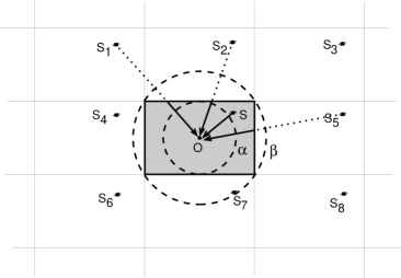
Figure 31: Multiplication of images in the universal covering space of a toroidal universe.

In a MCM, many null geodesics start from the position of an object (e.g., a light source) in real space, to reach the present observer (figure 31). They represent light rays which have been emitted at different epochs. To each of them corresponds a set $S$ of observable quantities (see §10.1), and an image of the real object. These images, replicae of the original object in the universal covering, are called “ghosts” and can be labelled by an index $i$. All these images have the same status but a region of the universal covering is arbitrarily chosen to match the (multi–connected) real space. This “real part” of the universal covering, the basic cell, is generally chosen to coincide with the fundamental polyhedron centered on the observer, although this choice is for pure convenience in homogeneous models. Then, the unique image situated in this real part of the universal covering is called the real object and all other will be called ghosts. In the following we will assume with no loss of generality (when space is homogeneous) that the observer lies at the center of the fundamental polyhedron.

The ghosts are images of a real object, so that their associated proper (comoving) distances, in space, are rigorously identical to $\hat{d}$, that of the original (not taking into account its possible proper motion during the light–crossing–time). But instead of the proper distance, measurements provide other observable distances $d_{obs}$ (the luminosity–distance, the angular–diameter distance, the parallax–distance, etc.) of the ghosts. In general the values of $d_{obs}$ differ from a ghost to another of the same object. As we mentioned earlier, $d_{obs}$ is to be interpreted as a distance in the universal covering space. Work in the universal covering rather than in real space thus allows us to conserve the usual cosmological interpretation of all distances. In the universal covering, it is also possible to assign a proper (comoving) distance $d_{i}>\alpha/2$ to each ghost (only the original image has $\hat{d}=d<\alpha/2$; conversely, only ghosts are observed at $d>\beta/2$). The ghosts are in general observed with different redshifts $z_{i}$. The holonomies which define the topology are isometries of the comoving universal covering space, and thus concern the proper comoving distances $d_{i}$.

The most natural way to prove that our universe is multi–connected would be to show, ponctually or statistically, the existence of ghost images of objects or of specific configurations. In the following we present different methods which have been, or which can be applied in this purpose. The number of potential ghosts of an object equals the ratio of the volume of the universal covering space to that of the fundamental polyhedron, and thus depends on the cosmic parameters and on the topology considered : it is finite in the case of positive constant spatial curvature, infinite otherwise. Only ghosts nearer than the horizon can be seen, so that their number is reduced to the number of cells in the observable universe, i.e., about $L_{h}^{3}/(\alpha\beta)^{3/2}$, where $(\alpha\beta)^{3/2}$ is a rough estimate of the volume of the fundamental polyhedron.

The distinct null geodesics associated to different ghosts of a same object correspond to different look–back times (defined as the temporal delay between emission and reception of the radiation) and redshifts. This would allow to distinguish ghosts of the same object, appearing on very close lines of sight (or on the same one), from multiple images created by gravitational lensing, which have equal redshifts and look–back times. For a ghost, all usual cosmological relations hold when they involve distances or quantities estimated in the universal covering. In particular, the larger this distance, the longer the look–back time and the redshift (both larger than for the original image, the nearest in the universal covering). The more distant a ghost in the universal covering, the younger appears the corresponding object. For instance, a ghost of the Sun could unveil its aspect millions or billions years ago.

The differences in the look–back times for ghosts of a same object correspond to the time necessary for light to made different numbers of turns around the universe. Thus they appear approximatively as multiples or combinations of the $\alpha_{i}/c$. But cosmic objects have a finite lifetime. For an object with an intrinsic lifetime $T$, the number of visible ghosts is limited to $\approx(cT)^{3}/(\alpha\beta)^{3/2}$. Too distant (resp. near) ghosts would correspond to a time of emission when the object was not yet (resp. no more) existing. This limits the possible observation of ghosts to objects with lifetime $T\geq\alpha/c$. This is crucial for quasars, that we discuss in §11.5.

Moreover, even if an object does exist during a long period of time, this does not guarantee that it will be easily recognizable. For that, it would be also necessary that its appearance has not changed too much during its lifetime. Thus the tests must be performed on objects which live long enough, and which keep a sufficiently constant aspect during their life.

11.2 Searching for ghosts

The usual cosmological relations hold in the universal covering : the more distant a ghost, the weaker its luminosity, the smaller its angular size (the possible reconvergence of geodesics due to the spatial curvature is avery large scale effect which plays no role in current observations). Very distant ghosts cannot be observed for the same reasons than distant objects in the SCM’s. Observing techniques define a practically usable portion of space, inside which a ghost remains observable and recognizable, depending on the type of objects (or configurations) considered, and of the observation procedure. This limits again the number of observable ghosts. In addition some peculiar reason may forbid to observe a ghost visible in principle : an high obscuration region, or an other object ahead on the line of sight can mask it. It results that no test which depends on the observation of a small number of ghosts only can be used to rule out a MCM, since the non–observation of an expected ghost could be attributed to many different reasons.

Additional effects may also perturb the observation of ghosts. Because the Universe is not exactly homogeneous, the null geodesics are not exactly those of the spatially homogeneous spacetime. They are deformed by the density inhomogenities, leading to the various consequences of gravitational lensing : deformation, amplification, multiplications of images… A ghost so amplified, or distorted, may become hard to recognize. The expected effect is however rather weak in typical conditions : the maximum angular displacement of a distant source can be estimated to be less than $1^{\prime}$ for lensing by a cluster of mass $\approx 2~{}10^{13}~{}M_{\odot}$ and dimensions $\approx~{}$3 Mpc. In a MCM, however, there is also a non zero probability that the light from a ghost is gravitationnally distorted by the object itself (this is expected when the object lies in a principal direction). Such configurations have not been considered up to now at our knowledge, although they could give raise to curious effects. In general, however, the expected influence of gravitational lensing is weak enough to be neglected [27].

Finally, proper velocities, which reach typically $V_{p}\approx 500$ km s^-1 or more for cosmic objects, must be taken into account. During a time $\approx\alpha/c$, when a light ray turns around a small universe, the real object moves by $\approx V_{p}~{}\alpha/c$. Thus the position of the next ghost, in the UC, is shifted by the corresponding angle, typically a few arcminutes. For this reason, any search for ghosts must be performed with a finite spatial resolution of this order.

The simplest conceivable test is the search for possible ghosts of a specific class of objects : individual galaxies (possibly with some peculiar characterisitics); clusters, superclusters or peculiar associations of galaxies; quasars, active galactic nuclei, or radiosources; and more generally any type of recognizable systems, like for instance peculiar associations of objects (chains, rings, voids,…). The first attempts were devoted to the search for ghost(s) of an individual peculiar object : the Milky Way or another typical galaxy, the Virgo and Coma clusters, the Local Supercluster, etc. Further studies, that we also describe in the next sections, have been devoted to the search of peculiar configurations (coincidences, oppositions, or other) or of periodicities of images on the sky.

11.3 Ghost images of individual galaxies

A fascinating possibility, in a sufficiently small universe, lies in the fact that ghost images of our own Galaxy should be visible (thus, from outside). Their number, distances and orientations depend on the topology. The nearest must be at a distance $\alpha/2$. So, not seeing any image of our Galaxy up to a distance $d$ would allow us to exclude topologies with $\alpha<2d$. A sphere of radius $R$ in the universal covering contains between $(\frac{2R}{\alpha})^{k}$ and $(\frac{2R}{\beta})^{k}$ images, where $k$ is the number of principal directions. The maximum distance $d$ up to which we would be able to recognize our galaxy has been discussed by Sokolov and Shvartsman [142]. They deduce that $d>7.5~{}h^{-1}$  Mpc, implying $\alpha>15~{}h^{-1}$ Mpc (see also [48, 52]). However, many galaxies are visible in the sky and there is no simple way to decide if such observed galaxy may be or not a ghost image of the Milky Way. It would thus be very difficult to decide in this way if we do, or do not, live in a MCM.

The main interest offered by the Milky Way comes from its situation at the node between the principal directions (in a homogoneous MCM), so that it lies automatically on each of them. This implies an exact quantization, in proper comoving distance, of its ghost images : series of images of our Galaxy should appear in the principal directions, having for proper comoving distances entire multiples of $\alpha_{i}$, the distance to the first ghost in this direction. This equality must be considered with a spatial resolution depending on our proper motion, see §11.2. Also, most MCM’s predict that, if a ghost is present in one direction, an other must be present in the opposite direction at similar distance and redshift. Some MCM’s also predict ghost images in perpendicular (or in other well defined) directions. Thus the observation of similar images at identical redshifts, and in related (preferentially opposite, or perpendicular) directions, is expected in a MCM. This would also be the case if images are observed in a common direction with quantized comoving distances. To apply this latter test, it remains to decide what kind of image must be searched for, or in other words, what was the appearance of the Milky Way some millions years ago. Fagundes & Wichoski [52], following an ealier suggestion by Lynden–Bell, proposed that our galaxy was a quasar a long time ago. In this case, any observed quasar could a priori  be a ghost image of the Milky Way. We present in §11.5 their search for quasar–images in opposite or related directions on the sky.

Fagundes [49] examined the occurence of images of the Milky Way in the MCM decribed in §10.6.3, where space is the Best model. The large number of principal directions makes this peculiar geometry especially favorable. For this model, Fagundes was able to show that several conjunctions between source and images should be expected, in specific regions of the sky distributed along an equatorial band. The situation would however not be so favorable for other models. Thus, although he expressed the hope that discordant redshifts could be accounted for in this way (see §11.5.2), no firm conclusion may be drawn from these studies.

Presently, no source has been recognized as an image of our Galaxy and this search has failed to provide interesting limits : the derived constraints are much weaker than those derived from other types of objects. It remains thus very few hope to use the Milky Way to test in any way the hypothesis of multi–connectedness.

Multi–connectedness would also imply the presence of several ghost images of any individual galaxy. Demianński & Lapucha searched for instance, without success, opposite images of galaxies in the sky. However, as stated by Sokoloff & Shvartsman [142], it would be very difficult to recognize that different galaxies are indeed images of an unique one. Moreover, the spatial coverage of galaxies does not extend very far away, so that, compared to the other possibilities, galaxies do not appear as good candidates to test the multi–connectedness of the universe.

11.4 Ghost images of clusters and superclusters

The brighter – and the more recognizable – a type of objects, the greater interest it offers for testing multi–connectedness. Sokoloff & Shvartsman [142] examined clusters of galaxies. Contrarily to, e.g. , quasars, the lifetimes of clusters seem sufficiently long to guarantee an appearance almost constant during the time necessary for light to cross a small Universe. Although the Virgo cluster – the nearest of the Abell clusters – could appear a priori as an interesting candidate, it is not very rich and not easily recognizable. The Coma cluster – the more prominent in our neighborhood, and also the best studied – appears therefore more promising.

11.4.1 The Coma cluster

Pointing out that Coma could be hopefully recognized from other clusters, Gott [72] used it as a candidate for the search of ghost images. It has an optical luminosity of $2~{}10^{13}L_{\odot}$ and an elliptical shape. It is dominated by the 2 giant galaxies NGC 4874 and NGC 4889, although most of other condensed clusters have only one central dominant galaxy. Moreover, NGC 4889 does not have many compagnons whereas NGC 4874 has a dozen satellites. Of course a ghost image would reveal an object older by a look back time $T\approx\alpha/c$ taken by the light rays to turn once around a small Universe (Coma, as we known it, could also be a ghost itself, in which case the search could unveil the real image, younger by $T$). How would appear Coma, younger or older by a time $T$ ? Using the argument that Coma seems to have been stable over billions of years, Gott concludes that its appearance would not be too much different, if $T\approx$ some 10⁸ years.

Coma is about $70~{}h^{-1}~{}\mbox{Mpc}$ from us, in the direction of the north galactic pole. Estimating that a ghost image of it could not have escaped detection at a distance lower than $140~{}h^{-1}~{}\mbox{Mpc}$ , i.e., in a sphere of radius $70~{}h^{-1}~{}\mbox{Mpc}$ centered on the cluster itself, Gott deduced $\beta>140~{}h^{-1}~{}\mbox{Mpc}$, and $\alpha\geq 60~{}h^{-1}~{}\mbox{Mpc}$. Since Coma is much richer than the other close Abell clusters, we do not expect stronger constraints from other individual clusters.

11.4.2 Other clusters

Sokoloff & Shvartsman [142] tried to establish constrains from the study of catalogs of clusters. They considered the Abell catalog, which contains 2 712 rich clusters, and the Zwicky catalog, which contains 9 730 clusters of all types. Both are limited to redshifts $\approx 0.2$, corresponding to about $600~{}h^{-1}~{}\mbox{Mpc}$, covering only the northern half of space around us. They concluded that rich clusters detected up to this distance must be originals since the closer clusters, which are poorer, cannot be identical objects in a more recent stage of evolution. Applying this constraint to a toroidal universe, they concluded that $\beta>600~{}h^{-1}~{}\mbox{Mpc}$. Demiański & Lapucha [27] searched, without success, opposite pairs in a catalog 1889 clusters.

Gott [72] constructed simulations of a $T^{3}$ universe : real galaxies were disposed in a cubic cell ($\alpha_{x}=\alpha_{y}=\alpha_{z}=27.5$ Mpc, so that $\beta=50$ Mpc). A numerical code was used to provide a pattern of clustering and a correlation function in agreement with observations in the nearby universe. Ghost images were then calculated in the universal covering, to simulate the appearance of the universe as it would be seen from a randomly selected point. He concluded that the multiple images of rich clusters could not have escaped detection and that a survey up to magnitude $14$ is able to exclude values $\beta<$ 25 Mpc (for the case of a torus). Scaling argument allowed him to conclude that the corresponding limit for the Shane–Wirtanen count survey is $\beta\approx$330 Mpc.

Lehoucq et al. [94] devised a different test which is able to detect any type of multi–connectedness in a catalog of objects (see §11.7).Applied it to recently compiled catalogs of clusters, they concluded to similar limits. On the other hand, Fetisova et al.  [59] reported a peak about 125 $h^{-1}~{}\mbox{Mpc}$ in the correlation function of rich clusters. According to [94], this could be a sign of multi–connectedness with that identification length. But this characteristic scale, present in a catalog of rich clusters ($R\geq 2$) including 70 objects only, does not appear for a larger catalog including less rich clusters. This evidence is thus not sufficient in favour of multi–connectedness.

11.4.3 Superclusters

Beyond clusters, superclusters constitute the next step in the hierarchy of cosmic scales. Gott [72] remarked that the Serpens–Virgo region, containing several rich clusters, constitutes the most prominent large structure, at a mean distance of $280~{}h^{-1}~{}\mbox{Mpc}$. Arguing that there is no image of this structure nearer to us, at least in the directions covered by the Shane–Wirtanen survey, he pointed that there is no image closer than $200~{}h^{-1}~{}\mbox{Mpc}$ from the source itself. He deduced that $\beta>400~{}h^{-1}~{}\mbox{Mpc}$, close to the limits derived from galaxy clusters. In the future, it will be interesting to search for images of our Local Supercluster, or of other recognized superclusters (see §11.6). But our view of the large scale matter distribution, faraway from us, is presently too imprecise.

11.5 Quasars as ghosts

11.5.1 Quasar associations or oppositions

Quasars occupy a large volume of the universe. Their strong optical luminosities – typically $L\approx 10^{46}$ erg  s^-1 – make them interesting potential candidates as ghost images of closer galaxies or quasars, since they can be observed at very large distance. On the other hand, the quasar phenomenon is probably short–lived compared to the expected time necessary for a photon to turn around a small Universe. Energetic considerations suggest that their lifetime $T_{quasar}$ is shorter than $10^{9}$ years. Thus quasars would not allow to recognize identification lengths $\alpha$ larger than $\approx c~{}T_{quasar}\leq$ 2 000 Mpc. Given the limits about a few 100 Mpc already established for $\alpha$, quasars would offer an interest for topology only if their lifetimes are larger than $10^{8}$ yrs. These limits could however be trespassed, as remarked by Sokoloff & Shvartsman [142], if their activity takes a recurrent form. Also Paál [119] remarked that, although individual quasars may have a short lifetime, they may be members of larger associations which survive much longer, and thus could reveal a possible multi–connectedness of space.

Quasars may be and have been observed very far away. For some peculiar MCM’s, ghost images could appear as quasar associations at large distances (not necessary with counterparts at closer distances). A sign of multi–connectedness could be for instance the observation of a chain of nearby quasars, with progressive redshifts and similar characteristics : they would be successive snapshots of a same object at different moments of its evolution (with slightly different positions because of the proper motions). Although we may hope the presence of such effects, which would offer positive arguments for multi–connectedness, no model allows to predict them with certainty. Thus, given our bad knowledge of the quasar phenomenon and our ignorance of the topology, quasars cannot be used to disqualify a possible MCM : the absence of an expected effect may always be attributed, for instance, to their too short lifetimes.

The situation is similar with radiosources since their peculiar shapes are probably strongly modified during the time necessary for light to cross the universe. Thus there is no hope to recognize different images of a same source by a morphological criterion.

Fagundes & Wichoski [52] examined the possibility that, in a toroidal universe, some quasars could be past (ghost) images of our own Galaxy (see §11.3). They considered the Revised Optical Catalog of Quasi Stellar Objects [85], completed by about $1\,500$ sources, in which they searched for equidistant and oppositely lying QSO’s. To take into account possible errors, proper velocities and gravitational lensing, they adopted a tolerance $\frac{\Delta z}{z}\leq 5\%$ and $\Delta\theta\leq 2^{\circ}$. They found 32 such pairs, representing 0.0028 % of their sample. Monte Carlo simulations of their model led to the conclusion that this percentage is not significant enough to allow any conclusion. Searching also for orthogonal images, they found 2 cases (with the directions [$\alpha=$13 h 7mn,$\delta=-65^{\circ}~{}7^{\prime}]$ and [$\alpha=$23 h 7mn,$\delta=+48^{\circ}~{}9^{\prime}]$ for rotation axes). If significant, these cases would imply $\beta\approx 4\,000h^{-1}~{}\mbox{Mpc}$. They also remarked that these images are not necessarily the closest ones. Demiański & Lapucha [27] searched opposite pairs of quasars in The Catalog of High Redshifts compiled by Triay [153]. They found 12 candidates, a number that thy did not estimate sufficiently significant to conclude.

Narlikar & Seshadri [115] examined the case of elliptical space ${\rm I\!P}^{3}$. They calculated that, in such models, there is a maximal redshift for directly observable objects and suggested that this could give an account for the apparent cutoff in the redshifts of quasars. However, a cutoff at a value $z\approx 4$ would require an excessively high value $q_{0}>4$. Moreover these authors did not discussed the fact that, in such a model, ghost images could populate the high redshift region.

This leads to the conclusion that such methods are not very efficient. They can allow neither to reject nor to support any MCM.

11.5.2 The question of discordant redshifts

The cosmological interpretation for the redshifts of galaxies, quasars and distant objects, is presently widely accepted. There have been however (and still are a few) isolated claims that some observed associations of cosmic objects could not be explained in the framework of the big–bang cosmology. Such associations are defined as statistically significative reunions of cosmic objects – galaxies and/or quasars – in the same projected region of the sky, although with different redshifts. Evidence for such associations were for instance presented by Arp and Hazard [2] and where reviewed in [18]. It has been argued that this could be the sign of non cosmological redshifts, the objects being physically associated despite their different redshifts. After so many years, no convincing explanation has been however proposed for the origin of non cosmological redshifts and this hypothesis is usually rejected. Moreover, the observational evidence in favour of the reality of such associations is very poor and controversial.

Some authors have remarked that multi–connectedness of the Universe could offer an alternative explanation. In simply–connected Friedmann–Lemaître  models, such configurations are highly improbable. But Fagundes [46, 49] emphasized that such situations are naturally expected in some MCM’s, without abandoning the cosmological interpretation of redshifts. This comes from the fact that multi–connectedness modifies the relation between redshift and distance : apparent associations would be due to an accumulation of different ghost images of a same physical source in a given direction of the sky. Although such effects may be expected in many MCM’s, Fagundes restricted his discussion to the cases with negative spatial curvature, as suggested by the present astrophysical evidences. This is however, unfortunately, the less favorable case, because of the necessarily large values of the topological scales (see §10.6). In addition, the geometry is more complicated, and the calculations more difficult in this case. Exploration of the same effects in MCM’s with zero or positive spatial curvature, and with a cosmological constant, has not been done at our knowledge.

Rather than presenting a complete quantitative discussion, Fagundes illustrated in this peculiar model the possibility of images concentrations, which could appear as discordant associations. He [46] firstly illustrates this effect in the case of the 3–dimensional “toy–spacetime” presented in §10.6.1, where space is the 2–dimensional double torus $T_{2}$, a simple example of compact topology with constant negative curvature. In this model, the distance between 2 adjacent images, i.e., the length of the smallest geodesic loop in $T_{2}$, is $\approx 3.06~{}R_{0}$, compared to the horizon size $\approx 6~{}R_{0}$. A source at redshift $0.7$ would have its first image at redshift $42$. Fagundes (following [103]) calculates the elements of the holonomy group which transforms the fundamental polyhedron into its images and generates a tesselation of ${\rm I\!H}^{2}$. This group also transforms any source in the FP into the ensemble of its ghost images.

In general the sources and its images do not coincide into the sky. But Fagundes remarked that many geodesics cross themselves. This gives rise to images in the same, or in opposite directions of the sky. He concluded that this model is potentially able to generate discordant associations. But he calculated also the time delay corresponding to the light travel around the universe, $\delta t\approx 2.87~{}R_{0}/c$, larger than the Hubble time. It seems doubtful that any cosmic object could maintain its nature and appearance over such a long delay.

In a subsequent paper, Fagundes [49] considered a 4–dimensional spacetime whose spatial sections are described by the Best model of §10.6.3. In this complicated geometry, he was able to calculate the position of potential associations or conjunctions : such effects are expected if a cosmic light–source lies precisely at one of the few positions that he found. His main interest concerned images of our own Galaxy, but he also emphasized that conjunctions of quasar images can be interpreted as discordant associations. As he pointed out, such a situation would provide us with different images of the same quasar at different periods of its evolution, and thus offer very valuable information about the evolution of quasars. From the calculations in his prototype model, and for a peculiar choice of the geometry, he derived favourable positions for conjunctions inside a narrow band on the sky. But he remarked also that this is not the case in general. Thus his conclusion remains qualitative and tentative : there may be discordant associations due to this effect but there is no convincing evidence, neither theoretically nor observationally.

Considering the low probability that a quasar lies exactly at the right position to generate this effect, and given that, even when allowed by the geometry, the effect may be unobservable because of the chronological constraints (derived from the study of the toy–model), it seems that the explanation for the discordant associations must be searched elsewhere. On the other hand it is now believed that many apparent associations can be explained by gravitational lensing effects which had been previously widely underestimated. The very rare remaining cases would be pure coincidental projections, expected in any distribution.

11.6 Periodicities in the distribution of cosmic objects

11.6.1 A large scale periodicity in the galaxy distribution ?

Most 3–dimensional galaxy–surveys are either shallow ($z<0.03$), gathering a few thousands objects in a wide solid angle, or narrow, covering a very small solid angle up to a large redshift. The shallow surveys have not shown any sign of periodicity. Broadhurst et al. [15] have however performed a very deep “pencil beam” survey extending to $z\approx 0.5$, in a solid angle smaller than 1 square degree. The geometrical characteristics of the resulting galaxy–distribution depends on the spatial curvature of the Universe, since this is the case for the correspondance between the observed redshifts and the distances. Interestingly they remarked that, if $q_{0}=\Omega/2-\lambda=0.5$, this distribution shows an apparent periodicity : galaxies lie in discrete peaks separated by 128 $h^{-1}~{}\mbox{Mpc}$. Subsequent reports (mentionned for instance in [83]) have been made for periodicities of 109 $h^{-1}~{}\mbox{Mpc}$ and 125 $h^{-1}~{}\mbox{Mpc}$ in 2 other directions. The original periodicity was revised to the value of 135 $h^{-1}~{}\mbox{Mpc}$, with a “best choice” $\Omega=0.1$. No convincing interpretation has been given yet of this result, whose significance is hard to establish. Thus it is interesting to ask if it could be a sign of multi–connectedness of the Universe. The characteristic length appears however shorter than the present limits $\beta>600h^{-1}~{}\mbox{Mpc}$ imposed by clusters, and this makes such an interpretation not easy. It also appears very much smaller than the limit derived from the Cosmic Microwave Background  anisotropies (§12) so that it may work only if these limits may be reconsidered.

Hayward & Twamley [83] have however examined this possibility in the framework of the MCM’s with negative curvature and minimum volume (see §10.6.4). Since a MCM does not predict periodicity along an arbitrary line of sight, it is extremely unlikely – as they remarked – that galaxies belonging to one peak are ghost images of galaxies of another peak. But Hayward & Twamley suggested that the results of [15] could be explained by a peculiar model, where real space is quite devoid of galaxies almost everywhere, excepted in a large system which identifies more or less to the observed “Great Wall”, with a scale of 100–200 Mpc. Thus the structure observed in [15] would be the collection of the ghosts of the Great Wall. No strong argument is however given to support this idea. Moreover, the cluster distribution does not show this characteristic length (excepted a marginally significative excess in the correlation function of rich clusters at a comparable scale, see [59]).

It remains thus difficult to account for the observed quasi–periodicity in the galaxy distribution in terms of multi–connectedness. Given that it is not so improbable that an arbitrary line of sight, when cutting a “normal” (non periodic) distribution of points, generates a quasi–periodic distribution, a peculiar explanation may be not absolutely required [120].

11.6.2 Periodic redshifts of quasars

Various authors have reported an observed periodicity in the distribution of quasar redshifts : references can be found for instance in [53], beginning with a paper of Burbidge [16]. Fang et al. [54] claimed an observed periodicity in the quantity $w=log(1+z)$. Chu and Zhu [23] also reported a periodicity in the redshift distribution of the $Ly~{}\alpha$ absorbing clouds. Beside a non cosmological interpretaion for the redshifts or selection effects, a multi–connected geometry for the Universe has been invoked as a possible explanation [56, 55, 53].

In a small Universe, an original object gives rise to a large number of ghosts which, in general, lie onto different lines of sight not directly related to that of the original, and without periodicity in their redshift or distance distribution.

In the very peculiar case of an object lying onto (or very close to) one of the principal directions, ghosts are expected in the same (or related) line of sight, with proper (comoving) distances periodically distributed (the period is $\alpha_{i}$, the identification length corresponding to this principal direction). But only a very small percentage of objects (our own position may be the only case) lies very near a principal direction. On the other hand, for any observed ghost, other ghosts are also expected (although not necessarly observable) on the same line of sight, at proper (comoving) distances which are entire multiples of the first one. Thus a periodicity is associated to any line of sight, but they all differ. Thus, no global periodicity is expected in the distribution of ghosts.

Is there any chance to observe the periodicity for those objects close to a principal direction ? Since the redshift–distance relation is non linear, no redshift periodicity is expected (excepted for ghosts sufficiently close in the universal covering, so that the linear approximation applies). In addition, the periodicities $\alpha_{i}$ differ in general from one principal direction to another, excepted for the peculiar models where all identification lengths are equal. Thus no observable periodicity is expected, as concluded for instance by Ellis & Schreiber [40] and Ellis [39]. However Fang [53]  readressed the question by considering a small Universe where space is a torus $T^{3}$. He claimed that, in this case, a resonant peak should appear in the power spectrum of the redshift distribution. He considered universe models with a number of cells inside the horizon $N_{cell}<500$, numerated $(l,m,n)$, the FP being $(0,0,0)$. From an object at the real position $(x_{1},x_{2},x_{3})$, there is a ghost in each cell $(l,m,n)$, at a redshift $z_{l,m,n}(x_{1},x_{2},x_{3})$, that he calculated for a matter–dominated universe. The dynamical clustering of objects and their proper velocities were taken into account by a modification in the positions of the ghosts, by a random quantity in the range $[0,d]$, in each dimension. He constructed a synthetic universe with a cubic fundamental polyhedron (for which the maximum periodicity is expected) and $\alpha_{1}=\alpha_{2}=\alpha_{3}=\alpha=480~{}h^{-1}~{}\mbox{Mpc}=L_{h}/2.5$. Only 10 original objects were distributed in the FP and their ghosts assumed to be visible up to $z=3$. With $d=0$, he generated a distribution of 659 ghosts. As expected from the arguments above, no periodicity in $z$ could be found.

He considered then another model with $d=L_{h}/20$ and a source now present at the observer’s position. Some peaks appeared in the redshift distribution of ghosts, in particular one at $z\approx 2$, that he claimed to be similar to those really observed. He stated that the conclusion [39] according to which no $z$–periodicity is expected applies only when no object is present nearby the observer. To express his result, he introduced a Fourier transform and presented the $z$–distribution under the form of a power spectrum.

Thus, as Fang pointed himself, a periodicity (or, equivalently, a peak in the Fourier distribution) only appears if one, or some, objects are present nearby the observer. Although this is the case for his simulation, it is easy to understand that the whole signal comes in fact from the ghosts of that peculiar object at the origin : it is recognizable in his simulation only because the dilution effect (1 object over 10) is artificially very small. For instance, the observer sees 6 images of himself at the distance $\alpha$, and 12 images of himself at a distance $\alpha\sqrt{2}$ ; this is sufficient to explain the observed peak. His model is thus very special since it invokes a very improbable position of the earth.

In conclusion, no global redshift or distance periodicity can be expected in the realistic MCM’s, and there are very few hopes to recognize the periodicities which apply to the ghosts of the rare objects onto the principal directions. We have discussed in §11.3 the search for ghosts of an object located at the origin. But if we assume a density $n$ of real sources in real space and a spatial resolution $d$, the number of objects in the cell is $n~{}a^{3}$, compared to $n~{}d^{3}$ in our neighborhood. The signal–to–noise ratio of the expected peak is therefore $N_{cell}~{}n~{}d^{3}/\sqrt{N_{cell}~{}n~{}a^{3}}$. Since $N_{cell}\leq(2~{}L_{h}/a)^{3}$, it follows that it is unrealistic to expect an important enough signal to noise ratio. Recent simulations of a toroidal universe [94] have confirmed that no observable periodicity in redshifts or distances appears.

11.7 An universal statistical method to test the MCM’s

The tests mentionned up to now have not given, and are not able to give, very convincing results, because they suffer from various limitations. Searches for images of a peculiar object (the Milky Way, a peculiar cluster) are limited by the fact that these images coulds remain hidden for a peculiar reason not linked to topology (obscuration, impossibility to recognize the object at a different age, and seen under a different orientation). Such tests only use a very small part of the available information on the structure of the Universe. On the other hand, searches for periodicities, or associations of images in related directions, are also limited : they concern only peculiar models, and they involve a very small percentage of observable objects. For this reason, Lehoucq et al. [94] proposed a test with more general validity. Ideally, such a test should be able to answer to the question of multi–connectedness of the Universe (at a given scale) independently of the type of topological model assumed (i.e., of the holonomy of space). Rather to try to detect a small population of ghosts with peculiar properties, it is more advantageous to use all the information distributed among a whole population of images. This is the philosophy subtending this direct holonomy–searching method.

There is a common property shared by all MCM’s : in the universal covering, a ghost is obtained from the original object – or from the nearest ghost – by one of the holonomies. These holonomies are isometries analogous to the translations in ${\rm I\!R}^{3}$. In the case of the torus, for instance, they are the translations by the 3 vectors $\alpha_{i}~{}{\bf e}_{i}$ ($i=$1, 2, 3 for $x,y,z$), where the ${\bf e}_{i}$ are the 3 unit–vectors in the 3 principal directions, and by the compositions of them. Let us consider a small universe of volume $V\approx(\alpha\beta)^{3/2}$. The test consists in an histogram of all spatial separations (exactly comoving proper distances) in a catalog of observed objects, like clusters of galaxies. If the universe is multi–connected at an appropriate scale, many objects are in fact ghosts, related to their original by one of these translations. The result is that peaks corresponding to the translation lengths must appear in the histogram. The presence of such peaks is the signature of multi–connectedness.

A complete catalog of observed objects, having a volume $V_{catalog}$ in the universal covering, must contain a percentage $V/V_{catalog}$ of original images, the remaining being ghosts. Every original object must have, in the catalog, a number $\approx V_{catalog}/V-1$ of ghost images. Thus, among the $N^{2}$ pairs of objects in the catalog, approximatively $\approx V_{catalog}/V-1$ concern objects related by one of the 3 basic translations mentionned. If we consider that $N^{2}(V/V_{catalog})^{2}(1-V/V_{catalog})$ pairs have separation smaller than $\sqrt{(}\alpha\beta)$ and thus do not need to be examined, it is easy to understand that a high signal is expected, in the sense that a significant number of pairs should show a vectorial separation $\alpha_{i}~{}{\bf e}_{i}$. This remains valid for a MCM with any topology.

The basis of the test is just to search for peaks in the histogram. A peak indicates the presence of an holonomy with the corresponding scale $\alpha_{i}$, corresponding to a vector $\alpha_{i}~{}{\bf e}_{i}$. This signature is completely independent of the type of holonomy. Numerical simulations of a toroidal universe have shown effectively that this signature appears very clearly (see figure 32), in conditions where absolutely no periodicity in distance (see §11.6) is recognizable. Thus a negative result will be sufficient to exclude non trivial topology of any type, at the scale of the catalog under examination. In case of a positive result, immediate further tests would provide easily the principal directions, the identification lengths, the type of topology, and also the curvature radius of space (see §9). The application of this test to the Abell catalog of clusters confirms the conclusions of §11.4 : the universe cannot be multi–connected with a scale $\beta<600~{}h^{-1}~{}\mbox{Mpc}$, whatever its topology.

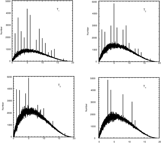
Figure 32: The histogram of pair separations (in comoving proper distances) in the galaxy distribution, for a computer generated toroidal Einstein–de Sitter universe. 50 galaxies are randomly distributed in the cubic fundamental polyhedron, of size 2 500 Mpc. The images are assumed to be visible up to a redshift $z=4$. The peaks reveal the holonomies.

11.8 The distribution of gamma–ray bursts

Gamma–ray bursts were discovered already 20 years ago but their nature and mechanism remain still unknown. In particular we have no idea of their distances and there is presently no consensus about their nature, galactic or extragalactic. Although first observations were consistent with a galactic distribution, the recent results by Meegan et al.  [108] from BATSE (Burst And Transient Source Experiment) suggest a cosmological distribution. However Quashnock & Lamb [129] analyzed the angular distribution of detected bursts and concluded that they appear significantly clustered on angular scales $\approx 4^{\circ}$. From this they suggested that repeated bursts from the same object occured, what would challenge the possible models for cosmological gamma–ray bursts. The burst distribution was later analysed by Narayan & Piran [114] who found also an excess of antipodal pairs. They concluded that both effects were probably due to some selection effects. In this spirit, Maoz [104] proposed an explanation as a “ring bias” due to the satellite localization procedure.

Alternatively, Biesada [13] suggested that these correlated bursts could be due to the multi–connectedness of the Universe, if their sources lie on the principal directions of a small universe. Since the gamma–rays from opposite bursts reach us at approximatively the same time (compared to cosmological time scales), this would imply that the considered bursts all lie at distances $\approx\alpha_{i}/2$, $\alpha_{i}$ being the identification length along a principal direction. This restricts strongly the number of sources which may give rise to such effects. Biesada also correctly remarked that the radiation from a source near a principal direction, and that from its ghost image, should appear as one bright and one faint burst in very close directions. The two corresponding bursts should have been emitted with a time delay $\alpha_{i}/c\approx 10^{9}~{}yrs$. He did not discuss the probability that the same source should experience two bursts separated by a time exactly $\alpha_{i}/c$. Since these correlated bursts would imply a very improbable coincidence, it is unlikely that multi–connectedness is the correct explanation for the angular correlation of bursts.

12 Backgrounds and fields in multi–connected universes

Two different kinds of studies have been made concerning the Cosmic Microwave Background (hereafter CMB) in relation with the possible multi–connectedness of the Universe.

The first is concerned with the homogeneity of the Universe, especially as it appears through the high isotropy of the CMB. Although this homogeneity is a postulated property of the Friedmann–Lemaître models, the question of its origin has been often raised, given that it applies to different parts of the Universe which have never been in causal contact. Tentative answers were considered in the framework of the MCM’s.

The second point of interest concerns the weak angular fluctuations of the CMB, which have now been detected. Such fluctuations are predicted by the current models of galaxy and structure formation, and also by some additional processes. It is thus interesting to ask how the situation is modified in a MCM. Interest toward this question was recently renewed thanks to the last results of the COBE satellite, and recent papers have examined the resulting constraints for the MCM’s.

12.1 An early homogeneization of the Universe

Since homogeneity and isotropy are the funding assumptions of the Friedmann–Lemaître models, it is a logical evidence that they cannot find an explanation in the framework of these models themselves, even if their causal structure has been modified by an early inflationary phase (see §9.3). It is often claimed for instance that the initial conditions of the Friedmann–Lemaître models are “special” or “improbable”. But there is no defined framework in which these words can be given a precise meaning. Quantum cosmology, for instance, which suggests a process distributing the initial conditions, is not presently operative enough to draw firm conclusions.

Concerning inflation, often suggested as a possible explanation for homogeneity, the current models assume that it occurs in a universe whose dynamics is already described by a Friedmann–Lemaître phase, i.e., with initial conditions also “special” : if the pre–inflationary universe was not already sufficiently homogeneous, it has been shown [69] that inflation would not have developed and led to a presently homogeneous universe. In any case, if the CMB homogeneity results from inflation (although no satisfactory candidate has been proposed for the “inflaton”), it only reflects the homogeneity already present in the pre–inflationary universe, at smaller scales.

Thus the causality problem is not solved by inflation and this motivates the search for a causal process which could have homogeneized an initially chaotic (in the sense “highly inhomogeneous”) universe. Rees [131] proposed for instance a model with chaotic initial conditions, in the sense that density fluctuations are always of the order of unity at the scale of the horizon, before the homogeneizing process was active. But this process makes the universe to become more homogeneous with time, over spatial scales comparable to the (ever increasing) horizon  . This process is however “violent”, so that a lot of energy is generated when regions of different densities merge. This energy would be at the origin of the photons which are now present in the Universe. But, in such a model, the process of homogeneization is not expected to have stopped over the cosmic history; in particular, strong anisotropies should have been imprinted over the CMB at the moment of the recombination, so that this model cannot account for its observed isotropy. Rees [131] suggested that a transition from chaotic state to a more uniform situation could have occured at $t\approx t_{eq}$, near the equivalence between the matter and radiation densities, (i.e., before the recombination according to the usual cosmic chronology).

Ellis [35, 36] pointed out that such a model would be compatible with observations if the Universe is multiconnected : a small Universe could have become totally causally connected before the recombination period. Following these first ideas, Gott [72] examined the possibility that the Universe was homogeneized before the recombination  by some causal process : as he stated, “a multi–connected Universe produces the special initial conditions required by the Rees chaotic model.” The solution comes from the fact that the spatial volume of a compact MCM has a finite and “small” value $V$ (and all dimensions are $<\beta$). Thus after a time $\approx\beta/c$, where $c$ is the velocity of light , the whole space is contained within the horizon, i.e., has become causally connected. Therefore a multi–connected universe is and remains completely causally connected from an age $t\approx\beta/c$. For a sufficiently small universe, this occurred before the recombination, so that the CMB isotropy corresponds to the homogeneity of the universe at the recombination, generated by causal effects. Gott [72] and Sokoloff & Shvartsman [142] discussed in more details this possibility.

Gott examined first the simple case of a torus $T^{3}$ ($\Omega=1$). The 3 lengths $\alpha_{x}$, $\alpha_{y}$, and $\alpha_{z}$ are of the same order $\alpha$, to allow a sharp transition between chaotic and smooth Universe [131]. The requirement that the transition occurs near $t_{eq}$ imposes $\alpha/1.15\approx\beta/2\approx R_{horizon}(t_{eq})$, the horizon radius at this period. In the case where the FP is an hexagonal prism, the sharp transition condition suggests a side of the hexagon $\approx 1/\sqrt{3}$ the height of the prism, with $\alpha/1.31\approx\beta/2\approx R_{horizon}(t_{eq})$. He applied the limits on $\alpha$ derived from observations of clusters or superclusters (§11.4). The conclusion was that, for a toroidal space, thermalization of the CMB is marginally excluded by observations, but also marginally admissible. He also stated that, in other types of MCM (with non–flat space), the geometrical constraints and the value of $R_{0}$ imposed by observations do not allow for thermalization. Sokoloff & Shvartsman [142]  also examined the question : with the constraint $\beta\geq 600~{}h^{-1}~{}\mbox{Mpc}$, they estimated that a Friedmann–Lemaître model (without inflation) can only have been homogeneized at a redshift $z\approx$ 10–100 (note that this redshift varies like $1/\beta$), later than the recombination.

Hayward & Twamley [83] adressed the same question in the framework of the MCM’s with negative spatial curvature having the minimum spatial volume (see §10.6.4). They considered a model based on the Weeks–Matveev–Fomenko manifold with a volume $V_{WMF}=0.94~{}R_{0}^{3}$ and a maximum value $L_{max}$ for $\alpha$ given by eq. (50). They considered also a model based on an hypothetic manifold of volume $V_{Meyerhoff}=0.00082~{}R_{0}^{3}$ and $L_{max}$ given by eq. (51). They stated that homogeneization could have been efficient at the recombination if $V<V_{rec}$, the volume of a causally connected region at the recombination. They conclude that a model based on the Meyerhoff arguments may do the job if $\Omega<0.54$, although the one based on the Weeks–Matveev–Fomenko manifold requires $\Omega<0.011$, out of the permitted range.

These conclusions are based on the hypothesis of a standard recombination at $z_{rec}\approx 1\,400$. They would not remain valid if the cosmic matter had suffered a late reionization. In such a case, the Cosmic Microwave Background would originate from, or would have been modified at an epoch much later than $z_{rec}$. This was emphasized by Hayward & Twamley who concluded optimistically, but without really convincing argument, that isotropy of the CMB could be explained in the framework of their models. On the other hand, Gott remarked that the late thermalization of the CMB photons, required in this case, is difficult to include in the model. He thus concluded that this is marginally possible only if $\Omega>1$.

Thus, although multi–connectedness indeed modifies the causal structure of the Universe, calculations show that it is unlikely to explain the spatial homogeneity. This latter must therefore be either admitted as an observed fact without explanation, or accounted for by quantum effects in the early Universe.

12.2 The temperature anisotropies of the CMB

12.2.1 Temperature fluctuations

The search for anisotropies in the CMB is an old story. The dipole anisotropy, detected in 1977, is now well interpreted as the Doppler shift due to the motion of the Earth with respect to the last scattering surface. Its existence, magnitude, and interpretation remain exactly identical in a MCM. Beside the dipole, anisotropy has been detected by the DMR instrument on the COBE satellite, at a very low level $\frac{\Delta T}{T}\approx 10^{-5}$, and at large angular scales $\theta\geq 7^{\circ}$ [139]. In particular the quadrupole component, corresponding to an angle $\theta=90^{\circ}$, appears very low. It is generally admitted that this anisotropy is already present at the recombination epoch. Its level and characteristics may be compared to the predictions of the cosmogonic models, the prototype beeing the cold dark matter model (hereafter cdm). In this frame, an anisotropy at a given angular scale $\theta$ is related to a fluctuation of a spatial scale $L=\frac{\theta}{0.95^{\circ}}~{}100~{}h^{-1}~{}\mbox{Mpc}$ at the recombination time. This relation remains valid, in the universal covering, for a multi–connected universe, since it concerns observational quantities. But, in this case, $L$ may be greater than the dimensions of (real) space, so that no physical fluctuation exists at this scale. Various papers have explored the consequences of this situation.

A tentative detection of the quadrupole anisotropy in the CMB radiation was announced in 1981 [42] and Fagundes [45] suggested that it could be due to multi–connectedness. He estimated the expected effect in the framework of his “quasi–hyperbolic” model (§10.6.3). The latter presents a fundamental anisotropy, described by a parameter $\varepsilon$, which induces a quadrupole component on the CMB :

$$Q=2.7~{}\frac{\varepsilon}{4}~{}\mbox{K}.$$ (52)

Fitting the claimed observational result, he obtained $\varepsilon\approx 1.3~{}10^{-3}$, from what he predicted an anisotropy in the cosmic expansion, unfortunately too weak to be detected. The quadrupole result of 1981 [42] has now been rejected but it remains that multi–connected models may break the symmetry of space, with interesting consequences for the CMB.

In particular, multi–connectedness modifies the relation between angular anisotropies of the CMB and the spatial fluctuations present at the recombination. This is especially the case for values of the topological scale $\alpha$ smaller than the horizon length at the recombination. The last scattering surface is a spherical surface of radius $\approx L_{h}$ (the present horizon length), centered on the observer, in the universal covering. Observing directions separated by an angle $\theta$ is equivalent to observe a comoving length $L=\frac{\theta}{0.95^{\circ}}~{}100~{}h^{-1}~{}\mbox{Mpc}$ on this surface (thus in the universal covering). In a MCM, large values of $\theta$ may correspond to values of $L$ comparable to, or greater than $\alpha$.

The temperature fluctuations $\frac{\Delta T}{T}$ of the CMB are interpreted as the effect of inhomogeneities at the recombination time. They are usually developed into spherical harmonics through the formula

$$\frac{\Delta T}{T}({\bf\hat{q}})=\sum_{l=2}^{\infty}~{}\sum_{m=-1}^{m=l}~{}a_{lm}~{}Y_{l}^{m}({\bf\hat{q}}),$$ (53)

where the coefficients $a_{l}^{m}=\int_{4\pi}~{}d\Omega~{}\frac{\Delta T}{T}({\bf\hat{q}})~{}Y_{l}^{m}({\bf\hat{q}})$ characterise the intensity associated to the harmonic $Y_{l}^{m}({\bf\hat{q}})$. The vector ${\bf\hat{q}}$ denotes a given line of sight on the sky. Homogeneity of space implies a global isotropy of the CMB, so that the moments are rotation–invariant. It is thus sufficient to consider the terms

$$a_{l}^{2}=<\mid a_{l}^{m}\mid^{2}>=\frac{1}{2l+1}\sum_{m=-l}^{l}~{}|a_{l}^{m}|^{2},$$ (54)

defining the angular power spectrum (the two first components define the dipole and quadrupole).

12.2.2 Density perturbations

According to the widely admitted gravitational instability scenario, galaxies and other cosmic structures result from the collapse of initially small density fluctuations. These fluctuations may be treated as small perturbations superimposed onto the strictly homogeneous Friedmann–Lemaître models. They are generally expressed by their expansion into eigenfunctions of the 3–dimensional covariant Laplace operator, usually in Fourier modes. In some respect, a MCM is equivalent to a SCM with additional periodic boundary conditions. As a result, some modes in the expansion are suppressed, those which do not satisfy these conditions. Sokoloff and Starobinski [143] considered these missing modes and defined “G–domains” as the resulting singularities in the distributions of galaxies or clusters, appearing as dark and light spots or bands in the sky. It is important to emphasize that such features are completely different from the ghosts previously discussed. In the present case, a special pattern resulting from the multi–connectedness would be present inside the fundamental polyhedron, and thus be in principle recognizable even in the case where no ghost is observable. The authors concluded, optimistically, that such features could be detected, or their absence demonstrated. But their result strongly depends on their particular model, with a complicated geometry. These effects deserve to be explored in more details, because they offer the possibility of observable consequences even if the multi–connectedness scale is of the order of the present horizon.

12.2.3 Origin of temperature anisotropies

Temperature anisotropies of the CMB may be of two kinds. “Secondary” anisotropies are imprinted on the CMB later than the recombination. We will not consider them here, with the idea that multi–connectedness does not modify their characteristics. On the other hand, “intrinsic” anisotropies are imprinted by the fluctuations in the matter density at the recombination. Although three types of effects (due to the fluctuations in density, velocities and potential) simultaneously contribute, only the fluctuations in the gravitational potential $\delta\phi$ (Sachs–Wolfe effect) matter at angular scales beyond $\ 1^{\circ}$, leading to temperature anisotropies

$$\frac{\Delta T}{T}\approx\delta\phi/3.$$ (55)

Following the gravitational instability scenario, the fluctuations $\delta\phi$ of the gravitational potential are related to those $\delta\rho$ of the mass density through the Poisson equation. Thus, finally, the statistics of $\frac{\Delta T}{T}$ derives from that of $\delta\rho$, or from the density contrast $\delta=\frac{\delta\rho}{<\rho>}$.

Usually, the statistical properties of the scalar field $\delta({\bf x})$ (in real space) are expressed through its spatial Fourier modes $\delta_{k}$. In the idealized case of a gaussian statistics, the power spectrum $P(k)=<\delta_{k}^{2}>$ contains all the information concerning the statistics. Given a model for large scale structure formation, the coefficients $a_{l}^{2}$ may be estimated from the predicted power spectrum $P(k)$. Most models predict, at least at the scales under concern, a power law spectrum $P(k)=<\mid\delta_{k}\mid^{2}>\propto k^{n}$ (that we assume now in the spatial range under study). This corresponds to rms average density and mass contrasts, at the scale $L$

$$<\mid\delta\mid^{2}>^{1/2}\propto\mid\frac{\delta M}{M}\mid^{2}>^{1/2}\propto L^{-\frac{3+n}{2}},$$

and to an average potential fluctuation $<\mid\delta\phi\mid^{2}>^{1/2}\propto L^{\frac{1-n}{2}}$. The corresponding power spectrum for the Fourier transform of the potential is $<\mid\phi_{k}\mid^{2}>\propto k^{n-4}$. The formula (55) allows us to relate the modes $a_{l}^{2}$ to the index $n$. The classical formula reduces to

$$<a_{l}^{2}>=16~{}\pi\sum_{k}\frac{\mid\delta_{k}\mid^{2}~{}j_{l}^{2}(ky)}{(ky)^{4}},$$ (56)

where $j_{l}$ is the $l^{\mbox{th}}$ order spherical Bessel function, and $y$ is the radius of the last scattering surface, well approximated by the present horizon scale (see §10.3.2). The summation extends over all the Fourier modes denoted by ${\bf k}$. Multi–connectedness would limit the possible modes.

12.3 Influence of multi–connectedness

Stevens et al.  [148] and Starobinskii [145] have evaluated this effect, and compared it to the results of the COBE satellite. In a SCM, the sum, extending over all values of $k$, may be estimated through an integral and leads to the classical result

$$<a_{l}^{2}>=<a_{2}^{2}>\frac{\Gamma[(2\ell+n-1)/2]}{\Gamma[(2\ell+5-n)/2]}\frac{\Gamma[(9-n)/2]}{\Gamma[(3+n)/2]},$$ (57)

where $n$ is the slope of the power–law spectrum, and $\Gamma$ the gamma function. For instance, the Harrison–Zeldovich value $n=1$ (relevant for the cdm models) leads to

$$<a_{l}^{2}>\propto\frac{1}{l(l+1)}.$$

However multi–connectedness modifies the situation. When space is compact and finite, at least in some directions, only a restricted collection of wavevectors ${\bf k}$ are allowed. In the case of a torus with sides $\alpha_{x},\alpha_{y},\alpha_{z}$, for instance, the allowed vectors have components $k_{x}=\frac{2\pi n_{x}}{\alpha_{x}},k_{y}=\frac{2\pi n_{y}}{\alpha_{y}}$, and $k_{z}=\frac{2\pi n_{z}}{\alpha_{z}}$, where $n_{x},n_{y},n_{z}$ takes entire values. The sum in (57) is thus restricted to these discrete values. This modifies the spectrum of temperature anisotropies in two respects. First the ratio of the temperature fluctuations level at large angular scales over that at smaller scales is decreased, because there is no direct source (fluctuations of gravitational potential) at the larger scales. Second, the dependence on $\theta$ around the large scales is also modified. Both effects have been considered.

Stevens et al.  [148] considered the simplest case $\alpha_{x}=\alpha_{y}=\alpha_{z}=\alpha$. An Harrison–Zeldovich spectrum of fluctuations ($n=1$) is assumed, as suggested by scale invariance arguments, like those resulting from the idea of inflation (in a MCM, inflation could occur in the same conditions than in a SCM). This spectrum is normalized with the value observed by COBE at the angular scale $\theta=18^{\circ}$. From this fluctuation spectrum, they estimated the statistics of the temperature anisotropies as a function of $\alpha$. Their result includes the values $\alpha=$500, 2 700, 33 000, and 70 000 $h^{-1}~{}\mbox{Mpc}$ , corresponding respectively to 0.15, 0.8, 1 and 20 times the horizon length at recombination. They concluded that the COBE observations could fit their MCM only for $\alpha>2~{}400~{}h^{-1}~{}\mbox{Mpc}$, compared to an horizon size of 3 000 $h^{-1}~{}\mbox{Mpc}$ for their model. For other MCM’s with also zero spatial curvature, a cubic fundamental polyhedron with identifications after 1 or 3 rotations of 180^∘, they obtained limits of 1 600 and $2~{}900~{}h^{-1}~{}\mbox{Mpc}$ respectively.

Starobinskii [145] remarked that, for any MCM with dimension much smaller than the horizon, the power at large angular scale becomes much weaker than the values observed by COBE. Moreover the dependence on $\theta$ must be such that $a_{l}^{2}$ remains almost constant, independent of $l$. This is in contrast to the dependance $a_{l}^{2}\propto\frac{1}{l(l+1)}$ predicted by the $n=1$ spectrum and in accordance with the COBE observations. More precisely he estimated the expected fluctuations to follow

$$a_{l}^{2}=\frac{2\pi}{9}\sum_{k}<\delta\Phi^{2}>~{}(\frac{1}{kL_{rec}})^{2},$$ (58)

where both $k$ and $L_{rec}$, the length of horizon at the recombination, are in comoving units. From this he concluded, with the same reasoning than Stevens et al. , that COBE results exclude a very small Universe. For an identification length much smaller than the present horizon length, this result is independent of the peculiar topology, and of the slope of the power spectrum. This is due to the fact that the fluctuations at large angular scales are created as some “queue–effect” of the spatial fluctuations at much smaller scales (the only existing). In this case, the constancy of $a_{l}$ for large $l$ does not depend on what happens at much smaller scales.

Starobinskii defined another criterion to compare MCM’s with the Cosmic Microwave Background observations. He defined the mode $l_{m}$ as that having the largest multipole amplitude $(\frac{\Delta T}{T})_{l}=\sqrt{\frac{2l+1}{4\pi}}~{}a_{l}$. COBE results imply $l_{m}\leq 6$. Applying this constraint to toroidal universes with three different identification lengths he concluded that the smallest of these values, $\alpha$, must be larger than $0.75L_{h}\approx 9~{}000~{}$Mpc.

Starobinskii also considered cylindrical models, with only one or two compact dimensions. In these two cases, he concluded that the identification lengths (1 or 2) must also obey the previous constraint. But he also remarked that some symmetry (planar or axial, respectively) must be present in the CMB fluctuations. Further observations with improved precision may be able to exclude (or recognize) such symmetries and thus to improve the constraints on MCM’s.

Both papers consider the case of toroidal topology (including the degenerate cases where only 1 or 2 identification lengths are present). Their result rely onto the following hypotheses :

• the Universe is spatially flat with $\Omega=1$.

• there is no strong reionisation after recombination with a high optical depth, so that the Cosmic Microwave Background originates from $z_{recombination}\approx 1400$.

• the COBE anisotropies are intrinsic and due to the Sachs–Wolfe effect only, with a negligible variance.

• the density fluctuations at recombination have a gaussian statistics.

• Starobinskii makes no hypothesis concerning the shape of the fluctuations spectrum. Stevens et al.  study similar cases with the additional hypothesis of a $n=1$ power law spectrum.

Both papers offer convincing evidence that, given the adopted hypotheses, COBE data exclude MCM’s with $\alpha>0.75-0.8~{}L_{h}\approx 2~{}300-2~{}400~{}h^{-1}~{}\mbox{Mpc}$ (the given values are with $h=.5$). Thus, with these hypotheses, the only possible MCMs (for $\Omega=1$) have very large identification lengths and do not offer a great interest from an observational point of view. If one or two identification lengths are infinite, interesting possiblities arise which, following Starobinskii, may lead to peculiar symmetries recognizable in the CMB maps.

The evidence for a $\Omega=1$ Universe is presently not very strong. Although similar qualitative conclusions can be expected if $\Omega<1$, the precise constraints probably differ because of the different geometry of the universal covering, and of the different nature of the holonomies. The calculations remain to be done and it is not certain that the CMB observations bring tighter contraints than those imposed by the geometry itself. Moreover, if one is ready to envisage a multi–connected universe, the question of the formation of large scale structures, as well as the details of the cosmic history should be addressed in a new fashion; the interpretation of the origin and characteristics of the CMB might differ, and the observational constraints derived above would not necessarily hold. In our opinion, this maintains alive the hypothesis of a multi–connected universe with identification lengths smaller than horizon. In particular it seems still justified to search for more direct constraints derived from the apparent distribution of discrete objects at large scale.

12.4 Cosmic magnetic fields

Sokoloff [143] and collaborators [135] examined the relation between possible cosmic magnetic fields and multi–connectedness of space. The presence of large scale intergalactic magnetic fields is suggested by the observed Faraday rotation of distant extragalactic sources (for a more recent review on extragalactic fields, see [93]).

Effects due to multi–connectedness are expected if there exists a magnetic field of constant magnitude and direction over a very large cosmic scale $\lambda$. The strength, which may be $\approx 10^{-9}$ G, plays no role in the study, only the direction and the coherence scale are important. The main idea is that, since both multi–connectedness and a cosmic magnetic field break the isotropy of space, some properties of the anisotropies introduced should coincide.

Sokoloff and collaborators worked in the context of the barrel model, defined in §10.6.5, which provides a good local approximation of a MCM with negative spatial curvature. The case $a=0$, corresponding to a cylindrical universe (thus with flat space), is examined in [135], the case $a\neq 0$ in [143]. The authors suggested to identify the homogeneity scale $\lambda$ of the magnetic field and the identification scale $h$ of the barrel model. Also, they suggested that the principal directions (the axis) of the barrel model may coincide with the direction of the magnetic field; in their view, multi–connectedness and cosmic magnetic fields could have related origins in the early universe, what would explain their coinciding properties. In such a case, the observed direction of a cosmic magnetic field would unveil the principal direction for multi–connectedness, and thus be a precious guide for a search for ghosts. The present observations of extragalactic magnetic fields have however not provided such indice yet.

13 Conclusion

The hypothesis of a multi–connected space widens considerably the variety of universe models obeying the cosmological principle. Although most characteristics of the usual Friedmann–Lemaître solutions are preserved, new and original effects appear. Interesting consequences fall into two categories. First, for an identification length smaller than the horizon, direct observable effects are to be expected onto the appearance of the extragalactic universe. Second, the theoretical interest remains fundamental even if the identification length is comparable or greater than the horizon, in view of the fact that the topology has an important influence on the states of quantum fields.

Directly observable effects may be expected only if the identification length is reachable by present observations. We have reviewed the present observational constraints. The first one, obtained from the distribution of clusters or superclusters, limits $\alpha$ – the shortest circumference of the universe – to a few 10 $h^{-1}~{}\mbox{Mpc}$ and $\beta$ – the maximum dimension inscriptible in real space – to a few 100 $h^{-1}~{}\mbox{Mpc}$. These limits leave room for many observable effects in the distribution of galaxies, clusters, superclusters, quasars, etc. No convincing result has been obtained today from the quasar distribution, and no “exotic effect” is convincingly explained by this hypothesis. Other limits, obtained from the Cosmic Microwave Background observations, are more stringent, since their scales are comparable to that of the horizon, forbidding therefore any directly observable effects. However, given the hypothesis on which it relies, there is some hope that it can be overpassed. For the future, the only observational test which can firmly establish a non–trivial topology is the statistical analysis of reciprocal distances between celestial objects in the universal covering space.

In any case, none of the observational constraints limit the play of multi-connectedness in the early universe. On one hand, the perturbations which have led to the formation of galaxies and large cosmic structures are thought to originate from primordial quantum fluctuations. On the other hand, the fundamental states of the fields themselves play an important role in cosmology. The most famous example is inflation, but other processes only marginally explored up to now, like the Casimir effect, may also influence the cosmic dynamics. In all these aspects, a non–trivial topology would have major consequences. The conclusions from the (still tentative) quantum cosmology are even stronger : they favour a multi–connected rather than a simply–connected universe. Thus, at least from a theoretical point of view, the field of cosmic topology appears not closed but, on the contrary, in a promising state of development.

Acknowledgements

We benefited from discussions with R. Hakim. We deeply thank D. Sokoloff for his numerous suggestions and references, and the referee for his comments. Part of this review is a continuation of the DEA project completed by Miss M.–A. Treyer at the University of Paris VII.

References

- [1] Apanasov, B.N. 1987, Siberian Math. J. 27, 473.
- [2] Arp, H. & Hazard, C. 1980, Ap. J., 240, 726
- [3] Artykbaev, A. & Sokoloff, D. 1991, Geometry as a whole in a flat spacetime, FAN, Tashkent (in Russian)
- [4] Ashtekar, A. & Samuel, J. 1991, Class. Quantum Grav., 8, 2191
- [5] Atiyah, M. 1988, Q.Jl.R.astr.Soc., 29, 287
- [6] Atkatz, D. & Pagels, H. 1982, Phys.Rev.D. 25, 2065
- [7] Beardon, A.F. 1983, The Geometry of Discrete Groups (GTM91) New York:Springer
- [8] Belinskii, V.A., Khalatnikov, I.M. & Lifshitz, E.M. 1970, Advances in Physics 19, 525
- [9] Benedetti, R. & Petronio, C. 1991, Lectures on Hyperbolic Geometry, Springer-Verlag
- [10] Bernshtein, I. N. & Shvartsman, V. F. 1980, Sov. Phys. JETP 52, 814
- [11] Best, L.A. 1971, Canadian J. Math. 23, 451
- [12] Bianchi, L. 1897, Mem.Soc.It.Della. Sc. (Dei.XL) 11 ,267
- [13] Biesada, M. 1993, preprint
- [14] Boothby, M. 1975, An Introduction to Differentiable Manifolds and Riemannian Geometry, Academic, New York, 1975
- [15] Broadhurst, T.J., Ellis, R.S., Koo, D.C. & Szalay, A.S. 1990, Nature, 343, 726
- [16] Burbidge, G.R. 1968, Ap. J., 154, 241
- [17] Burbidge, G.R. 1981, in Proc. of the 10thTexas Symposium on Relativistic Astrophysics, ed. R. Ramaty and F. C. Jones (Ann.NY Acad. Sci. 375 123)
- [18] Burbidge, G.R., Junkkarinen, V. T., Kosli, A.T., Smith, H.E. & Hoag, A.A. 1980, Ap. J., 242, L55
- [19] Bytsenko, A.A. & Goncharov, Y.P. 1991, Class. Quantum Grav. 8, 2269
- [20] Casimir, H. B. G. 1948, Proc. Kon. Ned. Akad. Wet. 51, 793
- [21] Choquet-Bruhat, Y. 1962 in Gravitation : an Introduction to Current Research, ed. L.Witten, Wiley : New York.
- [22] Christenson, J.H., Cronin, J.W., Fitch, V.L. & Turley, R. 1964 Phys.Rev.Lett. 13, 138.
- [23] Chu, Y. & Zhu, X., 1987, A&A, 222, 1
- [24] Coxeter, H., Emmer, M., Penrose, R. & Teuber, M. (eds) 1986, M.C.Escher : Art and Science, Elsevier Science Publishers
- [25] de Sitter, W. 1917a, MNRAS, 78, 3 (also 1916, 76, p. 49; 77, p. 155)
- [26] de Sitter, W. 1917b, Proceedings of the Royal Academy of Amsterdam, 20, 229
- [27] Demianski M. & Lapucha, M. 1987,MNRAS, 224, 527-536
- [28] Deser S., Jackiw R. & ’tHooft G. 1984, Ann. Phys., 152, 220
- [29] Deutsch, D. 1991, Phys. Rev. D, 44, 397
- [30] Eddington, A.S. 1923, The mathematical theory of relativity, CUP., chap. 5
- [31] Efimov, N.V. 1980, Higher Geometry, English transl. P.C. Sinha, Moscow : Mir Publishers
- [32] Einstein, A. 1917, Sitzungsber., Berlin, Febr. 8, p.142
- [33] Eisenhart, L.P. 1926, Riemannnian Geometry, Princeton University Press.
- [34] Elizalde, E. & Kirsten, K. 1993, J.Math.Phys, 35, 3
- [35] Ellis, G.F.R. 1971, Gen.Rel.Grav. 2, 7
- [36] Ellis, G.F.R. 1979, Gen. Rel. Grav. 11, 281
- [37] Ellis, G.F.R. & King, A.R. 1974, Commun.Math.Phys. 38, 114
- [38] Ellis, G.F.R.& McCallum, M.A.H. 1969, Commun.Math.Phys. 12, 108.
- [39] Ellis, G.F.R. 1987, in Theory and observational limits in cosmology, ed. W. R. Stoeger, Specola Vaticana
- [40] Ellis, G.F.R. & Schreiber G. 1986, Phys.Lett.A 115, 97-107
- [41] Estabrook, F.B. Wahlquist, H.D. & Behr, C.G. 1968, J.Math.Phys. 9, 497.
- [42] Fabbri, R. & Melchiorri, F. 1981, Gen.Rel.Grav. 13, 201
- [43] Fagundes, H.V. 1982, Lett. Math.Phys. 6, 417
- [44] Fagundes, H.V. 1983a, Phys. Rev. Lett. 51, 517
- [45] Fagundes, H.V. 1983b, Ap. J., 23, 161
- [46] Fagundes, H.V. 1985, Ap. J., 291, 450
- [47] Fagundes, H. 1985b, Phys.Rev.Lett,. 54, 1200
- [48] Fagundes, H.V. 1986, in Proc. of the Fourth Marcel Grossmann meeting on General Relativity, ed. R. Ruffini, Elsevier (Amsterdam), pp. 1559 – 1563
- [49] Fagundes, H.V. 1989, Ap. J., 338, 618
- [50] Fagundes, H.V. 1992, Gen. Rel. Grav., 24, 199
- [51] Fagundes, H.V. 1993 Phys. Rev. Lett., 70, 1579
- [52] Fagundes, H.V. & Wichoski, U. F. 1987, Ap. J., 322, L57
- [53] Fang, L.–Z. 1990, A&A, 239, 24-28
- [54] Fang, L.–Z., Chu, Y., Liu, Y., & Cao, Ch. 1982, A&A, 106, 287
- [55] Fang, L.–Z. & Mo, H.J. 1987, in Observational Cosmology, eds A. Hewitt, G. Burbidge, L.–Z. Fang, Reidel, Dordrecht, pp.461-475
- [56] Fang, L.–Z. & Sato, H. 1983, Acta Astron Sinica, 24, 410 (also Comm. Theoretical Phys. (China), 2, 1055)
- [57] Fang, L-Z & Sato, H. 1985, Gen.Rel.Grav. 17, 1117
- [58] Fedorov, E. 1885, Russ.J.Crystall.Miner. vol 21
- [59] Fetisova, T., Kuznetsov, D., Lipovetskii, V., Starobinskii, A. & Olovin, R., 1993, Astron.Lett. 19(3), 198
- [60] Fischer, A.E. & Marsden, J.E. 1979 in General Relativity : An Einstein Centenary Survey, Cambridge University Press
- [61] Friedmann, A. 1922, Zeitschr. fur Phys. 10, 377
- [62] Friedmann, A. 1924, Zeitschr. fur Phys. 21, 326
- [63] Fujii, M. 1990, Tokyo J.Math. 13, 353
- [64] Fujiwara, Y. 1993, Class. Quantum Grav. 10, 219
- [65] Geroch, R.P. 1967, J.Math.Phys. 8, 782
- [66] Geroch, R. & Horowitz, G. 1979 in General Relativity : An Einstein Centenary Survey, Cambridge University Press
- [67] Gibbons, G.W. & Hartle, J. B. 1990, Phys. Rev. D, 42, 2458
- [68] Giddings S., Abbot J. & Kuchar K. 1984, Gen. Rel. Grav., 16, 751
- [69] Goldwirth, D.S. & Piran, T. 1992, in The 6th Marcel Grossmann meeting on general relativity, Sato & Nakamura ed., World Scientific, p. 1211
- [70] Goncharov, Y.P. & Bytsenko, A.A. 1989, Astrophys. 27, 422
- [71] Goncharov, Y.P. & Bytsenko, A.A. 1991 Class. Quantum Grav., 8, L211
- [72] Gott, J. R. 1980, MNRAS, 193, 153
- [73] Gott J. R. 1991, Phys. Rev. Lett., 66, 1126
- [74] Gott J. R. & Alpert M. 1984, Gen. Rel. Grav., 16, 243
- [75] Gott J. R., Park M.G. & Lee H.M. 1989, Ap. J., 338, 1
- [76] Gowdy, R.H. 1974, Annals of Physics 83, 2031
- [77] Guggenheimer, H.W. 1963, Differential Geometry, Mac Graw Hill, New–York
- [78] Gurzadyan, V.G. & Kocharyan, A. A. 1987, in Proc. of the Fourth Seminar on Quantum Gravity, eds. M.A.Markov, V.A. Berezin, V.P.Frolov, World Scientific
- [79] Gutsul, I.S. 1979, Soviet J.Math. Dokl. 20, 996.
- [80] Hartle, J.B. & Hawking, S.W. 1983, Phys.Rev.D 28, 2960.
- [81] Hawking, S. 1984, Nuclear Phys. B 239, 257
- [82] Hawking, S.W. & Ellis, G.F.R. 1973, The large–scale structure of spacetime, Cambridge University Press.
- [83] Hayward, G. & Twamley, J. 1990, Phys.Lett. A 149, 84
- [84] Heckmann, O. & Schücking, E. 1962, in Gravitation, an introduction to current research, ed. L.Witten, Wiley, New York, p.438. (Also in Handbuch der Physik, vol.53, p. 515, Springer, Berlin 1959)
- [85] Hewit, A. & Burbidge, G. 1981, Ap. J. S, 43, 57, see also Ap. J. S, 46, 113
- [86] Hilbert, D. & Cohn-Vossen, 1952, Geometry and the Imagination, Chelsea
- [87] Horowitz, G.T. 1991 Class. Quantum Grav., 8, 587
- [88] Kantowski, R. & Sachs, R.K. 1966, J.Math.Phys. 7, 443
- [89] Kardashev, N. 1967, Ap. J. Letters, 150, L135
- [90] Kasner E. 1921, Am.J.Math. 43, 217.
- [91] Kobayashi, S. & Nomizu, K. 1963, Foundations of Differential Geometry (Interscience Pub.: New York).
- [92] Kojima, S. & Miyamoto, Y. 1991, J.Diff. Geom. 34 , 175
- [93] Kronberg, P. P. 1994, Reports on Progress Physics, in press
- [94] Lehoucq, R., Luminet, J.–P. & Lachièze–Rey, M. 1994, preprint
- [95] Lemaître, G. 1929, Rev. Quest. Sci. pp. 189–216 (also first chapter of the book L’hypothè se de l’atome primitif, ed. du Griffon, Neuchatel 1946)
- [96] Lemaître, G. 1931, Rev. Quest. Sci. pp. 391–410 and MNRAS, 91, 490
- [97] Lemaître, G. 1958, in La Structure et l’Evolution de l’Univers, Onziè me Conseil de Physique Solvay. R. Stoops, ed. Brussels : Stoops, pp.1-25
- [98] Löbell, F. 1931, Ber. Sächs.Akad.Wiss.Leipzig 83, 167
- [99] Luminet, J.–P., 1992, Black Holes, Cambridge University Press: Cambridge.
- [100] MacCallum, M.A.H. 1971, Commun. Math. Phys. 20, 57.
- [101] MacCallum, M.A. 1979, in General Relativity : An Einstein Centenary Survey, edited by S.W.Hawking & W.Israel, Cambridge University Press, Chap.11
- [102] MacVittie, G.C. 1956, General Relativity and Cosmology, Chapman and Hall : London
- [103] Magnus, W. 1974, Noneuclidean tesselations and their groups (New York:Academic).
- [104] Maoz, E. 1993, preprint astro-ph/9308040
- [105] Maskit, B. 1971, Adv. in Math. 7, 219
- [106] Massey, W.S. 1987, Algebraic Topology : an introduction, Springer–Verlag
- [107] Matveev, S.V. & Fomenko, A.T. 1988, Russian Math. Surveys 43, 3
- [108] Meegan, C. et al. 1992, Nature, 355, 143
- [109] Meyerhoff, R. 1986, Commun. Math.Helv. 61, 271
- [110] Misner, C.W. 1969b, Phys.Rev. Lett. 22, 1071.
- [111] Misner, C.W. 1972, in Klauder J. (Ed.) Magic without Magic (Freeman, San Francisco).
- [112] Morris M. S., Thorne K. S., & Yurtsever U. 1988, Phys. Rev. Lett., 61, 1446
- [113] Mostow, G.D. 1973, Ann. Math. Studies 78, Princeton University Press, Princeton, New Jersey.
- [114] Narayan, R. & Piran, T. 1993, preprint astro-ph/9308007
- [115] Narlikar, J.V. & Seshadri, T.R. 1985, Ap.J., 288, 43
- [116] Nash, C. & Sen, S. 1983 Topology and Geometry for Physicists, Academic Press
- [117] Neumann, W.D.& Zagier, D. 1985, Topology 24(3), 307
- [118] Osinovsky, M.E. 1973, Ann. Inst. Henri Poincaré 19, 197
- [119] Paál G. 1971, Acta Phys. Acad. Scient. Hungaricae, 30, 51
- [120] Park, C. & Gott, J.R. 1991, MNRAS, 249, 288
- [121] Penrose, R. 1972, Techniques of Differential Topology in Relativity, Society for Industrial and Applied Mathematics, Philadelphia
- [122] Penrose, R. 1979 in General Relativity : An Einstein Centenary Survey, Cambridge University Press.
- [123] Penrose, R. & Rindler, W. 1984, Spinors and Spacetime, C.U.P.
- [124] Peterson, M.A., 1979, Am.J.Phys. 47, 1031.
- [125] Petrosian, V., Salpeter, E. & Szekeres, P. 1967, Ap. J., 147, 1222
- [126] Petrov, A.Z. 1969, Einstein spaces (Pergamon, Oxford)
- [127] Poincaré, H., 1953, Oeuvres de Henri Poincaré Vol.VI, Gauthier-Villars : Paris
- [128] Prasad, G. 1973, Invent. Math. 21, 255
- [129] Quashnock, J. M. & Lamb, D.Q. 1994, preprint
- [130] Rêgo & Rourke, 1986, cited in I.Stewart, Nature, 320, 217
- [131] Rees, M.J. 1972, Phys. Rev. Lett., 28, 1669
- [132] Rhoades, J.E. & Gott, J. R. 1994, Ap. J., 421, 1
- [133] Ryan, M.P. & Shepley, L.C. 1975 Homogeneous Relativistic Cosmologies, Princeton University Press
- [134] Ryan, M.P. Jr. 1972, Hamiltonian Cosmology, Lecture Notes in Physics, vol. 13, Springer-Verlag: Berlin.
- [135] Ruzmaikin, A. & Sokoloff, D.D. 1977, Astrophysics (Armenia), 13, 95
- [136] Scott, P. 1983, Bull. London Math. Soc. 15, 401
- [137] Seifert, H. & Threlfall, W. 1930, Math.Ann. 104, 1, English transl. M.A. Goldman, New York : Academic
- [138] Seifert, H. & Weber, C. 1933, Math.Z. 37, 237
- [139] Smoot, G. et al. 1992, Ap. J. Letters, 396, L1
- [140] Sokoloff, D.D. 1971, Sov.Phys.Dokl. 15, 1112
- [141] Sokoloff, D.D. 1975, Sov. Astron. Lett., 1, 113
- [142] Sokoloff, D.D. & Shvartsman, V.F. 1974, Sov. Phys. JETP, 39 196
- [143] Sokoloff, D.D. & Starobinskii A.A. 1975, Sov.Astron. 19, 629
- [144] Sokoloff, D. 1977, Gravitation and Relativity, 12, 142 (in Russian).
- [145] Starobinskii, A.A. 1994, preprint
- [146] Staruszkiewicz, A. 1963, Acta Phys. Polonica 24, 734
- [147] Steenrod, N.E. 1951, The topology of fiber bundles, Princeton Univ. Press
- [148] Stevens, D., Scott, D. & Silk, J. 1993, Phys. Rev.Lett. 71, 20
- [149] Streater, R.F. & Wightman, A.S. 1964 PCT, Spin Statistics and All That, Benjamin : New York.
- [150] Thurston, W.P. 1979, The geometry and topology of three manifolds, Princeton Lecture Notes
- [151] Thurston, W.P. 1982, Bull.Am.Math.Soc. 6, 357
- [152] Thurston, W.P. & Weeks, J.R. 1984, Sci.Am. July, p.94
- [153] Triay, R. 1982, The Catalog of High Redshifts, Marseille–University publications
- [154] Weeks, J.R. 1985, PhD thesis, Princeton University
- [155] Weinberg, S. 1972, Gravitation and Cosmology, (Wiley: New York).
- [156] Winstein, B. & Wolfenstein, L. 1993, Rev. Mod. Phys. 65, 1113
- [157] Witten, E. 1988, Nucl.Phys. B 311, 46
- [158] Wolf, J. 1984, Spaces of constant curvature, Fifth Edition, Publish or Perish Inc, Wilmington (USA)
- [159] Wu, C.S. 1957 Phys.Rev. 105 1413.
- [160] Zeldovich, Ya. B. & Novikov, I.D. 1967, JETP letters, 6, 639
- [161] Zeldovich, Ya. B. 1970, A&A, 5, 84
- [162] Zeldovich, Ya B. 1973, Comm.Astrophys.Space Phys.5, 169
- [163] Zeldovich, Ya B. 1982, in Astrophysical Cosmology, Proc.Vatican Study Week on Cosmology and Fundamental Physics, ed. H.A.Brück, G.V.Coyne and M.S.Longair (Rome: Specola Vaticana), p.575
- [164] Zeldovich, Ya.B., Sokoloff, D. & Starobinskii A. 1977, Some problems of geometry as a whole in general relativity, in 150 years of the Lobachevsky geometry. Invited lectures, ed. Institute of Scientific and Technic Information, Moscow, 1977, pp.271-282 (in Russian)
- [165] Zel’dovich, Y.B. & Grishchuk, L.P.1984, MNRAS, 207, 23P