Abstract

A model of a fluctuating lightcone due to a bath of gravitons is further investigated. The flight times of photons between a source and a detector may be either longer or shorter than the light propagation time in the background classical spacetime, and will form a Gaussian distribution centered around the classical flight time. However, a pair of photons emitted in rapid succession will tend to have correlated flight times. We derive and discuss a correlation function which describes this effect. This enables us to understand more fully the operational significance of a fluctuating lightcone. Our results may be combined with observational data on pulsar timing to place some constraints on the quantum state of cosmological gravitons.

1 Introduction

In a previous paper [1], henceforth I, the problem of lightcone fluctuations due to gravitons was discussed. A bath of gravitons in a squeezed vacuum state, or a thermal state, was shown to produce fluctuations of the spacetime metric, which in turn produce lightcone fluctuations. (A squeezed vacuum state is the state in which relict gravitons from the early universe are expected to be found [4].) The propagation time of a classical light pulse [2] over a distance $r$ is no longer precisely $r$ [3], but undergoes fluctuations around a mean value of $r$. In I, it was shown that the mean deviation from the classical propagation time is

$$\Delta t=\frac{\sqrt{\langle\sigma_{1}^{2}\rangle}}{r}\,,$$ (1)

where $\langle\sigma_{1}^{2}\rangle$ is the mean square fluctuation in the geodesic interval function. Let $\sigma(x,x^{\prime})$ be one-half of the squared geodesic distance between a pair of points $x$ and $x^{\prime}$. In the presence of a linearized metric perturbation $h_{\mu\nu}$,

$$\sigma=\sigma_{0}+\sigma_{1}+O(h_{\mu\nu}^{2})\,.$$ (2)

Here $\sigma_{0}=\frac{1}{2}(x-x^{\prime})^{2}$ is the flat space interval function, and $\sigma_{1}$ is the first order shift in $\sigma$, which becomes a quantum operator when the metric perturbations are quantized, The expectation values of $\sigma_{1}^{2}$ are formally divergent, so $\langle\sigma_{1}^{2}\rangle$ is understood to be a renormalized expectation value, the difference between the expectation value in a given state and in the Minkowski vacuum state. Note that we are assuming that the metric fluctuations are produced solely by the bath of gravitons. More generally, quantum matter fields will experience stress tensor fluctuations which will act as an additional source of metric fluctuations [5, 6].

Equation (1) arises from a calculation given in I of the expectation value of the retarded Green’s function in a squeezed vacuum state of gravitons, which yielded

$$\Bigl{\langle}G_{ret}(x,x^{\prime})\Bigr{\rangle}={{\theta(t-t^{\prime})}\over{8\pi^{2}}}\sqrt{\pi\over{2\langle\sigma_{1}^{2}\rangle}}\;\exp\biggl{(}-{{\sigma_{0}^{2}}\over{2\langle\sigma_{1}^{2}\rangle}}\biggr{)}\,.$$ (3)

This form is valid for the case that $\langle\sigma_{1}^{2}\rangle>0$. Equation (3) reveals that the delta-function behavior of the classical Green’s function, $G_{ret}$, has been smeared out into a Gaussian function which is peaked around the classical lightcone. This means that a light pulse is equally likely to traverse a distance in less than the classical propagation time as it is to traverse the interval in a longer time.

In I, explicit forms of $\langle\sigma_{1}^{2}\rangle$ were given for particular quantum states, including a single mode squeezed vacuum state and a thermal state in the long wavelength limit. One of the purposes of the present paper is to generalize these calculations, in particular to a bath of thermal gravitons in the short wavelength limit. This will be done in Sect. 2.

The primary purpose of this paper will be to calculate and interpret the correlation function which relates the flight time variations of a pair of successive photons. In general, such a pair of photons may have correlations which causes the expected difference in their flight times to be less than $\Delta t$. If one wishes to use observational data to search for flight time variations due to lightcone fluctuations, it is essential to understand these correlations. In Sect. 3, a general formula for the correlation function $\Bigl{\langle}G_{ret}(x_{2},x_{1})G_{ret}(x^{\prime}_{2},x^{\prime}_{1})\Bigr{\rangle}-\Bigl{\langle}G_{ret}(x_{2},x_{1})\Bigr{\rangle}\Bigl{\langle}G_{ret}(x^{\prime}_{2},x^{\prime}_{1})\Bigr{\rangle}$ is obtained. In Sect. 4, this function is used to determine when pairs of photons are correlated, and to calculate the mean variation in flight times, $\delta t$. In Sect. 5, we first review the effects of classical gravity waves upon pulse arrival times, and the bounds which pulsar timing data yield upon a background of such classical waves. We then discuss the bounds which this data place upon gravitons in a squeezed vacuum state. Our results are summarized and discussed in Sect. 6.

2 Calculation of $\langle\sigma_{1}^{2}\rangle$ for a Thermal Bath of Gravitons

In I, $\langle\sigma_{1}^{2}\rangle$ was calculated for a thermal bath of gravitons in the low temperature limit. In this section, we wish to generalize this calculation to arbitrary temperature, and in particular obtain the high temperature limit. In the transverse-tracefree gauge, the graviton two-point function is expressible in terms of that for a massless scalar field: [7]

$$\langle h_{ij}(x)h^{ij}(x^{\prime})\rangle=2\langle\varphi(x)\varphi(x^{\prime})\rangle\,.$$ (4)

From this expression, and Eqs. (49) and (61) of I, we obtain

$$\langle\sigma_{1}^{2}\rangle={1\over{15}}\,r^{2}\,\int_{0}^{r}dz\int_{0}^{r}dz^{\prime}\>\,\langle\varphi(x)\varphi(x^{\prime})\rangle\,,$$ (5)

where the integrals are to be evaluated along the unperturbed null geodesic, We take this geodesic to have a spatial extent of $r$ in the $z$ direction, so $x=(z,0,0,z)$ and $x^{\prime}=(z^{\prime},0,0,z^{\prime})$. Using the fact that the two-point function is a function of $\rho=|{\bf x}-{\bf x^{\prime}}|=|z-z^{\prime}|$, we may change variables of integration and write

$$\langle\sigma_{1}^{2}\rangle={2\over{15}}r^{2}\int_{0}^{r}d\rho\,(r-\rho)\>\,\langle\varphi(x)\varphi(x^{\prime})\rangle\,.$$ (6)

Note that the two-point function and the Hadamard function, $G(x,x^{\prime})=\frac{1}{2}\langle\{\varphi(x)\varphi(x^{\prime})\}\rangle$, are related by

$$\langle\varphi(x)\varphi(x^{\prime})\rangle=G(x,x^{\prime})+\frac{i}{2}\Bigl{[}G_{adv}(x,x^{\prime})-G_{ret}(x,x^{\prime})\Bigr{]}\,,$$ (7)

where $G_{adv}(x,x^{\prime})$ and $G_{ret}(x,x^{\prime})$ are the advanced and retarded Green’s functions, respectively. Because the latter are proportional to delta functions of the form $\delta(t-t^{\prime}\pm|{\bf x}-{\bf x}^{\prime}|)$, they will not contribute to the renormalized thermal function, which is expressible as an image sum over imaginary time. Thus for our purposes, the two-point and Hadamard functions are identical. Some of the properties and limits of the renormalized thermal two-point function, which we will denote by $G_{RT}(x,x^{\prime})$, are discussed in the Appendix.

A true thermal bath has both its characteristic wavelength, $\lambda_{g}=\beta$, and its graviton density determined by the temperature, $\beta^{-1}$. We will also be interested in more general baths with an approximately Planckian spectrum but an arbitrary amplitude. The mean squared amplitude of the metric fluctuations is characterized by the quantity

$$h^{2}=\frac{1}{30}\langle h_{ij}(x)h^{ij}(x)\rangle\,.$$ (8)

In the case of a thermal bath

$$h^{2}=\frac{1}{180\,\beta^{2}}\,,$$ (9)

so if we let

$$\langle\varphi(x)\varphi(x^{\prime})\rangle=180\,\beta^{2}\,h^{2}\,G_{RT}(x,x^{\prime})\,,$$ (10)

we obtain the two-point function for a more general bath with a Planckian spectrum. In the following discussion, we will often use the symbols $\beta$ and $\lambda_{g}$ interchangeably. However, in general $\beta$ is understood to be the inverse temperature for a thermal bath, and $\lambda_{g}$ the mean wavelength for a more general bath.

In the short wavelength (high temperature limit), we may use the asymptotic form for the thermal two-point function on the lightcone, Eq. (A12), to write

$$\langle\sigma_{1}^{2}\rangle\approx{3\over\pi}\,r^{2}\,\lambda_{g}h^{2}\,\int_{a\lambda_{g}}^{r}d\rho\,(r-\rho)\>\,\frac{1}{\rho}\,.$$ (11)

Recall that this asymptotic form is valid only for $\rho>a\lambda_{g}$, where $a\gg 1$ is a constant. Thus we have introduced a cutoff at $\rho=a\lambda_{g}$ in the integral. This introduces an error of $O(\lambda_{g}^{0})$, which is small in the $\lambda_{g}\rightarrow 0$ limit. Evaluation of the integral in Eq. (11) yields

$$\langle\sigma_{1}^{2}\rangle\approx{3\over\pi}\,h^{2}\,r^{3}\,\lambda_{g}\,\biggl{[}\ln\biggl{(}\frac{r}{\lambda_{g}}\biggl{)}+c_{1}\biggl{]}\,.$$ (12)

where $c_{1}$ is a constant of order unity.

In I, the corresponding expression was derived for the low temperature (long wavelength) limit, where it was shown that

$$\langle\sigma_{1}^{2}\rangle\approx h^{2}\,r^{4}\,,$$ (13)

for a general long wavelength graviton bath ($\lambda_{g}\gg r$). Note that comparison of Eqs. (12) and (13) reveals that $\langle\sigma_{1}^{2}\rangle$ always grows with increasing $r$, but somewhat more slowly in the large distance limit where $r>\lambda_{g}$.

3 The Correlation Function

In this section, we wish to derive and interpret an expression for the correlation function

$$C(x_{2},x_{1};x^{\prime}_{2},x^{\prime}_{1})\equiv\Bigl{\langle}G_{ret}(x_{2},x_{1})G_{ret}(x^{\prime}_{2},x^{\prime}_{1})\Bigr{\rangle}-\Bigl{\langle}G_{ret}(x_{2},x_{1})\Bigr{\rangle}\Bigl{\langle}G_{ret}(x^{\prime}_{2},x^{\prime}_{1})\Bigr{\rangle}\,.$$ (14)

Our starting point is the Fourier representation of the retarded Green’s function,

$$G_{ret}(x_{2},x_{1})={{\theta(t_{2}-t_{1})}\over{8\pi^{2}}}\int_{-\infty}^{\infty}d\alpha\,e^{i\alpha\sigma_{0}}\,e^{i\alpha\sigma_{1}}\,.$$ (15)

We may follow a procedure analogous to that used in I to obtain $\Bigl{\langle}G_{ret}(x_{2},x_{1})\Bigr{\rangle}$ to find

$$\Bigl{\langle}G_{ret}(x_{2},x_{1})G_{ret}(x^{\prime}_{2},x^{\prime}_{1})\Bigr{\rangle}=\frac{\theta(t_{2}-t_{1})\theta(t^{\prime}_{2}-t^{\prime}_{1})}{128\pi^{3}\,\sqrt{B}}\,\exp\biggl{(}-\frac{A}{2B}\biggr{)}\,,$$ (16)

where

$$A=\sigma_{0}^{2}\langle{\sigma^{\prime}_{1}}^{2}\rangle+{\sigma^{\prime}_{0}}^{2}\langle\sigma_{1}^{2}\rangle-2\sigma_{0}\sigma^{\prime}_{0}\langle\sigma_{1}\sigma^{\prime}_{1}\rangle\,,$$ (17)

and

$$B=\langle\sigma_{1}^{2}\rangle\langle{\sigma^{\prime}_{1}}^{2}\rangle-\langle\sigma_{1}\sigma^{\prime}_{1}\rangle^{2}\,.$$ (18)

Here $\sigma_{0}$ and $\sigma_{1}$ refer to the pair of points $(x_{2},x_{1})$, whereas $\sigma^{\prime}_{0}$ and $\sigma^{\prime}_{1}$ refer to $(x^{\prime}_{2},x^{\prime}_{1})$. Equation (16) is valid only if $B>0$.

Let us consider the limit in which $\langle\sigma_{1}\sigma^{\prime}_{1}\rangle$ is small, so that

$$A\approx\sigma_{0}^{2}\langle{\sigma^{\prime}_{1}}^{2}\rangle+{\sigma^{\prime}_{0}}^{2}\langle\sigma_{1}^{2}\rangle\,,$$ (19)

and

$$B\approx\langle\sigma_{1}^{2}\rangle\langle{\sigma^{\prime}_{1}}^{2}\rangle\,.$$ (20)

In this limit, $\Bigl{\langle}G_{ret}(x_{2},x_{1})G_{ret}(x^{\prime}_{2},x^{\prime}_{1})\Bigr{\rangle}\approx\Bigl{\langle}G_{ret}(x_{2},x_{1})\Bigr{\rangle}\Bigl{\langle}G_{ret}(x^{\prime}_{2},x^{\prime}_{1})\Bigr{\rangle}$ and hence we have $C(x_{2},x_{1};x^{\prime}_{2},x^{\prime}_{1})\approx 0$. Thus, successive pulses are uncorrelated and the expected variation in their flight times is given by Eq. (1).

More generally, $C(x_{2},x_{1};x^{\prime}_{2},x^{\prime}_{1})\not=0$, and a pair of successive pulses will be correlated. In this case, the expected variation in their flight times is not given by Eq. (1), but is expected to be smaller. Recall that the function $\Bigl{\langle}G_{ret}(x_{2},x_{1})G_{ret}(x^{\prime}_{2},x^{\prime}_{1})\Bigr{\rangle}$ is the mean value of the product of the field at $x_{2}$ due to a delta function source at $x_{1}$ with the field at $x^{\prime}_{2}$ due to a delta function source at $x^{\prime}_{1}$. In the absence of metric fluctuations, this quantity is nonzero only when the propagation times are equal, that is, when $t_{2}-t_{1}=t^{\prime}_{2}-t^{\prime}_{1}$. In the presence of metric fluctuations, this function is a Gaussian peaked at the point where $t_{2}-t_{1}=t^{\prime}_{2}-t^{\prime}_{1}$, and with a width which characterizes the expected deviation in propagation times. This behavior will be illustrated by specific examples in the following section.

4 Variation in Photon Flight Times

In this section, we wish to consider the situation illustrated in Fig. 1, where a photon is emitted at $t=t_{1}$ and detected at $t=t_{2}$ and then a second photon is emitted at $t=t^{\prime}_{1}$ and detected at $t=t^{\prime}_{2}$. Let $t_{0}=t^{\prime}_{1}-t_{1}$, the difference in emission times. The effects of metric fluctuations will in general cause the propagation times, $t_{2}-t_{1}$ and $t^{\prime}_{2}-t^{\prime}_{1}$, to differ both from the classical propagation time, $r$, and from one another. Let $\Delta t$ be the expected deviation from the classical time for either photon:

$$\Delta t=\sqrt{\langle(t_{2}-t_{1}-r)^{2}\rangle}=\sqrt{\langle(t^{\prime}_{2}-t^{\prime}_{1}-r)^{2}\rangle}=\frac{\sqrt{\langle\sigma_{1}^{2}\rangle}}{r}\,.$$ (21)

Let $\delta t$ be the expected variation in the propagation times of successive photons:

$$\delta t^{\prime}=\sqrt{\langle(t_{2}-t_{1}-t^{\prime}_{2}+t^{\prime}_{1})^{2}\rangle}\,.$$ (22)

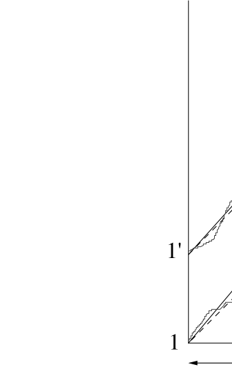
Figure 1:

A photon is emitted at point $1$ and detected at point $2$. A second photon is emitted at point $1^{\prime}$ and detected at point $2^{\prime}$. In the absence of metric fluctuations, a photon propagates on the classical lightcone, illustrated by the dashed lines. Metric fluctuations cause the the photon to move on a stochastic trajectory with a propagation time which may either larger or smaller than the classical flight time. The mean trajectory for a fixed flight time is illustrated by the solid lines.

When the propagation of the two photons is uncorrelated, $\delta t=\Delta t$. We expect this to be the case when the difference in emission times, $t_{0}$, is sufficiently long. More generally, the photons may be correlated, in which case $\delta t<\Delta t$. Various special cases will be discussed in the following subsections. We will need to calculate $\langle\sigma_{1}\sigma^{\prime}_{1}\rangle$, which is given by an expression analogous to Eq. (5) :

$$\langle\sigma_{1}\sigma^{\prime}_{1}\rangle={1\over{15}}\,r^{2}\,\int_{0}^{r}dz\int_{0}^{r}dz^{\prime}\>\,\langle\varphi(x)\varphi(x^{\prime})\rangle\,,$$ (23)

where the $z$-integration is taken along the mean path of the first photon, and the $z^{\prime}$-integration is taken along that of the second photon. Here we will assume that $\Delta t\ll r$, so the slopes, $v$ and $v^{\prime}$, of the two mean paths are approximately unity. Thus the two-point function in Eq. (23) will be assumed to be evaluated at $\rho=|{\bf x}-{\bf x^{\prime}}|=|z-z^{\prime}|$ and $\tau=|t-t^{\prime}|=|z-z^{\prime}-t_{0}|$.

4.1 Large $t_{0}$

Let us first consider the limit in which $t_{0}$ is large compared to either $r$ or $\lambda_{g}$, and hence the integration in Eq. (23) is over points for which $\tau\approx t_{0}\gg\rho$ and $\tau\gg\lambda_{g}$. In this limit, the two-point function becomes approximately [See Eq. (A9).]

$$\langle\varphi(x)\varphi(x^{\prime})\rangle\approx\frac{45\,\lambda_{g}^{2}\,h^{2}}{\pi^{2}\,\tau^{2}}\,.$$ (24)

Thus, we find

$$\langle\sigma_{1}\sigma^{\prime}_{1}\rangle\approx 3\,\lambda_{g}^{2}\,h^{2}\,\frac{(\Delta t)^{4}}{\pi^{2}\,t_{0}^{2}}\,.$$ (25)

In this limit, $\langle\sigma_{1}\sigma^{\prime}_{1}\rangle\ll\langle\sigma_{1}^{2}\rangle$, and we obtain the uncorrelated case. In the long graviton wavelength (low temperature) limit, $\langle\sigma_{1}^{2}\rangle$ is given by Eq. (13) and we have

$$\delta t\approx\Delta t=h\,r\,.$$ (26)

In the short graviton wavelength (high temperature) limit, $\langle\sigma_{1}^{2}\rangle$ is given by Eq. (12) and

$$\delta t\approx\Delta t=h\,\sqrt{\frac{3}{\pi}\,r\,\lambda_{g}}\;\sqrt{\ln\biggl{(}\frac{r}{\beta}\biggr{)}+c_{1}}\,.$$ (27)

4.2 Long Graviton Wavelengths

In the limit in which $\lambda_{g}$ is large compared to both $r$ and to $t_{0}$, we use the low temperature approximation to the thermal two-point function, Eq. (A7). Substituting this approximate form into Eq. (6) yields

$$\langle\sigma_{1}^{2}\rangle\approx h^{2}\,r^{4}\;\biggl{[}1-\frac{2\,\pi^{2}\,r^{2}}{45\,\lambda_{g}^{2}}\biggl{]}\,.$$ (28)

Similarly, we obtain

$$\langle\sigma_{1}\sigma^{\prime}_{1}\rangle\approx\langle\sigma_{1}^{2}\rangle-h^{2}\,\frac{\pi^{2}\,r^{4}\,t_{0}^{2}}{5\,\lambda_{g}^{2}}\,,$$ (29)

and hence combining these two results, we obtain

$$B\approx 2h^{4}\,\frac{\pi^{2}\,r^{8}\,t_{0}^{2}}{5\,\lambda_{g}^{6}}\,.$$ (30)

In the calculation of $B$, it was possible to approximate the slopes of the photon trajectories as being unity. In order to obtain nonvanishing expressions for $\sigma_{0}$ and $\sigma^{\prime}_{0}$, we must consider the deviation of these slopes, $v$ and $v^{\prime}$, from unity. To leading order in $|v-1|$ and $|v^{\prime}-1|$, we have

$$\sigma_{0}^{2} \approx (1-v)^{2}\,r^{4}$$

$${\sigma^{\prime}_{0}}^{2} \approx (1-v^{\prime})^{2}\,r^{4}$$

$$\sigma_{0}\sigma^{\prime}_{0} \approx (1-v)(1-v^{\prime})\,r^{4}\,.$$ (31)

For the calculation of $A$, we use only the approximation in which

$$\langle\sigma_{1}^{2}\rangle\approx\langle{\sigma^{\prime}_{1}}^{2}\rangle\approx\langle\sigma_{1}\sigma^{\prime}_{1}\rangle\approx h^{2}\,r^{4}\,.$$ (32)

Then we obtain

$$A\approx h^{2}\,r^{8}(v-v^{\prime})^{2}\,,$$ (33)

The magnitude of the argument of the exponential in Eq. (16) becomes

$$C=\frac{A}{2B}\approx\frac{5\,\beta^{2}\,(v-v^{\prime})^{2}}{4\,\pi^{2}\,h^{2}\,t_{0}^{2}}\,.$$ (34)

In this case, $\langle\sigma_{1}\sigma^{\prime}_{1}\rangle$ is not negligible, and hence the two photons are correlated. The mean variation in the flight times is given by $\delta t=\delta v\,r$, where $\delta v$ is the value of $|v-v^{\prime}|$ for which $C=1$. Thus

$$\delta t\approx\frac{2\pi}{\sqrt{5}}\biggl{(}\frac{t_{0}}{\lambda_{g}}\biggr{)}h\,r\,.$$ (35)

From Eqs. (1) and (13), we see that

$$\Delta t\approx h\,r\,$$ (36)

and hence that $\delta t\ll\Delta t$, i.e., the photons are highly correlated.

4.3 Large Separations

In this section, we will consider the case where the separation $r$ is larger than either the graviton wavelength $\lambda_{g}$ or the temporal separation between the pulses, $t_{0}$. The integrations in Eq. (23) now involves pairs of points with timelike, spacelike, and null separations, as illustrated in Fig. 2. This is contrast to the situation in Sect. 4.1, where the integrations are entirely over pairs of timelike separated points. We will assume that $r\gg\lambda_{g}$. Thus we may use the high temperature form of the thermal two-point function, which is given by Eq. (A9) for timelike separations, and Eq. (A10) for spacelike separations. Recall that the former form is valid only for $\tau-\rho>\beta=\lambda_{g}$. Thus the timelike separated point points will yield a contribution to $\langle\sigma_{1}\sigma^{\prime}_{1}\rangle$ which is of $O(\ln\lambda_{g})$. However, the spacelike separated points yield a contribution which is of $O(\lambda_{g}^{-1})$, and hence is dominant in the small $\lambda_{g}$ limit. Inserting Eq. (A10) into Eq. (23), and integrating over spacelike separated points yields

$$\langle\sigma_{1}\sigma^{\prime}_{1}\rangle\approx\frac{3}{\pi}\,h^{2}\,\lambda_{g}\,r^{2}\int_{0}^{r}dz\int_{0}^{z-t_{0}}dz^{\prime}\>\,\frac{1}{\rho}\,=\frac{3}{\pi}\,h^{2}\,\lambda_{g}\,r^{3}\;\biggl{[}\,\ln\biggl{(}\frac{r}{t_{0}}\biggl{)}\,-\,1\biggl{]}\,.$$ (37)

Compare this result with Eq. (12) for $\langle\sigma_{1}^{2}\rangle$ in the $r\gg\lambda_{g}$ limit. We see that

$$\frac{\langle\sigma_{1}\sigma^{\prime}_{1}\rangle^{2}}{\langle\sigma_{1}^{2}\rangle\,\langle{\sigma^{\prime}_{1}}^{2}\rangle}\approx\frac{\ln\bigl{(}{r}/{t_{0}}\bigl{)}}{\ln\bigl{(}{r}/{\lambda_{g}}\bigl{)}}\,.$$ (38)

Thus far, we have not specified the relative magnitudes of $\lambda_{g}$ and $t_{0}$. Let first consider the case $\lambda_{g}\ll t_{0}$. In this limit, the ratio in Eq. (38) slowly approaches zero. Thus, in this case, the two photons become uncorrelated. Because of the slow rate at which this ratio vanishes, we might describe this case as one in which the events are weakly uncorrelated, and the variation in the flight times is approximately given by Eq. (27).

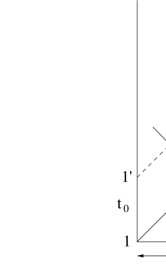
Figure 2:

The domain of integration in Eq. (23) is illustrated for the case that $r>t_{0}$. For a given point $(t,z)$ on the first trajectory, a point $(t^{\prime},z^{\prime})$ on the second trajectory may spacelike separated (dashed line) or timelike separated (solid line) from the first point. The boundary case of null separation occurs at $z^{\prime}=z-t_{0}$. In the high temperature limit, $r\gg\beta$, the spacelike portion yields the dominant contribution to the integral.

The remaining possibility is the case where $\lambda_{g}>t_{0}$. The ratio in Eq. (38) is now larger than unity, and hence $B<0$. In this case, the derivation of the correlation function given in Sect. 3 breaks down, and our results are inconclusive.

5 Effects of Cosmological Gravitons

In principle, the results of the previous sections could be used to search for relict cosmological gravitons. It is expected that there may exist a bath of gravitons at the present time which was created in the early universe. For example, if the universe evolved from a state of thermal equilibrium at the Planck epoch without inflation, one would expect that there should now be a thermal bath of gravitons at a temperature of approximately $3K$. On the other hand, inflation would tend to wipe out such a bath, but could create more gravitons at the end of inflation. Inflation at an energy scale of the order of $10^{15}$ GeV might produce a bath with $\lambda_{g}\approx 10^{4}{\rm cm}$ and $h\approx 10^{-36}$ [1, 8]. The effects of either of these baths upon the propagation time of photons is far too small to be detectable, however.

We can take a different approach in which we conjecture that some unknown process may have generated a much larger bath of gravitons, and seek observational bounds on such a bath. The timing data from pulsars provides one such set of bounds. This data has in fact been used in recent years to place limits on a background of classical gravity waves [9]-[12]. Thus, in the next subsection, we will briefly review the effect of a classical gravity wave upon the observed arrival times of pulses.

5.1 Classical Gravity Waves and Photon Flight Times

Consider a classical metric perturbation, $h_{ij}$, in the transverse-tracefree (TT) gauge. If one photon is emitted at $t=0$ and a second at $t=t_{0}$, the difference in their flight times over a spatial distance $r$ is (See Ref. [9] and Eq. (46) in I.)

$$\Delta\,T=-\frac{1}{2}\int_{0}^{r}[H(t_{0}+z,z)\,-\,H(z,z)]\,dz\,,$$ (39)

where $H=H(t,z)=h_{ij}n^{i}n^{j}$, and $n^{i}$ is the unit three-vector in the direction of the photons’ propagation. Let us assume that both the source and the detector are initially at rest with respect to our coordinate system, so their four-velocities are $u^{\mu}=\delta_{t}^{\mu}$. From the geodesic equation

$$\frac{du^{\mu}}{d\,\tau}=-\Gamma^{\mu}_{\alpha\beta}\,u^{\alpha}\,u^{\beta}=0\,.$$ (40)

The second step follows from the fact that $\Gamma^{\mu}_{tt}=0$ in the TT gauge. Thus to linear order, the metric perturbation does not change the four-velocities of either the source or the detector, and hence $\Delta\,T$ is not only a coordinate time difference, but also the proper time difference in photon arrival times due to the gravity wave.

In order to give simple estimates of the magnitude of $\Delta\,T$ in various limits, let us take an explicit form for $H$:

$$H(t,z)=h\,\cos(k_{z}z-\omega t+\delta)\,.$$ (41)

[Note that the amplitude, $h$, of the classical wave may differ from the amplitude defined in Eq. (8) by small numerical factors which we will ignore.] Here we are assuming that the photons propagate along the line $x=y=0$, and that the gravity wave travels in some other direction, so that $k_{z}\not=\omega$. Our result for $\Delta\,T$ now becomes

$$\Delta\,T=\frac{h}{2(\omega-k_{z})}\Bigl{\{}\sin\bigl{[}(k_{z}-\omega)r-\omega t_{0}+\delta\bigl{]}-\sin(\delta-\omega t_{0})-\sin(k_{z}-\omega)r+\delta)+\sin\delta\Bigr{\}}\,.$$ (42)

If neither $t_{0}$ nor $r$ is small compared to $\lambda_{g}$, the quantity within braces in the above expression is of order unity, so

$$\frac{\Delta\,T}{t_{0}}\approx h\,\frac{\lambda_{g}}{t_{0}}\,.$$ (43)

If $t_{0}\ll\lambda_{g}$ in Eq. (42), then

$$\Delta\,T\approx\frac{h\,t_{0}\,\omega}{2(\omega-k_{z})}\Bigl{\{}\cos\delta-\cos\bigl{[}(k_{z}-\omega)r+\delta\bigl{]}\Bigr{\}}\,,$$ (44)

and hence

$$\frac{\Delta\,T}{t_{0}}\approx h\,.$$ (45)

Similarly, if $r\ll\lambda_{g}$ in Eq. (42), then

$$\Delta\,T\approx\frac{1}{2}h\,r\Bigl{[}\cos\delta-\cos(\delta-\omega t_{0})\Bigr{]}\,,$$ (46)

and hence

$$\frac{\Delta\,T}{t_{0}}\approx h\frac{r}{t_{0}}\,.$$ (47)

Finally, if $t_{0}\ll\lambda_{g}$ and $r\ll\lambda_{g}$, then Eq. (42) becomes

$$\Delta\,T\approx-\frac{1}{2}h\,r\,t_{0}\,\sin\delta\,,$$ (48)

and

$$\frac{\Delta\,T}{t_{0}}\approx h\frac{r}{\lambda_{g}}\,.$$ (49)

Our results for the various cases, as well as the results of previous sections for $\Delta t$ and $\delta t$, are summarized in Table 1.

	$\frac{\Delta T}{t_{0}}$	$\frac{\Delta t}{t_{0}}$	$\frac{\delta t}{t_{0}}$
$\lambda_{g}\gg r\gg t_{0}$	$h\,\frac{r}{\lambda_{g}}$		$h\,\frac{r}{\lambda_{g}}$	correlated
$\lambda_{g}\gg t_{0}\gg r$		$h\,\frac{r}{t_{0}}$
$t_{0}\gg\lambda_{g}\gg r$	$h\,\frac{r}{t_{0}}$		$h\,\frac{r}{t_{0}}$
$t_{0}\gg r\gg\lambda_{g}$	$h\,\frac{\lambda_{g}}{t_{0}}$		$h\,\frac{\sqrt{r\,\lambda_{g}}}{t_{0}}$	uncorrelated
$r\gg t_{0}\gg\lambda_{g}$		$h\,\frac{\sqrt{r\,\lambda_{g}}}{t_{0}}$
$r\gg\lambda_{g}\gg t_{0}$	$h$		??

Table 1: Summary of results for $\Delta T$, $\Delta t$, and $\delta t$.

Note that $\Delta T$ and $\delta t$ are approximately equal in the limit of long wavelengths, $\lambda_{g}\gg r$. As a matter of principle, the two quantities are quite different: $\delta t$ arises from quantum fluctuations of the lightcone, whereas $\Delta T$ is calculated in a fixed classical spacetime with a precisely defined lightcone. This is reflected in the fact that when $\lambda_{g}\ll r$, the short wavelength limit, $\delta t$ grows with increasing $r$, whereas $\Delta T$ does not.

5.2 Bounds on Graviton Baths

Pulsars can be exceptionally stable astronomical clocks. Timing data from a number of stable pulsars have been gathered over the past decade [11, 12] which places an upper bound on both $\Delta T/t_{0}$ and $\delta t/t_{0}$ of the order of $10^{-14}$ with $t_{0}\approx 10\,{\rm yrs}$. This data may be used to place limits upon the present-day energy density in both classical gravity waves and in non-classical gravitons. This energy density is

$$\rho_{g}=\frac{1}{2}\,\langle h_{{ij}_{,t}}\,h^{ij}_{,t}\rangle\approx 60\,\pi^{2}\,\frac{h^{2}}{\lambda_{g}^{2}}\,,$$ (50)

where we have used Eq. (8) in the second step. This relation may be written as

$$h\approx 1.5\times 10^{-27}\,\biggl{(}\frac{\lambda_{g}}{1{\rm cm}}\biggr{)}\,\sqrt{\frac{\rho_{g}}{10^{-30}{\rm g/cm}^{3}}}\,.$$ (51)

Typical pulsar distances are of order $r\approx 1\,{\rm kpc}\approx 3\times 10^{21}{\rm cm}$. If we consider the case $\lambda_{g}<10\,{\rm yrs}\approx 10^{19}{\rm cm}$, then we have that $r\gg t_{0}\gg\lambda_{g}$. In this case, from Eq. (43), we obtain a bound on the energy density in classical gravity waves of

$$\rho_{g}<5\times 10^{-43}{\rm\frac{g}{cm^{3}}}\,\biggl{(}\frac{10^{19}{\rm cm}}{\lambda_{g}}\biggr{)}^{4}\,.$$ (52)

If, for example, $\lambda_{g}=0.14\,{\rm yrs}$, we have $\rho_{g}<10^{-36}{\rm{g}/{cm^{3}}}$, in agreement with the more careful analysis of Strinebring, et al [11].

The corresponding bound upon gravitons in a squeezed vacuum state is somewhat more stringent. For the case $r\gg t_{0}\gg\lambda_{g}$,

$$\frac{\delta t}{t_{0}}\approx\sqrt{\frac{r}{\lambda_{g}}}\;\frac{\Delta T}{t_{0}}\,.$$ (53)

For gravitons, we obtain

$$\rho_{g}<10^{-45}{\rm\frac{g}{cm^{3}}}\,\biggl{(}\frac{10^{19}{\rm cm}}{\lambda_{g}}\biggr{)}^{3}\,.$$ (54)

In the long wavelength case, $\lambda_{g}\gg r$, we have $\Delta T/t_{0}\approx\delta t/t_{0}\approx hr/\lambda_{g}$. The resulting bound on both classical gravity waves and gravitons is

$$\rho_{g}<4\times 10^{-48}{\rm\frac{g}{cm^{3}}}\,,$$ (55)

and is independent of $\lambda_{g}$, as long as $\lambda_{g}\gg 1\,{\rm kpc}$.

6 Summary and Discussion

In this paper, we have obtained a result for the mean squared fluctuations of the geodesic interval function, $\langle\sigma_{1}^{2}\rangle$, in the case of a thermal bath at high temperature. This result can also be used to discuss graviton baths with an approximately Planckian spectrum, but with an arbitrary amplitude. We have found a general expression for the correlation function, Eq. (16). This correlation function was used to determine when a pair of photon trajectories is uncorrelated, so that the mean variation in successive photon flight times, $\delta t$, is essentially equal to $\Delta t$, the mean deviation from the classical flight time. When the trajectories are in fact correlated, this function also enables us to compute expressions for $\delta t$. Application of these result to pulsar timing data seems to lead to some nontrivial bounds upon the allowed amplitudes of baths of long wavelength gravitons. Although the baths of gravitons in a squeezed vacuum state that one might expect to have been created in the early universe are unobservable by this means, these arguments limit such gravitons created by unknown mechanisms. This presumably places some restrictions upon the initial quantum state of the universe.

Acknowledgement: We would like to thank Alex Vilenkin for helpful comments. This work was supported in part by the National Science Foundation under Grant PHY-9507351 and by Conselho Nacional de Desevolvimento Cientifico e Tecnológico do Brasil (CNPq).

Appendix

Here we summarize some of the properties of the thermal two-point function in coordinate space. The renormalized thermal two-point function, i.e. the finite temperature function minus the vacuum contribution, is equal to the Hadamard function, as discussed in Sec. 2, and is expressible as an image sum:

$$G_{RT}(x,x^{\prime})=\frac{1}{4\pi^{2}}\>{\sum_{n=-\infty}^{\infty}}^{\prime}\,\frac{1}{\rho^{2}-(\tau+in\beta)^{2}}\,,$$ (A1)

where $\rho=|{\bf x}-{\bf x}^{\prime}|$ and $\tau=|t-t^{\prime}|$, and the prime on the summation indicates that the $n=0$ term is omitted. This sum may be evaluated by means of the Poisson summation formula, which states that

$${\sum_{n=-\infty}^{\infty}}f(n)={\sum_{n=-\infty}^{\infty}}{\hat{f}}(n)\,,$$ (A2)

where ${\hat{f}}(n)=\int_{-\infty}^{\infty}{\rm e}^{-2\pi inx}\,f(x)\,{\rm d}x$ is the Fourier transform of $f$.

In our case, $f(x)=(4\pi^{2})^{-1}[\rho^{2}-(\tau+in\beta)^{2}]^{-1}$. If $\tau>\rho$, then $\hat{f}(n)=0$ for $n\geq 0$, and

$$\hat{f}(n)=\frac{1}{4\pi\rho\beta}\,\biggl{[}{\rm e}^{2\pi(\tau+\rho)n/\beta}\;-\;{\rm e}^{2\pi(\tau+\rho)n/\beta}\biggl{]}\,,$$ (A3)

for $n<0$. Similarly, if $\tau<\rho$, then

$$\hat{f}(n)=\frac{1}{4\pi\rho\beta}\,{\rm e}^{2\pi(\tau-\rho)n/\beta}\,,$$ (A4)

for $n\geq 0$, and

$$\hat{f}(n)=\frac{1}{4\pi\rho\beta}\,{\rm e}^{2\pi(\tau+\rho)n/\beta}\,,$$ (A5)

for $n<0$. We may now evaluate $G_{RT}$. In both the $\tau>\rho$ and $\tau<\rho$ cases, we find the same result:

$$G_{RT}(x,x^{\prime})=\frac{1}{4\pi^{2}}\>\Biggl{\{}\frac{\pi}{\beta\,\rho}\>\biggl{[}\frac{1}{{\rm e}^{2\pi(\tau+\rho)/\beta}-1}\;-\;\frac{1}{{\rm e}^{2\pi(\tau-\rho)/\beta}-1}\biggl{]}\;+\;\frac{1}{\tau^{2}-\rho^{2}}\Biggl{\}}\,.$$ (A6)

In the low temperature limit, $\beta\rightarrow\infty$, $G_{RT}$ has the asymptotic form

$$G_{RT}(x,x^{\prime})\sim\frac{1}{12\beta^{2}}\>\biggl{(}1\,-\,\pi^{2}\,\frac{\rho^{2}+3\tau^{2}}{15\beta^{2}}\biggr{)}+O(\beta^{-6})\,.$$ (A7)

In the high temperature limit, $\beta\rightarrow 0$, for non-null separated points ($\rho\not=\tau$), $G_{RT}$ has the asymptotic form

$$G_{RT}(x,x^{\prime})\sim\frac{1}{4\pi^{2}}\>\Biggl{\{}-\frac{\pi}{\beta\,\rho\Bigl{[}{\rm e}^{2\pi(\tau-\rho)/\beta}-1\Bigr{]}}\;+\;\frac{1}{\tau^{2}-\rho^{2}}\Biggl{\}}\,.$$ (A8)

For timelike separations, ($\tau>\rho$), this yields

$$G_{RT}(x,x^{\prime})\sim\frac{1}{4\pi^{2}(\tau^{2}-\rho^{2})}\,.$$ (A9)

Similarly, for spacelike separations, ($\tau<\rho$), we have

$$G_{RT}(x,x^{\prime})\sim\frac{1}{4\pi\beta\rho}+O(\beta^{0})\,.$$ (A10)

The form of $G_{RT}$ on the lightcone is obtained from Eq. (A6) by taking the limit $\tau\rightarrow\rho$:

$$G_{RT}(x,x^{\prime})\rightarrow\frac{1}{4\pi^{2}}\>\Biggl{\{}\frac{\pi}{\beta\,\rho}\>\biggl{[}\frac{1}{{\rm e}^{4\pi\rho/\beta}-1}\;+\;\frac{1}{2}\biggl{]}\;-\;\frac{1}{\rho^{2}}\Biggl{\}}\,.$$ (A11)

As required, $G_{RT}$ is finite on the lightcone. Let us now take the high temperature limit of this lightcone form to obtain

$$G_{RT}(x,x^{\prime})\sim\frac{1}{8\pi\beta\rho}+O(\beta^{0})\,.$$ (A12)

Comparison of Eqs. (A10) and  (A12) reveals that the high temperature limit of $G_{RT}$ is discontinuous on the lightcone.

References

- [1] L.H. Ford, Phys. Rev. D 51, 1692 (1995).
- [2] In this paper we will ignore any effects due to the finite sizes of photon wavepackets.
- [3] Units in which will be used in this paper. The metric signature will be .
- [4] L.P. Grishchuk and Y.V. Sidorov, Phys. Rev. D 42, 3413 (1990).
- [5] L.H. Ford, Ann. Phys. (NY) 144, 238 (1982).
- [6] C.-I Kuo and L.H. Ford, Phys. Rev. D 47, 4510 (1993).
- [7] L.H. Ford and L. Parker, Phys. Rev. D 16, 1601 (1977).
- [8] L.H. Ford, Phys. Rev. D 35, 2955 (1987).
- [9] M.V. Sazhin, Astron. Zh. 55, 65 (1978) [Sov. Astron. 22, 36 (1978)].
- [10] S. Detweiler, Ap. J. 234, 1100 (1979).
- [11] D.R. Strinebring, M.F. Ryba, J.H. Taylor, and R.W. Romani, Phys. Rev. Lett. 65, 285 (1990).
- [12] J.H. Taylor, Phil. Trans. R. Soc. Lond. A 341, 117 (1992).