Gravitational vacuum polarization I:
Energy conditions in the Hartle–Hawking vacuum
gr-qc/9604007

Abstract

When a quantum field theory is constructed on a curved background spacetime, the gravitationally induced vacuum polarization typically induces a non-zero vacuum expectation value for the quantum stress-energy tensor. It is well-known that this gravitational vacuum polarization often violates the point-wise energy conditions and sometimes violates the averaged energy conditions. In this paper I begin a systematic attack on the question of where and by how much the various energy conditions are violated. To keep the discussion manageable, I work in the test-field limit, and focus on conformally coupled massless scalar fields in Schwarzschild spacetime, using the Hartle–Hawking vacuum. The discussion invokes a mixture of analytical and numerical techniques, and critically compares the qualitative behaviour to be expected from the Page approximation with that adduced from the numerical calculations of Anderson, Hiscock, and Samuel. I show that the various point-wise energy conditions are violated in a series of onion-like layers located between the unstable photon orbit and the event horizon, the sequence of violations being DEC, WEC, and (NEC+SEC). Furthermore the ANEC is violated for some of the null geodesics trapped in this region. Having established the basic machinery in this paper, the Boulware vacuum will be treated in a companion paper, while studies of the Unruh vacuum should be straightforward, as should extensions to non-conformal couplings, massive scalars, and Reissner–Nordström geometries.

I INTRODUCTION

When a quantum field theory is constructed on a curved background spacetime, the gravitationally induced vacuum polarization typically induces a non-zero vacuum expectation value for the stress-energy tensor [1, 2, 3, 4, 5, 6]. It should be pointed out that fully self consistent calculations are horrendously difficult; consequently most calculations in the literature are carried out in the test-field limit. (Wherein the vacuum polarization is not permitted to back-react on the geometry via the Einstein field equations.) Even in the test-field limit, most known results are obtained by numerical (rather than analytic) computations.

Perturbative self-consistent solutions around flat spacetime have recently been investigated by Flanagan and Wald [7], building on earlier work of Horowitz [8], and Horowitz and Wald [9].

Another type of energy condition, based on the “quantum inequalities”, is investigated for a Schwarzschild background in recent papers by Ford and Roman [10, 11].

Ford and Roman have also discussed the ANEC and AWEC in (1+1)–dimensional and (3+1)–dimensional evaporating black holes (Unruh vacuum) [11], and for the (1+1)–dimensional Boulware vacuum. In contrast, the present paper works strictly in (3+1) dimensions and treats the equilibrium Hartle–Hawking vacuum state.

Now we know, on rather general grounds (the existence of the Hawking radiation effect and concomitant violation of the classical area increase theorem of black hole dynamics) that at least some of the energy conditions must be violated at or near the event horizon of a black hole. In this paper I shall explore these issues in a little more detail. I shall continue to work in the test-field limit: I discuss the effect of the gravitational vacuum polarization on various energy conditions. In particular, I discuss the point-wise null, weak, strong, and dominant energy conditions (NEC, WEC, SEC, and DEC), the averaged null energy condition (ANEC), and shall furthermore introduce and discuss several new, potentially interesting, energy conditions (PNEC, Scri–NEC, and Scri–ANEC).

For the purposes of this paper, I restrict attention to the most well-studied curved-space quantum field theory: the conformally-coupled massless scalar field on Schwarzschild spacetime, in the Hartle–Hawking vacuum. For this geometry and vacuum state one has both (1) a useful analytic approximation to the gravitational polarization—Page’s approximation [12], and (2) numerical estimates of the vacuum polarization—see the numerical calculations of Howard [13], Howard and Candelas [14], and Anderson, Hiscock, and Samuel [15, 16, 17].)

Having established the basic machinery in this paper, a study of the Boulware vacuum will be presented in a companion paper, while further studies of the Unruh vacua should be straightforward, although tedious. (For the current state of affairs in the Unruh vacuum, see [11].) Similarly, extensions to non-conformal couplings, massive scalars, and Reissner–Nordström geometries should be straightforward.

II Null energy conditions

To set the stage, recall some basic definitions —
Definition [NEC] The null energy condition is said to hold at a point $p$ if for all null vectors $k^{\mu}$

$$T_{\mu\nu}\;k^{\mu}k^{\nu}\geq 0.$$ (1)

Definition [ANEC] The averaged null energy condition is said to hold on a null curve $\gamma$ if

$$\int_{\gamma}T_{\mu\nu}\;k^{\mu}k^{\nu}\;d\lambda\geq 0.$$ (2)

Here $\lambda$ is a generalized affine parameter (see [18, pp. 259, 278, 291]) for the null curve, the tangent vector being denoted by $k^{\mu}$.

Note that in almost all applications it suffices to consider null geodesics, rather than generic null curves. However, isolated discussions of the ANEC on non–geodesic null curves do occur in the literature [19]—the extended definition presented here allows one to compare and contrast the present results with other calculations.

As a practical matter I shall often replace the word “inextendible” by the phrase “inextendible past the event horizon”. This is a purely pragmatic decision based on a lack of numerical data inside the event horizon, coupled with the general feeling in the community that Page’s analytic approximation will become progressively worse as one approaches the central singularity. (Thus my studies of the ANEC can more precisely be referred to as studies of a “Truncated–ANEC”.)

In an earlier publication [20], (see also [6]), I derived a no-go theorem for the ANEC: I showed that the ANEC is violated (in the test-field limit) whenever the background spacetime has a non-zero scale anomaly. Specifically, I proved the
ANEC no-go theorem In $(3+1)$–dimensional spacetime, $({\cal M},g)$, for any conformally coupled massless quantum field, in any conformal quantum state: If

$$Z^{\mu}{}_{\nu}\equiv\left[\nabla_{\alpha}\nabla^{\beta}+{1\over 2}R^{\alpha}{}_{\beta}\right]C^{\alpha\mu}{}_{\beta\nu}\neq 0$$ (3)

then, holding the renormalization scale $\mu$ fixed, it is possible to find a rescaled metric $\bar{g}=\Omega^{2}g$ such that the ANEC is violated on the spacetime $({\cal M},\bar{g})$.

This no-go theorem, since it depends on a special case of the quantum field theoretic (conformal) anomaly, is known to be independent of the choice of vacuum state. (One can easily generalize this argument to include non-conformally coupled fields, see [7].)

Unfortunately, a brief calculation suffices to show that the tensor $Z^{\mu}{}_{\nu}$ vanishes on Schwarzschild spacetime. Indeed it vanishes on any Ricci-flat spacetime (or indeed on any spacetime conformal to an Einstein spacetime). Thus Schwarzschild spacetime avoids the no–go theorem enunciated above, and it becomes a matter of explicit checking to see whether or not the ANEC is satisfied or violated on this geometry. Note that in doing this explicit checking we will have to be cognizant of our particular choice of vacuum state, and indeed our results will also depend on the particular class of null geodesics under consideration.

In performing the explicit checks alluded to above, I have found it useful to define several new energy conditions that are in some sense intermediate between the NEC and ANEC:

Definition [PNEC] The partial null energy condition will be said to hold at a point $p$ for a set of null tangent vectors $P(p)\subset T_{p}$ if for all null vectors $k^{\mu}\in P(p)$

$$T_{\mu\nu}\;k^{\mu}k^{\nu}\geq 0.$$ (4)

Now, if one does not place any further constraints on the set $P(p)$ the resulting definition, while general, is not particularly useful. (It is best used as a diagnostic tool to probe interesting regions of the tangent bundle.) A suitable restriction is:

Definition [Scri–NEC] The asymptotic null energy condition will be said to hold on an asymptotically flat spacetime if for every point $p$ of the spacetime, and all null tangent vectors $k^{\mu}$ such that the associated null geodesic through $p$ either (1) escapes to future null infinity (Scri⁺), or (2) arrives from past null infinity (Scri^-), one has:

$$T_{\mu\nu}\;k^{\mu}k^{\nu}\geq 0.$$ (5)

(This definition basically says that one should not worry too much if violations of the NEC occur only when one looks along null geodesics that never make it out to null infinity.)

We shall soon see that in the Hartle–Hawking vacuum the gravitational vacuum polarization of a conformally-coupled massless scalar field residing on the Schwarzschild background geometry everywhere satisfies this Scri–NEC energy condition, though it does not everywhere satisfy the NEC. We shall also use the PNEC to investigate the regions in phase space (the tangent bundle) where suitable positivity conditions hold.

Finally, for completeness, I enunciate
Definition [Scri–ANEC] The asymptotic averaged null energy condition will be said to hold on an asymptotically flat spacetime if every inextendible null curve which either (1) escapes to future null infinity (Scri⁺), or (2) arrives from past null infinity (Scri^-), satisfies the ANEC:

$$\int_{\gamma}T_{\mu\nu}\;k^{\mu}k^{\nu}\;d\lambda\geq 0.$$ (6)

(This definition basically says that one should not worry too much if violations of the ANEC occur only along null geodesics that never make it out to null infinity. After all, null infinity is where you want to work to establish results such as the Penrose–Sorkin–Woolgar positive mass theorem [21] or the Friedman–Schleich–Witt topological censorship theorem [22].)

From the previous comment regarding Scri–NEC it automatically follows that, in the Hartle–Hawking vacuum, the gravitational vacuum polarization of a conformally coupled scalar field residing on the Schwarzschild background geometry satisfies this Scri–ANEC. We shall also see that not all null geodesics satisfy the ANEC itself.

III Vacuum polarization in Schwarzschild spacetime: Hartle–Hawking vacuum

In the particular case of conformally coupled scalar fields residing on Schwarzschild spacetime one has a lot of information about the vacuum polarization. By spherical symmetry one knows that

$$\langle H|T^{\hat{\mu}}{}_{\hat{\nu}}|H\rangle\equiv\left[\matrix{-\rho&0&0&0\cr 0&-\tau&0&0\cr 0&0&p&0\cr 0&0&0&p\cr}\right].$$ (7)

Where $\rho$, $\tau$ and $p$ are functions of $r$, $M$ and $\hbar$. Note that I set $G\equiv 1$, and choose to work in a local-Lorentz basis attached to the fiducial static observers (FIDOS).

Page’s analytic approximation gives [12, 13] a polynomial approximation to the stress–energy tensor:

$$\rho(r) = +3p_{\infty}\left[1+2\left({2M\over r}\right)+3\left({2M\over r}\right)^{2}+4\left({2M\over r}\right)^{3}+5\left({2M\over r}\right)^{4}+6\left({2M\over r}\right)^{5}-33\left({2M\over r}\right)^{6}\right],$$ (8)

$$\tau(r) = -p_{\infty}\left[1+2\left({2M\over r}\right)+3\left({2M\over r}\right)^{2}+4\left({2M\over r}\right)^{3}+5\left({2M\over r}\right)^{4}+6\left({2M\over r}\right)^{5}+15\left({2M\over r}\right)^{6}\right],$$ (9)

$$p(r) = +p_{\infty}\left[1+2\left({2M\over r}\right)+3\left({2M\over r}\right)^{2}+4\left({2M\over r}\right)^{3}+5\left({2M\over r}\right)^{4}+6\left({2M\over r}\right)^{5}-9\left({2M\over r}\right)^{6}\right],$$ (10)

$$= +p_{\infty}\left[1+2\left({2M\over r}\right)+3\left({2M\over r}\right)^{2}\right]\left[1+4\left({2M\over r}\right)^{3}-3\left({2M\over r}\right)^{4}\right].$$ (11)

Here I have defined a constant (to be interpreted as the pressure at spatial infinity) by

$$p_{\infty}\equiv{\hbar\over 90(16\pi)^{2}(2M)^{4}}.$$ (12)

Note that I have explicitly expanded the functions given in references [12, 13] as polynomials in $2M/r$ to exhibit the fact that all components of the stress–energy are well behaved at the horizon. It is perhaps somewhat surprising that the rather messy rational quotients of polynomials exhibited in [12, 13] reduce to such relatively nice compact expressions. These formulae have also been checked for consistency with the Brown–Ottewill extensions of the original Page approximation [23, see esp. p 2517]. See also Elster [24]. If one prefers, an alternative form for the Page approximation is

$$\langle H|T^{\hat{\mu}}{}_{\hat{\nu}}|H\rangle\equiv p_{\infty}\;\left\{P(r)\left[\matrix{-3&0&0&0\cr 0&+1&0&0\cr 0&0&+1&0\cr 0&0&0&+1\cr}\right]+Q(r)\left[\matrix{+3&0&0&0\cr 0&+1&0&0\cr 0&0&0&0\cr 0&0&0&0\cr}\right]\right\}.$$ (13)

The polynomials $P(r)$ and $Q(r)$ being

$$P(r)=1+2\left({2M\over r}\right)+3\left({2M\over r}\right)^{2}+4\left({2M\over r}\right)^{3}+5\left({2M\over r}\right)^{4}+6\left({2M\over r}\right)^{5}-9\left({2M\over r}\right)^{6},$$ (14)

and

$$Q(r)=24\;\left({2M\over r}\right)^{6}.$$ (15)

The trace of the stress–energy tensor is given by

$$\langle H|T^{\hat{\mu}}{}_{\hat{\mu}}|H\rangle\equiv 96\;p_{\infty}\;\left({2M\over r}\right)^{6}.$$ (16)

This result, because it is simply a restatement of the conformal anomaly, is known to be exact.

At the event horizon, Page’s analytic approximation gives [12, 13]

$$\langle H|T^{\hat{\mu}}{}_{\hat{\nu}}|H\rangle\equiv p_{\infty}\left[\matrix{+36&0&0&0\cr 0&+36&0&0\cr 0&0&+12&0\cr 0&0&0&+12\cr}\right].$$ (17)

The explicit numerical calculations of Howard [13], Howard and Candelas [14], and Anderson, Hiscock, and Samuel [15, 16, 17] show that Page’s analytic approximation is reasonably good—the worst deviations occur in the immediate vicinity of the event horizon where the Anderson–Hiscock–Samuel numerical analysis gives

$$\langle H|T^{\hat{\mu}}{}_{\hat{\nu}}|H\rangle\approx p_{\infty}\left[\matrix{+37.7403&0&0&0\cr 0&+37.7403&0&0\cr 0&0&+10.259&0\cr 0&0&0&+10.259\cr}\right].$$ (18)

A convenient table of numerical results, covering the range $r=2M$ to $r=6.8M$ may be found on page 2541 of reference [13]. (Near the event horizon, the Howard–Candelas data is believed to be accurate to two significant digits. The accuracy is expected to improve with increasing $r$, as the numerical results converge upon the Page approximation.)

Additionally, I have obtained via private communication the more intensive numerical data of Anderson–Hiscock–Samuel [15, 16, 17], which covers the range $r=2M$ to $r=5M$ at much higher resolution. (Near the event horizon, the Anderson–Hiscock–Samuel data is believed to be accurate to three significant digits.) I have collated the data and used it to construct suitable interpolating functions to be used for the numerical aspects of the following discussion.

To construct the interpolating functions I use the Anderson–Hiscock–Samuel data in the range $r=2M$ to $r=5M$, and the Howard–Candelas data in the range $r=5M$ to $r=6.8M$, augmented by the fact that we know the exact result at $r=\infty$. Using Mathematica, I have fit the data using third-order interpolating polynomials in the variable $z=2M/r$. (Note that $z$ conveniently runs from $z=1$ at the horizon to $z=0$ at spatial infinity; $z$ is also the natural variable to use when numerically analyzing the Page approximation.)

Of course, there are may other papers extant which calculate the stress-energy tensor in somewhat different configurations. See, for example, [12, 15, 16, 23, 24, 25, 26, 27, 28, 29, 30, 31, 32, 33, 34]. More recently, in a very interesting development, Matyjasek [35] has developed a curve-fitting analysis that fits the numerical data to high accuracy. In this paper I prefer to work directly with the numerical data. In this paper I am only presenting the minimum requirements for the particular job at hand and it is clear that with additional effort more information can be extracted by mining this additional vein of data.

IV Null energy condition

A Outside the horizon:

Outside the event horizon, the NEC reduces to the pair of constraints

$$\rho(r)-\tau(r)\geq 0?\qquad\rho(r)+p(r)\geq 0?$$ (19)

Page’s approximation yields

$$\rho(r)-\tau(r)=4p_{\infty}\left(1-{2M\over r}\right)\left[1+3\left({2M\over r}\right)+6\left({2M\over r}\right)^{2}+10\left({2M\over r}\right)^{3}+15\left({2M\over r}\right)^{4}+21\left({2M\over r}\right)^{5}\right].$$ (20)

(Note the factorization!) Consequently $\rho(r)-\tau(r)$ is always explicitly positive outside the horizon. Furthermore

$$\rho(r)+p(r)=4p_{\infty}\left[1+2\left({2M\over r}\right)+3\left({2M\over r}\right)^{2}+4\left({2M\over r}\right)^{3}+5\left({2M\over r}\right)^{4}+6\left({2M\over r}\right)^{5}-27\left({2M\over r}\right)^{6}\right].$$ (21)

Numerically finding the roots of this sixth order polynomial shows that $\rho(r)+p(r)$ is negative from $r=2M$ to $r\approx 2.18994M$.

Thus the Page approximation suggests that the null energy condition is violated in the range $r\in[2M,2.18994M]$.

Turning to the numerical data, one easily verifies that that outside the horizon $\rho(r)-\tau(r)>0$, while $\rho=\tau$ at the horizon. This is in complete agreement with Page’s analytic approximation.

On the other hand, inspection of the numerical data indicates that $\rho+p<0$ for $r\lesssim 2.298\,M$. (This number was obtained by fitting third-order interpolating polynomials to the numeric data; and then numerically finding the root.) This is qualitatively, though not quantitatively in agreement with Page’s analytic approximation.

Thus the numerical data indicate that the null energy condition is violated in the range $r\in[2M,2.298M]$.

B Inside the horizon:

Inside the event horizon, the radial coordinate becomes timelike, and the roles played by $\rho(r)$ and $\tau(r)$ are interchanged. The NEC reduces to the pair of constraints

$$\tau(r)-\rho(r)\geq 0?\qquad\tau(r)+p(r)\geq 0?$$ (22)

Unfortunately, inside the horizon I am reduced to reliance upon the Page approximation by a total lack of numerical data. Now there are some subtleties associated with extrapolating the Page approximation inside the event horizon. The existence of a Killing vector that points in the $t$ direction is absolutely critical, (even if the $t$ direction is no longer timelike). Thus if you wish to extrapolate the Page approximation inside the event horizon it is necessary to limit attention to an eternal black hole (that is, the maximally extended Kruskal–Szekeres manifold).

I should remind the reader that in the Hartle–Hawking vacuum the stress-energy is at least known to be regular at the horizon, so the Page approximation should not be too far wrong just inside the event horizon of an eternal black hole. On the other hand, one does expect the Page approximation to get progressively worse as one moves further in toward the singularity, so one should probably not take these results too seriously once one is far inside the horizon.

I should especially warn the reader against extrapolating the Page approximation to the interior of an astrophysical black hole: we really do not expect the interior of an astrophysical black hole to have the same Killing vectors as the exterior, but instead expect the interior to be fully dynamical. (In addition we do not expect an astrophysical black hole to even to be in the Hartle–Hawking quantum state.)

The present calculations inside the horizon are strictly limited to eternal black holes and are exhibited merely because they are do-able, and because they may be suggestive of the actual situation.

Inspection of Page’s analytic approximation indicates that $\tau(r)-\rho(r)>0$ for all $r<2M$, so this part of the NEC is satisfied inside the event horizon. On the other hand

$$\tau(r)+p(r)=-24p_{\infty}\left({2M\over r}\right)^{6},$$ (23)

which is everywhere negative, (both inside and outside the horizon). Thus the Page approximation suggests that the null energy condition is violated throughout the interior of the black hole.

This is enough to inform us that, (assuming the reliability of the Page approximation in this matter), the weak, strong, and dominant energy conditions are also violated throughout the entire interior of the black hole.

V Weak energy condition

A Outside the horizon:

Outside the horizon, the weak energy condition is equivalent to the three constraints

$$\rho(r)\geq 0?$$ (24)

$$\rho(r)-\tau(r)\geq 0?$$ (25)

$$\rho(r)+p(r)\geq 0?$$ (26)

The last two constraints have already been discussed—they are simply the null energy condition. In the Page approximation, finding the roots of the relevant sixth-order polynomial shows that the density constraint is violated for $r<2.3468M$. Therefore the weak energy condition is violated in the range $r\in[2M,2.3468M]$.

In contrast, the numerical data indicate that violations of the weak energy condition extend to the region $r\in[2M,2.438M]$.

B Inside the horizon:

Inside the horizon, the weak energy condition is equivalent to the three constraints

$$\tau(r)\geq 0?$$ (27)

$$\tau(r)-\rho(r)\geq 0?$$ (28)

$$\tau(r)+p(r)\geq 0?$$ (29)

The last two constraints have already been discussed (when dealing with the NEC). The violation of the NEC is already sufficient to tell us that the WEC is violated everywhere inside the horizon, but we can add in passing that the Page approximation additionally implies that $\tau(r)$ is everywhere negative inside (and outside) the horizon.

The Page approximation suggests that the weak energy condition is violated throughout the interior of the black hole.

VI Strong energy condition

A Outside the horizon:

Outside the horizon, the strong energy condition is equivalent to the three constraints

$$\rho(r)-\tau(r)\geq 0?$$ (30)

$$\rho(r)+p(r)\geq 0?$$ (31)

$$\rho(r)-\tau(r)+2p(r)\geq 0?$$ (32)

We have already looked at the first two constraints when discussing the null energy condition. The third condition is always satisfied outside the horizon (since both $\rho(r)-\tau(r)>0$, and $p(r)>0$ in this region). This is true both in the Page approximation, and by appeal to the numerical data. Thus the strong energy condition is violated in the same region as the null energy condition.

B Inside the horizon:

Inside the horizon, the strong energy condition is equivalent to the three constraints

$$\tau(r)-\rho(r)\geq 0?$$ (33)

$$\tau(r)+p(r)\geq 0?$$ (34)

$$\tau(r)-\rho(r)+2p(r)\geq 0?$$ (35)

We have already looked at the first two constraints when discussing the null energy condition, and thereby know that (the Page approximation suggests that) the strong energy condition is violated throughout the entire interior of the black hole.

For completeness I point out that the first condition is satisfied throughout the interior, the second of these conditions is violated throughout the interior, while the third condition also fails throughout the interior.

VII Dominant energy condition

A Outside the horizon:

Outside the horizon, the dominant energy condition is equivalent to the three constraints

$$\rho(r)\geq 0?$$ (36)

$$\tau(r)\in[-\rho(r),+\rho(r)]?$$ (37)

$$p(r)\in[-\rho(r),+\rho(r)]?$$ (38)

We can rephrase this as

$$\rho(r)\geq 0?\qquad\rho(r)\pm\tau(r)\geq 0?\qquad\rho(r)\pm p(r)\geq 0?$$ (39)

Using the Page approximation, and restricting attention to the range $[2M,\infty]$, one has:

$$\rho(r)<0 \qquad r\in[2M,2.3468M];$$ (40)

$$\rho(r)-\tau(r)<0 \qquad r\in\emptyset;$$ (41)

$$\rho(r)+\tau(r)<0 \qquad r\in[2M,2.77256M];$$ (42)

$$\rho(r)-p(r)<0 \qquad r\in[2M,2.58512M];$$ (43)

$$\rho(r)+p(r)<0 \qquad r\in[2M,2.18994M].$$ (44)

Pulling this all together, the Page approximation suggests that dominant energy condition fails in the region $r\in[2M,2.77256M]$.

The numerical data implies quantitative though not qualitative modifications. In the range $[2M,\infty]$ one finds:

$$\rho(r)<0 \qquad r\in[2M,2.438M];$$ (45)

$$\rho(r)-\tau(r)<0 \qquad r\in\emptyset;$$ (46)

$$\rho(r)+\tau(r)<0 \qquad r\in[2M,2.992M];$$ (47)

$$\rho(r)-p(r)<0 \qquad r\in[2M,2.628M];$$ (48)

$$\rho(r)+p(r)<0 \qquad r\in[2M,2.298M].$$ (49)

Pulling this all together, the numerical data indicate that the dominant energy condition fails in the region $r\in[2M,2.992M]$. Note that this is suspiciously close to $r=3M$—the unstable circular photon orbit—and might be trying to tell us something.

If one actually calculates $(\rho+\tau)/(|\rho|+|\tau|)$ at $r=3M$ one gets $6.02\times 10^{-3}$—given the expected three-significant-digit numerical reliability of the data this is (questionably) compatible with zero. If one takes this suggestion seriously, it would imply a hidden (accidental?) symmetry in the stress tensor at $r=3M$:

$$\left\langle H|T^{\hat{\mu}\hat{\nu}}|H\rangle\right|_{r=3M}\propto\left[\matrix{a&0&0&0\cr 0&a&0&0\cr 0&0&b&0\cr 0&0&0&b\cr}\right]?$$ (50)

It is quite possible however, that this is purely a numerical accident.

Finally, I point out that this conjectured property certainly does not survive the introduction of non-conformal coupling, nor is there any particular reason to expect it to survive the introduction of non-zero rest mass. This conjecture also most definitely does not hold in the Boulware or Unruh vacuum states [33, 34, 11].

B Inside the horizon:

Inside the horizon, the dominant energy condition is equivalent to the three constraints

$$\tau(r)\geq 0?$$ (51)

$$\rho(r)\in[-\tau(r),+\tau(r)]?$$ (52)

$$p(r)\in[-\tau(r),+\tau(r)]?$$ (53)

We can rephrase this as

$$-\tau(r)\geq 0?\qquad-\tau\pm\rho(r)\geq 0?\qquad-\tau\pm p(r)\geq 0?$$ (54)

We already know that $\tau(r)<0$ inside the horizon (in fact everywhere). So, provided the Page approximation is not misleading in this regard, the dominant energy condition is violated throughout the interior of the black hole. No additional information comes from the other conditions.

VIII Partial null energy condition

A Outside the horizon:

To analyse the partial null energy condition introduced earlier in this paper, consider a generic null vector inclined at an angle $\psi$ away from the radial direction. Then without loss of generality, in an orthonormal frame attached to the $(t,r,\theta,\phi)$ coordinate system,

$$k^{\hat{\mu}}\propto(\pm 1,\cos\psi,0,\sin\psi).$$ (55)

Ignoring the (presently irrelevant) overall normalization of the null vector, one has

$$T_{\mu\nu}k^{\mu}k^{\nu} \propto (\rho-\tau\cos^{2}\psi+p\sin^{2}\psi)$$ (56)

$$= ([\rho-\tau]+[\tau+p]\sin^{2}\psi).$$ (57)

We have already seen that $\rho-\tau$ is positive outside the event horizon. On the other hand the Page approximation gives

$$\tau(r)+p(r)=-24\;p_{\infty}\;\left({2M\over r}\right)^{6},$$ (58)

which is everywhere negative. A glance at Howard’s numerical data confirms that the numerical data also satisfies $\tau+p<0$.

Thus the partial null energy condition fails for those radii $r$, and those angles $\psi$, such that

$$\sin\psi>\sin[\psi_{\rm crit}(r)]\equiv\sqrt{\rho(r)-\tau(r)\over|\tau(r)+p(r)|}.$$ (59)

That is, the partial null energy condition fails for $\psi\in[\psi_{\rm crit}(r),\pi/2]$. Defining $z=2M/r$ this critical angle is (in the Page approximation) given by

$$\psi_{\rm crit}(z)=\sin^{-1}\left[\sqrt{(1-z)(1+3z+6z^{2}+10z^{3}+15z^{4}+21z^{5})/6z^{6}}\right].$$ (60)

For $r>2.18994M$ ($z<0.913267$) there are no real solutions to this equation. At $r=2.18994M$ one has $\psi_{\rm crit}=\pi/2$, while $\psi_{\rm crit}(r)$ moves monotonically to zero as $r\to 2M$. (See figure 1 where $\psi_{\rm crit}(z)$ is plotted as a function of $z$.)

Thus, sufficiently near the horizon, almost all directions violate the partial null energy condition. As one moves further away from the horizon the violations of the partial energy condition are confined to null vectors that are progressively more and more transverse, finally at $r=2.18994M$ the violations of the partial null energy condition disappear completely.

Using the numerical data will modify the precise location where this behaviour manifests itself, but will not qualitatively modify this picture. The violations of the partial null energy condition vanish outside $r=2.298M$ ($z=0.8703$), and the numerically determined values of $\psi_{\rm crit}(z)$ are superimposed on figure 1.

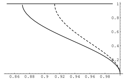
FIG. 1.: PNEC: Outside the horizon. This graph shows the (normalized) critical angle $\psi_{\rm crit}(z)/[\pi/2]$ above which the partial null energy condition fails. (The solid line represents the numerical data; the dotted line represents the Page approximation.)

B Inside the horizon:

Inside the event horizon, one should consider a generic null vector inclined at an angle $\tilde{\psi}$ away from the $t$ direction (which is now spacelike). Then without loss of generality, in an orthonormal frame attached to the $(t,r,\theta,\phi)$ coordinate system,

$$k^{\hat{\mu}}\propto(\cos\tilde{\psi},\pm 1,0,\sin\tilde{\psi}).$$ (61)

One should now consider the quantity

$$T_{\mu\nu}k^{\mu}k^{\nu} \propto (\tau-\rho\cos^{2}\tilde{\psi}+p\sin^{2}\tilde{\psi})$$ (62)

$$= ([\tau-\rho]+[\rho+p]\sin^{2}\tilde{\psi}).$$ (63)

Note that inside the horizon $\tau-\rho$ is strictly positive, while $\rho+p$ is strictly negative. In fact, the Page approximation yields

$$\rho(r)+p(r)=4p_{\infty}\left[1+2\left({2M\over r}\right)+3\left({2M\over r}\right)^{2}+4\left({2M\over r}\right)^{3}+5\left({2M\over r}\right)^{4}+6\left({2M\over r}\right)^{5}-27\left({2M\over r}\right)^{6}\right].$$ (64)

One deduces that violations of the partial null energy condition occur whenever

$$\sin\tilde{\psi}>\sin[\tilde{\psi}_{\rm crit}(r)]\equiv\sqrt{\tau(r)-\rho(r)\over|\rho(r)+p(r)|}$$ (65)

Consequently, violations of the partial null energy condition are confined to the range $\psi\in[\tilde{\psi}_{\rm crit}(r),\pi/2]$. Again defining $z=2M/r$ this critical angle is (in the Page approximation) given by

$$\tilde{\psi}_{\rm crit}(z)=\sin^{-1}\left[\sqrt{{(1-z)(1+3z+6z^{2}+10z^{3}+15z^{4}+21z^{5})\over(1+2z+3z^{2}+4z^{3}+5z^{4}+6z^{5}-27z^{6})}}\right].$$ (66)

One has, at $r=0$, $\tilde{\psi}_{crit}(r=0)=\sin^{-1}\sqrt{7/9}\approx 62\deg$, while $\tilde{\psi}_{\rm crit}$ falls to zero as $r$ approaches $2M$. Qualitatively: near (but inside) the horizon almost all null directions suffer violations of the partial energy condition, while near the central singularity somewhat fewer directions violate the partial null energy condition.

Again, I remind the reader to not take the Page approximation too seriously as one approaches the singularity.

IX Asymptotic null energy condition

I now turn attention to the asymptotic null energy condition (Scri–NEC) that I introduced earlier in this paper. Discussing this energy condition will require some standard results concerning the null geodesics of the Schwarzschild spacetime. (See, for instance, such standard textbooks as Misner–Thorne–Wheeler [36], Wald [37], or Weinberg [38].)

There are two conserved quantities for null geodesic motion in Schwarzschild spacetime; the energy and angular momentum. Using these conservation laws the affine parameter can be chosen in such a way that

$${dt\over d\lambda} = {1\over 1-2M/r};$$ (67)

$${d\phi\over d\lambda} = {a^{2}\over r^{2}}.$$ (68)

The parameter $a$ is the angular momentum per unit energy. If the null geodesic reaches asymptotic spatial infinity then this parameter can also be interpreted as the “impact parameter”. However, there is a large class of null geodesics that never reaches spatial infinity, for these null geodesics the notion of “impact parameter” is at best an abuse of language.

The angle between the null geodesic and the radial direction is given by

$$\sin\psi=\sqrt{1-2M/r}\;\;\left({a\over r}\right).$$ (69)

We are ultimately interested in the quantity

$$T_{\mu\nu}k^{\mu}k^{\nu} \propto ([\rho-\tau]+[\tau+p]\sin^{2}\psi)$$ (70)

$$= \{[\rho-\tau]+[\tau+p](1-2M/r)a^{2}/r^{2}\},$$ (71)

but will need to go through a few preliminaries.

The radial motion of null geodesics is governed by

$$\left({dr\over dt}\right)^{2}=(1-2M/r)^{2}\left[1-(1-2M/r){a^{2}\over r^{2}}\right].$$ (72)

So the turning points, $dr/dt=0$, are given by the cubic

$$r^{2}=a^{2}(1-2M/r).$$ (73)

If the impact parameter is small, $a<3\sqrt{3}M$, then it is a standard result that there are no turning points: the null geodesic either plunges into the future singularity, or emerges from the past singularity of the maximally extended Schwarzschild spacetime. (For $a\lesssim 3\sqrt{3}M$ the geodesic may make a large number of “orbits” before crossing the event horizon.)

If the impact parameter is marginal, $a=3\sqrt{3}M$, then it is a standard result that $r=3M$, corresponding to the (unstable) circular photon orbit.

If the impact parameter is large, $a>3\sqrt{3}M$, then it is a standard result that there are two turning points at physical values of $r$. One of these turning points lies in the range $r\in(3M,\infty)$, while the other lies in the range $r\in(2M,3M)$.

Note that if $a\gg 2M$ then the three mathematical roots of the cubic are approximately $r\approx\pm a-M$, and $r\approx 2M[1+(2M/a)^{2}]$. The two physical roots are approximately $r\approx a-M$ and $r\approx 2M[1+(2M/a)^{2}]$.

The first of these turning points, $r\in(3M,\infty)$, corresponds to the obvious class of null geodesics with high impact parameter—those geodesics that come in from spatial infinity, bounce off the angular momentum barrier, and return to spatial infinity. (For $a\gtrsim 3\sqrt{3}M$ the geodesic may make a large number of “orbits” before returning to spatial infinity.)

The second of these turning points, $r\in(2M,3M)$, corresponds to a completely separate class of null geodesics with high “impact parameter”—these geodesics emerge from the event horizon at $t=-\infty$, with high angular momentum, make a large number of “orbits” before reaching their maximum height above the event horizon, and then make an equally large number of “orbits” before returning to re-cross the event horizon at $t=+\infty$. For these geodesics the use of the phrase “impact parameter” to describe the parameter $a$ is most definitely an abuse of language.

To analyze the asymptotic null energy condition, start by first considering the quantity

$$\Pi(r,a)\equiv(\rho-\tau\cos^{2}\psi+p\sin^{2}\psi),$$ (74)

which I shall refer to as the NEC density. (Remember that $\psi(r,a)$ is an explicitly known function of $r$ and $a$.)

Those null geodesics that come in from infinity and return to infinity never get closer to the origin than $r=3M$. See, for instance, [36, pages 672–678]. Inspection of either the Page approximation or of the numerical data indicates that $\rho$, $-\tau$, and $p$ are all positive for $r\geq 3M$. Thus the asymptotic null energy condition is satisfied along all null geodesics that come from, and return to, infinity.

For other classes of null geodesics it proves convenient to rewrite the quantity $\Pi(r,a)$ as:

$$\Pi(r,a)\equiv\{[\rho-\tau]+[\tau+p](1-2M/r)a^{2}/r^{2}\}.$$ (75)

Now, for incoming null geodesics with smaller than critical impact parameter, the null geodesic may circle the black hole a large number of times, but is guaranteed to ultimately plunge into the event horizon [36, pages 672–678]. This makes the analysis a little more subtle. Inspection of either the Page approximation or the numerical data shows that (outside the horizon) $\rho-\tau$ is always positive, while $\tau+p$ is always negative. Now use the fact that for an infalling null geodesic $a<3\sqrt{3}M$. Since $\tau+p$ is negative, this implies (for this class of null geodesics) a lower bound

$$\Pi(r,a)>L(r)\equiv\{[\rho-\tau]+[\tau+p](1-2M/r)27M^{2}/r^{2}\}.$$ (76)

Inspection of Page’s approximation indicates that this lower bound is strictly positive (zero at the horizon). In fact

$$L(r)=4p_{\infty}\left(1-{2M\over r}\right)\left[1+3\left({2M\over r}\right)+6\left({2M\over r}\right)^{2}+10\left({2M\over r}\right)^{3}+15\left({2M\over r}\right)^{4}+21\left({2M\over r}\right)^{5}-{81\over 2}\left({2M\over r}\right)^{8}\right].$$ (77)

(Note the factorization!) Thus the Page approximation suggests that the asymptotic null energy condition holds on all infalling null geodesics. (At least until one crosses the horizon!) This lower bound $L(r)$ is plotted in figure 2.

By time reversal, this suggests that the asymptotic null energy condition also holds on all outgoing null geodesics that reach infinity.

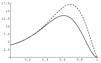
FIG. 2.: L(z): A bound on NEC violations. For all impact parameters $a<3\sqrt{3}M$, the NEC density $\Pi(r,a)$ is bounded below by the quantity $L(r)$, which is itself bounded below by zero. This implies that Scri–NEC is satisfied on all infalling or outfalling null geodesics. (The solid line represents the numerical data; the dotted line represents the Page approximation.)

With respect to the numerical data, one can easily evaluate $L(r)$ numerically. The results are superimposed on figure 2. While there are marked differences between the analytic approximation and the numerical data, both curves are seen to be strictly positive outside the horizon.

We conclude that Scri–NEC is satisfied. For all null geodesics that reach spatial infinity the NEC density $\Pi(r,a)$ is strictly positive everywhere outside the event horizon.

For completeness, and future reference, I point out that the Page approximation yields

$$\Pi(r,a)=4p_{\infty}\left(1-{2M\over r}\right)\left[1+3\left({2M\over r}\right)+6\left({2M\over r}\right)^{2}+10\left({2M\over r}\right)^{3}+15\left({2M\over r}\right)^{4}+21\left({2M\over r}\right)^{5}-{3a^{2}\over 2}\left({2M\over r}\right)^{8}\right].$$ (78)

Again, note the factorization!

X Trapped null geodesics:

Now turn attention to the trapped null geodesics. (These are null geodesics with high “impact parameter” $a>3\sqrt{3}M$, trapped in the region $r\in[2M,3M]$.) While these trapped null geodesics are, by definition, not directly relevant to the Scri–NEC, the tools developed above permit us to gain additional insight into the PNEC on trapped null geodesics.

Pick some value of $r$ in the range $(2M,3M)$. Then $\Pi(r,a)$ is guaranteed to be negative if one chooses

$$a>a_{\rm crit}(r) \equiv \sqrt{{r^{2}(\rho-\tau)\over(1-2M/r)|\tau+p|}}$$ (79)

$$= 2M\sqrt{{(\rho-\tau)\over z^{2}(1-z)|\tau+p|}}.$$ (80)

(Setting $z=2M/r$ is again a convenient choice of variables for both analytic and numeric work. In this section we will only be interested in the region $z\in[2/3,1]$.) Note that what we are doing is guaranteeing that with these definitions the PNEC is violated for the region of the $(a,z)$ plane above the curve $a_{\rm crit}(z)$.

Using Page’s approximation, this critical impact parameter is given by

$$a_{\rm crit}(z)=2M\sqrt{(1+3z+6z^{2}+10z^{3}+15z^{4}+21z^{5})/(6z^{8})}.$$ (81)

The critical impact parameter implied by the numerical data was also determined and both curves are plotted on figure 3.

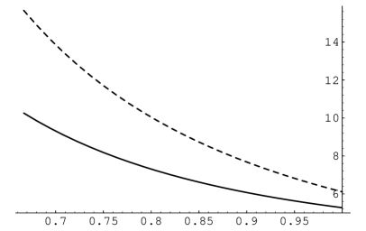
FIG. 3.: $a_{\rm crit}(z)/M$: The critical impact parameter above which NEC is violated on trapped null geodesics. (The solid line represents the numerical data; the dotted line represents the Page approximation.)

It should be noted that, for a given value of $r\in(2M,3M)$, one cannot choose $a$ arbitrarily: In order for a trapped null geodesic with impact parameter $a$ to ever reach radius $r$ it is necessary that $a$ be small enough. Indeed one must have

$$a<a_{\rm max}(r)\equiv\sqrt{{r^{2}\over 1-2M/r}}={2M\over\sqrt{z^{2}(1-z)}}.$$ (82)

This may be thought of as a kinematic bound on trapped null geodesics: the region of the $(a,z)$ plane above the curve $a_{\rm max}(z)$ is kinematically inaccessible to trapped null geodesics. (Note that the region below $a=3\sqrt{3}M$ is also kinematically inaccessible.) The relevant curve is plotted in figures 4 and 5, where it is overlain with $a_{\rm crit}(z)$ as obtained from figure 3. By looking at where these curves cross one another we can draw some general conclusions.

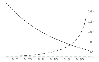
FIG. 4.: Page approximation: The critical impact parameter above which NEC is violated ($a_{\rm crit}(z)/M$)is superimposed on the kinematic bound ($a_{\rm max}(z)/M$). (The dotted line represents the Page approximation; the dashed line represents the kinematic bound.)

In the Page approximation, now restricting attention to the region outside the event horizon:

1. Some trapped null geodesics (those with $a\in[3\sqrt{3}M,2\sqrt{7/3}M]=[5.19615M,6.1101M]$) never experience NEC density violations. That is: $\Pi(r,a)>0$ is satisfied along the entire portion of the null geodesic that lies outside the event horizon. (And therefore the [truncated] ANEC must be satisfied on this entire class of null geodesics.)

2. Some trapped null geodesics (those with $a>7.436M$) always experience NEC density violations. That is: $\Pi(r,a)<0$ along the entire [truncated] null geodesic. (And therefore the [truncated] ANEC must be violated on this entire class of null geodesics.)

3. All other trapped null geodesics (those with $a\in[6.1101M,7.436M]$) will experience some NEC violations when they get sufficiently close to the event horizon. (And therefore investigating ANEC violations on this class of null geodesics requires more work.)

4. Note that $a=6.1101M$ corresponds to a null geodesic that reaches a maximum radius $r_{\rm max}=2.18994M$, a number that we have seen before (when discussing the NEC and PNEC).

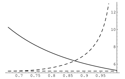
FIG. 5.: Page approximation: The critical impact parameter above which NEC is violated ($a_{\rm crit}(z)/M$)is superimposed on the kinematic bound ($a_{\rm max}(z)/M$). (The solid line represents the numerical data; the dashed line represents the kinematic bound.)

Use of the numerical data implies quantitative though not qualitative changes. We observe that

1. The set of trapped null geodesics which never experience NEC density violations is much smaller—those with $a\in[3\sqrt{3}M,5.276M]=[5.19615M,5.276M]$. (The [truncated] ANEC must be satisfied on this entire class of null geodesics.)

2. Some trapped null geodesics (those with $a>6.383M$) always experience NEC density violations. (Therefore the [truncated] ANEC must be violated on this entire class of null geodesics.)

3. All other trapped null geodesics (those with $a\in[5.276M,6.383M]$) will experience some NEC violations when they get sufficiently close to the event horizon. (And therefore investigating ANEC violations on this class of null geodesics requires more work.)

4. Note that $a=6.383M$ corresponds to null geodesic that reaches a maximum radius $r_{\rm max}=2.298M$, a number that we have seen before (when discussing the PNEC).

The message to be extracted is this: The numeric data and analytic approximations are in good qualitative agreement with each other. Null geodesics that reach null infinity are well behaved (Scri–NEC is satisfied), but some of the trapped null geodesics encounter NEC violations (and ANEC violations).

XI Averaged null energy condition

We are finally in a position to pin down precisely violations of the ANEC itself. Although significant information can already be extracted by using the point-wise energy conditions already discussed, beyond a certain stage explicit use of the affine parameterization must be invoked. Write the ANEC integral as [6, page 117]

$$I_{\gamma} \equiv \int_{\gamma}T_{\mu\nu}\;k^{\mu}\;k^{\nu}\;d\lambda,$$ (83)

$$= \int_{\gamma}(\rho-\tau\cos^{2}\psi+p\sin^{2}\psi)\;\xi^{2}\;d\lambda,$$ (84)

$$= \int_{\gamma}([\rho-\tau]+[\tau+p]\sin^{2}\psi)\;\xi^{2}\;d\lambda,$$ (85)

$$= \int_{\gamma}\Pi(r,a)\;\xi^{2}\;d\lambda.$$ (86)

Note that the integrand is proportional to the quantity $\Pi(r,a)$ which has already been extensively discussed in the context of the Scri–NEC.

A Scri–ANEC

The arguments previously adduced for the Scri–NEC can be carried over wholesale to the Scri–ANEC. In particular:

• For null geodesics that come in from spatial infinity and return to spatial infinity $(a>3\sqrt{3}M;r>3M)$ the integrand is everywhere positive and so the ANEC holds on this entire class of geodesics. (Note that satisfaction of the ANEC does not arise from the trivial observation that the heat bath contributes an asymptotically constant and positive energy density far from the black hole—rather one has the stronger statement that the integrand itself is positive along the entire geodesic.)

• The fact that the integrand is positive implies that ANEC will also be satisfied for curves with transverse smearing [7], or curves with arbitrary positive weighting functions [11].

• For infalling or outfalling null geodesics that reach asymptotic spatial infinity $(a<3\sqrt{3}M;r\in(2M,\infty))$ the integrand is everywhere positive and ANEC is satisfied. [Caveat: I stop the ANEC integral once it reaches the horizon.]

• This may be interpreted as follows: Because Scri–NEC is satisfied, it automatically follows that Scri–ANEC is satisfied.

• For the unstable circular photon orbit $(a=3\sqrt{3}M;r=3M)$ the integrand is everywhere positive and ANEC is satisfied.

• However, for trapped null geodesics $(a>3\sqrt{3}M;r\in[2M,3M])$ the integrand is no longer necessarily positive, and this is the only case for which we will explicitly need to look at the “weighting function” $\xi^{2}d\lambda$ appearing in the ANEC integral.

B ANEC on trapped null geodesics?

Observe that the “weighting function” appearing in the ANEC satisfies [6, page 133, equations (12.60)–(12.63)]

$$\xi^{2}d\lambda=g_{00}\left({dt\over d\lambda}\right)^{2}d\lambda=(1-2M/r)\left({1\over 1-2M/r}\right)^{2}(1-2M/r)dt=dt.$$ (87)

Although this calculation was carried out for the Schwarzschild geometry the result remains true for an arbitrary static spacetime—the ANEC integral is simply the time-average along a null geodesic of the local-Lorentz NEC integrand where the time average is to be taken with respect to the natural static time coordinate.

For actual calculations it is much more practical to re-express this as an integral with respect to the radial variable $r$ by using

$${dr\over\sqrt{1-2M/r}}=\cos\psi\;dt\;\sqrt{1-2M/r},$$ (88)

so that

$$dt={dr\over\cos\psi\;(1-2M/r)}={dr\over(1-2M/r)\;\sqrt{1-(1-2M/r)a^{2}/r^{2}}}.$$ (89)

Now this observation appears to weight the region near the event horizon very heavily—because of the explicit pole at $r=2M$. However, the integrand $\Pi(r,a)$ has a zero at the event horizon—in the Page approximation one discovers an explicit factor of $(1-2M/r)$ [Cf. equation 78], while the numerical data also exhibits a first-order zero in $\Pi(r,a)$ at the horizon. Thus for trapped null geodesics one may write

$$I_{\gamma}(a)=2\int_{2M}^{r_{\rm max}(a)}{\Pi(r,a)\over(1-2M/r)}\;{dr\over\sqrt{1-(1-2M/r)a^{2}/r^{2}}},$$ (90)

and have some confidence that the integral actually converges at the lower bound $r=2M$. As a penultimate step, recall that calculating $r_{\rm max}(a)$ involves solving a cubic. It is more convenient to parameterize the trapped geodesic by calculating the impact parameter in terms of the maximum height attained by the null geodesic:

$$a(r_{\rm max})={r_{\rm max}\over\sqrt{1-2M/r_{\rm max}}}.$$ (91)

So for these trapped null geodesics one finds the ANEC integral is

$$I_{\gamma}(r_{\rm max})=2\int_{2M}^{r_{\rm max}}{\Pi(r,r_{\rm max})\over(1-2M/r)}\;{dr\over\sqrt{1-[(1-2M/r)r_{\rm max}^{2}]/[(1-2M/r_{\rm max})r^{2}]}},$$ (92)

To actually evaluate this integral numerically it is useful to change variables to $z=2M/r$, and $z_{0}=2M/r_{\rm max}$, with the result that

$$I_{\gamma}(z_{0})=4M\int_{z_{0}}^{1}{\Pi(z,z_{0})\over z^{2}(1-z)}\;{dz\over\sqrt{1-[z^{2}(1-z)]/[z_{0}^{2}(1-z_{0})]}},$$ (93)

With a little work, the square root can be seen to factorize explicitly

$$I_{\gamma}(z_{0})=4Mz_{0}\sqrt{1-z_{0}}\;\int_{z_{0}}^{1}{\Pi(z,z_{0})\over z^{2}(1-z)}\;{1\over\sqrt{z^{2}+z_{0}^{2}+zz_{0}-z-z_{0}}}\;{dz\over\sqrt{z-z_{0}}},$$ (94)

This integral, though singular at the lower limit ($z=z_{0}$, corresponding to $r=r_{\rm max}$), is now certainly finite. While Mathematica has resources to deal with $1/\sqrt{z}$ singularities at the endpoints of the integration range, it reacts badly to such singularities when the location is chosen dynamically. That is: $\int_{z_{0}}^{1}1/\sqrt{z-z_{0}}$ is handled badly. For this reason the change of variables $z=z_{0}+w$, while being a formal mathematical identity, leads to much better numerical behaviour for the integral:

$$I_{\gamma}(z_{0})=4Mz_{0}\sqrt{1-z_{0}}\;\int_{0}^{1-z_{0}}{\Pi(z_{0}+w,z_{0})\over(z_{0}+w)^{2}(1-w-z_{0})}\;{1\over\sqrt{(z_{0}+w)^{2}+z_{0}^{2}+(z_{0}+w)z_{0}-(z_{0}+w)-z_{0}}}\;{dw\over\sqrt{w}}.$$ (95)

This integral was determined numerically both for the Page approximation and for the Anderson–Hiscock–Samuel numeric data. The results are graphed in figure 6. Remember that it is meaningless to force this particular integral out of the range $r\in[2M,3M]$, corresponding to $z_{0}\in[2/3,1]$

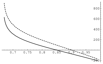
FIG. 6.: ANEC integral on trapped null geodesics: The ANEC integral has been evaluated numerically as a function of $z_{0}=2M/r_{\rm max}$. (The solid line represents the numerical data; the dotted line represents the Page approximation.)

Thus we have (finally!) managed to characterize the precise class of null geodesics on which the [truncated] ANEC is violated.

The critical values of $z_{0}$, $r_{\rm max}$, and $a$ are, for the Page approximation:

$$z_{0} = 0.90083;$$ (96)

$$r_{\rm max} = 2.2202\;M;$$ (97)

$$a = 7.0501\;M.$$ (98)

For the numerical data, one obtains:

$$z_{0} = 0.8497;$$ (99)

$$r_{\rm max} = 2.354\;M;$$ (100)

$$a = 6.071\;M.$$ (101)

Note that these numbers are qualitatively reasonable and in agreement with the violations of the point-wise energy conditions, and the numerical investigation of the PNEC. Furthermore the ANEC violations in the numerical data are seen to extend out to larger distances than the ANEC violations in the Page approximation, in agreement with the general trend.

Though I have quoted four-significant-digit accuracy for the numerical data one should probably not take anything past the second significant digit too seriously. In fact, given the vagaries of numerical analysis on singular integrals (and the inherent uncertainties in the Anderson–Hiscock–Samuel data) it is conceivable that the exact critical impact parameters might be $a=7M$ and $a=6M$ respectively.

C ANEC on non-geodesic curves?

If one considers arbitrary non-geodesic curves the ANEC loses much (though not quite all) of its power: by a judicious choice of non-geodesic null curve one could try to remain in a region where the NEC is violated and thereby “trivially” violate the ANEC [19].

For instance, along any circular null curve at fixed $r$ (not a geodesic except in the case of $r=3M$) the ANEC integral is still proportional to $\rho+p$. Inspection of the numeric data indicates that $\rho+p<0$ for $r\lesssim 2.298\,M$. (Page’s analytic approximation giving a slightly different result, $\rho+p<0$ for $r<2.18994\,M$.) Thus the ANEC is not satisfied for this particular class of non–geodesic null curves.

XII Discussion

Investigation of the properties of the averaged null energy condition is of considerable interest to diverse applications in semiclassical quantum gravity. It is now abundantly clear that, in the test-field limit, semiclassical quantum fields do not generally satisfy the ANEC: Indeed ANEC violations are related to the existence of a non-zero scale anomaly [6, 20]. Even if the scale anomaly vanishes, this does not necessarily imply that the ANEC is satisfied: one has to do a case by case analysis. As an example, this paper investigates the situation in Schwarzschild spacetime.

The analysis presented herein is somewhat of an attempt to crack a walnut with a sledgehammer in the sense that it is a collection of rather general techniques applied to a rather particular problem—it is certainly true that this type of analysis can now be carried forward to other geometries, other quantum fields, and other vacuum states by by straightforward but tedious computation.

For the Schwarzschild geometry (with a conformally coupled scalar field in the Hartle–Hawking vacuum) the results may be expressed thusly:

• Point-wise energy conditions—

  • Inside the event horizon, with suitable caveats regarding the applicability of the Page approximation, almost any energy condition you can think of will be violated.

  • Between the event horizon $(r=2M)$ and the unstable photon orbit $(r=3M)$ many of the energy conditions are violated, in a series of onion-like layers.

  • Outside the unstable photon orbit $(r=3M)$ all energy conditions are satisfied.

  • All null geodesics that reach asymptotic infinity are well-behaved: If you look along the null geodesic you never see NEC violations.

• Averaged null energy condition—

  • If your null geodesic ever reaches infinity, the [truncated] ANEC is definitely satisfied, and is satisfied for a non-trivial reason: the integrand is strictly positive all the way from the event horizon to null infinity.

  • Between the event horizon $(r=2M)$ and the unstable photon orbit $(r=3M)$ some of the trapped null geodesics violate the [truncated] ANEC.

  • If you are willing to look at non-geodesic null curves even more violations of the ANEC can be found.

It should be possible to generalize the observations of this paper. For instance:

1. It would be very nice to have an analytic understanding of the precise role played by the unstable photon orbit—the numerical evidence is suggestive but not definitive.

2. For that matter it would be nice to know if the relevance of the unstable photon orbit generalizes to other geometries.

3. It would be nice to go beyond the numerics; to develop some exact analytic arguments that go beyond the Page approximation.

4. Generalizations to the Boulware vacuum will be presented in a companion paper.

5. Generalizations to the Unruh vacuum, other quantum fields, non-conformal couplings, particle masses, and the Reissner–Nordström geometry will be straightforward if tedious.

6. The new energy conditions I introduce, Scri–NEC and Scri–ANEC, are interesting in that they focus attention on null infinity. And null infinity is where all the interesting details arise in the Friedman–Schleich–Witt [22] topological censorship theorem, and the Penrose–Sorkin–Woolgar version of the positive mass theorem [21]. I suspect that with a little more work suitable generalizations of these theorems can be constructed in terms of the Scri–ANEC.

7. Finally I should point out that even though the various energy conditions are violated in many regions, this does not give one a completely free hand to design spacetime geometries to taste: It seems quite likely that the “quantum inequality” approach of Ford and Roman [39, 40] will allow us to place constraints on spacetime geometries even if all the usual types of energy condition fail.

REFERENCES

- [1] B. S. DeWitt. Quantum field theory in curved spacetime. Phys. Rep., 19:295–357, 1975. See especially pp. 342–345.
- [2] S. W. Hawking and W. Israel, editors. General Relativity: An Einstein Centenary Survey. Cambridge University Press, Cambridge, England, 1979.
- [3] N. D. Birrell and P. C. W. Davies. Quantum Fields in Curved Space. Cambridge University Press, Cambridge, England, 1982.
- [4] S. W. Hawking and W. Israel, editors. 300 Years of Gravitation. Cambridge University Press, Cambridge, England, 1987.
- [5] S. A. Fulling. Aspects of Quantum Field Theory in Curved Space–Time. Cambridge University Press, Cambridge, England, 1989.
- [6] M. Visser. Lorentzian wormholes — from Einstein to Hawking. American Institute of Physics, New York, 1995.
- [7] É. É. Flanagan and R. M. Wald. Does backreaction enforce the averged null energy condition in semiclassical gravity? gr-qc/9602052, 1996.
- [8] G. T. Horowitz. Semiclassical relativity: The weak–field limit. Phys. Rev. D, 21:1455–1461, 1980.
- [9] G. T. Horowitz and R. M. Wald. Quantum stress tensor in nearly conformally flat spacetimes. Phys. Rev. D, 21:1462–1465, 1980.
- [10] L. H. Ford and T. A. Roman. Motion of inertial observers through negative energy. Phys. Rev. D, 48:776–782, 1993.
- [11] L. H. Ford and T. A. Roman. Averaged energy conditions and evaporating black holes. Phys. Rev. D, 53:1988–2000, 1996.
- [12] D. N. Page. Thermal stress tensor in Einstein spaces. Phys. Rev. D, 25:1499–1509, 1982. Reprinted in [41].
- [13] K. W. Howard. Vacuum in Schwarzschild spacetime. Phys. Rev. D, 30:2532–2547, 1984.
- [14] K. W. Howard and P. Candelas. Quantum stress tensor in Schwarzschild space-time. Phys. Rev. Lett., 53:403–406, 1984. Reprinted in [41].
- [15] P. R. Anderson, W. A. Hiscock, and D. A. Samuel. Stress–energy tensor of quantized scalar fields in static black hole spacetimes. Phys. Rev. Lett., 70:1739–1742, 1993.
- [16] P. R. Anderson, W. A. Hiscock, and D. A. Samuel. Stress-energy tensor of quantized scalar fileds in static spherically symmetric spacetimes. Phys. Rev., D51:4337–4358, 1995.
- [17] P. Anderson. Private communication.
- [18] S. W. Hawking and G. F. R. Ellis. The Large Scale Structure of Space-Time. Cambridge University Press, Cambridge, England, 1973.
- [19] G. Klinkhammer. Averaged energy conditions for free scalar fields in flat spacetime. Phys. Rev. D, 43:2542–2548, 1991.
- [20] M. Visser. Scale anomalies imply violation of the averaged null energy condition. Phys. Lett., B349:443–447, 1995.
- [21] R. Penrose, R. D. Sorkin, and E. Woolgar. A positive mass theorem based on the focusing and retardation of null geodesics. 1993. gr-qc/9301015.
- [22] J. L. Friedman, K. Schleich, and D. M. Witt. Topological censorship. Phys. Rev. Lett., 71:1486–1489, 1993.
- [23] M. R. Brown and A. C. Ottewill. Effective actions and conformal transformations. Phys. Rev. D, 31:2514–2520, 1985.
- [24] T. Elster. Vacuum polarization near a black hole creating particles. Phys. Lett., 94 A:205–209, 1983.
- [25] M. R. Brown, A. C. Ottewill, and D. N. Page. Conformally invariant quantum field theory in static Einstein space-times. Phys. Rev. D, 33:2840–2850, 1986.
- [26] P. Candelas and K. W. Howard. Vacuum in Schwarzschild spacetime. Phys. Rev. D, 29:1618–1625, 1984.
- [27] V. P. Frolov and K. S. Thorne. Renormalized stress–energy tensor near the horizon of a slowly evolving, rotating black hole. Phys. Rev. D, 39:2125–2154, 1989.
- [28] S. M. Christensen and S. A. Fulling. Trace anomalies and the Hawking effect. Phys. Rev. D, 15:2088–2104, 1977.
- [29] P. Candelas, P. Chrzanowski, and K. W. Howard. Quantization of electromagnetic and gravitational perturbations of a Kerr black hole. Phys. Rev. D, 24:297–304, 1981.
- [30] B. P. Jensen and A. C. Ottewill. Renormalized electromagnetic stress tensor in Schwarzschild spacetime. Phys. Rev. D, 39:1130–1138, 1989.
- [31] V. P. Frolov and A. I. Zel’nikov. Killing approximation for vacuum and thermal stress–energy tensor in static space-times. Phys. Rev. D, 35:3031–3044, 1987.
- [32] T. Elster. Quantum vacuum energy near a black hole: the Maxwell field. Class. Quantum Grav., 1:43–54, 1984.
- [33] B. P. Jensen, J. G. McLauglin, and A. C. Ottewill. Renormalized elecromagnetic stress for an evaporating black hole. Phys. Rev. D, 43:4142–4144, 1991.
- [34] B. P. Jensen, J. G. McLauglin, and A. C. Ottewill. Anisotropy of the quantum thermal state in Schwarzschild spacetime. Phys. Rev. D, 45:3002–3005, 1992.
- [35] J. Matyjasek. Hadamard regularization in Schwarzschild spacetime: Israel–hartle–hawking vacuum. Phys. Rev. D, 53:794–800, 1996.
- [36] C. W. Misner, K. S. Thorne, and J. A. Wheeler. Gravitation. W. H. Freeman and Company, San Francisco, 1973.
- [37] R. M. Wald. General Relativity. University of Chicago Press, Chicago, 1984.
- [38] S. Weinberg. Gravitation and Cosmology. Wiley, New York, 1972.
- [39] L. H. Ford and T. A. Roman. Averaged energy conditions and quantum inequalities. Phys. Rev. D, 51:4277–4286, 1995.
- [40] L. H. Ford and T. A. Roman. Averaged energy conditions constrain traversable wormhole geometries. gr-qc/9510071, 1995.
- [41] S. W. Hawking and G. W. Gibbons, editors. Euclidean Quantum Gravity. World Scientific, Singapore, 1993.