Numerical Investigation of Singularities

Abstract

Numerical exploration of the properties of singularities could, in principle, yield detailed understanding of their nature in physically realistic cases. Examples of numerical investigations into the formation of naked singularities, critical behavior in collapse, passage through the Cauchy horizon, chaos of the Mixmaster singularity, and singularities in spatially inhomogeneous cosmololgies are discussed.

1 Introduction

The singularity theorems [1, 2, 3, 4] state that Einstein’s equations will not evolve regular initial data arbitrarily far into the future or the past. An obstruction such as infinite curvature or the termination of geodesics will always arise to stop the evolution somewhere. The simplest, physically relevant solutions representing for example a homogeneous, isotropic universe (Friedmann-Robertson-Walker (FRW)) or a spherically symmetric black hole (Schwarzschild) contain space-like infinite curvature singularities. Although, in principle, the presence of a singularity could lead to unpredictable measurements for a physically realistic observer, this does not happen for these two solutions. The surface of last scattering of the cosmic microwave background in the cosmological case and the event horizon in the black hole (BH) case effectively hide the singularity from present day, external observers. The extent to which this “hidden” singularity is generic and the types of singularities that appear in generic spacetimes remain major open questions in general relativity. The questions arise quickly since other exact solutions to Einstein’s equations have singularities which are quite different from those described above. For example, the charged BH (Reissner-Nordstrom solution) has a time-like singularity. It also contains a Cauchy horizon (CH) marking the boundary of predictability of space-like initial data. A test observer can pass through the CH to another region of the extended spacetime. More general cosmologies can exhibit singularity behavior different from that in FRW. The Big Bang in FRW is classified as an asymptotically velocity term dominated (AVTD) singularity [5, 6] since any spatial curvature term in the Hamiltonian constraint becomes negligible compared to the square of the expansion rate as the singularity is approached. However, some anisotropic, homogeneous models exhibit Mixmaster dynamics (MD) [7, 8] and are not AVTD—the influence of the spatial scalar curvature can never be neglected.

Once the simplest, exactly solvable models are left behind, understanding of the singularity becomes more difficult. Other chapters [9, 10] describe recent analytic progress. However, such methods yield either detailed knowledge of unrealistic, simplified (usually by symmetries) spacetimes or powerful, general results that do not contain details. To overcome these limitations, one might consider numerical methods to evolve realistic spacetimes to the point where the properties of the singularity may be identified. Of course, most of the effort in numerical relativity applied to BH collisions has addressed the avoidance of singularities.[11] One wishes to keep the computational grid in the observable region outside the horizon. Much less computational effort has focused on the nature of the singularity itself. Numerical calculations, even more than analytic ones, require finite values for all quantities. Ideally then, one must describe the singularity by the asymptotic non-singular approach to it. A numerical method which can follow the evolution into this asymptotic regime will then yield information about the singularity. Since the numerical study must begin with a particular set of initial data, the results can never have the force of mathematical proof. One may hope, however, that such studies will provide an understanding of the “phenomenology” of singularities that will eventually guide and motivate rigorous results.

In the following, we shall consider examples of numerical study of singularities both for asymptotically flat (AF) spacetimes and for cosmological models. These examples have been chosen to illustrate primarily numerical studies whose focus is the nature of the singularity itself. In the AF context, we shall consider two questions. The first is whether or not naked singularities exist for realistic matter sources. One approach is to explore highly non-spherical collapse looking for spindle or pancake singularities. If the formation of an event horizon requires a limit on the aspect ratio of the matter,[12] such configurations may yield a naked singularity. Another approach is to probe the limits between initial configurations which lead to black holes and those which yield no singularity at all (i.e. flat spacetime plus radiation) to explore the singularity as the BH mass goes to zero. This quest led naturally to the discovery of critical behavior in the collapse of a scalar field.[13] The other question which is now beginning to yield to numerical attack involves the stability of the Cauchy horizon in charged or rotating black holes where it has been conjectured [1, 14] that a real observer, as opposed to a test mass, cannot pass through the CH since realistic perturbed spacetimes will convert the CH to a true singularity. In cosmology, we shall consider both the behavior of the Mixmaster model and the issue of whether or not its properties are applicable to generic cosmological singularities. Although numerical evolution of the Mixmaster equations has a long history, recent developments are motivated by inconsistencies between the known sensitivity to initial conditions and standard measures of the chaos usually associated with such behavior.[15, 16, 17, 18, 19, 20, 21] Belinskii, Khalatnikov, and Lifshitz (BKL) long ago claimed [7] that it is possible to formulate the generic cosmological solution to Einstein’s equations near the singularity as a Mixmaster universe at every point. While others have questioned the the validity of this claim,[22] there is as yet no evidence either way for such behavior in spatially inhomogeneous cosmologies. We shall discuss a numerical program to address this issue.

2 Singularities in AF spacetimes

2.1 Naked singularities and the hoop conjecture

The strong cosmic censorship conjecture [23] requires a singularity formed from regular, asymptotically flat initial data to be hidden from an external observer by an event horizon. Counter examples have been known for a long time but tend to be dismissed as unrealistic in some way. The goal of a numerical approach is to try to search for naked singularities arising from physically reasonable initial conditions. A possible regime for such systems is motivated by Thorne’s “hoop conjecture” [12] that collapse will yield a black hole only if a mass $M$ is compressed to a region with circumference $C\leq 4\pi M$ in all directions. (Note that one must take care to define $C$ and $M$ especially if the initial data are not at least axially symmetric.) If the hoop conjecture is true, naked singularities may form if collapse can yield $C\geq 4\pi M$ in some direction. The existence of a naked singularity is inferred from the absence of an apparent horizon (AH) which can be identified locally by following null geodesics. Although a definitive identification of a naked singularity requires the event horizon (EH) to be proven to be absent, to identify an EH requires knowledge of the entire spacetime. Methods to find an EH in a numerically determined spacetime have only recently become available and have not been applied to this issue.[26] To attempt to produce naked singularities, Shapiro and Teukolsky (ST) [24] considered collapse of prolate spheroids of collisionless gas. (Nakamura and Sato [25] had previously studied the collapse of non-rotating deformed stars with an initial large reduction of internal energy and apparently found spindle or pancake singularities in extreme cases.) ST solved the general relativistic Vlasov equation for the particles along with Einstein’s equations for the gravitational field. Null geodesics were followed to identify an AH if present. The curvature invariant $I=R_{\mu\nu\rho\sigma}R^{\mu\nu\rho\sigma}$ was also computed. They found that an AH (and presumably a BH) formed if $C\leq 4\pi M<1$ everywhere but no AH (and presumably a naked singularity) in the opposite case. In the latter case, the evolution (not surprisingly) could not proceed past the moment of formation of the singularity. In a subsequent study, ST [29] also showed that a small amount of rotation (counter rotating particles with no net angular momentum) does not prevent the formation of a naked spindle singularity. However, Wald and Iyer [27] have shown that the Schwarzschild solution has a time slicing whose evolution approaches arbitrarily close to the singularity with no AH in any slice (but,of course, with an EH in the spacetime). This may mean that there is a chance that the increasing prolateness found by ST in effect changes the slicing to one with no apparent horizon just at the point required by the hoop conjecture. While, on the face of it, this seems unlikely, Tod gives an example where the AH does not form on a chosen constant time slice—but rather different portions form at different times. He argues that a numerical simulation might be forced by the singularity to end before the formation of the AH is complete. Such an AH would not be found by the simulations.[28] In response, Shapiro and Teukolsky considered equilibrium sequences of prolate relativistic star clusters.[30] The idea is to counter the possibility that an EH might form after the simulation must stop. If an equilibrium configuration is non-singular, it cannot contain an EH since singularity theorems say that an EH implies a singularity. However, a sequence of non-singular equilibria with rising $I$ ever closer to the spindle singularity would lend support to the existence of a naked spindle singularity since one can approach the singular state without formation of an EH. They constructed this sequence and found that the singular end points were very similar to their dynamical spindle singularity.

Motivated by ST’s results,[24] Echeverria [31] numerically studied the properties of the naked singularity that is known to form in the collapse of an infinite, cylindrical dust shell.[12] While the asymptotic state can be found analytically, the approach to it must be followed numerically. The analytic asymptotic solution can be matched to the numerical one (which cannot be followed all the way to the collapse) to show that the singularity is strong (an observer experiences infinite stretching parallel to the symmetry axis and squeezing perpendicular to the symmetry axis). A burst of gravitational radiation emitted just prior to the formation of the singularity can be studied.

A very recent numerical study of the hoop conjecture was made by Chiba et al.[32] Rather than a dynamical collapse model, they searched for AH’s in analytic initial data for discs, annuli, and rings. Previous studies of this type were done by Nakamura et al [33] with oblate and prolate spheroids and by Wojtkiewicz [34] with axisymmetric singular lines and rings. The summary of their results is that an AH forms if $C\leq 4\pi M\leq 1.26$. (Analytic results due to Barrabès et al [35, 36] and Tod [28] give similar quantitative results with different initial data classes and (possibly) definition of $C$.) The results of all these searches for naked singularities are controversial but could be resolved if the presence or absence of the EH could be determined.

2.2 Critical behavior in collapse

We now consider an effect that was originally found by Choptuik [13] in a numerical study of the collapse of a spherically symmetric massless scalar field. We note that this is the first completely new phenomenon in general relativity to be discovered by numerical simulation. In collapse of a scalar field, essentially two things can happen: either a BH forms or the scalar waves pass through each other and disperse. Choptuik discovered that for any 1-parameter set of initial data labeled by $p$, there is a critical value $p^{\ast}$ such that $p>p^{\ast}$ yields a BH. He found

$$M_{BH}\approx C_{F}\left(p-p^{\ast}\right)^{\gamma}$$ (1)

where $M_{BH}$ is the mass of the eventual BH. The constant $C_{F}$ depends on the parameter of the initial data that is selected but $\gamma\approx.37$ is the same for all choices. Furthermore, in terms of logarithmic variables $\rho=\ln r+\kappa$, $\tau=\ln(T_{0}^{\ast}-T_{0})+\kappa$ ($T_{0}$ is the proper time of an observer at $r=0$ with $T_{0}^{\ast}$ the finite proper time at which the critical evolution concludes), the waveform $X$ repeats (echoes) at intervals of $\Delta$ in $\tau$ if $\rho$ is rescaled to $\rho-\Delta$, i.e. $X(\rho-\Delta,\tau-\Delta)\approx X(\rho,\tau)$. The scaling behavior (1) demonstrates that the minimum BH mass (for bosons) is zero. The critical solution itself is a counter-example to cosmic censorship (since the formation of the zero mass BH causes high curvature regions become visible at $r=\infty$). (See, e.g., the discussion in Hirschmann and Eardley.[37])

Soon after this discovery, scaling and critical phenomena were found in a variety of contexts. Abrahams and Evans [38] discovered the same phenomenon in axisymmetric gravitational wave collapse with a different value of $\Delta$ and, to within numerical error, the same value of $\gamma$. (Note that the rescaling of $r$ with $e^{\Delta}\approx 30$ required Choptuik to use adaptive mesh refinement (AMR) to distinguish subsequent echoes. Abrahams and Evans’ smaller $\Delta$ ($e^{\Delta}\approx 1.8$) allowed them to see echoing with their $2+1$ code without AMR.) Recently, Garfinkle [39] has confirmed Choptuik’s results with a completely different algorithm that does not require AMR. His use of Goldwirth and Piran’s [40] method of simulating Christodoulou’s [41] formulation of the spherically symmetric scalar field in null coordinates allowed the grid to be automatically rescaled by choosing the edge of the grid to be the null ray that just hits the central observer at the end of the critical evolution. (Missing points of null rays that cross the central observer’s world line are replaced by interpolation between those that remain.) Hamadé and Stewart [42] have also repeated Choptuik’s calculation using null coordinates and AMR. They are able to achieve greater accuracy and find $\gamma=.374$.

Evans and Coleman [43] realized that self-similar rather than self-periodic collapse might be more tractable both numerically (since ODE’s rather than PDE’s are involved) and analytically. They discovered that a collapsing radiation fluid had that desirable property. (Note that self-similarity (homothetic motion) is incompatible with AF. However, most of the action occurs in the center so that a match of the self-similar inner region to an outer AF one should always be possible.) In a series of papers, Hirschmann and Eardley [37, 44] developed a (numerical) self-similar solution to the spherically symmetric complex scalar field equations. These are ODE’s with too many boundary conditions causing a solution to exist only for certain fixed values of $\Delta$. Numerical solution of this eigenvalue problem allows very accurate determination of $\Delta$. The self-similarity also allows accurate calculation of $\gamma$ as follows: The critical $p=p^{\ast}$ solution is unstable to a small change in $p$. At any time $t$ (where $t<0$ is increasing toward zero), the amplitude $a$ of the perturbation exhibits power law growth:

$$a\propto(p-p^{\ast})(-t)^{-\kappa}$$ (2)

where $\kappa>0$. At any fixed $t$, larger $a$ implies larger $M_{BH}$. Equivalently, any fixed amplitude $a=\delta$ will be reached faster for larger eventual $M_{BH}$. Scaling arguments give the dependence of $M_{BH}$ on the time at which any fixed amplitude is reached:

$$M_{BH}\propto(-t_{1})$$ (3)

where

$$(p-p^{\ast})(-t_{1})^{\kappa}\propto\delta.$$ (4)

Thus

$$M_{BH}\propto(p-p^{\ast})^{1/\kappa}.$$ (5)

Therefore, one need only identify the growth rate of the unstable mode to obtain an accurate value of $\gamma=1/\kappa$. It is not necessary to undertake the entire dynamical evolution or probe the space of initial data. Hirschmann and Eardley obtain $\gamma=0.387106$ for the complex scalar field solution while Koiki et al [45] obtain $\gamma=0.35580192$ for the Evans-Coleman solution. Although the similarities among the critical exponents $\gamma$ in the collapse computations suggested a universal value, Maison [46] used these same scaling-perturbation methods to show that $\gamma$ depends on the equation of state $p=k\rho$ of the fluid in the Evans-Coleman solution. Very recently, Gundlach [47] used a similar approach to locate Choptuik’s critical solution accurately. This is much harder due to its discrete self-similarity. He reformulates the model as nonlinear hyperbolic boundary value problem with eigenvalue $\Delta$ and finds $\Delta=3.4439$. As with the self-similar solutions described above, the critical solution is found directly without the need to perform a dynamical evolution or explore the space of initial data. Perturbation of this solution could yield an accurate value of $\gamma$.

2.3 Nature of the singularity in charged or rotating black holes

Unlike the simple singularity structure of the Schwarzschild solution, where the event horizon encloses a spacelike singularity at $r=0$, charged and/or rotating BH’s have a much richer singularity structure. The extended spacetimes have an inner Cauchy horizon (CH) which is the boundary of predictability. To the future of the CH lies a timelike (ring) singularity.[1] Poisson and Israel [48, 49] began an analytic study of the effect of perturbations on the CH. Their goal was to check conjectures that the blue-shifted infalling radiation during collapse would convert the CH into a true singularity and thus prevent an observer’s passage into the rest of the extended regions. By including both ingoing and back-scattered outgoing radiation, they find for the Reissner-Nordstrom (RN) solution that the mass function (qualitatively $R_{\alpha\beta\gamma\delta}\propto M/r^{3}$) diverges at the CH (mass inflation). However, Ori showed both for RN and Kerr [50, 51] that the metric perturbations are finite (even though $R_{\mu\nu\rho\sigma}R^{\mu\nu\rho\sigma}$ diverges) so that an observer would not be destroyed by tidal forces (the tidal distortion would be finite) and could survive passage through the CH. A numerical solution of the Einstein-Maxwell-scalar field equations could test these perturbative results.

Gnedin and Gnedin [52] have numerically evolved the spherically symmetric Einstein-Maxwell with massless scalar field equations in a $2+2$ formulation. The initial conditions place a scalar field on part of the RN event horizon (with zero field on the rest). An asymptotically null or spacelike singularity whose shape depends on the strength of the initial perturbation replaces the CH. For a sufficiently strong perturbation, the singularity is Schwarzschild-like. Although they claim to have found that the CH evolved to become a spacelike singularity, the diagrams in their paper show at least part of the final singularity to be null or asymptotically null in most cases.

Brady and Smith [53] used the Goldwirth-Piran formulation [40] to study the same problem. They assume the spacetime is RN for $v<v_{0}$. They follow the evolution of the CH into a null singularity, demonstrate mass inflation, and support (with observed exponential decay of the metric component $g$) the validity of previous analytic results [48, 49, 50, 51] including the “weak” nature of the singularity that forms. They find that the observer hits the null CH singularity before falling into the curvature singularity at $r=0$. Whether or not these results are in conflict with Gnedin and Gnedin [52] is unclear.[54]

We finally mention Hübner’s [55] numerical scheme to evolve on a conformal compactified grid using Friedrich’s formalism.[56] He considers the spherically symmetric scalar field model in a $2+2$ formulation. So far, this code has been used to locate singularities and to identify Choptuik’s scaling.[13]

3 Singularities in cosmological models

3.1 Mixmaster dynamics

Belinskii, Khalatnikov, and Lifshitz [7] (BKL) described the singularity approach of vacuum Bianchi IX cosmologies as an infinite sequence of Kasner epochs whose indices change when the scalar curvature terms in Einstein’s equations become important. They were able to describe the dynamics approximately by a map evolving a discrete set of parameters from one Kasner epoch to the next.[7, 57] For example, the Kasner indices for the power law dependence of the anisotropic scale factors can be parametrized by a single variable $u\geq 1$. BKL determined that

$$u_{n+1}=\left\{\matrix{u_{n}-1\quad\quad,\quad 2\leq u_{n}\hfill\cr(u_{n}-1)^{-1}\quad,\quad 1\leq u_{n}\leq 2\hfill\cr}\right.\quad.$$ (6)

The subtraction in the denominator for $1\leq u_{n}\leq 2$ yields the sensitivity to initial conditions associated with Mixmaster dynamics (MD). Misner [8] described the same behavior in terms of the model’s volume and anisotropic shears. A multiple of the scalar curvature acts as an outward moving potential in the anisotropy plane. Kasner epochs become straight line trajectories moving out a potential corner while bouncing from one side to the other. A change of corner ends a BKL era when $u\to(u-1)^{-1}$. Numerical evolution of Einstein’s equations was used to explore the accuracy of the BKL map as a descriptor of the dynamics as well as the implications of the map.[15, 16, 17]

Later, the BKL sensitivity to initial conditions was discussed in the language of chaos.[58, 59] However, the chaotic nature of Mixmaster dynamics was questioned when numerical evolution of the Mixmaster equations yielded zero Lyapunov exponents (LE’s).[18, 19, 20] (The LE measures the divergence of initially nearby trajectories. Only an exponential divergence, characteristic of a chaotic system, will yield positive exponent.) Other numerical studies yielded positive LE.[21] This issue was resolved when the LE was shown numerically and analytically to depend on the choice of time variable.[60, 61] Although MD itself is well-understood, its characterization as chaotic or not is still controversial.[62] Recently, Le Blanc et al [63] have shown (analytically and numerically) that MD can arise in Bianchi VI₀ models with magnetic fields. In essence, the magnetic field provides the wall needed to close the potential in a way that yields the BKL map for $u$. [64]

There are some recent numerical studies of Mixmaster dynamics in other theories of gravity. For example, Carretero-Gonzalez et al [65] find evidence of chaotic behavior in Bianchi IX-Brans-Dicke solutions while Cotsakis et al [66] have shown that Bianchi IX models in 4th order gravity theories have stable non-chaotic solutions.

3.2 Inhomogeneous Cosmologies

In the remainder of this chapter, I shall discuss results of a joint project with V. Moncrief, D. Garfinkle, and B. Grubis̆ić to explore the nature of the generic cosmological singularity.[67, 68] BKL have conjectured that one should expect such a singularity to be locally of the Mixmaster type.[7] The main difficulty with the acceptance of this conjecture has been the controversy over whether the required time slicing can be constructed globally.[22] Montani,[69] Belinskii,[70] and Kochnev and Kirillov [71] have pointed out that if the BKL conjecture is correct, the spatial structure of the singularity could become extremely complicated as bounces occur at different locations at different times. The simplest cosmological models which might have local MD are vacuum universes on $T^{3}\times R$ with a $U(1)$ symmetry.[72] The non-commuting Killing vectors of local MD can be constructed since only one Killing vector is already present. The two commuting Killing vectors of the even simpler plane symmetric Gowdy cosmologies [73, 74] preclude their use to test the conjecture. However, these models are interesting in their own right since they have been conjectured to possess an AVTD singularity.[75]

We employ a symplectic partial differential equation solver,[76, 77] a type of operator splitting which singles out the AVTD limit if it is present. If the model is, in fact, AVTD, the approximation in the numerical scheme should become more accurate as the singularity is approached. An outline of the method follows.

For a field $q(x,t)$ and its conjugate momentum $\pi(x,t)$ split the Hamiltonian operator into kinetic and potential energy subhamiltonians. Thus,

$$H=\int{dx\left\{{{\textstyle{1\over 2}}\pi^{2}+V[q]}\right\}}=H_{1}(\pi)+H_{2}(q).$$ (7)

If the vector $X=(\pi,q)$ defines the variables at time $t$, then the time evolution is given by

$${{dX}\over{dt}}=\{H,X\}_{PB}\equiv AX$$ (8)

where $\{\quad\}_{PB}$ is the Poisson bracket. The usual exponentiation yields an evolution operator

$$e^{A\Delta t}=e^{A_{1}(\Delta t/2)}e^{A_{2}\Delta t}e^{A_{1}(\Delta t/2)}+O(\Delta t^{3})$$ (9)

for $A=A_{1}+A_{2}$ the generator of the time evolution. Higher order accuracy may be obtained by a better approximation to the evolution operator.[78] This method is useful when exact solutions for the subhamiltonians are known. For the given $H$, variation of $H_{1}$ yields the solution

$$q=q_{0}+\pi_{0}\,\Delta t\quad,\quad\pi=\pi_{0},$$ (10)

while that of $H_{2}$ yields

$$q=q_{0}\quad,\quad\pi=\pi_{0}-{{\delta V}\over{\delta q}}\Delta t$$ (11)

where ${{\delta V}/{\delta q}}$ is the appropriate functional derivative. Note that $H_{2}$ is exactly solvable for any potential $V$ no matter how complicated although the required differenced form of the potential gradient may be non-trivial. One evolves from $t$ to $t+\Delta t$ using the exact solutions to the subhamiltonians according to the prescription given by the approximate evolution operator (9).

The Gowdy model on $T^{3}\times R$ serves as an excellent laboratory for this method. It is described by the metric [73]

$$ds^{2} = e^{{{-\lambda}\mathord{\left/{\vphantom{{-\lambda}2}}\right.\kern-1.2pt}2}}e^{{\tau\mathord{\left/{\vphantom{\tau 2}}\right.\kern-1.2pt}2}}(-\,e^{-2\tau}\,d\tau^{2}+d\theta^{2})$$ (12)

$$+e^{-\tau}\,[e^{P}d\sigma^{2}+2e^{P}Q\,d\sigma\,d\delta+(e^{P}Q^{2}+e^{-P})\,d\delta^{2}]$$

where $\lambda$, $P$, $Q$ are functions of $\theta$, $\tau$. We impose $T^{3}$ spatial topology by requiring $0\leq\theta,\sigma,\delta\leq 2\pi$ and the metric functions to be periodic in $\theta$. If we assume $P$ and $Q$ to be small, we find them to be respectively the amplitudes of the $+$ and $\times$ polarizations of the gravitational waves with $\lambda$ describing the background in which they propagate. The time variable $\tau$ measures the area in the symmetry plane with $\tau=\infty$ a curvature singularity. Einstein’s equations split into two groups. The first is nonlinearly coupled wave equations for $P$ and $Q$ (where $,_{a}=\partial/{\partial a}$):

$$P,_{\tau\tau}-\;e^{-\kern 1.0pt2\tau}P,_{\theta\theta}-e^{2P}\left({Q,_{\tau}^{2}-\;e^{-\kern 1.0pt2\tau}Q,_{\theta}^{2}}\right) = 0,$$ (13)

$$Q,_{\tau\tau}-\;e^{-\kern 1.0pt2\tau}Q,_{\theta\theta}+\,2\,\left({P,_{\tau}Q,_{\tau}-\;e^{-\kern 1.0pt2\tau}P,_{\theta}Q,_{\theta}}\right) = 0.$$ (14)

The second contains the Hamiltonian and $\theta$-momentum constraints respectively which can be expressed as first order equations for $\lambda$ in terms of $P$ and $Q$:

$$\lambda,_{\tau}-\;[P,_{\tau}^{2}+\;e^{-2\tau}P,_{\theta}^{2}+\;e^{2P}(Q,_{\tau}^{2}+\;e^{-2\tau}\,Q,_{\theta}^{2})]=0,$$ (15)

$$\lambda,_{\theta}-\;2(P,_{\theta}P,_{\tau}+\;e^{2P}Q,_{\theta}Q,_{\tau})=0.$$ (16)

This break into dynamical and constraint equations removes two of the most problematical areas of numerical relativity from this model. (1) The normally difficult initial value problem becomes trivial since $P$, $Q$ and their first time derivatives may be specified arbitrarily (as long as the total $\theta$ momentum in the waves vanishes). (2) The constraints, while guaranteed to be preserved in an analytic evolution by the Bianchi identities, are not automatically preserved in a numerical evolution with Einstein’s equations in differenced form. However, in the Gowdy model, the constraints are trivial since $\lambda$ may be constructed from the numerically determined $P$ and $Q$. For the special case of the polarized Gowdy model ($Q=0$), $P$ satisfies a linear wave equation whose exact solution is well-known.[74] For this case, it has been proven that the singularity is AVTD.[6] This has also been conjectured to be true for generic Gowdy models.[75]

The wave equations (13) can be obtained by variation of the Hamiltonian

$$H = {1\over 2}\int\limits_{0}^{2\pi}{d\theta\,\left[{\pi_{P}^{2}+\kern 1.0pt\,e^{-2P}\pi_{Q}^{2}}\right]}$$ (17)

$$+ {1\over 2}\int\limits_{0}^{2\pi}{d\theta\,\left[{e^{-2\tau}\left({P,_{\theta}^{2}+\;e^{2P}Q,_{\theta}^{2}}\right)}\right]}=H_{1}+H_{2}$$

so that implementation of the symplectic method is straightforward. Again equations obtained from the separate variations of $H_{1}$ and $H_{2}$ are exactly solvable. Variation of $H_{1}$ yields the terms in (13) containing time derivatives. These have the exact (AVTD) solution

$$P = -\beta\tau+\ln[\alpha\,(1+\zeta^{2}e^{2\beta\tau})]\to\beta\tau\quad{\rm as}\ \tau\to\infty,$$

$$Q = -\;{{\zeta\,e^{2\beta\tau}}\over{\alpha\,(1+\zeta^{2}e^{2\beta\tau})}}+\xi\quad\to Q_{0}\ \;{\rm as}\ \tau\to\infty\ ,$$

$$\pi_{P} = {-{\beta(1-\zeta^{2}e^{2\beta\tau})}\over{(1+\zeta^{2}e^{2\beta\tau})}}\quad\to\beta\ \;{\rm as}\ \tau\to\infty\ ,$$

$$\pi_{Q} = -2\alpha\beta\zeta$$ (18)

in terms of four constants $\alpha$, $\beta$, $\zeta$, and $\xi$. To employ the AVTD solution in the symplectic method, the values of $P$, $Q$, $\pi_{P}$, and $\pi_{Q}$ at $\tau^{j}$ are used to find $\alpha$, $\beta$, $\zeta$, and $\xi$. These are substituted in (3.2) to evolve to new values at $\tau^{j+1}$ according to (9). Evolution with $H_{2}$ is still easy because $P$ and $Q$ are constant. For completeness, we give the (2nd order) differenced form of $H_{2}$ as

$$H_{2}={{e^{-2\tau}}\over{(\Delta\theta)^{2}}}\sum\limits_{i=0}^{N}{{\left[{\left({P_{i}-P_{i-1}}\right)^{2}+e^{P_{i}+P_{i-1}}\left({Q_{i}-Q_{i-1}}\right)^{2}}\right]}.}$$ (19)

The exponential prefactor $e^{-2\tau}$ in $H_{2}$ makes plausible the conjectured AVTD singularity. However, $P\to v\tau$ (for $v>0$) as $\tau\to\infty$, (where from (3.2) $v=\beta$). If $v>1$, the term $e^{-2\tau}e^{2P}Q,_{\theta}^{2}$ in (17) can grow rather than decay as $\tau\to\infty$. This has led to the conjecture that the AVTD limit requires $v<1$ everywhere except, perhaps, at isolated values of $\theta$.[75]

Our numerical results [67, 68] use the (standard) initial data $P=0$, $\pi_{P}=v_{0}\cos\theta$, $Q=\cos\theta$, and $\pi_{Q}=0$. This model is actually generic for the following reasons: The $\cos\theta$ dependence is the smoothest nontrivial possibility. With $\cos n\theta$, the solution is repeated $n$ times on the grid yielding the same result with poorer resolution. The amplitude of $Q$ is irrelevant since the Hamiltonian (17) is invariant under $Q\to\rho Q$, $P\to P-\ln\rho$. This also means that any unpolarized model is qualitatively different from a polarized ($Q=0$) one no matter how small $Q$ is.

The accuracy and stability of the code easily allow verification of the conjectured AVTD behavior.[67] A plot of the maximum value of $v$ vs $\tau$ (Fig. 1) shows strong support for the conjecture that $v<1$ in the AVTD regime.

Figure 1: Plot of $v_{max}$ vs $\tau$. The maximum value of $v$ is found for two simulations with 3200 (solid line) and 20000 spatial grid points (circles) respectively. The horizontal line indicates $v=1$.

However, Fig. 1 also shows that a simulation at higher spatial resolution begins to diverge from one at lower resolution. Normally, failure of convergence signals numerical problems. Here something different is occurring. The evolution of spatial structure in $P$ depends on competition between the two nonlinear terms in the $P$ wave equation. Approximating the wave equation by $P,_{\tau\tau}+{\rm\ either\ of\ the\ nonlinear\ terms}=0$ yields a first integral. The two potentials are $V_{1}=\pi_{Q}^{2}e^{-2P}$ and $V_{2}=e^{-2\tau}e^{2P}Q,_{\theta}^{2}$. Non-generic behavior can arise at isolated points where either $Q,_{\theta}$ or $\pi_{Q}$ vanishes. Say such a point is $\theta_{0}$. The finer the grid, the closer will be some grid point to $\theta_{0}$. Thus non-generic behavior will become more visible on a finer grid. Detailed examination shows that the differences seen in Fig. 1 are due to the slower decay of $v$ to a value below unity at isolated grid points in the higher resolution simulation.

Details of the high resolution simulation are shown in Fig. 2.

Figure 2: $P$ (dashed line) and $Q$ (solid line) vs $\theta$ at $\tau=12.4$ for the standard initial data set with $v_{0}=5$ for $0\leq\theta\leq\pi$ for a simulation containing 20000 spatial grid points in the interval $[0,2\pi]$. The peaks in $P$ are essentially the same in that they occur where $Q,_{\theta}\approx 0$ while the apparent discontinuity in $Q$ occurs where $\pi_{Q}\approx 0$ and $P<0$ ($P=0$ is the horizontal line).

The narrow peaks in $P$ occur where $Q,_{\theta}\approx 0$. Generically, if $P\approx v\tau$ and $v>1$, the potential $V_{2}$ dominates. The relevant first integral of (13) is

$$\left(\frac{dZ}{d\tau}\right)^{2}+e^{2Z}Q,_{\theta}^{2}=const$$ (20)

where $Z=P-\tau$. A bounce off $V_{2}$ yields ${dZ}/{d\tau}\to-{dZ}/{d\tau}$ or $v-1\to 1-v$. If the new $v<0$, then $V_{1}$ dominates yielding the first integral

$$P,_{\tau}^{2}+\,e^{-2P}\pi_{Q}^{2}=const$$ (21)

causing $P,_{\tau}\to-P,_{\tau}$ or $v\to-v$. Eventually, bouncing between potentials gives $v<1$. However, if $Q,_{\theta}\approx 0$, but is not precisely zero, it takes a long time for the bounce off $V_{2}$ to occur. Precisely at $\theta_{0}$ (where $Q,_{\theta}=0$), $v>1$ persists. The apparent discontinuity in $Q$ in Fig. 2 is not a numerical artifact. It occurs where $P<0$ and $\pi_{Q}\approx 0$. Since $Q,_{\tau}=e^{-2P}\pi_{Q}$ and $\pi_{Q}\approx c(\theta-\theta_{1})$ (if $\pi_{Q}=0$ at $\theta_{1}$), $Q,_{\tau}$ grows exponentially in opposite directions about $\theta_{1}$. The potential $V_{1}$ drives $P$ to positive values unless $\pi_{Q}=0$. Thus this feature will narrow as the simulation proceeds.

Finally, we note that the spatial structure in $P$ scales with the parameter $v_{0}$ in the initial data. In our standard initial data set, greater values of $v_{0}$ lead to the appearance of additional spatial structure in a shorter time. The rate of structure formation decreases and then stops as the AVTD regime is approached. The scaling is best for the time $\tau_{5}$ at which the 5th peak appears in $P$ although it is also seen for $\tau_{3}$ and $\tau_{7}$ (the even nature of the solution causes two peaks to appear at once except at $\theta=\pi$) and is described by $\tau_{5}=a(v_{0}-v_{0}^{\infty})^{-1}$ where, if $v_{0}=v_{0}^{\infty}$, the 5th peak does not appear until $\tau=\infty$ for some constant slope $a$. Explanation of this scaling is still in progress.

Given the success of the symplectic method in studying the singularity behavior of the Gowdy model, we can consider its extension to the case of $U(1)$ symmetric cosmologies. Moncrief has shown [72] that cosmological models on $T^{3}\times R$ with a spatial $U(1)$ symmetry can be described by five degrees of freedom $\{x,z,\Lambda,\varphi,\omega\}$ and their respective conjugate momenta $\{p_{x},p_{z},p_{\Lambda},p,r\}$. All variables are functions of spatial variables $u$, $v$ and time, $\tau$. If we define a conformal metric $g_{ab}$ in the $u$-$v$ plane as $g_{ab}=e^{\Lambda}e_{ab}(x,z)$ where

$$e_{ab}=\frac{1}{2}\left(\begin{array}[]{cc}e^{2z}+e^{-2z}(1+x)^{2}&e^{2z}+e^{-2z}(x^{2}-1)\\ \\ e^{2z}+e^{-2z}(x^{2}-1)&e^{2z}+e^{-2z}(1-x)^{2}\end{array}\right)$$ (22)

has unit determinant and choose the conformal lapse $N=e^{\Lambda}$, Einstein’s equations can be obtained by variation of

$$H = -\oint{\oint{du\,dv\left\{{{\textstyle{1\over 8}}p_{z}^{2}+{\textstyle{1\over 2}}e^{4z}p_{x}^{2}+{\textstyle{1\over 8}}p^{2}+{\textstyle{1\over 2}}e^{4\varphi}r^{2}-{\textstyle{1\over 2}}p_{\Lambda}^{2}-2p_{\Lambda}}\right.}}$$ (23)

$$+\,e^{-2\tau}\left[{\left({e^{\Lambda}e^{ab}}\right),_{ab}-\;\left({e^{\Lambda}e^{ab}}\right),_{a}\Lambda,_{b}+\;e^{\Lambda}\left({e^{-2z}}\right),_{[a}x,_{b]}}\right.$$

$$\left.{\left.{+\,2e^{\Lambda}e^{ab}\varphi,_{a}\varphi,_{b}\,+\,{\textstyle{1\over 2}}e^{\Lambda}e^{-4\varphi}e^{ab}\omega,_{a}\omega,_{b}}\right]}\right\}$$

$$= H_{1}+H_{2}.$$

Note particularly that

$$H_{1}=H_{1}^{G}(-2z,x)+H_{1}^{G}(-2\varphi,\omega)+H_{1}^{F}(\Lambda)$$ (24)

where $H_{1}^{G}(P,Q)$ is the kinetic part of the Gowdy Hamiltonian (17). Of course, $H_{1}^{F}$ is just a free particle Hamiltonian for the degree of freedom associated with $\Lambda$. This means that not only are the equations from $H_{1}$ exactly solvable but also that the Gowdy coding can be used with essentially no change. The potential term $H_{2}$ is very complicated. However, it still contains no momenta so its equations are trivially exactly solvable. Thus, at least in principle, the extension of the Gowdy code to the two spatial dimensions of the $U(1)$ code is completely straightforward.

There are three complications, however, which cause the $U(1)$ problem to be more difficult. The first involves the initial value problem (IVP)—the constraints must be satisfied on the initial spacelike slice. The constraints are

$${\cal H}_{0}={\cal H}-2p_{\Lambda}=0$$ (25)

(where ${\cal H}$ is the density in (23)) and

$$H_{a}=-2\tilde{\pi}^{b}_{a;b}+p_{\Lambda}\Lambda,_{a}-p_{\Lambda},_{a}+p\varphi,_{a}+r\omega,_{a}=0$$ (26)

where $\tilde{\pi}^{b}_{a}$ is in the 2-space with metric $e_{ab}$ and is linear in $p_{x}$ and $p_{z}$ with each term containing one or the other. Moncrief has proposed a particular solution to the IVP. First, identically satisfy ${\cal H}_{a}=0$ by choosing

$$p_{x}=p_{z}=\varphi,_{a}=\omega,_{a}=0\quad;\quad p_{\Lambda}=c\,e^{\Lambda}$$ (27)

for $c$ a constant. Then, solve ${\cal H}_{0}=0$ for either $r$ or $p$. Solution is possible for $c\geq c_{min}$ such that $r^{2}$ or $p^{2}\geq 0$. This allows $x$, $z$, $\Lambda$, and $p$ or $r$ to be freely specified. (Without loss of generality, it is possible to set $x=z=0$ initially to yield $e_{ab}$ flat. Such a condition may always be imposed at one time by rescaling $u$ and $v$.)

The second difficulty also involves the constraints. While the Bianchi identities guarantee the preservation of the constraints by the Einstein evolution equations, there is no such guarantee for differenced evolution equations. At this stage of the project, we monitor the maximum value of the constraints vs $\tau$ over the spatial grid but do nothing else to try to stay on the constraint hypersurface.

The third difficulty, and the one that is proving to be the greatest obstacle, is instability associated with spatial differencing in two dimensions. In an attempt to control the instability, we have introduced a form of third order accurate spatial averaging. In both test cases and generic models, the averaging procedure has allowed the code to run longer. However, the averaging can lead to deviations of the numerical solution from the correct one. Fortunately, by comparing runs with and without averaging, these artifacts are easy to identify so that averaging can allow the code to run long enough for a conclusion about the asymptotic singularity behavior to be drawn.

Moncrief has provided a test case for the $U(1)$ code. It again starts with a polarized Gowdy solution and transforms it as either a one-dimensional ($\theta\to u$ or $v$) or two-dimensional ($\theta\to f(u,v)$) test problem to satisfy the $U(1)$ equations (including the constraints). As a one-dimensional example, the agreement is excellent and the code can be run to large $\tau$. Difficulties arise in the two-dimensional test problem in regions where the spatial derivatives are large. In application of the $U(1)$ code to generic models, those which are AVTD can display nonlinear wave interactions before settling down to $U\to 0$ (where $U$ is the density corresponding to $H_{2}$ in (23) and thus contains all the terms with spatial derivatives), $z,\varphi,\Lambda\to{\rm const}\ \tau$, and $x,\omega\to$ const. Increasing spatial resolution will yield narrower (and steeper) structures and thus may not help to cure instabilities due to steep gradients.

Despite the limitations of the code, conclusions can be drawn for generic models in our restricted class of initial data. We shall consider the models as representative of subclasses of the data. Models with $r=\omega=0$ are called polarized. This condition is compatible with the above solution to the IVP and is preserved identically by the (analytic and numerical) evolution equations. Grubis̆ić and Moncrief have conjectured that these polarized models are AVTD.[79] Therefore, the first model is chosen to be polarized. It exhibits the conjectured AVTD behavior as shown in Fig. 3 for $U$. Detailed examination of the variables also shows AVTD behavior. Other polarized models also appear to be AVTD. Actually, this is not too surprising since a polarized model in our class of initial data must begin with $p_{x}=p_{z}=r=\omega=\varphi,_{a}=0$ so that only $\Lambda$, $x$, and $z$ may be freely specified. But it is possible to set $x=z=0$ as well without loss of generality leaving only $\Lambda$ arbitrary. Thus, polarized models in this class have a very simple structure.

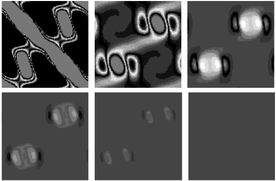
Figure 3: Frames of $U(u,v,\tau)$ for the polarized model $x=z=\Lambda=\sin u\sin v,\ p_{\Lambda}=12e^{\Lambda},\ \omega=r=0$. Time increases to the right and downward. The final frame corresponds to $U\approx 0$ everywhere.

The second model is unpolarized with $p$ given and the Hamiltonian constraint solved for $r$ in the IVP. Spatial averaging increases stability and allows the model to be followed to the point where only artifacts have $U\neq 0$ as is shown in Fig. 4. It certainly seems as if this model is also AVTD. Similar behavior is seen in other examples of this class.

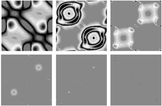
Figure 4: Frames of $U(u,v,\tau)$ for the generic model $x=z=\cos u\cos v,\ \Lambda=\sin u\sin v,\ p_{\Lambda}=14e^{\Lambda},\ p=10\cos u\cos v$ with averaging.

The last model has $r$ given with $p$ obtained by solving the Hamiltonian constraint in the IVP. Models of this type are less stable, probably due to the growth of a steep feature in $\omega$ which does not appear in the other cases. For this reason, the parameters must be kept small although the artifacts still appear more prominently. Fig. 5 shows that $U\to 0$ except near artifacts where no statement can be made.

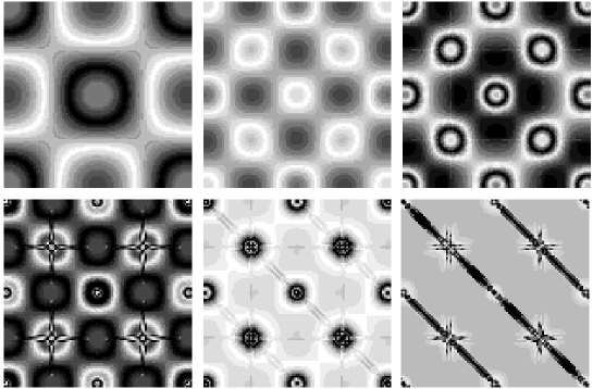
Figure 5: Frames of $U(u,v,\tau)$ for generic model $x=z=0,\ \Lambda=.1\cos u\cos v,\ p_{\Lambda}=2.1e^{\Lambda},\ r=\cos u\cos v$. The diagonal features in the final frames are numerical artifacts.

Thus, we may conclude that the application of the symplectic method to Einstein’s equations for collapsing universes allows the nature of the singularity to be studied. Application to the Gowdy model has yielded strong support for its conjectured AVTD singularity and has allowed the discovery and study of interesting small scale spatial structure and scaling. Further progress in understanding the generic singularity of $U(1)$ cosmologies requires imporvements in handling steep spatial gradients. (Spectral methods to evaluate spatial derivatives have been shown to work in the Gowdy simulations [80] and may yield improved behavior in the $U(1)$ case.) Nevertheless there is strong support that (at least within our restricted class of initial data) polarized models are AVTD. There is also support for AVTD behavior in all generic models studied so far. Mixmaster-like bounces have not been seen while $U$ appears to become small everywhere the results can be trusted. Several factors could account for this: (1) the BKL conjecture might be false; (2) the simulations have not run long enough; (3) Mixmaster behavior is present but hidden in our variables; or (4) our class of initial data is insufficiently generic. All these possibilities will be explored in studies in progress.

References

References

- [1] R.M. Wald, General Relativity, (University of Chicago, Chicago, 1984)
- [2] S.W. Hawking, Proc. Roy. Soc. Lond. A 300, 187 (1967).
- [3] S.W. Hawking, G.F.R. Ellis, The Large Scale Structure of Space-Time (Cambridge, Cambridge University, 1973).
- [4] S.W. Hawking, R. Penrose, Proc. Roy. Soc. Lond. A 314, 529 (1970).
- [5] D. Eardley, E. Liang, R. Sachs, J. Math. Phys. 13, 99 (1972).
- [6] J. Isenberg, V. Moncrief Ann. Phys. (N.Y.) 199, 84 (1990).
- [7] V.A. Belinskii, E.M. Lifshitz, I.M. Khalatnikov, Sov. Phys. Usp. 13, 745–765 (1971).
- [8] C.W. Misner, Phys. Rev. Lett. 22, 1071 (1969).
- [9] V. Moncrief, this volume.
- [10] A. Rendall, this volume.
- [11] L.S. Finn, this volume.
- [12] K.S. Thorne, in Magic without Magic, edited by J. Klauder (Freeman, San Francisco, 1974).
- [13] M. Choptuik, Phys. Rev. Lett. 70, 9 (1993)
- [14] S. Chandresekhar, J.B. Hartle, Proc. Roy. Soc. Lond. A384 301 (1982).
- [15] A.R. Moser, R.A. Matzner, M.P. Ryan, Jr., Ann. Phys. (N.Y.) 79, 558 (1973).
- [16] S.E. Rugh, B.J.T. Jones, Phys. Lett. A147, 353 (1990).
- [17] B.K. Berger, Phys. Rev. D 49, 1120 (1994).
- [18] G. Francisco, G.E.A. Matsas, J. Gen. Rel. Grav. 20, 1047 (1988).
- [19] A.B. Burd, N. Buric, G.F.R. Ellis, J. Gen. Rel. Grav. 22, 349 (1990).
- [20] D. Hobill, D. Bernstein, M. Welge, D. Simkins, Class. Quantum Grav. 8, 1155 (1991).
- [21] J. Pullin, in SILARG VII Relativity and Gravitation: Classical and Quantum, 1991.
- [22] J.D. Barrow, F. Tipler, Phys. Rep. 56, 372 (1979).
- [23] R. Penrose, Riv. Nuov. Cim. 1, 252 (1969).
- [24] S.L. Shapiro, S.A. Teukolsky, Phys. Rev. Lett. 66, 994 (1991).
- [25] T. Nakamura, H. Sato, Prog. Theor. Phys. 67, 1396 (1982).
- [26] E. Seidel, private communication
- [27] R.M. Wald, V. Iyer, Phys. Rev. D 44, 3719 (1991).
- [28] K.P. Tod, Class. Quantum Grav. 9, 1581 (1992).
- [29] S.L. Shapiro, S.A. Teukolsky, Phys. Rev. D 45, 2006 (1992).
- [30] S.L. Shapiro, S.A. Teukolsky, Astrophys. J. 419, 622 (1993).
- [31] F. Echeverria, Phys. Rev. D 47, 2271 (1993).
- [32] T. Chiba, T. Nakamura, K. Nakao, M. Sasaki, Class. Quantum Grav. 11, 431 (1994).
- [33] T. Nakamura, S.L. Shapiro, S.A. Teukolsky, Phys. Rev. D 38, 3972 (1988).
- [34] J. Wojtkiewicz, Phys. Rev. D 41, 1867 (1990).
- [35] C. Barrabès, W. Israel, P.S. Latlier, Phys. Lett. 160A, 41 (1991).
- [36] C. Barrabès, A. Gremain, E. Lesigne, P.S. Latlier, Class. Quantum Grav. 9, L105 (1992).
- [37] E.W. Hirschmann, D.M. Eardley, Phys. Rev. D 51, 4198 (1995).
- [38] A.M. Abrahams, C.R. Evans, Phys. Rev. Lett. 70, 2980 (1993).
- [39] D. Garfinkle, Phys. Rev. D 51, 5558 (1995).
- [40] D.S. Goldwirth, T. Piran, Phys. Rev. D 36, 3575 (1987).
- [41] D. Christodoulou, Comm. Math. Phys. 105, 337 (1986); 109, 613 (1987).
- [42] R.S. Hamadé, J.M. Stewart, gr-qc/9506044.
- [43] C.R. Evans and J.S. Coleman, Phys. Rev. Lett. 72, 1782 (1994).
- [44] E.W. Hirschmann, D.M. Eardley, gr-qc/9506078.
- [45] T. Koiki, T. Hara, S. Adachi, Phys. Rev. Lett. 74, 5170 (1995).
- [46] D. Maison, gr-qc/9504008.
- [47] C. Gundlach, Phys. Rev. Lett. 75, 3214 (1995).
- [48] E. Poisson, W. Israel, Phys. Rev. Lett. 63, 1663 (1989).
- [49] E. Poisson, W. Israel, Phys. Rev. D 41, 1796 (1990).
- [50] A. Ori, Phys. Rev. Lett. 67, 789 (1991).
- [51] A. Ori, Phys. Rev. Lett. 68, 2117 (1992).
- [52] M.L. Gnedin, N.Y. Gnedin, Class. Quantum Grav. 10, 1083 (1993).
- [53] P.R. Brady, J.D. Smith, Phys. Rev. Lett. 75, 1256 (1995).
- [54] A. Bonanno, S. Droz, W. Israel, S.M. Morsink, Proc. Roy. Soc. Lon. A 450, 553 (1995).
- [55] P. Hübner, gr-qc/940902.
- [56] H. Friedrich, Comm. Math. Phys. 119, 51 (1988).
- [57] D.F. Chernoff, J.D. Barrow, Phys. Rev. Lett. 50, 134 (1983).
- [58] J.D. Barrow, Phys. Rep. 85, 1 (1982).
- [59] I.M. Khalatnikov, E.M. Lifshitz, K.M. Khanin, L.N. Shchur, Ya.G. Sinai, J. Stat. Phys. 38, 97 (1985).
- [60] B.K. Berger, J. Gen. Rel. Grav. 23, 1385 (1991).
- [61] K. Ferraz, G. Francisco, G.E.A. Matsas, Phys. Lett. 156A, 407 (1991).
- [62] D. Hobill, A. Burd, A. Coley, editors, Deterministic Chaos in General Relativity (Plenum, New York, 1994).
- [63] V.G. LeBlanc, D. Kerr, J. Wainwright, Class. Quantum Grav. 12 513 (1995).
- [64] B.K. Berger, “Comment on the ‘Chaotic’ Singularity in Some Magnetic Bianchi VI0 Cosmologies,” submitted to Class. Quantum Grav.
- [65] R. Carretero-Gonzalez, H.N. Nunuz-Yepez, A.L. Salas-Brito, Phys. Lett. A188, 48 (1994).
- [66] S. Cotsakis, J. Demaret, Y. DeRop, L. Querella, Phys. Rev. D 48, 4595 (1993).
- [67] B.K. Berger, V. Moncrief, Phys. Rev. D 48, 4676 (1993).
- [68] B.K. Berger, D. Garfinkle, B. Grubis̆ić, V. Moncrief, “Phenomenology of the Gowdy Model on ,” unpublished.
- [69] G. Montani, Class. Quantum Grav. 12, 2505 (1995).
- [70] V.A. Belinskii, JETP Lett. 56, 421 (1992).
- [71] A.A. Kirillov, A.A. Kochnev, JETP Lett. 46, 435 (1987); A.A. Kirillov, JETP 76, 355 (1993).
- [72] V. Moncrief, Ann. Phys. (N.Y.) 167, 118 (1986).
- [73] R.H. Gowdy, Phys. Rev. Lett. 27 826 (1971).
- [74] B.K. Berger, Ann. Phys. (N.Y.) 83, 458 (1974).
- [75] B. Grubis̆ić, V. Moncrief, Phys. Rev. D 47 2371 (1993).
- [76] J.A. Fleck, J.R. Morris, M.D. Feit Appl. Phys. 10, 129 (1976).
- [77] V. Moncrief, Phys. Rev. D 28, 2485 (1983).
- [78] M. Suzuki, Phys. Lett. A146, 319 (1990).
- [79] B. Grubis̆ić, V. Moncrief, Phys. Rev. D 49, 2792 (1994).
- [80] B.K. Berger, “Application of a Spectral Symplectic Method to the Numerical Investigation of Cosmological Singularities,” unpublished.