Hyperfast interstellar travel in general relativity

Abstract

The problem is discussed of whether a traveller can reach a remote object and return back sooner than a photon would when taken into account that the traveller can partly control the geometry of his world. It is argued that under some reasonable assumptions in globally hyperbolic spacetimes the traveller cannot hasten reaching the destination. Nevertheless, it is perhaps possible for him to make an arbitrarily long round-trip within an arbitrarily short (from the point of view of a terrestrial observer) time.

1 Introduction

Everybody knows that nothing can move faster than light. The regrettable consequences of this fact are also well known. Most of the interesting or promising in possible colonization objects are so distant from us that the light barrier seems to make an insurmountable obstacle for any expedition. It is, for example, $200\,$pc from us to the Polar star, $500\,$pc to Deneb and $\sim 10\,$kpc to the centre of the Galaxy, not to mention other galaxies (hundreds of kiloparsecs). It makes no sense to send an expedition if we know that thousands of years will elapse before we receive its report. On the other hand, the prospects of being confined forever to the Solar system without any hope of visiting other civilizations or examining closely black holes, supergiants, and other marvels are so gloomy that it seems necessary to search for some way out.

In the present paper we consider this problem in the context of general relativity. Of course the light barrier exists here too. The point, however, is that in GR one can try to change the time necessary for some travel not only by varying one’s speed but also, as we shall show, by changing the distance one is to cover.

To put the question more specific, assume that we emit a beam of test particles from the Earth to Deneb (the event $S$). The particles move with all possible (sub)luminal speeds and by definition do not exert any effect on the surrounding world. The beam reaches Deneb (with the arrival time of the first particle $t_{\mathcal{D}}$ by Deneb’s clocks), reflects there from something, and returns to the Earth. Denote by $\Delta\tau_{\mathcal{E}}$ ($\tau_{\mathcal{E}}$ is the Earth’s proper time) the time interval between $S$ and the return of the first particle (the event $R$). The problem of interstellar travel lies just in the large typical $\Delta\tau_{\mathcal{E}}$. It is conceivable of course that a particle will meet a traversible wormhole leading to Deneb or an appropriate distortion of space shortening its way (see [2] and Example 4 below), but one cannot hope to meet such a convenient wormhole each time one wants to travel (unless one makes them oneself, which is impossible for the test particles). Suppose now that instead of emitting the test particles we launch a spaceship (i. e. something that does act on the surrounding space) in $S$. Then the question we discuss in this paper can be formulated as follows:

Is it possible that the spaceship will reach Deneb and then return to the Earth in $\Delta\tau^{\prime}<\Delta\tau_{\mathcal{E}}$?

By “possible” we mean “possible, at least in principle, from the causal point of view”. The use of tachyons, for example, enables, as is shown in [2], even a nontachionic spaceship to hasten its arrival. Suppose, however, that tachyons are forbidden (as well as all other means for changing the metric with violating what we call below “utter causality”). The main result of the paper is the demonstration of the fact that even under this condition the answer to the above question is positive. Moreover, in some cases (when global hyperbolicity is violated) even $t_{\mathcal{D}}$ can be lessened.

2 Causal changes

2.1 Changes of spacetime

In this section we make the question posed in the Introduction more concrete. As the point at issue is the effects caused by modifying the (four-dimensional) world (that is, by changing its metric or even topology), one may immediately ask, Modifying from what? To clarify this point first note that though we treat the geometry of the world classically throughout the paper (that is, we describe the world by a spacetime, i. e., by a smooth Lorentzian connected globally inextendible Hausdorff manifold), no special restrictions are imposed for a while on matter fields (and thus on the right-hand side of the Einstein equations). In particular, it is not implied that the matter fields (or particles) obey any specific classical differential equations.

Now consider an experiment with two possible results.

Example 1. A device set on a spaceship first polarizes an electron in the $y$-direction and then measures the $x$-component of its spin $\sigma_{x}$. If the result of the measurement is $\sigma_{x}=+1/2$, the device turns the spaceship to the right; otherwise it does not.

Example 2. A device set on a (very massive) spaceship tosses a coin. If it falls on the reverse the device turns the spaceship to the right; otherwise it does not.

Comment. One could argue that Example 2 is inadequate since (due to the classical nature of the experiment) there is actually one possible result in that experiment. That is indeed the case. However, let us

1. Assume that before being tossed the coin had never interacted with anything.

2. Neglect the contribution of the coin to the metric of the world.

Of course, items (i,ii) constitute an approximation and situations are conceivable for which such an approximation is invalid (e. g., item ($i$) can be illegal if the same coin was already used as a lot in another experiment involving large masses). We do not consider such situations. And if (i,ii) are adopted, experiment 2 can well be considered as an experiment with two possible results (the coin, in fact, is unobservable before the experiment).

Both situations described above suffer some lack of determinism (originating from the quantum indeterminism in the first case and from coarsening the classical description in the second). Namely, the spaceship is described now by a body whose evolution is not fixed uniquely by the initial data (in other words, its trajectory (non-analytic, though smooth) is no longer a solution of any “good” differential equation). However, as stated above, this does not matter much.

So, depending on which result is realized in the experiment (all other factors being the same; see below) our world must be described by one of two different spacetimes. It is the comparison between these two spacetimes that we are interested in.

Notation.

Let $M_{1}$ and $M_{2}$ be two spacetimes with a pair of inextendible timelike curves $\mathcal{E}_{i},{\mathcal{D}}_{i}\subset M_{i}\,$ in each (throughout the paper $i,j=1,2$). One of these spacetimes, $M_{1}$ say, is to describe our world under the assumption that we emit test particles at some moment $S_{1}\in\mathcal{E}_{1}$ and the other, under the assumption that instead of the particles we launch a spaceship in $S_{2}$, where $S_{2}\in M_{2}$ corresponds in a sense (see below) to $S_{1}$. The curves ${\mathcal{E}}_{i}$ and $\mathcal{D}_{i}$ are the world lines of Earth and Deneb, respectively. We require that the two pairs of points exist:

$$F_{i}\equiv\mbox{\rm Bd}\,\big{(}J^{+}(S_{i})\big{)}\cap{\mathcal{D}}_{i}\quad\mbox{and}\quad R_{i}\equiv\mbox{\rm Bd}\,\big{(}J^{+}(F_{i})\big{)}\cap{\mathcal{E}}_{i}.$$ (1)

These points mark the restrictions posed by the light barrier in each spacetime. Nothing moving with a subluminal speed in the world $M_{i}$ can reach Deneb sooner than in $F_{i}$ or return to the Earth sooner than in $R_{i}$. What we shall study is just the relative positions of $S_{i}\,,F_{i}\,,R_{i}$ for $i=1,2$ when the difference in the spacetimes $M_{1}$ and $M_{2}$ is of such a nature (below we formulate the necessary geometrical criterion) that it can be completely ascribed to the pilot’s activity after $S$.

2.2 “Utter causality”

The effect produced by the traveller on spacetime need not be weak. For example, by a (relatively) small expenditure of energy the spaceship can break the equilibrium in some close binary system on its way, thus provoking the collapse. The causal structures of $M_{1}$ and $M_{2}$ in such a case will differ radically. If an advanced civilization (to which it is usual to refer) will cope with topology changes, it may turn out that $M_{1}$ and $M_{2}$ are even nondiffeomorphic. So the spacetimes under discussion may differ considerably. On the other hand, we want them to be not too different:

1. The pilot of the spaceship deciding in $S$ whether or not to fly to Deneb knows the pilot’s past and in our model we would prefer that the pilot’s decision could not change this past. This restriction is not incompatible with the fact that the pilot can make different decisions (see the preceding subsection).

2. The absence of tachyons (i. e. fields violating the postulate of local causality [3]), does not mean by itself that one (located in, say, point $A$) cannot act on events lying off one’s “causal future” (i. e. off $J^{+}(A)$).

• Matter fields are conceivable that while satisfying local causality themselves do not provide local causality to the metric. In other words, they afford a unique solution to the Cauchy problem for the metric, not in $D^{+}({\cal P})$ (cf. chapter 7 in [3]), but in some smaller region only. In the presence of such fields the metric at a point $B$ might depend on the fields at points outside $J^{-}(B)$. That is, the metric itself would act as a tachyon field in such a case.

• Let $M_{1}$ be the Minkowski space with coordinates $(t_{1},x_{1}^{\mu})$ and $M_{2}$ be a spacetime with coordinates $(t_{2},x_{2}^{\mu})$ and with the metric flat at the region $x^{1}_{2}>t_{2}$, but nonflat otherwise (such a spacetime describes, for example, propagation of a plane electromagnetic wave). Intuition suggests that the difference between $M_{1}$ and $M_{2}$ is not accountable to the activity of an observer located in the origin of the coordinates, but neither local causality nor any other principle of general relativity forbids such an interpretation.

In the model we construct we want to abandon any possibility of such “acausal” action on the metric. In other words, we want the condition relating $M_{1}$ and $M_{2}$ to imply that these worlds are the same in events that cannot be causally connected to $S$. This requirement can be called the principle of utter causality.

2.3 Relating condition

In this section we formulate the condition relating $M_{1}$ to $M_{2}$. Namely, we require that $M_{i}$ should “diverge by $S$” (see below). It should be stressed that from the logical point of view this condition is just a physical postulate. Being concerned only with the relation between two “possible” worlds, this new postulate does not affect any previously known results. In defense of restrictions imposed by our postulate on $M_{i}$ we can say that it does not contradict any known facts. Moreover, in the absence of tachyons (in the broad sense, see item (i) above) it is hard to conceive of a mechanism violating it.

Formulating the condition under discussion we would like to base it on the “principle of utter causality”. In doing so, however, we meet a circle: to find out whether a point is causally connected to $S_{i}$ we must know the metric of the spacetime $M_{i}$, while the metric at a point depends in its turn on whether or not the point can be causally connected to $S_{i}$. That is why we cannot simply require that $M_{i}\setminus J^{+}(S_{i})$ be isometric. The following example shows that this may not be the case even when utter causality apparently holds.

Example 3. “Hyper-jump.”

Let $M_{1}$ be the Minkowski plane with $S_{1}$ located at the origin of the coordinates and let $M_{2}$ be the spacetime (similar to the Deutsch-Politzer space) obtained from $M_{1}$ by the following procedure (see Fig. 1). Two cuts are made, one along a segment $l$ lying in $I^{+}(S_{1})$ and another along a segment $l^{\prime}$ lying off $J^{+}(S_{1})$ and obtained from $l$ by a translation. The four points bounding $l,\,l^{\prime}$ are removed and the lower (or the left, if $l$ is vertical) bank of each cut is glued to the upper (or to the right) bank of the other. Note that we can vary the metric in the shadowed region without violating utter causality though this region “corresponds” to a part of $M_{1}\setminus J^{+}(S_{1})$.

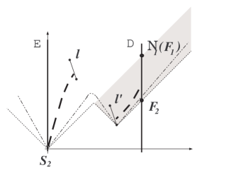
Figure 1: “Hyper-jump.” The thick dashed line depicts an allowed world line of a spaceship.

To overcome this circle we shall formulate our relating condition in terms of the boundaries of the “unchanged” regions.

Notation.

Below we deal with two spacetimes $N_{i}\subset M_{i}$ related by an isometry $\phi\colon\;N_{2}=\phi(N_{1})$. To shorten notation we shall write sometimes $X_{(1)}$ for a subset $X\subset N_{1}$, and $X_{(2)}$ for $\phi(X)$. The notation $A\;{\star}\;B$ for points $A,\,B$ will mean that there exists a sequence $\{a_{n}\}$:

$$a_{n(i)}\to A,\quad a_{n(j)}\to B.$$

Clearly if $A\in N_{1}$, then $A\;{\star}\;B\neq A$ means simply $B=\phi(A)$. Lastly, $\vphantom{\bigg{|}}\mathbb{J}\equiv\overline{J^{+}(S_{1})}\cup\overline{J^{+}(S_{2})}$.

Definition 1.

We call spacetimes $M_{1},\>M_{2}$ diverging by the event $S_{1}$ (or by $S_{2}$, or simply by $S$) if there exist open sets $N_{i}\subset M_{i}$, points $S_{i}$, and an isometry $\phi\colon\;N_{1}\mapsto N_{2}$ such that $I^{-}(S_{2})=\phi\big{(}I^{-}(S_{1})\big{)}$ and

$$(Q_{j}\cup Q_{k})\cap{\mathbb{J}}\neq\emptyset$$ (2)

whenever $Q_{j}\in\mbox{\rm Bd}\,N_{j}$ and $Q_{j}\;{\star}\;Q_{k}\neq Q_{j}$.

Comment.

In the example considered above the two spacetimes diverged by $S$. Note that
(i) The possible choice of $N_{i}$ is not unique. The dotted lines in Fig. 1 bound from above two different regions that can be chosen as $N_{2}$.
(ii) $A_{(2)}\prec B_{(2)}$ does not necessarily imply ${}_{(1)}\prec B_{(1)}$. (iii) Points constituting the boundary of $N$ fall into two types, some have counterparts (i. e. points related to them by $\star$) in the other spacetime and the others do not (corresponding thus to singularities). It can be shown (see Lemma 1 in the Appendix) that the first type points form a dense subset of $\mbox{\rm Bd}\,N$.

In what follows we proceed from the assumption that the condition relating the two worlds is just that they are described by spacetimes diverging by $S$ (with $N_{i}$ corresponding to the unchanged regions). It should be noted, however, that this condition is tentative to some extent. It is not impossible that some other conditions may be of interest, more restrictive than ours (e. g. we could put some requirements on points of the second type) or, on the contrary, less restrictive. The latter can be obtained, for example, in the following manner. The relation $\star$ is reflective and symmetric, but not transitive. Denote by $\sim$ its transitive closure (e. g. in the case depicted in Fig. 2, $A\;\hbox to0.0pt{$\displaystyle\hbox to5.16663pt{\hfill/}$\hss}{\star}\;B$, but $A\sim B$).

Figure 2: Make cuts along the thin lines on the cylinder at the left and glue their banks to obtain the “trousers” at the right. The shadowed regions depict $J^{+}(S)$. Note that these spacetimes cannot be considered as diverging by $S$. For, if we take, for example, the whole $M_{i}$ with the thin lines removed, as $N_{i}$, then $\mbox{\rm Bd}\,N_{1}\ni B\;{\star}\;C$, while neither $B$ nor $C$ lies in $\mathbb{J}$.

Now, if we want to consider topology changes like that in Fig. 2 as possibly produced by the event $S$, we can replace (2) by the requirement that for any first type point $Q\in\mbox{\rm Bd}\,N_{j}$,

$$[Q]_{\sim}\cap\mathbb{J}\neq\emptyset,$$ (3)

where $[Q]_{\sim}\equiv\{x{|}\;x\sim Q\}$. It is worth pointing out that replacing (2) by (3) does not actually affect any of the statements below.

Now we can formulate the question posed in the Introduction as follows:

Given that spacetimes $M_{i}$ diverged by an event $S$, how will the points $F_{2},\>R_{2}$ be related to the points $F_{1},\>R_{1}$?

(It is understood from now on that

$$\mathcal{C}_{2}\cap N_{2}=\phi(\mathcal{C}_{1}\cap N_{1}),$$

where $\mathcal{C}_{i}=\mathcal{D}_{i},\,\mathcal{E}_{i}$.)

3 One-way trip

Example 3 shows that contrary to what one might expect, utter causality by itself does not prevent a pilot from hastening the arrival at a destination. It is reasonable to suppose, however, that in less “pathological” spacetimes this is not the case.

Proposition 1.

If $M_{i}$ are globally hyperbolic spacetimes diverging by $S$, then

$$F_{1}\;{\star}\;F_{2}.$$

The proof of this seemingly self-evident proposition has turned out to be quite tedious, so we cite it in the Appendix.

Example 4.

Recently it was proposed [2] to use for hyper-fast travel the metric (I omit two irrelevant dimensions $y$ and $z$)

$$ds^{2}=-dt^{2}+[dx-v_{s}f(r_{s})dt]^{2}.$$ (4)

Here $r_{s}\equiv|x-x_{s}|,\ v_{s}(t)\equiv dx_{s}(t)/dt$, and $x_{s}(t)$ and $f$ are arbitrary smooth functions satisfying

$$x_{s}(t)=\cases{D&at $t>T$\cr 0&at $t<0$\cr}\qquad f(\xi)=\cases{1&for $\xi\in(-R+\delta,R-\delta)$\cr 0&for $\xi\notin(-R,R)$.\cr}$$

$\delta,\ T$, and $R$ are arbitrary positive parameters.

To see the physical meaning of the condition of utter causality take the Minkowski plane as $M_{1}$ and the plane endowed with the metric (4) as $M_{2}$ (the $S_{i}$ are meant to be the origins of the coordinates). It is easy to see that the curve $\lambda\equiv(t,x_{s}(t))$ is timelike with respect to the metric (4) for any $x_{s}(t)$. So we could conclude that an astronaut can travel with an arbitrary velocity (“velocity” here is taken to mean the coordinate velocity $dx_{a}(t)/dt$, where $x_{a}(t)$ is the astronaut’s world line). All he needs is to choose an appropriate $x_{a}(t)$ and to make the metric be of form (4) with $x_{s}(t)=x_{a}(t)$. The distortion of the spacetime in the region $\{0<x<D,\ t>0\}$ of $M_{2}$ will allow him to travel faster than he could have done in the flat space $M_{1}$ (which does not of course contradict the Proposition since the $M_{i}$ do not diverge by $S$).

The subtlety lies in the words “to make the metric be ….” Consider the curve $\lambda_{+}\equiv(t,x_{s}(t)+R)$, which separates the flat and the curved regions. It is easy to see that $v_{s}(t)>1$ when and only when $\lambda_{+}(t)$ is spacelike. At the same time eq. (19) of [2] says that the space immediately to the left of $\lambda_{+}$ is filled with some matter ($G^{00}\neq 0$). The curve $\lambda_{+}(t)$ is thus the world line of the leading edge of this matter. We come therefore to the conclusion that to achieve $T<D$ the astronaut has to use tachyons. This possibility is not too interesting: no wonder that one can overcome the light barrier if one can use the tachyonic matter. Alternatively, in the more general case, when the spacetime is nonflat from the outset, a similar result could be achieved without tachyons by placing in advance some devices along the pilot’s way and programming them to come into operation at preassigned moments and to operate in a preassigned manner. Take the moment $P$ when we began placing the devices as a point diverging the spacetimes. Proposition 1 shows then that, though a regular spaceship service perhaps can be set up by this means, it does not help to outdistance the test particles from $M_{1}$ in the first flight (i. e. in the flight that would start at $P$).

4 Round-trip

The situation with the points $R_{i}$ differs radically from that with $F_{i}$ since the segment $FR\,$ belongs to $J^{+}(S)$ for sure. So even in globally hyperbolic spacetimes there is nothing to prevent an astronaut from modifying the metric so as to move $R$ closer to $S$ (note that from the viewpoint of possible applications to interstellar expeditions this is far more important than to shift $F$). Let us consider two examples.

Example 5. “The warp drive.”

Consider the metric

$$ds^{2}=-(dt-dx)(dt+k(t,x)dx),$$

where $k\equiv 1-(2-\delta)\theta_{\epsilon}(t-x)[\theta_{\epsilon}(x)-\theta_{\epsilon}(x+\epsilon-D)]$. Here $\theta_{\epsilon}$ denotes a smooth monotone function:

$$\theta_{\epsilon}(\xi)=\cases{1&at $\xi>\epsilon$\cr 0&at $\xi<0$\cr}$$

$\delta$ and $\epsilon<D$ being arbitrary small positive parameters.

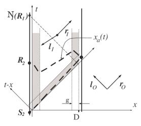
Figure 3: Warp drive.

Three regions can be recognized in $M$ (see Fig. 3):

The outside region: $\{x<0\}\cup\{x>D\}\cup\{x>t\}.$ The metric is flat here ($k=1$). Future light cones are generated by vectors $\mathbf{r}_{O}=\partial_{t}+\partial_{x}$ and $\mathbf{l}_{O}=\partial_{t}-\partial_{x}$
The transition region. It is a narrow (of width $\sim\epsilon$) strip shown as a shaded region in Fig. 3. The spacetime is curved here.
The inside region: $\{x<t-\epsilon\}\cap\{\epsilon<x<D-\epsilon\}.$ This region is also flat ($k=\delta-1$), but the light cones are “more open” here being generated by ${\mathbf{r}}_{I}=\partial_{t}+\partial_{x}$ and ${\mathbf{l}}_{I}=-(1-\delta)\partial_{t}-\partial_{x}$.

The vector ${\mathbf{l}}_{I}$ is almost antiparallel to ${\mathbf{r}}_{I}$ and thus a photon moving from $F$ toward the left will reach the line $x=0$ almost in $S$.

We see thus that an arbitrarily distant journey can be made in an arbitrarily short time! It can look like the following. In 2000, say, an astronaut — his world line is shown as a bold dashed line in Fig. 3 — starts to Deneb. He moves with a near light speed and the way to Deneb takes the (proper) time $\Delta\tau_{a}\ll 1600\,$yr for him. On the way he carries out some manipulations with the ballast or with the passing matter. In spite of these manipulations the traveller reaches Deneb at 3600 only. However, on his way back he finds that the metric has changed and he moves “backward in time,” that is, $t$ decreases as he approaches the Earth (though his trajectory, of course, is future-directed). As a result, he returns to the Earth in 2002.

Example 6. Wormhole.

Yet another way to return arbitrarily soon after the start by changing geometry is the use of wormholes. Assume that we have a wormhole with a negligibly short throat and with both mouths resting near the Earth. Assume further that we can move any mouth at will without changing the “inner” geometry of the wormhole. Let the astronaut take one of the mouths with him. If he moves with a near light speed, the trip will take only the short time $\Delta\tau_{a}$ for him. According to our assumptions the clocks on the Earth as seen through the throat will remain synchronized with his and the throat will remain negligibly short. So, if immediately after reaching Deneb he returns to the Earth through the wormhole’s throat, it will turn out that he will have returned within $\Delta\tau_{\mathcal{E}}\approx\Delta\tau_{a}$ after the start.

Similar things were discussed many times in connection with the wormhole-based time machine. The main technical difference between a time machine and a vehicle under consideration is that in the latter case the mouth only moves away from the Earth. So causality is preserved and no difficulties arise connected with its violation.

5 Discussion

In all examples considered above the pilot, roughly speaking, “transforms” an “initially” spacelike (or even past-directed) curve into future-directed. Assume now that one applies this procedure first to a spacelike curve $(AC_{1}B)$ and then to another spacelike curve $(BC_{2}A)$ lying in the intact until then region. As a result one obtains a closed timelike curve $(AC_{1}BC_{2}A)$ (see [5, 6, 7] for more details). So the vehicles in discussion can be in a sense considered as “square roots” of time machine (and thus a collective name space machine — also borrowed from science fiction — seems most appropriate for them). The connection between time and space machines allows us to classify the latter under two types.
1. Those leading to time machines with compactly generated Cauchy horizons (Examples 4–6). From the results of [8] it is clear that the creation of a space machine of this type requires violation of the weak energy condition. The possibility of such violations is restricted by the so-called “quantum inequalities”, QIs [9]. In particular, with the use of a QI it was shown in [6] that to create a four-dimensional analog of our Example 5 one needs huge amounts (e. g. $10^{32}M_{galaxy}$) of “negative energy”. Thermodynamical considerations suggest that this in its turn necessitates huge amounts of “usual” energy, which makes the creation unlikely. This conclusion is quite sensitive to the details of the geometry of the space machine and one could try to modify its construction so as to obtain more appropriate values. Another way, however, seems more promising. The QI used in [6] was derived with the constraint (see [9]) that in a region with the radius smaller than the proper radius of curvature spacetime is “approximately Minkowski” in the sense that the energy density (to be more precise, the integral $E[\lambda,\tau_{0},T]\equiv\int_{-\infty}^{T}\langle T_{\mu\nu}u^{\mu}u^{\nu}\rangle({\tau}^{2}+{\tau_{0}}^{2})^{-1}\,d\tau$, where $\lambda$ is a timelike geodesic parametrized by the proper time $\tau$, $\mathbf{u}\equiv\partial_{\tau}$, and $\tau_{0}$ is a “sampling time”) is given by essentially the same expression as in the Minkowski space. So, in designing space machines, spacetimes are worth searching for where this constraint breaks down.

Among them is a “critical” (i. e. just before its transformation into a time machine) wormhole. Particles propagating through such a wormhole again and again experience (regardless of specific properties of the wormhole [10]) an increasing blueshift. The terms in the stress-energy tensor associated with nontrivial topology also experience this blue-shift [11]. As a result, in the vicinity of the Cauchy horizon (even when a region we consider is flat and is located far from either mouth) the behaviour of the energy density has nothing to do with what one could expect from the “almost Minkowski” approximation [12]. (The difference is so great that beyond the horizon we cannot use the known quantum field theory, including its methods of evaluating the energy density, at all [13].) Consider, for example, the Misner space with the massless scalar field in the conformal vacuum state. From the results of Sec. III.B [12] it is easy to see that $E[\lambda,\tau_{0},\infty]=-\infty$ for any $\lambda$ and $\tau_{0}$ and the QI thus does not hold here. Moreover, $E[\lambda,\tau_{0},T]\to-\infty$ as one approaches the Cauchy horizon along $\lambda$. So, we need not actually create a time machine to violate the QI. It would suffice to “almost create” it.

Thus it well may be that in spite of (or owing to) the use of a wormhole the space machine considered in Example 6 will turn out to be more realistic than that in Example 5.

2. Noncompact space machines, as in Example 3. These (even their singularity free versions; see [4, 14]) do not necessitate violations of the weak energy condition. They have, however, another drawback typical for time machines. The evolution of nonglobally hyperbolic spacetimes is not understood clearly enough and so we do not know how to force a spacetime to evolve in the appropriate way. There is an example, however (the wormhole-based time machine [15]), where the spacetime is denuded of its global hyperbolicity by quite conceivable manipulations, which gives us some hope that this drawback is actually not fatal.

Appendix

Throughout this section we take $M_{i}$ to be globally hyperbolic spacetimes diverging by $S$ and $(U)_{\mathbb{J}}$ to mean $U\setminus\mathbb{J}$ for any set $U$.

Lemma 1.

Let $O$ be a neighbourhood of a point of $\mbox{\rm Bd}\,N_{j}$ and ${O^{N}}\subset O\cap N_{j}$ be such an open nonempty set that

$$\mbox{\rm Bd}\,{O^{N}}\cap O\subset\mbox{\rm Bd}\,N_{j}$$ (5)

Then

$$\mbox{\rm Bd}\,{O^{N}}_{(i)}\cap J^{+}(S_{i})\neq\emptyset\qquad\mbox{for some }i.$$

Proof.

Let $j=1$ for definiteness. Consider a smooth manifold $\widetilde{M}\equiv M_{2}\cup_{\phi^{\prime}}O$, where ${\phi^{\prime}}$ is the restriction of ${\phi}$ on ${O^{N}}$. Induce the metric on $\widetilde{M}$ by the natural projections

$$\pi_{i}\colon\qquad M_{2}\stackrel{{\scriptstyle\pi_{1}}}{{\longmapsto}}\widetilde{M},\quad O\stackrel{{\scriptstyle\pi_{2}}}{{\longmapsto}}\widetilde{M}$$

(or, more precisely by $\pi_{i}^{-1}$) thus making $\widetilde{M}$ into a Lorentzian manifold and $\pi_{i}$ into isometrical embeddings. $\widetilde{M}$ must be non-Hausdorff since otherwise it would be a spacetime and so (as $M_{2}\varsubsetneq\widetilde{M}$) $M_{2}$ would have an extension in contradiction to its definition. So points $Q_{i}$ exist:

$$Q_{1}\;{\star}\;Q_{2},\qquad Q_{1}\in\mbox{\rm Bd}\,{O^{N}}_{(1)}\cap O,\quad Q_{2}\in\mbox{\rm Bd}\,{O^{N}}_{(2)}$$ (6)

and the lemma follows now from Def. 1 coupled with (5).

$\square$

Lemma 2.

If both $A_{(i)}$ lie in $(N_{i})_{\mathbb{J}}$, then so do $I^{-}(A_{(i)})$.

Proof.

$M_{i}$ are globally hyperbolic. So any point $P$ has such a neighbourhood (we shall denote it by $V_{P}$) that, first, it is causally convex, i. e.  $J^{-}(x)\cap J^{+}(y)\subset V_{P}$ for any points $x,\,y\colon\;y\in J^{-}(x,V_{P})$; and, second, it lies in a convex normal neighbourhood of $P$. Now suppose the lemma were false. We could find then such a point $A^{\prime}\in I^{-}(A_{(i)},N_{i})$ (let $i=1$, for definiteness) that

$$W\neq I^{-}(A^{\prime},V_{A^{\prime}}),$$

where $W\equiv I^{-}(A^{\prime},N_{1}\cap V_{A^{\prime}})$.

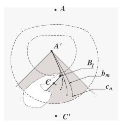
Figure 4: Case 1 of Lemma 2. The white area does not belong to $N_{1}$, the darkest area is $W$. If instead of the larger area bounded by a dashed line we take the smaller one as $V_{A^{\prime}}$, we get Case 2.

Denote $\mbox{\rm Bd}\,W\cap I^{-}(A^{\prime},V_{A^{\prime}})$ by $\partial W$. Clearly $\emptyset\neq\partial W\subset\overline{N_{1}}$. So, let us consider the two possible cases (see Fig. 4):
I. $\partial W\not\subset\mbox{\rm Bd}\,N_{1}$.
Under this condition a point $C$ and a sequence of causal curves $\{\gamma_{n}\}$ from $A^{\prime}$ to points $c_{n}$ exist such that

$$\gamma_{n}\subset W,\quad c_{n}\to C\in\partial W\cap N_{1}$$

According to [16, Prop. 2.19] there exists a causal curve $\gamma$ connecting $A^{\prime}$ and $C$, which is limit for $\{\gamma_{n}\}$ and is lying thus in $\overline{W}$. Since $V_{A^{\prime}}$ belongs to a normal convex neighbourhood and $C\in I^{-}(A^{\prime},V_{A^{\prime}})$, $\gamma$ by [3, Prop. 4.5.1] is not a null geodesic and hence

$$\gamma\not\subset N_{1}$$ (7)

(otherwise by [3, Prop. 4.5.10] and by causal convexity of $V_{A^{\prime}}$ we could deform it into a timelike curve lying in $N_{1}\cap V_{A^{\prime}}$, while $C\notin W$).

Now note that for any $C^{\prime}\in I^{-}(C,N_{1})$ there exists a subsequence $\{\gamma_{k}\}$ lying in $I^{+}(C^{\prime},N_{1})$. So by (7) a sequence of points $\{b_{m}\}$ and a point $B_{1}$ can be found such that

$$b_{m}\to B_{1}\in\mbox{\rm Bd}\,N_{1},\qquad b_{m}\in I^{-}(A^{\prime},N_{1})\cap I^{+}(C^{\prime},N_{1}).$$ (8)

Thus the $\phi(b_{m})$ lie in a compact set $J^{-}(A^{\prime}_{(2)})\cap J^{+}(C^{\prime}_{(2)})$ and therefore

$$\phi(b_{m})\to B_{2}\colon\quad B_{1}\;{\star}\;B_{2}.$$

From Def. 1 it follows that at least one of the $B_{i}$ lies in $J^{+}(S_{i})$ and since $B_{i}\in I^{-}(A_{(i)})$ we arrive at a contradiction.
II. $\partial W\subset\mbox{\rm Bd}\,N_{1}$.
In this case taking $O=I^{-}(A^{\prime},V_{A^{\prime}})$ and ${O^{N}}=W$ in Lemma 1 yields

$$\overline{W_{(i)}}\cap J^{+}(S_{i})\neq\emptyset\qquad\mbox{for some }i,$$

which gives a contradiction again since $\overline{W_{(i)}}\subset I^{-}(A_{(i)})$.

$\square$

Consider now the sets $L_{i}\equiv\{x|\;I^{-}(x)\subset N_{i}\}$. They have a few obvious features:

$$L_{i}=\overline{\mbox{\rm Int}\,L_{i}},\quad\mbox{\rm Int}\,L_{i}\subset N_{i}$$ (9)

$$A_{(1)}\in(L_{1})_{\mathbb{J}}\quad\Leftrightarrow\quad A_{(2)}\in(L_{2})_{\mathbb{J}}$$ (10)

Combining Lemma 2 with (9,10) we obtain:

$$(\mbox{\rm Bd}\,L_{i})_{\mathbb{J}}\subset\mbox{\rm Bd}\,N_{i}.$$ (11)

Lemma 3.

$(L_{i})_{\mathbb{J}}=(M_{i})_{\mathbb{J}}$.

Proof.

Since $(M_{i})_{\mathbb{J}}$ is connected and $(\mbox{\rm Int}\,L_{i})_{\mathbb{J}}$ is non-empty [e. g. from Def. 1 $I^{-}(S_{i})\subset(\mbox{\rm Int}\,L_{i})_{\mathbb{J}}$] it clearly suffices to prove that $(\mbox{\rm Bd}\,L_{i})_{\mathbb{J}}=\emptyset$. To obtain a contradiction, suppose that there exists a point $A\in(\mbox{\rm Bd}\,L_{1})_{\mathbb{J}}$ and let $U$ be such a neighbourhood of $A$ that

$$\overline{U}\subset(M_{1})_{\mathbb{J}}$$

Then for ${U^{L}}\equiv U\cap\mbox{\rm Int}\,L_{1}$ it holds that

$$\overline{{U^{L}}_{(i)}}\cap J^{+}(S_{i})=\emptyset\qquad i=1,2.$$

On the other hand, owing to (9,11) we can take $O=U$ and ${O^{N}}={U^{L}}$ in Lemma 1 and get

$$\overline{{U^{L}}_{(i)}}\cap J^{+}(S_{i})\neq\emptyset\qquad\mbox{for some }i.$$

Contradiction.

$\square$

Corollary 1.

$(I^{+}(\mathcal{E}_{2}))_{\mathbb{J}}=\phi\big{(}(I^{+}(\mathcal{E}_{1}))_{\mathbb{J}}\big{)}$.

Proof of Proposition 1.

$M_{i}$ is causally simple. Hence a segment of null geodesic from $S_{i}$ to $F_{i}$ exists. By [3, Prop. 4.5.10] this implies that any point $P_{(i)}\in(\mathcal{E}_{i})_{\mathbb{J}}$ can be connected to $F_{i}$ by a timelike curve. Hence a point $P^{\prime}\in(\mathcal{D}_{i})_{\mathbb{J}}$ can be reached from $P_{(i)}$ by a timelike curve without intersecting $J^{+}(S_{i})$. Thus $F_{i}$ is the future end point of the curve $\mathcal{D}^{\prime}_{i}$:

$$\mathcal{D}^{\prime}_{i}\equiv\mathcal{D}\cap(I^{+}(\mathcal{E}_{i}))_{\mathbb{J}}$$

And from Corollary 1 it follows that $\phi(\mathcal{D}^{\prime}_{1})=\mathcal{D}^{\prime}_{2}$.

$\square$

References

- [1] S. Lem 1989 Return from the stars (Harcourt, Brace and Co.)
- [2] M. Alcubierre, Class. Quantum Grav. 11, L73 (1994)
- [3] S. W. Hawking and G. F. R. Ellis 1973 The Large Scale Structure of Spacetime (Cambridge, Cambridge University Press)
- [4] S. V. Krasnikov gr-qc 9702031
- [5] A. Everett, Phys. Rev. D 53, 7365 (1996)
- [6] A. E. Everett and T. A. Roman, Phys. Rev. D 56, 2100 (1997)
- [7] M. S. Morris and K. S. Thorne, Am. J. Phys. 56, 395 (1988)
- [8] S. W. Hawking, Phys. Rev. D 46, 603 (1992)
- [9] L. H. Ford and T. A. Roman, Phys. Rev. D 53, 5496 (1996)
- [10] S. V. Krasnikov, Class. and Quantum Grav. 11, 1 (1994)
- [11] U. Yurtsever, Class. Quantum Grav. 8, 1127 (1991)
- [12] S. V. Krasnikov, Phys. Rev. D 54, 7322 (1996)
- [13] B. S. Kay, M. J. Radzikowski, and R. M. Wald, Commun. Math. Phys. 183, 533 (1997); S. V. Krasnikov gr-qc 9802008
- [14] S. V. Krasnikov, Gen. Relativ. Gravit. 27, 529 (1995)
- [15] M. S. Morris, K. S. Thorne, and U. Yurtsever, Phys. Rev. Lett. 61, 1446 (1988)
- [16] J. Beem and P. Ehrich 1981 Global Lorentzian Geometry (N. Y., Marcel Dekker. Ink.)