LONG RANGE EFFECTS
OF COSMIC STRING STRUCTURE

Abstract

We combine and further develop ideas and techniques of Allen & Ottewill, Phys. Rev. D, 42, 2669 (1990) and Kay & Studer Commun. Math. Phys., 139, 103 (1991) for calculating the long range effects of cosmic string cores on classical and quantum field quantities far from an (infinitely long, straight) cosmic string. We find analytical approximations for (a) the gravity-induced ground state renormalized expectation values of $\hat{\varphi}^{2}$ and $\hat{T}_{\mu}{}^{\nu}$ for a non-minimally coupled quantum scalar field far from a cosmic string (b) the classical electrostatic self force on a test charge far from a superconducting cosmic string. Surprisingly – even at cosmologically large distances – all these quantities would be very badly approximated by idealizing the string as having zero thickness and imposing regular boundary conditions; instead they are well approximated by suitably fitted strengths of logarithmic divergence at the string core. Our formula for ${\langle{\hat{\varphi}}^{2}\rangle}$ reproduces (with much less effort and much more generality) the earlier numerical results of Allen & Ottewill. Both ${\langle{\hat{\varphi}}^{2}\rangle}$ and ${\langle{\hat{T}}_{\mu}{}^{\nu}\rangle}$ turn out to be “weak field topological invariants” depending on the details of the string core only through the minimal coupling parameter “$\xi$” (and the deficit angle). Our formula for the self-force (leaving aside relatively tiny gravitational corrections) turns out to be attractive: We obtain, for the self-potential of a test charge $Q$ a distance $r$ from a (GUT scale) superconducting string, the formula $-Q^{2}/(16\epsilon_{0}r\ln(qr))$ where $q$ is an (in principle, computable) constant of the order of the inverse string radius.

I INTRODUCTION

A realistic cosmic string has structure on a length scale defined by the phase transition at which it is formed. In the case of a GUT string this corresponds to a radius of order $10^{-30}\,$cm. As this radius is so small, one often models the true string space-time by an idealized space-time where the string core has zero thickness and the curvature is represented by a 2-dimensional delta-function. The idealized model for an infinitely long straight static cosmic string space-time is the manifold $R^{2}\times R^{+}\times S^{1}$ with conical metric

$${\rm d}s^{2}=-{\rm d}t^{2}+{\rm d}z^{2}+{\rm d}r^{2}+r^{2}{\rm d}\phi^{2}\quad,$$ (1)

where the angular range is $\phi\in[0,2\pi/\kappa)$, corresponding to a deficit angle of $2\pi(1-1/\kappa)$. Throughout this paper we shall assume the standard case of positive deficit angle, so that $\kappa>1$; for GUT strings $\kappa-1\sim 10^{-6}$.

In studying the behaviour of various types of fields and waves far from such a string, it is sometimes erroneously taken for granted that one can always ignore the details of the interior structure of the string and approximate the effect of the string by this idealized model with regularity conditions placed at the conical singularity. This paper presents two calculations involving fields propagating around and interacting with a cosmic string for which this is not true. These calculations have, instead, the remarkable feature that the quantity calculated, even at very large distances from the string, depends on details of the interaction inside the string core.

We shall start by treating a ‘realistic’ or ‘true’ cosmic string having a core of finite thickness with a definite radius $a$ (but assumed for simplicity to be infinitely long, straight and static). This corresponds to a space-time metric taking the standard conical form with given deficit angle outside the radius $a$, but matching onto a smooth model core metric inside this radius (see Eq. (4) below).

The first calculation involves a non-minimally coupled quantum linear scalar field $\hat{\varphi}(x)$: We shall obtain an approximate formula for the renormalized vacuum expectation value ${\langle{\hat{\varphi}}^{2}\rangle}$ for such a field far from the string and a similar formula for the expectation value of the energy-momentum tensor ${\langle{\hat{T}}_{\mu}{}^{\nu}\rangle}$. The second calculation concerns a classical electrostatic field at large distances from a superconducting cosmic string: In this case the string is additionally characterized by a non-vanishing function within the core representing the ‘local photon mass term’ responsible for making it superconducting [1]. We shall obtain an approximate formula for the self-force on a test charge far from the string due to the presence of such a string. (As we shall see, this self-force arises as the sum of two terms: A small repulsive term previously calculated by Smith [2] and Linet [3] which depends on the deficit angle and a typically much larger attractive term which depends on the “scattering length” of the local photon mass term and is independent of the deficit angle.)

Both calculations presented here involve calculating Green functions $G$ for equations of the schematic form

$$(-\Delta+V)G=\delta$$ (2)

and both involve calculating (suitably renormalized) coincident-point values of such Green functions. In the calculation of ${\langle{\hat{\varphi}}^{2}\rangle}$, $\Delta$ represents the Laplace-Beltrami operator for the (Euclideanized) 4-dimensional string space-time metric, while $V$ represents a non-minimal coupling term $\xi{\cal R}$, where $\cal R$ is the Ricci scalar of the same metric. In the calculation of the self-force, $\Delta$ represents the Laplace-Beltrami operator for the 3-dimensional spatial metric of the string at a fixed time while $V$ represents the local photon mass term regarded as a function on that 3-dimensional space. For both calculations presented here, the sensitivity to the core structure can be traced back to the potential term $V$ in Eq. (2). For example, in the case of the calculation of ${\langle{\hat{\varphi}}^{2}\rangle}$ for a minimally coupled quantum scalar field (corresponding to $V=0$), one can idealize the true space-time of the cosmic string by the idealized conical space-time (1) and, with the imposition of regularity conditions on the scalar field at the conical singularity, obtain an excellent approximation to ${\langle{\hat{\varphi}}^{2}\rangle}$ at large distances from the string (seeSec. IV).

That the value of ${\langle{\hat{\varphi}}^{2}\rangle}$ for a non-minimally coupled field will depend on the details of the metric in the core of the string even very far from the string was argued by Allen and Ottewill in [4]. There the argument was confirmed by detailed calculations for two model cores: the ‘flower pot’ and the ‘ball-point pen’. In particular, the value of ${\langle{\hat{\varphi}}^{2}\rangle}$ for the flower pot model was computed numerically and shown to differ significantly from the ideal value out to cosmological scales for GUT scale strings.

Roughly simultaneously with the work of Allen and Ottewill, Kay and Studer [5] looked at the question of boundary conditions at the conical singularity for a variety of situations involving (classical and quantum) scalar fields and waves around an idealized string. They found that there is typically a one-parameter family of possible boundary conditions for the idealized problem – one of which is regular and the others of which involve a field which, at each time $t$ is logarithmically divergent near the origin:

$$\varphi\sim{\rm const}{\cdot}\ln(r/R),$$ (3)

where $R$ is a quantity with the dimensions of length labelling the boundary condition [6]. Moreover, they argued that, in the case of many physical quantities involving such a field around a true string, and in particular in the case of Eq. (2), one should be able to well approximate the effect of the string core by a single parameter with the dimensions of length which they introduced and termed the ‘2-dimensional scattering length’ [5]. This length is easily determined in terms of the core metric and $V$ by what they termed their ‘fitting formula’ (Eq. (5.9) of [5] and equation (42) here). The approximation proceeds by idealizing the string, but rather than taking regularity conditions at the conical singularity, imposing the boundary condition (3) where $R$ is identified with this scattering length. Only in cases where $V$ in Eq. (2) vanishes, when one can show that the scattering length $R$ will be automatically zero, will it be justified to approximate the true string by the idealized string with regular boundary conditions. Non-vanishing $V$ will in general give rise to non-vanishing scattering lengths and hence require approximation by idealized strings with non-regular (i.e. suitably logarithmically diverging) boundary conditions. In the present paper, we shall always assume $V$ to be non-negative, and, in consequence, it may easily be shown that the corresponding scattering lengths $R$, while non-vanishing, will necessarily be small (bounded by the string radius $a$ in all cases, and, for the problem of ${\langle{\hat{\varphi}}^{2}\rangle}$, even “exponentially small”). Nevertheless, and quite surprisingly, we shall find that the failure of $R$ to be precisely zero makes a big difference to the effects we calculate, even at cosmologically large scales and it will turn out to be crucially important, if one idealizes the string as having zero thickness, to take the appropriate logarithmically divergent boundary conditions, rather than regular boundary conditions in order to obtain valid approximations.

Kay and Studer speculated that this method of fitting the idealized boundary condition to the true scattering length may lead to a useful analytical approximation to Allen and Ottewill’s calculations of ${\langle{\hat{\varphi}}^{2}\rangle}$ for a non-minimally coupled scalar field (see the end of Sec. 5 of [5]). They also discussed how this procedure could be used to approximate the scattering theory of electromagnetic fields by superconducting cosmic strings. Furthermore, they also pointed out (see Note 16 of [5]) that the self-potential of a test charge due to the presence of a cosmic string (previously calculated by Smith [2] and Linet [3] who only took into account the effect of a conical geometry) should have an additional important contribution from the local photon mass term in the case the string were superconducting. They again suggested that this might be well approximated analytically by replacing the true problem (i.e. with the photon mass term) by the problem of finding the electrostatic potential (i.e. Green function) due to a point test charge in the presence of an idealized cosmic string when the potential is obliged to satisfy the boundary condition (3) at the string and then taking the appropriate renormalized coincidence limit.

However, it turns out that when one tries to pursue these ideas to obtain approximate analytical formulae for ${\langle{\hat{\varphi}}^{2}\rangle}$ and the self-force one encounters certain difficulties, as was partly anticipated in [5]. These difficulties are associated with the fact that the idealized problem with non-zero $R$ will have a bound state, which however for small scattering lengths (less than or around $a$ as will be the case here) is not expected to be ‘believable’ (see [5] and [12]). If one attempts to implement the proposals in [5] literally, this is reflected in the existence of spurious poles in certain integrals (see, for example, Eq. (56) in the present paper).

In the present paper we show, by a combination of ideas and techniques derived both from [4] and [5], that such suitable modifications can be made. We then obtain approximate analytical formulae both for ${\langle{\hat{\varphi}}^{2}\rangle}$ (Eq. (61)) and for the self-force (Eqs. (86)) which depend on $V$ only through its fitted scattering length $R$, and which, in the case of ${\langle{\hat{\varphi}}^{2}\rangle}$ give an excellent approximation to the numerical results of [4]. In this way, the basic philosophy of [5] is vindicated.

Remarkably, for small deficit angle we find that the scattering length $R$ required to approximate the calculation of ${\langle{\hat{\varphi}}^{2}\rangle}$ is a “weak field topological invariant” given by

$\displaystyle R\approx a\exp\left(-{1\over 2\xi(\kappa-1)}\right).$Thus, in this case ${\langle{\hat{\varphi}}^{2}\rangle}$ is actually insensitive to the detailed shape of the string core and depends on the interaction with the string core only through the single “non-minimal coupling” parameter $\xi$ and the deficit angle.

We remark that, as discussed in [5], in the self-force problem, the typical values for the scattering length $R$ of the local photon mass term are expected to be of the order of the string radius $a$. While, at first sight, this is “very small” compared to the distances of interest, as we have already anticipated above (and as, in this case, was already anticipated in [5] – see “Pitfall 2” in Note 22 there) one can argue that such values of $R$ will lead to effects at “medium scales” which are significantly different from the effects one would calculate in the case $R$ were precisely zero. (The reason for this is essentially because $R$ and the scales of interest are expected to occur – because of the “2-dimensional” nature of the problem – in the combination $\ln({\rm scale}/R)$.) This is borne out in the present paper by our self-force calculation. More spectacularly than this, for the problem of ${\langle{\hat{\varphi}}^{2}\rangle}$, we shall see that typical $R$ values will be exponentially small compared to $a$, ($R\approx{\rm e}^{-3,000,000}a$ for a GUT scale string with $\xi=1/6$). Yet, we shall continue to find (and this goes beyond anything envisaged in [5]) that the corresponding value of ${\langle{\hat{\varphi}}^{2}\rangle}$ differs significantly from the value one would obtain in the case $R$ were precisely zero (i.e. from what one would obtain in the case of naive regularity conditions) even on cosmological scales. Thus we conclude, as we have already mentioned, that, for this problem too, even though the scattering lengths $R$ are so incredibly tiny, it continues to be important not to replace them by zero!

Throughout this paper we shall work with a positive definite metric. This is a valid and convenient way to treat the quantum field theory since the space-time is static [7] (and is irrelevant to the classical self-force calculation). It is however a crucial step in our approach since it leads to computations of Green functions that fall off rapidly in all directions from the string. By replacing the Lorentzian signature metric with a positive definite one, the hyperbolic problem for $G$ becomes an elliptic one, with a unique regular solution $G$ which falls off in all directions away from the string.

II GREEN FUNCTIONS

In Allen & Ottewill[4], the quantum field theory of a scalar field was studied on a model string space-time in which the string was still taken to be infinitely long, straight and static but the core of the string was given a non-zero spatial extent characterised by a length scale $a$. The (positive definite) metric was written in the form

$${\rm d}s^{2}={\rm d}t^{2}+{\rm d}z^{2}+P^{2}(r/a){\rm d}r^{2}+r^{2}{\rm d}\phi^{2},$$ (4)

where the range of the angular coordinate is $\phi\in[0,2\pi/\kappa)$, and $P(r/a)$ is a smooth monotonic function satisfing the equations

$$\lim_{r/a\to 0}P(r/a)=1/\kappa\quad{\rm and}\quad P(r/a)=1\qquad r>a.$$ (5)

The first condition means that there is no conical singularity at $r=0$. The second condition means that the curvature is confined within a cylinder of radius $a$, the string core, and that, viewed from outside this core, the space has the standard deficit angle $2\pi(1-1/\kappa)$. The second condition here is actually slightly stronger than that used in Ref. [4] but agrees with the condition used by Kay & Studer[5] and is more convenient for our purposes here. (Note the unfortunate clash of notation that $\kappa$ as defined in [5] is the inverse of the $\kappa$ as defined in [4]. We follow the latter convention here so that a positive deficit angle corresponds to $\kappa\in(1,\infty)$.)

We wish to construct Green functions for the scalar ‘wave equation’ on this space-time and Laplace’s equation on its constant $t$ sections with positive cylindrically symmetric potential $V$ whose support lies in $r\leq a$. These Green functions satisfy

$$\left(-\Box+{1\over a^{2}}V(r/a)\right)G^{(4)}(x,x^{\prime})=\delta^{(4)}(x,x^{\prime}),$$ (6)

where $\Box$ is the Laplace-Beltrami operator for the metric (4) and $\delta^{(4)}$ is the 4-dimensional covariant delta-function, and

$$\left(-\triangle+{1\over a^{2}}V(r/a)\right)G^{(3)}({\bf x},{\bf x^{\prime}})=\delta^{(3)}({\bf x},{\bf x^{\prime}}),$$ (7)

where $\triangle$ is the Laplace-Beltrami operator for a constant $t$ section and $\delta^{(3)}$ is the 3-dimensional covariant delta-function. We have written the potential in this form so that (a) $V$ is a dimensionless function of a dimensionless argument $x=r/a$ and (b) its integral over a spatial slice of constant $z$ is independent of $a$.

Eq. (6) includes the case of a scalar field with curvature coupling $\xi\geq 0$, if one identifies $V(x)=\xi{\cal R}(x)$, since we then have

$$\xi{\cal R}(x)={\xi\over a^{2}}{2\over(r/a)}{P^{\prime}(r/a)\over P^{3}(r/a)}\quad={2\xi\over x}{P^{\prime}(x)\over P^{3}(x)}$$ (8)

which is positive as we have assumed $P(r/a)$ to be a monotone increasing function. Here and throughout, the notation $f^{\prime}$ denotes the derivative of the function $f$ with respect to its argument. Equation (7) is of interest to us as the equation for the electrostatic potential on a superconducting string. Here, stability requires [1] the absence of “bound states” for the Schrödinger-like operator in (7) and, for simplicity, we shall take the potential $V$ to be everywhere non-negative.

The homogeneous form of Eq. (6) admits solutions of the form

$$e^{i\omega t}e^{ikz}e^{in\kappa\phi}\Psi_{n}(r/a;sa),$$ (9)

where $\omega$, $k\in R$, $s^{2}\equiv\omega^{2}+k^{2}$, $n\in{Z}$ and $\Psi_{n}(r/a;sa)$ satisfies

$$\biggl{[}-{1\over xP(x)}{{\rm d}\over{\rm d}x}{x\over P(x)}{{\rm d}\over{\rm d}x}+(sa)^{2}+{n^{2}\kappa^{2}\over x^{2}}+V(x)\biggr{]}\Psi_{n}(x;sa)=0.$$ (10)

The Green function for the ‘wave equation’ may then be written as

$$G^{(4)}(x,x^{\prime}) = \int\limits_{-\infty}^{\infty}\>{{\rm d}\omega\over 2\pi}e^{i\omega\Delta t}\int\limits_{-\infty}^{\infty}\>{{\rm d}k\over 2\pi}e^{ik\Delta z}\sum_{n=-\infty}^{\infty}{\kappa\over 2\pi}\>e^{in\kappa\Delta\phi}\Psi_{n}^{\,<}(r_{<}/a;sa)\Psi_{n}^{\,>}(r_{>}/a;sa),$$ (11)

$$= {\kappa\over 4\pi^{2}}\int\limits_{0}^{\infty}\>s{\rm d}s\>J_{0}\left(s\sqrt{\Delta t^{2}+\Delta z^{2}}\right)\sum_{n=-\infty}^{\infty}e^{in\kappa\Delta\phi}\Psi_{n}^{\,<}(r_{<}/a;sa)\Psi_{n}^{\,>}(r_{>}/a;sa),$$ (12)

where $\Psi_{n}^{\,<}$ is determined by the boundary condition that it be regular as $r\to 0$ and $\Psi_{n}^{\,>}$ by the condition that it vanish at infinity. Here we have introduced the standard notation $r_{<}=\min(r,r^{\prime})$ and $r_{>}=\max(r,r^{\prime})$. In contrast to the conical space-time, the ‘boundary condition’ as $r\to 0$ here is not an assumption but is simply a consequence of the regularity of the space-time. In addition $\Psi_{n}^{\,<}$, $\Psi_{n}^{\,>}$ must satisfy the normalisation condition

$${\partial\Psi_{n}^{\,<}(x;sa)\over\partial x}\Psi_{n}^{\,>}(x;sa)-\Psi_{n}^{\,<}(x;sa){\partial\Psi_{n}^{\,>}(x;sa)\over\partial x}={P(x)\over x}.$$ (13)

The Green function to Laplace’s equation on the constant $t$ sections may be found in an entirely analogous way. We find

$$G^{(3)}({\bf x},{\bf x^{\prime}}) = \int\limits_{-\infty}^{\infty}\>{{\rm d}k\over 2\pi}e^{ik\Delta z}\sum_{n=-\infty}^{\infty}{\kappa\over 2\pi}\>e^{in\kappa\Delta\phi}\Psi_{n}^{\,<}(r_{<}/a;sa)\Psi_{n}^{\,>}(r_{>}/a;sa),$$ (14)

$$= {\kappa\over 2\pi^{2}}\int\limits_{0}^{\infty}{\rm d}s\>\cos s\Delta z\sum_{n=-\infty}^{\infty}e^{in\kappa\Delta\phi}\Psi_{n}^{\,<}(r_{<}/a;sa)\Psi_{n}^{\,>}(r_{>}/a;sa),$$ (15)

where now $s\equiv|k|$ but all other symbols retain their previous meaning.

As mentioned above, the ‘inner’ mode function $\Psi^{<}$ is defined by the boundary condition that it be regular as $r\to 0$. As one integrates out in the region $r<a$, it is impossible to write an explicit formula for $\Psi^{<}$ without specifying the potential. We denote the solution to (10) in this region by $\Upsilon_{n}(r/a;sa)$. However as $r$ increases beyond $a$, the potential ‘turns off’ and $\Psi^{<}$ becomes a sum of Bessel functions. Thus we can write

$$\Psi_{n}^{\,<}(r/a;sa)=\cases{\Upsilon_{n}(r/a;sa)&for $r<a$,\cr&\cr A_{n}(sa)I_{\kappa|n|}(sr)+B_{n}(sa)K_{\kappa|n|}(sr)&for $r>a$.\cr}$$ (16)

Here $A_{n}(sa)$ and $B_{n}(sa)$ are constants (with respect to $r$) determined by matching $\Psi_{n}^{\,<}$ and its derivative at $r=a$.

The solutions to (10) for the ‘outer’ mode functions are determined by the condition that they fall off when $r\to\infty$. In the region $r>a$ where the potential vanishes, these solutions are again Bessel functions. Together with the normalization condition (13) this yields

$$\Psi_{n}^{\,>}(r/a;sa)={1\over A_{n}(sa)}K_{\kappa|n|}(sr)\quad{\rm for}\quad r>a.$$ (17)

We shall not need $\Psi_{n}^{\,>}$ within the region $r<a$ where the potential is non-zero, since we shall not attempt to compute any physical quantities inside the string core.

We now restrict ourselves to the region outside the core where both $r$ and $r^{\prime}$ are greater than $a$. Then defining $C_{n}\equiv B_{n}/A_{n}$, the Green functions on the true cosmic string may be written as

$$G^{(4)}(x, x^{\prime})=G^{(4)}_{\rm reg}(x,x^{\prime})+$$ (19)

$${\kappa\over 4\pi^{2}}\int\limits_{0}^{\infty}\>s{\rm d}s\>J_{0}\left(s\sqrt{\Delta t^{2}+\Delta z^{2}}\right)\sum_{n=-\infty}^{\infty}e^{in\kappa\Delta\phi}C_{n}(sa)K_{\kappa|n|}(sr)K_{\kappa|n|}(sr^{\prime}),$$

and

$$G^{(3)}({\bf x},{\bf x^{\prime}})=G^{(3)}_{\rm reg}( {\bf x},{\bf x^{\prime}})+$$ (21)

$${\kappa\over 2\pi^{2}}\int\limits_{0}^{\infty}{\rm d}s\cos s\Delta z\sum_{n=-\infty}^{\infty}e^{in\kappa\Delta\phi}C_{n}(sa)K_{\kappa|n|}(sr)K_{\kappa|n|}(sr^{\prime}).$$

Here $G^{(4)}_{\rm reg}(x,x^{\prime})$ and $G^{(3)}_{\rm reg}({\bf x},{\bf x^{\prime}})$ are the Green functions appropriate to the idealized string space-time with regularity conditions placed at the origin:

$$G^{(4)}_{\rm reg}(x,x^{\prime})\equiv{\kappa\over 4\pi^{2}}\int\limits_{0}^{\infty}\>s{\rm d}s\>J_{0}\left(s\sqrt{\Delta t^{2}+\Delta z^{2}}\right)\sum_{n=-\infty}^{\infty}e^{in\kappa\Delta\phi}I_{\kappa|n|}(sr_{<})K_{\kappa|n|}(sr_{>}),$$ (22)

and

$$G^{(3)}_{\rm reg}({\bf x},{\bf x^{\prime}})\equiv{\kappa\over 2\pi^{2}}\int\limits_{0}^{\infty}{\rm d}s\cos{s\Delta z}\sum_{n=-\infty}^{\infty}e^{in\kappa\Delta\phi}I_{\kappa|n|}(sr_{<})K_{\kappa|n|}(sr_{>}).$$ (23)

The only dependence of $G^{(4)}$ and $G^{(3)}$ upon $V$ and $a$ or indeed upon the detailed structure of the space here is through the ratios $C_{n}(sa)$.

For completeness we note that in the case of the regular Green functions on the idealized cone one may perform the mode sums. The Green function for the ‘wave equation’ is [8]

$$G^{(4)}_{\rm reg}(x,x^{\prime})={1\over 8\pi^{2}}{\kappa\sinh\kappa\eta\over rr^{\prime}\sinh\eta(\cosh\kappa\eta-\cos\kappa\Delta\phi)}\quad,$$ (24)

where

$$\cosh\eta\equiv{\Delta t^{2}+\Delta z^{2}+r^{2}+{r^{\prime}}^{2}\over 2rr^{\prime}}\quad,$$ (25)

with $\Delta t=t-t^{\prime}$ and likewise for $\phi$ and $z$. The Green function for Laplace’s equation on the spatial section is [2]

$$G^{(3)}_{\rm reg}({\bf x},{\bf x^{\prime}})={1\over 4\pi^{2}(2rr^{\prime})^{1\over 2}}\int\limits_{\zeta}^{\infty}{{{\rm d}s}\over(\cosh s-\cosh\zeta)^{1\over 2}}{\kappa\sinh\kappa s\over(\cosh\kappa s-\cos\kappa\Delta\phi)}\quad,$$ (26)

where

$$\cosh\zeta\equiv{\Delta z^{2}+r^{2}+{r^{\prime}}^{2}\over 2rr^{\prime}}\quad.$$ (27)

III APPROXIMATION

The limit as the dimensionless variable $sa$ tends to zero may be considered either as the limit as the size of the string tends to zero for fixed energy (as in [4]) or as the limit as the scattering energy tends to zero for fixed string size (as in [5]). We now consider the behavior of $C_{n}(sa)$ in this limit. First we write $C_{n}(sa)$ in terms of the solution to the radial wave equation (10), using the continuity of $\Psi_{n}^{\,<}$ and its derivative at $r=a$:

$$C_{n}(sa)=-{\displaystyle I_{\kappa|n|}(sa){\partial\Upsilon_{n}\over\partial x}(1;sa)-saI^{\prime}_{\kappa|n|}(sa)\Upsilon_{n}(1;sa)\over\displaystyle K_{\kappa|n|}(sa){\partial{\Upsilon_{n}}\over\partial x}(1;sa)-saK^{\prime}_{\kappa|n|}(sa)\Upsilon_{n}(1;sa)}.$$ (28)

It is convenient to rewrite this equation in the form

$$C_{n}(sa)=-{\displaystyle{1\over\Upsilon_{n}(1;sa)}{\partial\Upsilon_{n}\over\partial x}(1;sa)-{saI^{\prime}_{\kappa|n|}(sa)\over I_{\kappa|n|}(sa)}\over\displaystyle{1\over\Upsilon_{n}(1;sa)}{\partial\Upsilon_{n}\over\partial x}(1;sa)-{saK^{\prime}_{\kappa|n|}(sa)\over K_{\kappa|n|}(sa)}}{I_{\kappa|n|}(sa)\over K_{\kappa|n|}(sa)}.$$ (29)

It follows that for $n\neq 0$

$$C_{n}(sa)=-{\alpha_{n}-{\kappa|n|}\over\alpha_{n}+{\kappa|n|}}{2\over\Gamma({\kappa|n|})\Gamma({\kappa|n|}+1)}\>\left({sa/2}\right)^{2{\kappa|n|}}+O\left((sa)^{2{\kappa|n|}+2}\right),$$ (30)

as $sa\to 0$ where

$$\alpha_{n}\equiv\displaystyle{1\over\Upsilon_{n}(1;0)}{\partial\Upsilon_{n}\over\partial x}(1;0).$$ (31)

It is easy to see, directly from (10) that $\alpha_{n}>0$ so the denominator in (30) cannot vanish. (To see this, note that $\Upsilon_{n}^{\prime}(0,0)=0$ while we may assume that $\Upsilon_{n}(0,0)$ is positive. Eq. (10) then ensures that $\bigl{(}x/P(x)\bigr{)}\Upsilon^{\prime}(x,0)$ and hence $\Upsilon^{\prime}(x,0)$ increases whereupon $\Upsilon(x,0)$ must increase.) Thus, for $n\neq 0$, $C_{n}(sa)$ vanishes at least as fast as $(sa)^{2{\kappa|n|}}$ as $sa\to 0$. On the other hand, in general $C_{0}(sa)$ vanishes only as an inverse logarithm in this limit:

$$C_{0}(sa)={\alpha_{0}\over\alpha_{0}\left[\ln\left({sa/2}\right)+{\cal C}\right]-1}+O\left(\left({sa\over\ln(sa)}\right)^{2}\right),$$ (32)

as $sa\to 0$, where $\cal C$ is Euler’s constant.

Later we shall find it useful to rewrite the long-range term in Eq.(32) in the form

$$C_{0}(sa)_{\rm long-range}={1\over\ln\left({s/q}\right)}$$ (33)

where

$$q=2e^{-{\cal C}}/R$$ (34)

and where $R$ is defined, in turn, by

$$R=a\exp(-\alpha_{0}^{-1})$$ (35)

(The reason why we write things in this way, and the significance of the interrelated quantities $q$ and $R$ will become clear below.)

Here again, we can easily see, directly from (10) that in the case $n=0$, $\alpha_{0}\geq 0$ with $\alpha_{0}=0$ if and only if the potential, $V$, vanishes identically. This includes the particular case of minimal coupling ($\xi=0$) with no other potential. Thus, in this case there are no long-range effects and the theory on the idealized cone with regularity conditions accurately models the full theory. In all other cases, it seems reasonable, in view of (30) and (32), to approximate, say, the Green function $G^{(3)}({\bf x},{\bf x^{\prime}})$ far from the string by dropping all terms other than the $n=0$ term in the sum in (21) and substituting for $C_{0}(sa)$ the long-range approximation $C_{0}(sa)_{\rm long-range}$ given by (33). This leads to the formula

$$\qquad G^{(3)}_{R}({\bf x},{\bf x^{\prime}})=G^{(3)}_{\rm reg}({\bf x},{\bf x^{\prime}})+{\kappa\over 2\pi^{2}}\int\limits_{0}^{\infty}{\rm d}s\>\cos{s\Delta z}{K_{0}(sr)K_{0}(sr^{\prime})\over\ln\left({s/q}\right)}.$$ (36)

As it stands, the integral in Eq. (36) is ill-defined because of the pole in the integrand at $s=q$. In an attempt to resolve this issue (and because it is of independent interest) we now discuss how this approximate Green function arises from the point of view of Kay and Studer. In [5] it is argued that the low-energy dynamics for the (un-Euclideanized) equation

$$\left({\partial^{2}\over\partial t^{2}}-\triangle+{1\over a^{2}}V(r/a)\right)\varphi_{\rm true}(t,{\bf x})=0$$ (37)

on the true string should be well approximated by solving the equation

$$\left({\partial^{2}\over\partial t^{2}}-\triangle_{R}\right)\varphi_{R}(t,{\bf x})=0$$ (38)

on the idealized string, where $\triangle_{R}$ is chosen to be the ($z$-translationally invariant) self-adjoint extension of the Laplacian (defined on the domain of smooth functions compactly supported away from $z=0$ in the Hilbert space of square integrable functions) on the constant $t$ spatial sections of the idealized string which gives the best fit to the low energy “true” dynamics of equation (37). Before we explain how this best-fit choice is made, we note first that this choice amounts to a choice of self-adjoint extension $\triangle^{(2)}_{R}$ of the 2-dimensional Laplacian $\triangle^{(2)}$ (defined on the domain of smooth functions compactly supported away from the origin in the Hilbert space of square integrable functions) on the 2-dimensional ideal cone of constant $t$ and $z$ since, in a sense made precise in [5], each translationally invariant 3-dimensional self-adjoint extension $\triangle_{R}$ must arise as ${\partial^{2}\over\partial z^{2}}+\triangle^{(2)}_{R}$ for some choice $\triangle^{(2)}_{R}$ of 2-dimensional self-adjoint extension. Each of these self-adjoint extensions is, in turn, as we have anticipated by our notation, known to be labelled by a single parameter $R$ and corresponds to the boundary condition at small $r$ on the $n=0$ sector component of $\varphi$ (i.e. on the circular average of $\varphi$),

$$\varphi^{n=0}_{R}(t,r,z)\sim{\rm c}(t)\ln(r/R),$$ (39)

where the “time-dependent constant” ${\rm c}(t)$ is independent of $z$, while regularity holds in all the sectors with $n\neq 0$. So, solving (38) amounts to solving the equation $\displaystyle({\partial^{2}\over\partial t^{2}}-\triangle_{R})\varphi(t,{\bf x})=0$ subject to these boundary conditions.

Turning to the question of how the best fit is made, we begin by remarking that, at zero energy, the ($z$-translationally invariant, cylindrically symmetric) solution to (37) will take the exact form

$$\varphi^{\rm static}_{\rm true}(r)={\rm const}{\cdot}\ln(r/R),$$ (40)

outside the support of the potential for some positive real parameter $R$ which, it is worth noticing, will be related to the logarithmic derivative of $\varphi^{\rm static}_{\rm true}$ at $r=a$ by

$$\left.{r\over\varphi^{\rm static}_{\rm true}}{{\rm d}\varphi^{\rm static}_{\rm true}\over{\rm d}r}\right|_{r=a}={1\over\ln(a/R)},$$ (41)

or equivalently,

$$R=a\exp{\left(-{1\left/\left.{r\over\varphi^{\rm static}_{\rm true}}{{\rm d}\varphi^{\rm static}_{\rm true}\over{\rm d}r}\right|_{r=a}\right.}\right)}.$$ (42)

The best fit self-adjoint extension is then declared to be the one for which the $R$ in (39) coincides with the $R$ in (40): In the language of [5], one identifies

the label of the self-adjoint extension in (38) with the “scattering length” of the potential in (37) which may be calculated from the “fitting formula” (42).

We remark that, mathematically, there is clearly no distinction between the zero energy solution $\varphi^{\rm static}_{\rm true}(r)$ to (37) in the region $r\leq a$ and the zero $sa$ regular solution $\Upsilon_{0}(r/a;0)$ to (10) so that the quantity $R$ introduced above in (35) is now seen to be identical with Kay and Studer’s scattering length and the equation (35) to be mathematically identical with the fitting formula (42). Note that as $\alpha_{0}\geq 0$, one can read off from (35) that the scattering length $R$ is always bounded by the string size $a$. (This is the content of “Observation 1” in Section 5.2 of [5].)

The significance of $q$, related to $R$ by Eq.(34), is also explained by Kay and Studer: $-q^{2}$ is the eigenvalue – with normalizable eigenstate which we call $\psi^{(q)}_{\rm bound}$ ($\psi^{(q)}_{\rm bound}(r)=\pi^{-{1\over 2}}qK_{0}(qr)$, see equation (2.6) of [5]) – which exists for (minus) the self-adjoint extension of the 2-dimensional Laplacian $-\triangle^{(2)}_{R}$ for $R\neq 0$. If one thinks of $-\triangle^{(2)}_{R}$ as a possible candidate for a Schrödinger operator for quantum mechanics on the cone, then $\psi^{(q)}_{\rm bound}$ would have a physical interpretation as a “bound state”. As is appropriate for a bound state, this eigenvalue of minus the Laplacian is negative. Of course, since we are assuming our potentials to be non-negative, the corresponding “true 2-dimensional Laplacians” for the true smooth string space-times considered here can have no bound states, so the bound state in the idealized approximation is a mathematical artefact. (In the language of [5] and [12] it is related to small scale aspects of the idealized dynamics and hence not “believable”. See “Pitfall 3” in Note 20 in [5].)

The relevant solution for $R=0$ is simply $\varphi_{0}={\rm const}$ and so $\alpha_{0}=0$. In this case $q$ is set by convention to zero (see Note 4 in [5]), and the corresponding extension $-\triangle^{(2)}_{0}$ (which is actually the Friedrichs extension) of (minus) the 2-dimensional cone Laplacian does not possess a bound state.

The circle of ideas may now be completed since one may show (for example by an elegant method using the Krein resolvent formula – See Appendix A) that the exact Green function for the approximate Green function equation

$$-\triangle_{R}G^{(3)}_{R}({\bf x},{\bf x^{\prime}})=\delta^{(3)}({\bf x},{\bf x^{\prime}}),$$ (43)

on the idealized string is identical with the approximate expression (36) given earlier for the exact 3-dimensional Green function outside $r=a$ on the (constant $t$ sections of the) true string. Moreover, as we mention in Appendix A, the problem of the pole at $s=q$ in (36) should be resolved by a principal part prescription.

Clearly, there will be a similar formula to (36) for an idealized 4-dimensional Green function $G^{(4)}_{R}(x,x^{\prime})$ for each $R$-value:

$$G^{(4)}_{R}(x,x^{\prime})=G^{(4)}_{\rm reg}(x,x^{\prime})+{\kappa\over 4\pi^{2}}\int\limits_{0}^{\infty}s{\rm d}s\>J_{0}\left(s\sqrt{\Delta t^{2}+\Delta z^{2}}\right){K_{0}(sr)K_{0}(sr^{\prime})\over\ln\left({s/q}\right)}.$$ (44)

which again should be understood as a principal part integral. As before, one may arrive at this by either of two routes: the first by dropping all but the zero term in the sum in (19) and replacing $C_{0}$ there by the approximation (30), the second by calculating directly, e.g. by the Krein resolvent formula method of Appendix A, the Green function for the ideal operator ${\partial^{2}\over\partial t^{2}}+{\partial^{2}\over\partial z^{2}}+\triangle^{(2)}_{R}$.

We remark that, in both (36) and (44), the integrands have poles at $s=q$ related to the existence of the “bound state” in $-\triangle^{(2)}_{R}$ that we mentioned above. In view of this structure, and in contrast with the case of the true 4-dimensional Green function $G^{(4)}(x,x^{\prime})$ of Eq. (19), we do not expect the idealized Green function $G^{(4)}_{R}(x,x^{\prime})$ of Eq.(44) to exactly correspond under analytic continuation with any exact two-point function for the quantum field theory in the Lorentzian version of the idealized string spacetime in some ground state, (i.e. we expect the appropriate Osterwalder-Schrader-like axioms to fail for $G^{(4)}_{R}(x,x^{\prime})$.) In fact, as was discussed in [5], (except for the case $R=0$) the field algebra for the Lorentzian idealized string will not admit a ground state for the time-evolution corresponding to the classical solutions to the massless Klein-Gordon equation with the boundary conditions (39). This is a physically spurious result which has to do with the “unbelievability” of the bound state, as is discussed in some detail in [5] (see also [12]). In the last paragraph of Section 5 there, one possible method of circumventing this problem is proposed which involves “projecting out” the “bound state contribution” to the exact dynamics for the boundary condition (39) to obtain another dynamics which approximates it on large scales and admits a quantum ground state, but which is “non-local on small scales”. It is then proposed in [5] to study the quantity ${\langle{\hat{\varphi}}^{2}\rangle}$ in this ground state in order to compare with the results of [4]. In the event, we have performed such a study in the present paper (see next section) but we circumvent the “unbelievability problem” in an, at least superficially, somewhat different way to that proposed in [5], namely, by essentially eliminating in a rather direct way (which we explain in the next section) the pole in (44). It might be interesting to investigate further the relationship between the approach adopted here and that proposed in the final paragraph of Section 5 of [5].

Next we consider the question of determining the scattering length of a given potential term $V$. A case of particular interest is that of weak potentials. For $s=n=0$, Eq.(10) reduces to,

$$\biggl{[}-{1\over xP(x)}{{\rm d}\over{\rm d}x}{x\over P(x)}{{\rm d}\over{\rm d}x}+V(x)\biggr{]}\Psi_{0}(x;0)=0.$$ (45)

For weak potentials it follows that $\Upsilon(1;0)\approx\Upsilon(0;0)$ and

$\displaystyle{\partial\Upsilon\over\partial x}(1;0)\approx\int\limits_{0}^{1}{\rm d}x\>xP(x)V(x)\Upsilon(0;0)$so

$$R\approx a\exp\left(-1\left/\int\limits_{0}^{1}{\rm d}x\>xP(x)V(x)\right.\right).$$ (46)

This is exactly Eq. (5.10) of Ref. [5] written in our current conventions. We may rewrite Eq. (46) as

$$R\approx a\exp\left(-2\pi\left/\kappa\int\sqrt{{}^{(2)}g}{\rm d}^{2}x\>V(x)\right.\right).$$ (47)

It is remarkable that for the standard curvature coupling potential, $V=\xi{\cal R}$, the integral in Eq. (47) is a topological invariant given by

$$\int\sqrt{{}^{(2)}g}\,{\rm d}^{2}x\>{\cal R}(x)=4\pi(1-1/\kappa),$$ (48)

and correspondingly

$$R\approx a\exp\left(-{1\over 2\xi(\kappa-1)}\right).$$ (49)

For $\xi=1/6$ and a GUT scale string, $\kappa=1+10^{-6}$, we have

$$R\approx e^{-3,000,000}a.$$ (50)

We will show in the next section that despite such an incredibly small size for $R$, it will give rise to large relative corrections to ${\langle{\hat{\varphi}}^{2}\rangle}$ and ${\langle{\hat{T}}_{\mu}{}^{\nu}\rangle}$ on cosmological scales.

As a useful check we calculate $R$ for the ‘flower-pot’ and ‘ballpoint pen’ models of Allen & Ottewill [4]. A little care is required for the ‘flower-pot’ model as the ‘inner’ mode function $\Psi_{<}$ has a first derivative which is not continuous at $r=a$, as is apparent from Eq. (17) of Ref. [4]. It is important in this case that the value of $\alpha_{0}$, which appears in the definition of $R$, be evaluated by taking the right derivative of $\Psi_{<}$ at $r=a+0$. By this means, the appropriate $\alpha_{0}$ may be obtained from a comparison with Eq.(31). For the ‘flower-pot’ model we find[9]

$$R_{F}=a\exp\left(-{1\over 2\xi(\kappa-1)}\right),$$ (51)

exactly. For the ‘ballpoint pen’ model we find

$$R_{B}=a\exp\left({\kappa P_{\nu_{0}}(1/\kappa)\over(\kappa^{2}-1)P_{\nu_{0}}^{\prime}(1/\kappa)}\right),$$ (52)

where $P_{\nu_{0}}$ denotes the Legendre function of the first kind, and $\nu_{0}(\nu_{0}+1)\equiv-2\xi$. For $(\kappa-1)<\!<1$, this reduces to Eq. (49) on noting that $P_{\nu_{0}}(1/\kappa)\approx P_{\nu_{0}}(1)=1$ and $P_{\nu_{0}}^{\prime}(1/\kappa)\approx P_{\nu_{0}}^{\prime}(1)=-\xi$.

IV VACUUM EXPECTATION VALUES

In this section we shall investigate to what extent the expectation values of ${\langle{\hat{\varphi}}^{2}\rangle}$ and ${\langle{\hat{T}}_{\mu}{}^{\nu}\rangle}$ on rounded cones for non-minimally coupled fields can be mocked up by choosing the appropriate non-zero $R$ value. We start by considering the renormalised expectation value of ${\hat{\varphi}}^{2}$. This may be defined as [10, 11]

$$\langle\hat{\varphi}^{2}(x)\rangle=\lim_{x^{\prime}\to x}\left[G^{(4)}(x,x^{\prime})-G^{(4)}_{\rm Euclidean}(x,x^{\prime})\right],$$ (53)

where $G^{(4)}_{\rm Euclidean}(x,x^{\prime})={1/\bigl{(}8\pi^{2}\sigma(x,x^{\prime})\bigr{)}}$ is the Green function for flat 4-dimensional Euclidean space. (Here, $2\sigma(x,x^{\prime})$ denotes the square of the geodesic distance from $x$ to $x^{\prime}$.) By symmetry ${\langle{\hat{\varphi}}^{2}\rangle}$ is a function only of $r$. From Eq.(19) we may write

$${\langle{\hat{\varphi}}^{2}\rangle} = {\langle{\hat{\varphi}}^{2}\rangle}_{\rm reg}+{\kappa\over 4\pi^{2}}\int\limits_{0}^{\infty}s{\rm d}s\sum_{n=-\infty}^{\infty}C_{n}(sa)K_{\kappa|n|}^{2}(sr)$$ (54)

$$= {\langle{\hat{\varphi}}^{2}\rangle}_{\rm reg}+{\kappa\over 4\pi^{2}r^{2}}\int\limits_{0}^{\infty}v{\rm d}v\sum_{n=-\infty}^{\infty}C_{n}(v{a\over r})K_{\kappa|n|}^{2}(v)$$ (55)

where the first term is the renormalised vacuum expectation value of ${\hat{\varphi}}^{2}$ on the idealized cone with regularity conditions imposed at the string [8].

Bearing in mind the asymptotic behavior of the $C_{n}$ for small argument, one might hope to approximate ${\langle{\hat{\varphi}}^{2}\rangle}$ for $r>a$ by neglecting the terms in Eq.(55) corresponding to $n\neq 0$ and replacing $C_{0}(v{a\over r})$ by its asymptotic form for small argument given by Eq.(33). This is of course equivalent to replacing $G^{(4)}(x,x^{\prime})$ in (53) by the approximate Green function $G_{R}^{(4)}(x,x^{\prime})$ of (44). Whichever of these points of view one adopts, the correction term in Eq.(55) would then be approximated by

$${\kappa\over 4\pi^{2}r^{2}}\int\limits_{0}^{\infty}v{\rm d}v\>{K_{0}^{\,2}(v)\over\ln v-\ln(qr)}.$$ (56)

While one approach would be to stop at this point, interpreting (56) as a principal part integral (cf. the discussion in Sec. III) we shall now argue for a simpler approximation which we have reason to expect to be no less accurate. In fact, as is clear from the discussion of Sec. III, the pole at $v=qr$ in the integrand of (56) lies well beyond the range of $v\ (=rs)$ for which the approximation (33) has any validity. If we return to the exact $n=0$ term,

$${\kappa\over 4\pi^{2}r^{2}}\int\limits_{0}^{\infty}v{\rm d}v\>C_{0}(v{a\over r})K_{0}^{\,2}(v),$$ (57)

we see that the pole occurs because we are using the small $sa$ asymptotic form for $C_{0}(sa)$ when $sa=2e^{-{\cal C}}e^{1/\alpha_{0}}$. However this is always greater (and generally much greater) than one. In fact $C_{0}(sa)$ cannot have any singularities, as these would correspond to zeros in $A_{0}(sa)$ of (16). These may be ruled out by recalling from Section III that $\alpha_{0}$ (which must match onto the logarithmic derivative of $\Psi_{n}^{<}(r/a;sa)$ of (16)) is necessarily positive, while the logarithmic derivative of the Bessel function $K_{0}(sr)$ is negative. (This absence of zeros in $A_{0}(sa)$ corresponds to the absence of any bound state in [the $n=0$ sector of] the differential operator in (6) when regarded as a Schrödinger operator. See the end of Section 5 of Kay and Studer [5] as discussed in the previous Section.)

This observation suggests that an equally satisfactory approximation will be given by simply replacing the integral

$$\int\limits_{0}^{\infty}v{\rm d}v\>{K_{0}^{\,2}(v)\over\ln v-\ln(qr)}$$ (58)

in (56) by

$$-{1\over\ln qr}\int\limits_{0}^{\infty}v{\rm d}v\>K_{0}^{\,2}(v)$$ (59)

which, by the identity given in Appendix B is equal to

$$-{1\over 2\ln(qr)}.$$ (60)

The rationale behind this is as follows: The multiplier $vK_{0}^{2}(v)$ in the integrand of (57) vanishes at $v=0$, peaks around $v$ of order $1$ and decays as $\exp(-2v)$ for large $v$. On the other hand, $C_{0}(v{a\over r})$ vanishes at $v=0$ and grows less slowly than $\exp(2v{a\over r})$ for large $v$. Thus, assuming that $C_{0}(v{a\over r})$ is sufficiently well behaved, the contribution to the integral from the “large $v$” region (where ${1/\ln(v/qr)}$ no longer well approximates $C_{0}(v{a\over r})$ and where its pole is located) will be negligible. In addition, we are interested in regions far from the string so that $\ln(qr)$ (which is always greater than $\ln(r/a)$) will be large. Thus, except when $v$ is very small, where again one expects the contribution to the integral to be small, ${1/\ln(v/qr)}$ will not only well approximate $C_{0}(v{a\over r})$, but will also be slowly varying and, in its turn, well approximated by ${-1/\ln(qr)}$. The exact integrand and its approxiamtion are illustrated for a ‘flower-pot’ model string in Fig. 1.

In conclusion, we have the approximation

$${\langle{\hat{\varphi}}^{2}\rangle}_{\rm R}={\kappa^{2}-1\over 48\pi^{2}r^{2}}-{\kappa\over 8\pi^{2}r^{2}\ln(qr)}={\kappa^{2}-1\over 48\pi^{2}r^{2}}-{\kappa\over 8\pi^{2}r^{2}\ln(2e^{-{\cal C}}r/R)},$$ (61)

where the first term is simply ${\langle{\hat{\varphi}}^{2}\rangle}_{\rm reg}$ – i.e. the value one would obtain on the assumption of an ideal string with regular boundary conditions[2]. We see here directly the long-range effect of the cosmic string structure, parameterised by the single parameter $q$ or equivalently $R$.

While our above argument for the approximation (61) is not justified by any rigorous bound, we believe it is likely to be an excellent approximation in practice whenever $r$ is much greater than the string radius. Evidence for this may be seen immediately in Fig. 2 where we plot the exact expression for

$$\Psi(r)\equiv{{\langle{\hat{\varphi}}^{2}\rangle}-{\langle{\hat{\varphi}}^{2}\rangle}_{\rm reg}\over{\langle{\hat{\varphi}}^{2}\rangle}_{\rm reg}}$$ (62)

for a ‘flower-pot’ model with $\xi={1\over 6}$ against its approximation

$$\Psi_{R}(r)=-{6\kappa\over\kappa^{2}-1}{1\over\ln(qr)}=-{6\kappa\over\kappa^{2}-1}{1\over\ln(2e^{-{\cal C}}r/R)}$$ (63)

using $R_{F}$ as given in Eq.(51). The calculation of the exact curve was a substantial computational chore while the calculation of the approximation curve is clearly trivial.

To determine the importance of the correction term for a GUT string we notice that for such a string $(\kappa-1)<\!<1$ so we may make the weak potential approximation (49) whereupon (61) becomes

$${\langle{\hat{\varphi}}^{2}\rangle}_{\rm R}={\kappa-1\over 24\pi^{2}r^{2}}\left[1-{6\xi\over 2\xi(\kappa-1)\ln(2e^{-C}r/a)+1}\right].$$ (64)

whereupon we see that, for typical non-zero values of $\xi$ the correction term is of the same order of magnitude as the first term for all reasonable large values of $r$ and vanishes so slowly as $r\to\infty$, that one needs to consider $r$ values which massively exceed the radius of the observable universe before the correction term is significantly attenuated! For example, in the most interesting case of conformal coupling, $\xi=1/6$, (which, incidentally, is special in that, for this value of $\xi$, the correction term almost precisely cancels the first term at reasonable values of $r$) one requires

$$r={a\over 2e^{-C}}e^{3/(\kappa-1)}\approx e^{3,000,000}{\rm cm}$$ (65)

before ${\langle{\hat{\varphi}}^{2}\rangle}$ has climbed back up to half its asymptotic value of ${\langle{\hat{\varphi}}^{2}\rangle}_{\rm reg}$.

Given the success of the above approximation scheme for ${\langle{\hat{\varphi}}^{2}\rangle}_{R}$ it is tempting to extend it to ${\langle{\hat{T}}_{\mu}{}^{\nu}\rangle}$, the renormalised vacuum expectation value of the stress tensor. Starting by keeping only the $n=0$ term in (19) we may write

$${\langle{\hat{T}}_{t}{}^{t}\rangle} = {\langle{\hat{T}}_{t}{}^{t}\rangle}_{\rm reg}+{\kappa\over 4\pi^{2}}\int\limits_{0}^{\infty}s^{3}{\rm d}s\>\left\{2\xi K_{0}^{\,2}(sr)+(2\xi-{\textstyle{1\over 2}})K_{1}^{\,2}(sr)\right\}C_{0}(sa)$$ (66)

$${\langle{\hat{T}}_{r}{}^{r}\rangle} = {\langle{\hat{T}}_{r}{}^{r}\rangle}_{\rm reg}+{\kappa\over 4\pi^{2}}\int\limits_{0}^{\infty}s^{3}{\rm d}s\>\left\{-{\textstyle{1\over 2}}K_{0}^{\,2}(sr)-{2\xi\over sr}K_{0}(sr)K_{1}(sr)+{\textstyle{1\over 2}}K_{1}^{\,2}(sr)\right\}C_{0}(sa)$$ (67)

$${\langle{\hat{T}}_{\phi}{}^{\phi}\rangle} = {\langle{\hat{T}}_{\phi}{}^{\phi}\rangle}_{\rm reg}+$$ (69)

$${\kappa\over 4\pi^{2}}\int\limits_{0}^{\infty}s^{3}{\rm d}s\>\left\{(2\xi-{\textstyle{1\over 2}})K_{0}^{\,2}(sr)+{2\xi\over sr}K_{0}(sr)K_{1}(sr)+(2\xi-{\textstyle{1\over 2}})K_{1}^{\,2}(sr)\right\}C_{0}(sa)\quad$$

and, by boost invariance in the $t$-$z$ plane, ${\langle{\hat{T}}_{z}{}^{z}\rangle}={\langle{\hat{T}}_{t}{}^{t}\rangle}$. Here ${\langle{\hat{T}}_{\mu}{}^{\nu}\rangle}_{\rm reg}$ is the standard result for the idealized cone [2]:

$${\langle{\hat{T}}_{\mu}{}^{\nu}\rangle}_{\rm reg}={\kappa^{4}-1\over 1440\pi^{2}r^{4}}{\rm diag}(1,1,1,-3)+{(\kappa^{2}-1)\over 24\pi^{2}r^{4}}(\xi-{\textstyle{1\over 6}}){\rm diag}(2,2,-1,3)_{\mu}{}^{\nu}.$$ (70)

It is readily verified that these expressions satisfy the only non-trivial conservation equation

$${\rm d\,\over{\rm d}r}\left(r{\langle{\hat{T}}_{r}{}^{r}\rangle}\right)={\langle{\hat{T}}_{\phi}{}^{\phi}\rangle}.$$ (71)

We were guaranteed conservation here as the correction term we have kept to $G_{\rm reg}$ is a homogeneous solution to the wave equation.

If we pursue the same line of argument as above then we are led to the approximation

$${\langle{\hat{T}}_{\mu}{}^{\nu}\rangle}_{R}={\langle{\hat{T}}_{\mu}{}^{\nu}\rangle}_{\rm reg}-{\kappa\over 4\pi^{2}r^{4}\ln(qr)}(\xi-{\textstyle{1\over 6}}){\rm diag}(2,2,-1,3)_{\mu}{}^{\nu},$$ (72)

where we have made frequent use of the identity given in Appendix B. In making the transition to the last expression we have moved away from an exact solution to the wave equation. As a consequence it is not surprising that ${\langle{\hat{T}}_{\mu}{}^{\nu}\rangle}_{\rm R}$ violates conservation by terms of order

$${1\over r^{4}\left(\ln(qr)\right)^{2}}.$$ (73)

Nevertheless, since we are interested in regions very far from the string $\ln(qr)$ (which is always greater than $\ln(r/a)$) will be large so that the violation is small and ${\langle{\hat{T}}_{\mu}{}^{\nu}\rangle}_{\rm R}$ should provide us with an acceptable approximation to the true stress tensor. In particular, it is reasonable to conclude that for $0\leq\xi\neq 1/6$ the energy-density will have long-range corrections arising from the string structure. On the other hand, in distinction to the situation for ${\langle{\hat{\varphi}}^{2}\rangle}$, in the conformally coupled case, $\xi=1/6$, our correction term for the stress tensor vanishes.

V SELF-FORCE

Similar techniques may be used to investigate the electrostatic self-force on a point test charge outside a superconducting cosmic string of finite thickness [5]. Working in SI units, the electrostatic potential $\varphi({\bf x})$ due to a point charge $Q$ at ${\bf x}_{0}$ will be

$$\varphi({\bf x})={Q\over\epsilon_{0}}G^{(3)}({\bf x},{\bf x}_{0}),$$ (74)

where $G^{(3)}({\bf x},{\bf x}_{0})$ solves (cf. Eq.(7))

$$\left(-\triangle+{1\over a^{2}}V(r/a)\right)G^{(3)}({\bf x},{\bf x^{\prime}})=\delta^{(3)}({\bf x},{\bf x^{\prime}}),$$ (75)

Here, $V$ represents the local photon mass term supported inside the string radius which will be responsible for making the string superconducting. The detailed shape of $V$ will depend on the particular model field theory out of which the string is made (see [1]), but we shall assume it to be non-negative. $\triangle$ represents the usual Laplace-Beltrami operator on scalars. (This is the correct operator here even though $\varphi$ is a component of a 4-vector, because of the ultrastatic nature of the metric (4).)

The renormalised self-energy $W({\bf x}_{0})$, for a point ${\bf x}_{0}$ outside the string core, will be given by the formula

$$W({\bf x}_{0})=\lim_{{\bf x}\rightarrow{\bf x}_{0}}{Q^{2}\over 2\epsilon_{0}}(G^{(3)}({\bf x},{\bf x}_{0})-G^{(3)}_{\rm Euclidean}({\bf x},{\bf x}_{0}))$$ (76)

where $G^{(3)}_{\rm Euclidean}({\bf x},{\bf x}_{0})=1/\bigl{(}4\pi|{\bf x}-{\bf x}_{0}|)$ is the corresponding Green function one would have in the case the string were absent (i.e. if, in Eq. (7), $V$ were equal to zero, and $\triangle$ were the usual flat space Laplacian). The self-force ${\bf F}$ is then given in terms of the self-potential by

$${\bf F}=-\nabla W.$$ (77)

Using Eq. (21), we obtain from Eq. (76)

$$W=W_{\rm reg}+W_{\rm super}$$ (78)

where

$$W_{\rm super}={\kappa Q^{2}\over 4\pi^{2}\epsilon_{0}}\int\limits_{0}^{\infty}{\rm d}s\sum_{n=-\infty}^{\infty}C_{n}(sa)K_{\kappa|n|}^{2}(sr)$$ (79)

and

$$W_{\rm reg}({\bf x}_{0})=\lim_{{\bf x}\rightarrow{\bf x}_{0}}{Q^{2}\over 2\epsilon_{0}}(G^{(3)}_{\rm reg}({\bf x},{\bf x}_{0})-G^{(3)}_{\rm Euclidean}({\bf x},{\bf x}_{0}))$$ (80)

is the renormalised self-energy appropriate to the idealized string with regularity conditions imposed at the string. This latter quantity, which may be regarded as the contribution to the self-energy due to space-time curvature was first calculated by Smith [2] and Linet [3]. This is the only contribution in the case of a non-superconducting string and in this case there are no long range effects of the string structure. Now, combining (80) and (26), one easily obtains

$$W_{\rm reg}(r)={1\over 4\pi\epsilon_{0}}{Q^{2}{\cal K}(\kappa)\over 2r}$$ (81)

with

$${\cal K}(\kappa)\equiv{1\over\pi}\int\limits_{0}^{\infty}{\rm d}v\>{\kappa\coth(\kappa v)-\coth v\over\sinh v}.$$ (82)

As shown in [2], for $\kappa-1<\!<1$, ${\cal K}(\kappa)\approx(\kappa-1)\pi/8$, so that $W_{\rm reg}$ corresponds to a (repulsive) contribution

$${\bf F}_{\rm reg}\approx{Q^{2}(\kappa-1)\over 64\epsilon_{0}}{\hat{\bf r}\over r^{2}}$$ (83)

to the self-force.

We now turn to $W_{\rm super}$ which, as we shall see, turns out to be attractive, and typically, very much larger in magnitude than $W_{\rm reg}$: Following a similar path to that adopted in Section IV, if one naively approximates (79) by discarding all terms in the sum other than $n=0$, and replacing $C_{0}(sa)$ by its asymptotic form (33) one obtains the formula

$$W_{\rm super}(r)={Q^{2}\kappa\over 4\pi^{2}\epsilon_{0}}\int\limits_{0}^{\infty}{\rm d}s\>{K_{0}^{2}(sr)\over\ln(s/q)}={Q^{2}\kappa\over 4\pi^{2}\epsilon_{0}r}\int\limits_{0}^{\infty}{\rm d}v\>{K_{0}^{2}(v)\over\ln v-\ln(qr)}.$$ (84)

(Alternatively, one may obtain (84) by setting $\Delta z=0$ and $r=r^{\prime}$ in (36).) Here, we recall (see around and after Eq.(34)) that $q=2{\rm e}^{-C}/R$ and $R$ is the scattering length appropriate to Eq.(37) in the case where $V$ represents the local photon mass term. As explained in [5] on the basis of arguments given in [1], one expects $R$ to be of the order of the string radius $a$. (It will certainly be bounded by $a$ if, as we have assumed, $V$ is non-negative.) Hence, $q$ in (84) will be of the order of $1/a$. As in the discussion of equation (56) the formula, (84) must be interpreted as a principal part integral because of the pole at $v=qr$. However, for similar reasons to those discussed in the case of (56), we expect that a simpler and still good approximation will be given by replacing Eq. (84) with

$$W_{\rm R}(r)=-{Q^{2}\kappa\over 4\pi^{2}\epsilon_{0}r\ln(qr)}\int\limits_{0}^{\infty}{\rm d}vK_{0}^{2}(v)=-{\kappa Q^{2}\over 16\epsilon_{0}r\ln(qr)}=-{\kappa Q^{2}\over 16\epsilon_{0}r\ln(2e^{-{\cal C}}r/R)},$$ (85)

where we have performed the integral with the formula in Appendix B. Note that although the integrand in Eq. (85) diverges as $v\to 0$, it does so very weakly so that the integral from $0$ to $\epsilon$ yields a contribution of order $\epsilon\ln\epsilon$. Thus as before we expect the major contribution to come from the region where $v$ is order $1$ and $C_{0}(v{a\over r})$ is well approximated by $-1/\ln(qr)$.

Differentiating this expression, and ignoring a term which is down in magnitude by a factor $1/\ln(qr)$, (see the discussion following Eq.(72)) we obtain the contribution

$${\bf F}_{\rm R}(r)=-{\kappa Q^{2}\over 16\epsilon_{0}}{\hat{\bf r}\over r^{2}\ln(qr)}=-{\kappa Q^{2}\over 16\epsilon_{0}}{\hat{\bf r}\over r^{2}\ln(2e^{-{\cal C}}r/R)}.$$ (86)

This is attractive, and, in the case that $R\sim a$, will be much greater in magnitude than ${\bf F}_{\rm reg}$ over a very large range of $r$ values. (We remark that for GUT scale strings, where $\kappa$ is close to 1, it would be reasonable to replace $\kappa$ by $1$ in (85) and (86).)

As a simple model we may consider a potential $V$ given by $V=\infty$ for $r<a$ and $V=0$ for $r>a$. This ensures that $\varphi$ vanishes at $r=a$ corresponding to a perfect conductor boundary condition. In this case one immediately finds

$$C_{n}(sa)=-{I_{\kappa|n|}(sa)\over K_{\kappa|n|}(sa)}$$ (87)

and correspondingly $R=a$. In Fig. 3 we plot the exact correction to the renormalised self-energy, $W_{\rm super}$, given by Eq. (79) and our corresponding approximation $W_{\rm R}$ given by Eq. (85).

VI CONCLUSION

There is an important distinction between the two calculations that we have not yet mentioned. The deviation of ${\langle{\hat{\varphi}}^{2}\rangle}$ from its ideal value goes away if one imagines switching off gravity, that is, if the deficit angle goes to zero, and the core becomes flat. On the other hand, for the self-force calculation, the deviation from the ideal values does not go away if one ignores gravity. In fact, the gravitational contribution in this case is tiny in comparison with the effect of the local photon mass term and hence we may ignore gravitational effects and take the spatial metric to be flat in this case.

In conclusion, the calculations presented in this paper serve to illustrate an important general point of principle, namely: the long-range effects of cosmic strings (and more generally of ‘small objects’ [12]) can sometimes depend on the details of the structure of the string core.

A THE KREIN RESOLVENT FORMULA

In this Appendix, we sketch the justification of our claim that the expression (56) for the Green function $G_{R}^{(3)}({\bf x},{\bf x^{\prime}})$ – when supplemented with a suitable “principal part prescription” – is the exact Green function for the approximate Green function equation (43)

$$-\triangle_{R}G_{R}^{(3)}({\bf x},{\bf x^{\prime}})=\delta^{(3)}({\bf x},{\bf x^{\prime}}).$$ (A1)

We recall that $\triangle_{R}=\partial^{2}/\partial z^{2}+\triangle_{R}^{(2)}$ where $\triangle_{R}^{(2)}$ is the self-adjoint extension of the two-dimensional Laplacian on the cone with deficit angle $2\pi(1-1/\kappa)$ corresponding to the boundary condition

$$\varphi_{R}^{(n=0)}(r)\sim{\rm const}\cdot\ln(r/R)\qquad{\rm as}\quad r\to 0,$$ (A2)

where $\varphi_{R}^{(n=0)}$ represents the $n=0$ sector component (i.e. circular average) of an (elsewhere smooth) element of the domain of $\triangle_{R}^{(2)}$. (See [5] for a fuller discussion.)

Writing, ${\bf x}=(z,{\bf y})$, where ${\bf y}=(r,\phi)$ represents a point on the 2-dimensional cone, formally, we clearly have

$$G_{R}^{(3)}({\bf x},{\bf x^{\prime}})={1\over 2\pi}\int G_{R}^{(2)}({\bf y},{\bf y^{\prime}},k)e^{ik(z-z^{\prime})}\,{\rm d}k$$ (A3)

where $G_{R}^{(2)}$ (which will, of course, be the Fourier transform of $G_{R}^{(3)}$ with respect to $z-z^{\prime}$) satisfies

$$(-\triangle_{R}^{(2)}+k^{2})G_{R}^{(2)}({\bf y},{\bf y^{\prime}},k)=\delta^{(2)}({\bf y},{\bf y^{\prime}})$$ (A4)

together with the boundary conditions

$$G_{R}^{(2)}({\bf y},{\bf y^{\prime}},k)\sim{\rm const}\cdot\ln(r/R)\qquad{\rm as}\quad r\to 0,$$ (A5)

for fixed ${\bf y^{\prime}}$ and all $k$ (on which the ‘constant’ may depend). We now observe that the above conditions amount to the statement that $G_{R}^{(2)}$ is the resolvent kernel of the self adjoint extension $-\triangle_{R}^{(2)}$ of the two-dimensional cone Laplacian. We may calculate this by Krein’s resolvent formula. (See for example Appendix A in [13].)

This states (in the case of deficiency indices $\langle 1,1\rangle$) that, given a symmetric operator $A$ (on a dense domain in some Hilbert space) if $A_{1}$ and $A_{2}$ are a pair of its self-adjoint extensions, then the difference in their resolvents is given by the formula

$$(A_{1}-\lambda)^{-1}-(A_{2}-\lambda)^{-1}=f(\lambda)P_{\phi(\lambda)}$$ (A6)

where

• (a) $\lambda$ belongs to the resolvent set of each operator

• (b) $\phi(\lambda)$ denotes a non-zero solution to

  $$A^{*}\varphi(\lambda)=\lambda\varphi(\lambda)$$ (A7)

  with $A^{*}$ the adjoint of $A$, and $P_{\varphi(\lambda)}$ the projector onto the subspace spanned by $\varphi(\lambda)$, and

• (c) $f(\lambda)$ is an appropriate function to be fixed (see below).

If we identify $A$ with $-\triangle_{R}^{(2)}$ and $\lambda$ with $k^{2}$, then Eq. (A6) is easily seen to be solved by $\varphi(\lambda)=K_{0}(|k|r)$, so we conclude that our resolvent kernel $G_{R}^{(2)}$ is related to the corresponding kernel with regular boundary conditions by:

$$G_{R}^{(2)}({\bf y},{\bf y^{\prime}},k)=G_{\rm reg}^{(2)}({\bf y},{\bf y^{\prime}},k)+f_{R}\left(s\right)K_{0}\left(sr\right)K_{0}\left(sr^{\prime}\right)$$ (A8)

for some function $f_{R}\left(s\right)$, where as before $s=|k|$. Now

$$G_{\rm reg}^{(2)}({\bf y},{\bf y^{\prime}},k)={\kappa\over 2\pi}\sum\limits_{n=-\infty}^{\infty}e^{in\Delta\phi}I_{\kappa|n|}\left(sr_{<}\right)K_{\kappa|n|}\left(sr_{>}\right),$$ (A9)

so that $G_{\rm reg}^{(2)}$ satisfies

$$G_{\rm reg}^{(2)}({\bf y},{\bf y^{\prime}},k)\sim{\kappa\over 2\pi}K_{0}\left(sr^{\prime}\right)\qquad{\rm as}\quad r\to 0.$$ (A10)

Hence, from Eq. (A8)

$$G_{R}^{(2)}({\bf y},{\bf y^{\prime}},k)\sim\left\{{\kappa\over 2\pi}-f_{R}\left(s\right)\ln\left({e^{\cal C}s\over 2}r\right)\right\}K_{0}\left(sr^{\prime}\right)\qquad{\rm as}\quad r\to 0.$$ (A11)

To obtain agreement with Eq. (A5) we must take

$${e^{\cal C}s\over 2}\exp\left(-{\kappa\over 2\pi}{1\over f_{R}\bigl{(}s\bigr{)}}\right)={1\over R},$$ (A12)

that is,

$$f_{R}(s)={\kappa\over 2\pi}\left[\ln\left(s/q\right)\right]^{-1}.$$ (A13)

Finally, multiplying both sides of (A8) by $(1/2\pi)e^{ik(z-z^{\prime})}$ and integrating, we obtain (36). We remark that, because of the pole in $f_{R}\left(s\right)$ at $s=q$, the integral has to be interpreted as a principle part integral. It is not difficult to see that, when so interpreted, the formula (36) does indeed yield a Green function which satisfies (43), i.e. which satisfies $-\triangle G_{R}^{(3)}({\bf x},{\bf x^{\prime}})=\delta^{(3)}({\bf x},{\bf x^{\prime}})$ together with the boundary condition

$$G_{R}^{(3)}({\bf x},{\bf x^{\prime}},k)\sim{\rm const}\cdot\ln(r/R).$$ (A14)

B A USEFUL IDENTITY

In deriving the approximate expressions for ${\langle{\hat{\varphi}}^{2}\rangle}$ and ${\langle{\hat{T}}_{\mu}{}^{\nu}\rangle}$ given in the text we have made frequent use of the identity

$$\int\limits_{0}^{\infty}{\rm d}v\> v^{\lambda} K_{\mu}(v)K_{\nu}(v)={2^{\lambda-2}\over\Gamma(1+\lambda)}\times$$ (B2)

$$\Gamma\left({1+\lambda+\mu+\nu\over 2}\right)\Gamma\left({1+\lambda-\mu+\nu\over 2}\right)\Gamma\left({1+\lambda+\mu-\nu\over 2}\right)\Gamma\left({1+\lambda-\mu-\nu\over 2}\right)$$

valid for ${\Re}(\lambda)>|{\Re}(\mu)|+|{\Re}(\nu)|-1$. This equation may be readily derived from Eq.(6.576.4) of Gradsteyn & Ryzhik[14].

FIG. 1.: The solid curve is ($-10^{3}$ times) the integrand of the exact $n=0$ term, given by (57), and the dashed curve is ($-10^{3}$ times) the approximate integrand, given by (59) including the prefactor, for the flower-pot model with $\kappa=100/99$ and $r/a=10^{3}$. The agreement between the two curves increases as $\kappa$ gets closer to $1$ or as $r/a$ is increased.

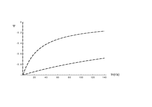
FIG. 2.: The solid curves are the exact relative correction $\Psi(r/a)$, given by Eq. (62), and the dashed curves are approximate relative correction, given by Eq. (63), for the flower-pot model with $\xi=1/6$ and $\kappa=10/9$ (upper curves) and $\kappa=100/99$ (lower curves).

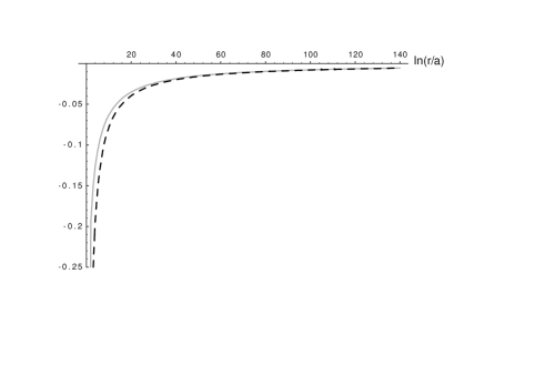
FIG. 3.: The solid curve is the (scaled) exact self-energy $W_{\rm super}(r)\times(4\pi\epsilon_{0}/Q^{2})r$ and the dashed curve is the (scaled) approximate self-energy $W_{\rm super}(r)\times(4\pi\epsilon_{0}/Q^{2})r$ for perfect conductor boundary conditions on a superconducting string with $\kappa=100/99$. The gravitational contribution to the (scaled) self-energy is given by the straight line $W_{\rm reg}\times(4\pi\epsilon_{0}/Q^{2})r={\cal K}(100/99)/2\approx 0{\cdot}0020$.

REFERENCES

- [1] E. Witten, Nucl.Phys. B249, 557 (1985).
- [2] A.G. Smith in Symposium on the Formation and Evolution of Cosmic Strings, edited by G.W. Gibbons, S.W. Hawking, and T. Vachaspati (Cambridge University Press, Cambridge, 1989). Note that Gaussian units are used in this reference whereas we are using SI units.
- [3] B. Linet, Phys.Rev.D 33, 1833 (1986).
- [4] B. Allen and A.C. Ottewill, Phys.Rev.D 42, 2669 (1990).
- [5] B.S. Kay and U.M. Studer, Commun.Math.Phys. 139, 103 (1991).
- [6] In terms of the notion of self-adjoint extensions, the Laplace-Beltrami operator for a constant-time 3-dimensional spatial section of the idealized string metric, when defined on the domain of smooth functions compactly supported away from line in the space of square-integrable functions on the spatial section, has a one-parameter family of -translationally invariant self-adjoint extensions (corresponding to unrestricted self-adjoint extensions for the 2-dimensional Laplace-Beltrami operator on sections of constant and ) which are labelled by the parameter taking its values in , with the case corresponding to regular boundary conditions, and non-zero to the behaviour (3).
- [7] R.M. Wald, Commun.Math.Phy. 70, 221 (1979).
- [8] See, for example, the review article by J.S. Dowker in Symposium on the Formation and Evolution of Cosmic Strings, edited by G.W. Gibbons, S.W. Hawking, and T. Vachaspati (Cambridge University Press, Cambridge, 1989).
- [9] Note that only the leading asymptotic form for for the ‘flower-pot’ was given in Ref.[4]. The next term which is important here was given in B. Allen, J.G. McLaughlin and A.C. Ottewill, Phys.Rev.D 45, 4486 (1992).
- [10] B.S. Kay, Phys.Rev.D 20, 3052 (1979).
- [11] M.R.Brown and A.C. Ottewill, Phys.Rev.D 34, 1776 (1986).
- [12] B.S. Kay and C.J. Fewster, When Can A Small Object Have a Big Effect at Large Scales? – in preparation.
- [13] S. Albeverio, F. Gesztesy, R. Hoegh-Krohn and H. Holden, Solvable Models in Quantum Mechanics, (Springer-Verlag, New York, 1988).
- [14] I.S. Gradsteyn and I.M. Ryzhik, Tables of Integrals, Series and Products, (Academic Press, New York, 1980)