Uncertainties of predictions in models of eternal inflation

Abstract

In a previous paper [1], a method of comparing the volumes of thermalized regions in eternally inflating universe was introduced. In this paper, we investigate the dependence of the results obtained through that method on the choice of the time variable and factor ordering in the diffusion equation that describes the evolution of eternally inflating universes. It is shown, both analytically and numerically, that the variation of the results due to factor ordering ambiguity inherent in the model is of the same order as their variation due to the choice of the time variable. Therefore, the results are, within their accuracy, free of the spurious dependence on the time parametrization.

98.80.Hw

I Introduction

The parameters we call “constants of Nature” can take different values in different parts of the universe and in different disconnected universes in the ensemble described by the cosmological wave function [2, 3]. The probability distribution for the constants can be determined with the aid of the “principle of mediocrity” [4, 5], which asserts that we are “typical” among the civilizations inhabiting this ensemble. The resulting probabilities are then proportional to the physical volumes occupied by thermalized regions with given values of the constants [6], and the preferred values tend to be the ones that give the largest amount of inflation.

This prescription encounters a difficulty when applied to models where inflation is “eternal”. In such models, the universe consists of a number of isolated thermalized regions embedded in a still-inflating background. New thermalized regions are constantly being formed, but the inflating domains that separate them expand so fast that the universe never thermalizes completely [7, 8]. In an eternally inflating universe, the thermalized volumes ${\cal V}_{*}^{(j)}$ diverge as $t\rightarrow\infty$. (Here, the index $j$ labels different types of thermalized regions which have different values of the constants of Nature.) If one simply introduces a time cutoff by including only parts of the volumes that thermalized prior to some moment of time $t_{c}$, then one finds that the ratio

$\displaystyle r=\lim_{t_{c}\rightarrow\infty}\frac{{\cal V}_{*}^{\left(1\right)}}{{\cal V}_{*}^{\left(2\right)}}$

is extremely sensitive to the choice of the time coordinate $t$. For example, cutoffs at a fixed proper time and at a fixed scale factor give drastically different results [9]. An alternative procedure [1] is to introduce a cutoff at the time $t_{c}^{(j)}$ when all but a small fraction $\varepsilon$ of the co-moving volume destined to thermalize into regions of type $j$ has thermalized. The value of $\varepsilon$ is taken to be the same for all types of thermalized regions, and for all universes in the ensemble, but the corresponding cutoff times $t_{c}^{(j)}$ are generally different. The limit $\varepsilon\rightarrow 0$ is taken after calculating the probability distribution for the constants. It was shown in [1] that the resulting probabilities are rather insensitive to the choice of time parametrization.

Although this can certainly be regarded as progress, the situation is still not completely satisfactory. What do we make of the residual, “mild” dependence of the probabilities on the choice of the time coordinate $t$? This dependence is particularly worrisome when one tries to compare probabilities for different universes in the quantum-cosmological ensemble. Using the $\varepsilon$-procedure, one finds [1] that the probability distribution has an infinitely sharp peak at the highest value of the ratio $\tilde{\gamma}/\gamma$, where $-\tilde{\gamma}$ and $\gamma$ are the smallest eigenvalues of the diffusion equation for the probability distribution of the inflaton field $\varphi$, with normalization to the physical and coordinate volume, respectively. This sharp prediction does not mix well even with a “mild” ambiguity in the value of $\tilde{\gamma}/\gamma$.

An additional source of ambiguity in predictions of eternal inflation is in the form of the diffusion equation itself. The equation was introduced in Refs. [7, 9, 12, 13, 14, 15] to describe the effect of quantum fluctuations on the evolution of the inflaton field. It gives accurate results for sufficiently flat inflaton potentials $V\left(\varphi\right)$, provided that the magnitude of $V\left(\varphi\right)$ is well below the Planck energy density, $V\left(\varphi\right)\ll 1$. [Here and below we use Planck units in which $\hbar=c=G=1$.] By its nature, however, the equation is an approximation to quantum field theory in a curved spacetime, or, if gravity is to be adequately included, to the Wheeler-DeWitt equation for the cosmological wave function. This approximate nature of the diffusion equation manifests itself, in particular, in the ambiguity in the ordering of factors $\partial/\partial\varphi$ and $D\left(\varphi\right)$, where $D\left(\varphi\right)$ is the field-dependent diffusion coefficient.

In the present paper we shall analyze the uncertainties in predictions of the principle of mediocrity resulting both from the choice of the time parameter and of the factor-ordering in the diffusion equation. It will be shown that the uncertainties of the probabilities due to these two ambiguities are of the same order of magnitude. Since the factor-ordering ambiguity is inherent in the diffusion approximation, the corresponding uncertainty can be regarded as the bound on the accuracy allowed by the model. Our result is then that, within this accuracy, the probabilities are independent of time parametrization. This is a hopeful sign, since it suggests that a complete independence of time parametrization can be achieved in a more fundamental approach.

The paper is organized as follows. In the next section, we introduce the necessary formalism. Sections III and IV present our analytic and numerical results. Conclusions and a discussion of some open issues follow in section V.

II The diffusion equation

We shall consider “new” inflation with a potential $V\left(\varphi\right)$ of the form illustrated in Fig. 1. The potential has two minima and the values $\varphi_{*}^{\left(1\right)}$ and $\varphi_{*}^{\left(2\right)}$ near the minima correspond to the end of inflation. We will be interested in the relative probability ${\cal P}^{\left(2\right)}/{\cal P}^{\left(1\right)}$ for the two minima. In this section, we shall first introduce the parameters $\alpha$ and $\beta$, representing the freedom of time parametrization and factor ordering. We shall then bring the diffusion equation to a convenient self-adjoint form, and finally derive a general expression for ${\cal P}^{\left(2\right)}/{\cal P}^{\left(1\right)}$.

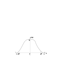
FIG. 1.: Inflaton potential for a new inflationary scenario.

A Parametrization of choices of time and factor ordering

The evolution of the inflaton field $\varphi$ during inflation can be described by a probability distribution $P\left(\varphi,t\right)d\varphi$ which is interpreted, up to a normalization, as the (either co-moving or physical) volume of regions with a particular value of $\varphi$ in the interval $d\varphi$. We shall use the notation $P\left(\varphi,t\right)$ for the co-moving and $\tilde{P}\left(\varphi,t\right)$ for the physical volume probability. The latter satisfies the diffusion equation which can be written as

$$\partial_{t}\tilde{P}=\partial_{\varphi}\left[D\left(\varphi\right)^{1/2+\beta}\partial_{\varphi}\left(D\left(\varphi\right)^{1/2-\beta}\tilde{P}\right)-v\left(\varphi\right)\tilde{P}\right]+3H\left(\varphi\right)^{\alpha}\tilde{P}$$ (1)

where

$\displaystyle H\left(\varphi\right)=\sqrt{\frac{8\pi}{3}V\left(\varphi\right)}$

is the Hubble constant, $V\left(\varphi\right)$ is the inflaton potential, $D\left(\varphi\right)$ is the diffusion coefficient,

$$D\left(\varphi\right)=\frac{1}{8\pi^{2}}H\left(\varphi\right)^{\alpha+2},$$ (2)

and

$$v\left(\varphi\right)=-\frac{1}{4\pi}H\left(\varphi\right)^{\alpha-1}\partial_{\varphi}H\left(\varphi\right)$$ (3)

is the average “drift velocity” corresponding to the slow roll. Eq. (1) is accurate provided that the condition of slow roll,

$$\left|H^{\prime}\left(\varphi\right)\right|\ll 2\pi H\left(\varphi\right),$$ (4)

is satisfied.

The initial distribution $\tilde{P}\left(\varphi,t=0\right)$ can be derived from the cosmological wave function of the nucleated universe [16]. For the “tunneling” wave function,

$$\tilde{P}\left(\varphi,t=0\right)\propto\exp\left(-\frac{3}{8V\left(\varphi\right)}\right).$$ (5)

Essentially the same results are obtained by taking any bell-shaped initial distribution peaked around the maximum of the inflaton potential $V\left(\varphi\right)$.

The solution is subject to the following boundary conditions at thermalization points $\varphi=\varphi_{*}^{\left(1,2\right)}$:

$$D\left(\varphi\right)^{1/2+\beta}\partial_{\varphi}\left(D\left(\varphi\right)^{1/2-\beta}P\right)=0.$$ (6)

The boundary condition (6) means that diffusion is constrained to vanish at points $\varphi_{*}^{\left(1,2\right)}$ which are found from the “thermalization condition”,

$$\left|H^{\prime}\left(\varphi_{*}^{\left(1,2\right)}\right)\right|\simeq 2\pi H\left(\varphi_{*}^{\left(1,2\right)}\right).$$ (7)

This equality signifies the breakdown of the slow roll condition (4). Since (7) is an order-of-magnitude relation, the exact values of $\varphi_{*}^{\left(1,2\right)}$ depend on the choice of the constant of order $1$ in (7). Although this introduces an ambiguity in our model, we note that diffusion, which represents quantum fluctuations, is already negligibly small in the regions dominated by the slow roll, and the ambiguity in the choice of points $\varphi_{*}^{\left(1,2\right)}$ at which diffusion is constrained to exactly vanish does not significantly influence the solution of the diffusion equation [17]. The “no-diffusion” boundary condition (6) was introduced in [9].

In equation (1), different choices of time variable and factor ordering are represented by choices of the parameters $\alpha$ and $\beta$. The parameter $\alpha$ is equal to the physical dimension of the time variable $t$, which is related to the proper time $\tau$ by

$$dt=H\left(\varphi\right)^{1-\alpha}d\tau$$ (8)

(so that $\alpha=1$ corresponds to the proper time parametrization, $t=\tau$, and $\alpha=0$ corresponds to using the scale factor as a time variable). The choice of the factor ordering is parametrized by $\beta$ which is defined so that $\beta=0$ gives the so called Stratonovich factor ordering [9, 12]. A similar parametrization of factor ordering in the diffusion equation (1) was used by Salopek and Bond [25].

The equation for the coordinate-volume distribution $P\left(\varphi,t\right)$ is identical to (1), except for the absence of the expansion term:

$$\partial_{t}P=\partial_{\varphi}\left[D\left(\varphi\right)^{1/2+\beta}\partial_{\varphi}\left(D\left(\varphi\right)^{1/2-\beta}P\right)-v\left(\varphi\right)P\right]$$ (9)

More generally, one could consider a time variable related to the proper time $\tau$ by

$$dt=T\left(\varphi\right)d\tau,$$ (10)

with $T\left(\varphi\right)$ an arbitrary function; the choice (8) corresponds to $T\left(\varphi\right)=H\left(\varphi\right)^{1-\alpha}$. With a general time function, the diffusion coefficient would change to

$$D\left(\varphi\right)=\frac{H\left(\varphi\right)^{3}}{8\pi^{2}T\left(\varphi\right)}$$ (11)

and the drift velocity would become

$$v\left(\varphi\right)=-\frac{H^{\prime}}{4\pi T\left(\varphi\right)}.$$ (12)

Also, the factor ordering in Eqs. (1),(9) could be generalized to insertion of an arbitrary function $h\left(\varphi\right)$ which would change the diffusion term in those equations to

$$D\left(\varphi\right)^{1/2+\beta}\partial_{\varphi}\left(D\left(\varphi\right)^{1/2-\beta}P\right)\rightarrow D\left(\varphi\right)^{1/2}h\left(\varphi\right)\partial_{\varphi}\left(D\left(\varphi\right)^{1/2}\frac{1}{h\left(\varphi\right)}P\right).$$ (13)

The factor ordering of Eqs. (1),(9) corresponds to the choice $h\left(\varphi\right)=D\left(\varphi\right)^{\beta}$.

We will not consider these possibilities here, since the physical reasons for the “correct” choice of functions $T\left(\varphi\right)$ and $h\left(\varphi\right)$ are not clear. In the following discussion, we shall use exclusively the parameters $\alpha$ and $\beta$ to explore the ambiguities related to these choices.

B Self-adjoint form of the diffusion equation

The late-time behavior of the distribution functions described by Eqs. (1),(9) is determined by the eigenfunctions

$$P\left(\varphi,t\right)=e^{-\gamma t}\psi^{\left(1\right)}\left(\varphi\right),\quad\tilde{P}\left(\varphi,t\right)=e^{\tilde{\gamma}t}\tilde{\psi}^{\left(1\right)}\left(\varphi\right),$$ (14)

having highest eigenvalues $\tilde{\gamma}$ and $-\gamma$. The equations for $\tilde{\psi}\left(\varphi\right)$ and $\psi\left(\varphi\right)$ are stationary forms of (1),(9),

$$\partial_{\varphi}\left[D\left(\varphi\right)^{1/2+\beta}\partial_{\varphi}\left(D\left(\varphi\right)^{1/2-\beta}\tilde{P}\right)-v\left(\varphi\right)\tilde{P}\right]+3H\left(\varphi\right)^{\alpha}\tilde{P} = \tilde{\gamma}\tilde{P},$$ (15)

$$\partial_{\varphi}\left[D\left(\varphi\right)^{1/2+\beta}\partial_{\varphi}\left(D\left(\varphi\right)^{1/2-\beta}P\right)-v\left(\varphi\right)P\right] = -\gamma P.$$ (16)

The sign convention in the definition of $\gamma$ and $\tilde{\gamma}$ reflects the fact that the highest value of $\tilde{\gamma}$ and the smallest value of $\gamma$ are both positive. (If the highest value of $\tilde{\gamma}$ is negative, then there is no eternal inflation. See also section III A below.)

Equations (15),(16) can be transformed to a manifestly self-adjoint form [18]. One introduces a new independent variable $z$,

$$z=\int\left[2D\left(\varphi\right)\right]^{-1/2}d\varphi,\quad P\left(\varphi\right)=\left[2D\left(\varphi\right)\right]^{-1/2}f\left(z\right),$$ (17)

and a further substitution

$$f\left(z,t\right)=g\left(z,t\right)D\left(z\right)^{\beta/2}\exp\left(\frac{\pi}{2H\left(z\right)^{2}}\right)\equiv g\left(z,t\right)\exp\left(\int b\left(z\right)dz\right),$$ (18)

where we have defined

$$b\left(z\right)=-\pi\frac{H_{z}^{\prime}}{H^{3}}+\frac{\beta}{2}\frac{D_{z}^{\prime}}{D}.$$ (19)

Equation (9) then leads to the following equation for $g\left(z,t\right)$:

$$\partial_{t}g=\frac{1}{2}\partial_{zz}g+(-\frac{1}{2}b_{z}^{\prime}-\frac{1}{2}b^{2})g.$$ (20)

This form of the equation was derived in [14] for the case of $\alpha=\beta=0$.

Under the same transformations, equation (1) for the physical-volume distribution becomes

$$\partial_{t}\tilde{g}=\frac{1}{2}\partial_{zz}\tilde{g}+\left(-\frac{1}{2}b_{z}^{\prime}-\frac{1}{2}b^{2}+3H^{\alpha}\right)\tilde{g},$$ (21)

The transformed versions of Eqs. (15),(16) can be written as:

$$-\frac{1}{2}\tilde{g}^{\prime\prime}+\left(\frac{1}{2}b_{z}^{\prime}+\frac{1}{2}b^{2}-3H^{\alpha}\right)\tilde{g} = -\tilde{\gamma}\tilde{g},$$ (22)

$$-\frac{1}{2}g^{\prime\prime}+\left(\frac{1}{2}b_{z}^{\prime}+\frac{1}{2}b^{2}\right)g = \gamma g,$$ (23)

where primes denote differentiation with respect to $z$. The boundary conditions (6) become

$$\partial_{z}\left[D^{-\beta/2}\exp\left(\frac{\pi}{2H^{2}}\right)g\left(z\right)\right]=0,$$ (24)

and they are to be imposed at points $z_{*}^{\left(1,2\right)}$ corresponding to the thermalization points $\varphi_{*}^{\left(1,2\right)}$ of (7).

Equations (22),(23) have the form of a stationary Schrödinger equation for a one-dimensional motion in a potential $U\left(z\right)$,

$$-\frac{1}{2}g^{\prime\prime}+U\left(z\right)g=Eg,$$ (25)

with

$$\tilde{U}\left(z\right)=\frac{1}{2}b^{\prime}+\frac{1}{2}b^{2}-3H^{\alpha}$$ (26)

for the physical-volume distribution and

$$U\left(z\right)=\frac{1}{2}b^{\prime}+\frac{1}{2}b^{2}$$ (27)

for the coordinate-volume distribution. With boundary conditions (24), the operator $\left(-1/2\right)\partial_{zz}$ appearing in the left hand side of (25) is non-negative if

$$\int\limits_{z_{*}^{\left(1\right)}}^{z_{*}^{\left(2\right)}}g\left(z\right)\left(-\frac{1}{2}\partial_{zz}g\right)dz=\left[-g\left(z\right)^{2}\frac{H_{z}^{\prime}}{4H^{3}}\left(2\pi+H^{2}\beta\left(\alpha+2\right)\right)\right]_{z_{*}^{\left(1\right)}}^{z_{*}^{\left(2\right)}}+\frac{1}{2}\int\limits_{z_{*}^{\left(1\right)}}^{z_{*}^{\left(2\right)}}\left[g^{\prime}\left(z\right)\right]^{2}dz\geq 0$$ (28)

for any function $g\left(z\right)$. This holds for a potential of Fig. 1 since $V^{\prime}\left(\varphi_{*}^{\left(2\right)}\right)<0$ and $V^{\prime}\left(\varphi_{*}^{\left(1\right)}\right)>0$ and so $H_{z}^{\prime}\left(z_{*}^{\left(2\right)}\right)<0$ and $H_{z}^{\prime}\left(z_{*}^{\left(1\right)}\right)>0$. Therefore, the eigenvalues $E$ of (25) are bounded from below by the minimum values of the potentials (26) and (27), and we denote $-\tilde{\gamma}$ and $\gamma$ the lowest eigenvalues of the respective operators, as defined by (22),(23), with eigenfunctions $\tilde{\psi}^{\left(1\right)}$ and $\psi^{\left(1\right)}$. Exact solutions for $\tilde{\psi}^{\left(1\right)}$ and $\psi^{\left(1\right)}$ can be found for special cases of the inflaton potential $V\left(\varphi\right)$ (and special values of the parameters $\alpha$, $\beta$) for which the Schrödinger equation is exactly solvable (see Appendix A).

Since the boundary conditions (24) are homogeneous, the operator $\left(-1/2\right)\partial_{zz}+U\left(z\right)$ in (25) is self-adjoint, and its eigenfunctions are orthogonal with respect to the usual scalar product,

$$\left\langle g_{1}\left(z\right),g_{2}\left(z\right)\right\rangle\equiv\int g_{1}\left(z\right)g_{2}\left(z\right)dz.$$ (29)

In the original variables, this scalar product becomes

$$\left\langle P_{1}\left(\varphi\right),P_{2}\left(\varphi\right)\right\rangle=\int P_{1}\left(\varphi\right)P_{2}\left(\varphi\right)\frac{\sqrt{2D\left(\varphi\right)}}{D\left(\varphi\right)^{\beta}}\exp\left(-\frac{\pi}{H\left(\varphi\right)^{2}}\right)d\varphi.$$ (30)

Using the scalar product (30), the solution of the time-dependent equation (9) with a given initial distribution $P\left(\varphi,t=0\right)\equiv P_{0}\left(\varphi\right)$ can be expressed through the orthonormal eigenfunctions $\psi^{\left(1\right)}$, $\psi^{\left(2\right)}$, $\psi^{\left(3\right)}$, … with eigenvalues $\gamma_{\left(1\right)}\equiv-\gamma$, $\gamma_{\left(2\right)}$, $\gamma_{\left(3\right)}$, …, as

$$P\left(\varphi,t\right)=\sum_{n=1}^{\infty}C_{n}\exp\left(\gamma_{\left(n\right)}t\right)\psi^{\left(n\right)}\left(\varphi\right),$$ (31)

with the coefficients $C_{n}$ given by

$$C_{n}=\left\langle P_{0}\left(\varphi\right),\psi^{(n)}\left(\varphi\right)\right\rangle,$$ (32)

and similarly for $\tilde{P}\left(\varphi,t\right)$. Note that co-moving and physical volumes coincide at $t=0$, and thus $\tilde{P}\left(\varphi,0\right)=P\left(\varphi,0\right)$.

C The ratio of physical volumes, $r$

The quantities of interest to us are the volumes ${\cal V}_{*}^{\ (j)}$ of the thermalization hypersurfaces $\varphi=\varphi_{*}^{(j)}$. To express these volumes in terms of the eigenfunctions (14), we first rewrite the diffusion equations (1),(9) as continuity equations:

$$\partial_{t}\tilde{P} = -\partial_{\varphi}\tilde{J}+3H^{\alpha}\tilde{P},$$ (33)

$$\partial_{t}P = -\partial_{\varphi}J.$$ (34)

Here, the fluxes $\tilde{J}$, $J$ are related to the distribution functions $\tilde{P}$, $P$ by

$$J=-D\left(\varphi\right)^{1/2+\beta}\partial_{\varphi}\left(D\left(\varphi\right)^{1/2-\beta}P\right)+v\left(\varphi\right)P.$$ (35)

From the continuity equation (34) it follows that the loss of co-moving volume in inflating regions is compensated by the corresponding growth in the volume of the thermalized regions. The rate of this growth is given by the flux through the thermalization points:

$$\frac{\partial}{\partial t}\int\limits_{\varphi_{*}^{\left(1\right)}}^{\varphi_{*}^{\left(2\right)}}P\left(\varphi,t\right)d\varphi=\left.\left(-J\right)\right|_{\varphi_{*}^{\left(1\right)}}^{\varphi_{*}^{\left(2\right)}}.$$ (36)

Therefore, the co-moving volume ${\cal V}_{(c)*}^{\left(1,2\right)}$ thermalized in a specific minimum of the inflaton potential throughout a given time range is

$${\cal V}_{(c)*}^{\left(1,2\right)}=\left|\int\limits_{t_{1}}^{t_{2}}J\left(\varphi_{*}^{\left(1,2\right)},t\right)dt\right|$$ (37)

(the absolute value is needed to cancel the negative sign of the flux through the leftmost thermalization point). We use a similar formula for the thermalized physical volume:

$${\cal V}_{*}^{\left(1,2\right)}=\left|\int\limits_{t_{1}}^{t_{2}}\tilde{J}\left(\varphi_{*}^{\left(1,2\right)},t\right)dt\right|$$ (38)

According to the method proposed in [1], the infinite thermalization volumes

$${\cal V}_{*}^{\left(1,2\right)}=\left|\int\limits_{0}^{t_{\varepsilon}^{\left(1,2\right)}}\tilde{J}\left(\varphi_{*}^{\left(1,2\right)},t\right)dt\right|=\left|\int\limits_{0}^{t_{\varepsilon}^{\left(1,2\right)}}v\left(\varphi_{*}^{\left(1,2\right)}\right)\tilde{P}\left(\varphi_{*}^{\left(1,2\right)},t\right)dt\right|$$ (39)

are to be cut off at times $t_{\varepsilon}^{\left(1,2\right)}$ which are determined from the condition that only a fraction $\varepsilon$ of the corresponding co-moving volume is left unthermalized at those times,

$$\left|\int\limits_{t_{\varepsilon}^{\left(1,2\right)}}^{\infty}J\left(\varphi_{*}^{\left(1,2\right)},t\right)dt\right|=\varepsilon\left|\int\limits_{0}^{\infty}J\left(\varphi_{*}^{\left(1,2\right)},t\right)dt\right|\equiv\varepsilon p_{1,2}.$$ (40)

Here, $p_{1}$ and $p_{2}$ are fractions of the total co-moving volume (averaged over an ensemble of universes) that will eventually thermalize in the first and the second minima of the inflaton potential, respectively.

The integrals in (39),(40) are dominated by the ground state eigenfunctions (14) of (15),(16) which we have denoted by $\tilde{\psi}^{\left(1\right)}\left(\varphi\right)$ and $\psi^{\left(1\right)}\left(\varphi\right)$. Using (31) for $P\left(\varphi_{*}^{\left(1,2\right)},t\right)$, we obtain

$$\int\limits_{t_{\varepsilon}^{\left(1,2\right)}}^{\infty}J\left(\varphi_{*}^{\left(1,2\right)},t\right)dt=\int\limits_{t_{\varepsilon}^{\left(1,2\right)}}^{\infty}v\left(\varphi_{*}^{\left(1,2\right)}\right)P\left(\varphi_{*}^{\left(1,2\right)},t\right)dt\approx\frac{C_{1}\exp\left(-\gamma t_{\varepsilon}^{\left(1,2\right)}\right)}{\gamma}v\left(\varphi_{*}^{\left(1,2\right)}\right)\psi^{\left(1\right)}\left(\varphi_{*}^{\left(1,2\right)}\right).$$ (41)

After solving (40),(41) for $t_{\varepsilon}^{\left(1,2\right)}$, one can calculate from (39) the ratio of the physical volumes that thermalize in the two minima of the inflaton potential:

$$r\equiv\frac{{\cal V}_{*}^{\left(2\right)}}{{\cal V}_{*}^{\left(1\right)}}=\frac{\left|v_{2}\right|\tilde{\psi}_{2}}{\left|v_{1}\right|\tilde{\psi}_{1}}\left(\frac{\left|v_{2}\right|\psi_{2}}{\left|v_{1}\right|\psi_{1}}\frac{p_{1}}{p_{2}}\right)^{\tilde{\gamma}/\gamma},$$ (42)

where

$$\psi_{1,2}\equiv\psi^{\left(1\right)}\left(\varphi_{*}^{\left(1,2\right)}\right),\quad\tilde{\psi}_{1,2}\equiv\tilde{\psi}^{\left(1\right)}\left(\varphi_{*}^{\left(1,2\right)}\right)$$ (43)

are the values of the ground state eigenfunctions taken at thermalization points $\varphi_{*}^{\left(1,2\right)}$, and

$$v_{1,2}\equiv\left.-\frac{H^{\alpha-1}H^{\prime}}{4\pi}\right|_{\varphi_{*}^{\left(1,2\right)}}$$ (44)

are “drift velocities” at those points.

D Ambiguities in $r$

The form of the diffusion equations (1),(9) depends on the parameters $\alpha$ and $\beta$, and therefore the quantities $\gamma$, $\tilde{\gamma}$, $\psi_{j}$, $\tilde{\psi}_{j}$, $p_{j}$ appearing in Eq. (42) for the volume ratio $r$ all depend on $\alpha$ and $\beta$. This dependence, which reflects the sensitivity of $r$ to the choice of the time parametrization and of the factor ordering, is the main focus of the present paper and will be analyzed in detail in the following two sections.

Another source of uncertainty is the choice of the initial distribution $P\left(\varphi,0\right)\equiv P_{0}\left(\varphi\right)$ for the calculation of $p_{j}$. If we choose a Gaussian distribution peaked at the maximum of the potential $V\left(\varphi\right)$ and having a width $w$ much smaller than the characteristic width of the maximum, then the values of $p_{j}$ should not be very sensitive to $w$. But a weak dependence of $p_{j}$ on $w$ certainly exists and should be addressed as a matter of principle. Some numerical results on this $w$-dependence will be presented in Section IV.

The problem of initial distribution can be resolved by invoking quantum cosmology and using a distribution, like Eq. (5), obtained from the cosmological wave function. However, it has been argued [19] that probability is an approximate concept in quantum cosmology and can be defined only within the semiclassical approximation. The accuracy of this approximation for a nucleating universe is characterized by $S^{-1}=H_{0}^{2}/\pi$, where $S$ is the tunneling action and $H_{0}$ is the value of $H$ at the maximum of $V\left(\varphi\right)$. Hence, it may be impossible to reduce the uncertainty in $P_{0}\left(\varphi\right)$ below $O\left(H_{0}^{2}\right)$.

Yet another uncertainty in (42), this time rather benign, is related to the already mentioned choice of the constant of order $1$ in (7) which affects the exact values of thermalization points $\varphi_{*}^{\left(1,2\right)}$. A different choice will change the behavior of the solution $\tilde{\psi}^{\left(1\right)}\left(\varphi\right)$ near $\varphi=\varphi_{*}^{\left(1,2\right)}$ (the derivative $\tilde{\psi}^{\prime}\left(\varphi\right)$ changes sign at $\varphi_{*}^{\left(1,2\right)}$ [9]). However, since the diffusion term in (35) is negligible at those points, one can employ the asymptotic formulae [1]

$$\tilde{\psi}^{\left(1\right)}\left(\varphi\right)\approx\tilde{c}\frac{H\left(\varphi\right)}{H^{\prime}\left(\varphi\right)}\exp\left[-12\pi\int_{\varphi_{0}}^{\varphi}\frac{H\left(\varphi\right)d\varphi}{H^{\prime}\left(\varphi\right)}+4\pi\tilde{\gamma}\int_{\varphi_{0}}^{\varphi}\frac{H^{1-\alpha}\left(\varphi\right)d\varphi}{H^{\prime}\left(\varphi\right)}\right],$$ (45)

$$\psi^{\left(1\right)}\left(\varphi\right)\approx c\frac{H\left(\varphi\right)}{H^{\prime}\left(\varphi\right)}\exp\left[-4\pi\gamma\int_{\varphi_{0}}^{\varphi}\frac{H^{1-\alpha}\left(\varphi\right)d\varphi}{H^{\prime}\left(\varphi\right)}\right],$$ (46)

which are accurate in the deterministic slow roll region up to the neglected diffusion term. Here, $\varphi_{0}$ is some point in the region where diffusion is negligible,

$$H^{2}\left(\varphi_{0}\right)\ll\frac{\partial H}{\partial\varphi}\left(\varphi_{0}\right).$$ (47)

With the help of (45)-(46), one can show that a change in thermalization points $\varphi_{*}^{\left(1,2\right)}\rightarrow\bar{\varphi}_{*}^{\left(1,2\right)}$ changes the ratio (42) by the ratio of the additional volume expansion factors gained before thermalization,

$$r\rightarrow r\frac{\exp\left(-12\pi\int_{\varphi_{*}^{\left(2\right)}}^{\bar{\varphi}_{*}^{\left(2\right)}}\frac{H\left(\varphi\right)d\varphi}{H^{\prime}\left(\varphi\right)}\right)}{\exp\left(-12\pi\int_{\varphi_{*}^{\left(1\right)}}^{\bar{\varphi}_{*}^{\left(1\right)}}\frac{H\left(\varphi\right)d\varphi}{H^{\prime}\left(\varphi\right)}\right)}.$$ (48)

To obtain unambiguous relative probabilities, one could compare the volumes of constant-temperature hypersurfaces with the same value of $T$ in different types of regions. Then one would have to multiply ${\cal V}_{*}^{(j)}$ by the additional expansion factors up to the chosen temperature, and the dependence on the precise values of $\varphi_{*}^{\left(1,2\right)}$ would disappear.

III Analytic estimates

A Estimate of eigenvalues

Perhaps the most important parameters entering (42), in terms of their effect on the magnitude of $r$, are the ground state eigenvalues of Eqs. (15),(16). These eigenvalues $\tilde{\gamma}$, $\gamma$ can be estimated if the inflaton potential is sufficiently flat and smooth near its maximum. The estimate is based on expansion of the effective potential $U\left(z\right)$ of the Schrödinger equation (25) around its minimum up to terms quadratic in $z$.

We shall assume for simplicity that the inflaton potential is symmetric around its maximum at $\varphi=0$ up to terms of quartic order in $\varphi$. Then the expansion of $H\left(\varphi\right)$ around $\varphi=0$ has the form

$$H\left(\varphi\right)=H_{0}+\frac{H_{2}}{2}\varphi^{2}+\frac{H_{4}}{24}\varphi^{4}+O\left(\varphi^{5}\right)$$ (49)

with $H_{0}>0$ and $H_{2}<0$. The diffusion coefficient (2) is also expanded as

$$D\left(\varphi\right) = D_{0}+\frac{D_{2}}{2}\varphi^{2}+O\left(\varphi^{4}\right),$$ (51)

$$D_{0} = \frac{H_{0}^{\alpha+2}}{8\pi^{2}},\quad D_{2}=\frac{\left(\alpha+2\right)H_{0}^{\alpha+1}H_{2}}{8\pi^{2}}.$$ (52)

We then use (17) to find the derivatives with respect to $z$ at the point $z=0$ corresponding to $\varphi=0$,

$$\left.\frac{\partial H}{\partial z}\right|_{z=0} = 0,\quad\left.\frac{\partial^{2}H}{\partial z^{2}}\right|_{z=0}=2D_{0}H_{2},$$ (54)

$$\left.\frac{\partial^{3}H}{\partial z^{3}}\right|_{z=0} = 0,\quad\left.\frac{\partial^{4}H}{\partial z^{4}}\right|_{z=0}=8D_{0}D_{2}H_{2}+4D_{0}^{2}H_{4},$$ (55)

and substitute them into (19),(26) and (27) to obtain the expansion of the effective Schrödinger potential,

$$U\left(z\right)=U_{0}+\frac{\omega^{2}}{2}z^{2}+O\left(z^{3}\right).$$ (56)

The coefficients $U_{0}$ and $\omega$ for the potential (27) are given by

$$U_{0} = \left|H_{2}\right|\frac{H_{0}^{\alpha-1}}{8\pi}\left(1-\beta H_{0}^{2}\frac{\alpha+2}{2\pi}\right),$$ (58)

$$\omega^{2} = H_{2}^{2}\frac{H_{0}^{2\alpha-2}}{16\pi^{2}}\left(1-\frac{H_{0}^{2}}{2\pi}\left[-5+2\alpha+2\beta\left(2+\alpha\right)+\frac{H_{4}H_{0}}{H_{2}^{2}}\right]+O\left(H_{0}^{4}\right)\right)$$ (59)

and for the potential (26)

$$\tilde{U}_{0} = U_{0}-3H_{0}^{\alpha}=-3\,H_{0}^{\alpha}+\left|H_{2}\right|\frac{H_{0}^{\alpha-1}}{8\pi}\left(1-\beta H_{0}^{2}\frac{\alpha+2}{2\pi}\right),$$ (61)

$$\tilde{\omega}^{2} = H_{2}^{2}\frac{H_{0}^{2\alpha-2}}{16\pi^{2}}\left(1+12\alpha\frac{H_{0}^{3}}{\left|H_{2}\right|}-\frac{H_{0}^{2}}{2\pi}\left[-5+2\alpha+2\beta\left(2+\alpha\right)+\frac{H_{4}H_{0}}{H_{2}^{2}}\right]+O\left(H_{0}^{4}\right)\right).$$ (62)

This analysis can be generalized to non-symmetric potentials with $H^{\prime\prime\prime}\left(0\right)\neq 0$; in that case, the minimum of $U\left(z\right)$ will be shifted from $z=0$.

Assuming that the quadratic expansion (56) of the potential $U\left(z\right)$ is accurate enough up to the classical turning points, we can approximate the eigenvalues of (25) by the corresponding eigenvalues of the harmonic oscillator,

$$E_{n}=U_{0}+\frac{\omega}{2}+n\omega,$$ (63)

and the ground state eigenvalues by

$$-\tilde{\gamma} = \tilde{U}_{0}+\frac{\tilde{\omega}}{2},$$ (64)

$$\gamma = U_{0}+\frac{\omega}{2}.$$ (65)

Although our boundary conditions are not the same as those for the harmonic oscillator eigenvalues (63), they are imposed at points $\varphi_{*}^{(1,2)}$ deeply within the classically forbidden region of the Schrödinger equation and it seems reasonable to assume that a different choice of these boundary conditions does not significantly alter the eigenvalues. The validity of the estimates (64)-(65) was confirmed numerically (see Section IV).

We assume that the potential $V\left(\varphi\right)$ is flat near its maximum and that the maximum value $V\left(0\right)$ is small in Planck units:

$$\frac{\left|H_{2}\right|}{H_{0}}=\left.\frac{\left|V^{\prime\prime}\right|}{2V}\right|_{\varphi=0}\ll 1,\quad H_{0}^{2}=\frac{8\pi V\left(0\right)}{3}\ll 1.$$ (66)

We also assume that

$$\frac{H_{4}H_{0}}{H_{2}^{2}}=-3+2\left.\frac{V^{\left(\text{IV}\right)}V}{\left(V^{\prime\prime}\right)^{2}}\right|_{\varphi=0}\lesssim 1,$$ (67)

which is, for instance, the case for the potential

$$V\left(\varphi\right)=\lambda\left(\varphi^{2}-\eta^{2}\right)^{2}.$$ (68)

Under these assumptions, and if the values of $\alpha$ and $\beta$ are not unreasonably large, the estimates (64)-(65) give:

$$\tilde{\gamma}\approx 3\,H_{0}^{\alpha}\left[1-\frac{\left|H_{2}\right|}{H_{0}}\frac{1}{24\pi}\left(1+\sqrt{1+12\alpha\frac{H_{0}^{3}}{\left|H_{2}\right|}}\right)+O\left(H_{0}^{2}\right)\right],$$ (69)

and

$$\gamma\approx\frac{\left|H_{2}\right|}{H_{0}}\frac{H_{0}^{\alpha}}{4\pi}\left(1-\frac{H_{0}^{2}}{8\pi}\left[-5+2\alpha+4\beta\left(2+\alpha\right)+\frac{H_{4}H_{0}}{H_{2}^{2}}+O\left(H_{0}^{2}\right)\right]\right).$$ (70)

The ratio of the ground state eigenvalues is therefore estimated as

$$\frac{\tilde{\gamma}}{\gamma}\approx 12\pi\frac{H_{0}}{\left|H_{2}\right|}\left[1-\frac{1}{24\pi}\frac{\left|H_{2}\right|}{H_{0}}\left(1+\sqrt{1+12\alpha\frac{H_{0}^{3}}{\left|H_{2}\right|}}\right)+O\left(H_{0}^{2}\right)\right].$$ (71)

Here, the dependence on $\alpha$ and $\beta$ has been absorbed in $O\left(H_{0}^{2}\right)$, except for the $\alpha$-dependent term under the square root. Note that it follows from (66),(71) that $\tilde{\gamma}/\gamma\gg 1$.

To evaluate the $\alpha$-dependence of the ratio (71) resulting from the square root term, we have to consider the magnitude of $12H_{0}^{3}/\left|H_{2}\right|$. If

$$12\frac{H_{0}^{3}}{\left|H_{2}\right|}\ll 1,$$ (72)

then the square root in (71) can be expanded in powers of $H_{0}^{3}/\left|H_{2}\right|$, which gives

$$\frac{\tilde{\gamma}}{\gamma}\approx 12\pi\frac{H_{0}}{\left|H_{2}\right|}\left[1-\frac{\left|H_{2}\right|}{12\pi H_{0}}+\frac{H_{0}^{2}}{16\pi}\left(-5+6\beta\left(2+\alpha\right)+\frac{H_{4}H_{0}}{H_{2}^{2}}\right)+\dots\right].$$ (73)

Here we have explicitly written the $O\left(H_{0}^{2}\right)$ terms, and the ellipsis represents higher-order terms. In the opposite limit,

$$12\frac{H_{0}^{3}}{\left|H_{2}\right|}\gg 1,$$ (74)

the $\alpha$-dependent term in square brackets in (71) becomes $\left(\alpha H_{0}\left|H_{2}\right|/48\pi^{2}\right)^{1/2}\ll H_{0}^{2}\sqrt{\alpha}$, and we obtain

$$\frac{\tilde{\gamma}}{\gamma}\approx 12\pi\frac{H_{0}}{\left|H_{2}\right|}\left[1-\frac{\left|H_{2}\right|}{24\pi H_{0}}+\frac{H_{0}^{2}}{8\pi}\left(-5+2\alpha+4\beta\left(2+\alpha\right)+\frac{H_{4}H_{0}}{H_{2}^{2}}\right)+\dots\right].$$ (75)

We see that, in both cases, the dependence on $\alpha$ and $\beta$ appears only in terms of order $O\left(H_{0}^{2}\right)$ and higher.

B Accuracy and limits of applicability

The estimates (69)-(71) for the eigenvalues of the diffusion equation are valid if the inflaton potential is sufficiently smooth and flat near its maximum, so that the effective potential of the Schrödinger equation (25) could be approximated as in (56) within a sufficiently large region including the classical turning point of (25). This holds if the $z^{4}$ term in the expansion of $U\left(z\right)$,

$$U\left(z\right)=U_{0}+\frac{\omega^{2}}{2}z^{2}+\frac{U_{4}}{24}z^{4},\quad U_{4}=\frac{5\left|H_{2}\right|^{3}H_{0}^{3\alpha-1}}{16\pi^{4}}\left(1-\frac{2\alpha}{5}-\frac{H_{4}H_{0}}{5H_{2}^{2}}+O\left(H_{0}^{2}\right)\right),$$ (76)

is smaller than the quadratic term, $\left(\omega^{2}/2\right)z^{2}$, at the classical turning point $z_{0}$ found from

$$U_{0}+\frac{\omega^{2}}{2}z_{0}^{2}=U_{0}+\frac{\omega}{2},\quad z_{0}=\frac{1}{\sqrt{\omega}},$$ (77)

which gives the condition

$$\frac{5H_{0}^{2}}{6\pi}\left|1-\frac{2\alpha}{5}-\frac{H_{4}H_{0}}{5H_{2}^{2}}\right|\ll 1.$$ (78)

This inequality holds as long as conditions (66) and (67) are satisfied and $\alpha$ is not very large. One can show that the analogous condition for $\tilde{U}\left(z\right)$ holds as well.

Another assumption we made in deriving (64)-(65) was $\omega^{2}>0$, $\tilde{\omega}^{2}>0$, meaning that the potentials $U\left(z\right)$ and $\tilde{U}\left(z\right)$ have a minimum (and not a maximum) at $z=0$. If (66)-(67) hold and $\alpha$ and $\beta$ are of order $1$, then $\omega^{2}>0$ also holds, and the condition $\tilde{\omega}^{2}>0$ becomes

$$1+12\alpha\frac{H_{0}^{3}}{\left|H_{2}\right|}>0,\quad\alpha>-\frac{\left|H_{2}\right|}{12H_{0}^{3}}.$$ (79)

This condition may be violated for large negative $\alpha$, but it holds for $\left|\alpha\right|\sim 1$ if the condition (72) is satisfied.

Now we consider the accuracy of the expression (42) for the volume ratio $r$. Since it contains the ratio $\tilde{\gamma}/\gamma$ in the exponent, and the estimate (71) for $\tilde{\gamma}/\gamma$ gives an ambiguity of order $O\left(H_{0}^{2}\right)$, the result of (42) is generally reliable only with logarithmic precision, i.e. $\ln r$ is determined with a relative accuracy of order $O\left(H_{0}^{2}\right)$. However, if (72) is satisfied, the $\alpha$- and $\beta$-dependent terms in (73) will be much smaller than $1$, and the result of (42) itself will be accurate up to $O\left(H_{0}^{3}/\left|H_{2}\right|\right)$. In this limiting case, we are able to derive a simpler approximate formula for the volume ratio $r$. We notice that under the condition (72), the region where the quadratic expansion (56) of the potential $U\left(z\right)$ is valid,

$$\frac{\omega^{2}}{2}z^{2}\gg\frac{U_{4}}{24}z^{4},\ \left|z\right|\ll\frac{\omega\sqrt{12}}{\sqrt{U_{4}}},\ \left|\varphi\right|\ll\sqrt{\frac{H_{0}}{\left|H_{2}\right|}},$$ (80)

overlaps with the region where diffusion is negligible,

$$H^{2}\ll\left|\frac{\partial H}{\partial\varphi}\right|\approx\left|H_{2}\varphi\right|,\ \left|\varphi\right|\gg\varphi_{0}=\frac{H_{0}^{2}}{\left|H_{2}\right|}.$$ (81)

Then, the ground state eigenfunction $\psi_{HO}\left(\varphi\right)$ of the harmonic oscillator potential (56), being a good approximation to the eigenfunction of (25) in the region (80), can be matched with the asymptotic solution in the no-diffusion region,

$$\psi^{(j)}\left(\varphi\right)=\frac{c^{(j)}}{v\left(\varphi\right)}\exp\left[-4\pi\gamma\int_{\varphi_{0}^{(j)}}^{\varphi}\frac{H^{1-\alpha}}{H^{\prime}}d\varphi\right].$$ (82)

Since the match points $\varphi_{0}^{(j)}$ lie within the region (80), and the solution $\psi_{HO}\left(\varphi\right)$ is symmetric in that region, this gives $c^{(1)}=c^{(2)}$. Analogous results are obtained for the physical volume distribution, $\tilde{\psi}^{(j)}\left(\varphi\right)$. The formula (42) for the volume ratio $r$, written in terms of coefficients $c^{(j)}$, $\tilde{c}^{(j)}$, becomes [1]

$$r=\frac{\tilde{c}^{(2)}}{\tilde{c}^{(1)}}\left(\frac{c^{(2)}}{c^{(1)}}\frac{p_{1}}{p_{2}}\right)^{\tilde{\gamma}/\gamma}\left(\frac{Z_{*}^{\left(1\right)}}{Z_{*}^{\left(2\right)}}\right)^{3}.$$ (83)

With the additional assumption which we verified numerically,

$$\frac{p_{1}}{p_{2}}=1+O\left(H_{0}^{2}\right),$$ (84)

Eq. (83) becomes

$$r=\left(\frac{Z_{*}^{\left(1\right)}}{Z_{*}^{\left(2\right)}}\right)^{3}\left(1+O\left(\frac{H_{0}^{3}}{\left|H_{2}\right|}\right)\right),$$ (85)

where

$$Z_{*}^{\left(1,2\right)}=\exp\left[-4\pi\int_{\pm\varphi_{0}}^{\varphi_{*}^{(1,2)}}\frac{H^{\prime}}{H}d\varphi\right]$$ (86)

are the volume expansion factors during deterministic slow roll. The value of $\varphi_{0}$ is unimportant as long as it lies within the region (80) where the potential is symmetric.

IV Numerical results

To check our analytic estimates of the eigenvalues (69),(70) and to find the dependence of the volume ratio (42) on the parameters $\alpha$ and $\beta$, we performed numerical calculations. The inflaton potential was chosen as

$$V\left(\varphi\right)=V_{0}\left(1-\frac{\varphi^{2}}{\eta^{2}}+\kappa\left(\frac{\varphi}{\eta}\right)^{5}\exp\left(-\mu\frac{\varphi^{2}}{\eta^{2}}\right)\right)^{2},$$ (87)

where dimensionless parameters $\kappa$ and $\mu$ characterize the asymmetry of the potential. We considered both the symmetric case, $\kappa=0$, and the non-symmetric case $(\kappa,\mu\neq 0)$. The calculation of the volume ratio (42) was performed in the non-symmetric case, since it is identically equal to $1$ for a symmetric potential.

The conditions (66)-(67) for the potential (87) are satisfied if

$$V_{0}\ll 1,\quad\eta^{2}\gg 1.$$ (88)

A Technique

To find the eigenvalues of the stationary equations (22),(23), we used the standard 4th-5th order Runge-Kutta method [24]. To facilitate the solution when $P\left(\varphi,t\right)$ varies greatly in order of magnitude, we rewrote the stationary versions of the Eqs. (33)-(35) in the dimensionless variables $\ln P\left(\varphi,t\right)$ and $\left(J/P\right)$ as follows:

$$\partial_{\varphi}\left(\ln P\right) = -8\pi^{2}\left(\frac{J}{P}\right)-\left(2\pi+\left(\frac{\alpha}{2}+1\right)H^{2}\right)H^{\prime}H^{\alpha-3},$$ (89)

$$\partial_{\varphi}\left(\frac{J}{P}\right) = \gamma-\left(\frac{J}{P}\right)\partial_{\varphi}\left(\ln P\right),$$ (90)

$$\partial_{\varphi}\left(\ln\tilde{P}\right) = -8\pi^{2}\left(\frac{\tilde{J}}{\tilde{P}}\right)-\left(2\pi+\left(\frac{\alpha}{2}+1\right)H^{2}\right)H^{\prime}H^{\alpha-3},$$ (91)

$$\partial_{\varphi}\left(\frac{\tilde{J}}{\tilde{P}}\right) = 3H^{\alpha}-\tilde{\gamma}-\left(\frac{\tilde{J}}{\tilde{P}}\right)\partial_{\varphi}\left(\ln\tilde{P}\right),$$ (92)

and solved for the smallest values of $\gamma$ and $-\tilde{\gamma}$ to satisfy the boundary conditions,

$$\left.\frac{J}{P}\right|_{\varphi_{*}^{\left(1,2\right)}}=v_{1,2},$$ (93)

where $v_{1,2}$ is given by (44). The resulting eigenfunctions $\tilde{\psi}^{\left(1\right)}$, $\psi^{\left(1\right)}$ were used to calculate the values $\tilde{\psi}_{1,2}$, $\psi_{1,2}$ of (43).

For the numerical solution of the time-dependent equations (1) and (9), we have used the (slightly modified) unconditionally stable Crank-Nicholson finite difference scheme [24] with boundary conditions (6) and the initial distribution given by a Gaussian, $P\left(\varphi,t=0\right)\propto\exp\left(-\varphi^{2}/w^{2}\right)$, with the width $w\ll\eta$. The solution $P\left(\varphi,t\right)$ was used to obtain the values $p_{1,2}$ of (40).

B Symmetric potentials

The numerical calculation of the eigenvalues $\tilde{\gamma}$, $\gamma$ for symmetric potentials (87) was performed to verify the estimates (69)-(70). The numerically obtained eigenvalues $\tilde{\gamma}$, $\gamma$ and deviations from the estimates $\tilde{\gamma}_{0}$, $\gamma_{0}$ for $H_{0}=\sqrt{8\pi V_{0}/3}=.05$ and $\eta=8$ as well as the ratio $\tilde{\gamma}/\gamma$ are summarized in the following tables. The eigenvalues were found with relative precision of $10^{-7}$.

$\alpha$	-1.0	-0.5	0.0	0.5	1.0
$\gamma$	0.04982	0.01114	0.00249	5.57e-04	1.2445e-04
$\left(\gamma-\gamma_{0}\right)/\gamma_{0}$	4.94e-04	9.71e-05	2.99e-04	6.9e-04	8.31e-04
$\tilde{\gamma}$	59.9694	13.4067	2.9975	0.6702	0.14985
$\left(\tilde{\gamma}-\tilde{\gamma}_{0}\right)/\tilde{\gamma}_{0}$	7.52e-06	5.87e-06	3.05e-07	2.14e-07	2.e-07
$\tilde{\gamma}/\gamma$	1203.60	1203.59	1203.70	1203.83	1203.98

TABLE I.: Eigenvalues for $\beta=-1$.

$\alpha$	-1.0	-0.5	0.0	0.5	1.0
$\gamma$	0.04980	0.01113	0.002489	5.565e-04	1.244e-04
$\left(\gamma-\gamma_{0}\right)/\gamma_{0}$	6.94e-04	5.94e-04	4.95e-04	3.97e-04	2.97e-04
$\tilde{\gamma}$	59.9694	13.4068	2.99751	0.6702	0.149851
$\left(\tilde{\gamma}-\tilde{\gamma}_{0}\right)/\tilde{\gamma}_{0}$	6.69e-06	2.12e-07	7.e-16	1.e-16	2.e-07
$\tilde{\gamma}/\gamma$	1204.08	1204.07	1204.17	1204.31	1204.45

TABLE II.: Eigenvalues for $\beta=0$.

$\alpha$	-1.0	-0.5	0.0	0.5	1.0
$\gamma$	0.04978	0.01113	0.002488	5.5628e-04	1.243e-04
$\left(\gamma-\gamma_{0}\right)/\gamma_{0}$	8.93e-04	1.09e-03	1.29e-03	1.49e-03	1.69e-03
$\tilde{\gamma}$	59.9695	13.4068	2.997	0.6702	0.149851
$\left(\tilde{\gamma}-\tilde{\gamma}_{0}\right)/\tilde{\gamma}_{0}$	5.85e-06	2.e-07	3.52e-07	3.95e-07	4.17e-07
$\tilde{\gamma}/\gamma$	1204.56	1204.55	1204.65	1204.78	1204.93

TABLE III.: Eigenvalues for $\beta=1$.

While the eigenvalues themselves vary significantly with $\alpha$, the ratio $\tilde{\gamma}/\gamma$ is very nearly constant. One can see that the variance in the eigenvalue ratio $\tilde{\gamma}/\gamma$ due to changes in factor ordering parameter $\beta$ is comparable to the variance due to changes in the time variable parameter $\alpha$. We have performed numerical calculations using other values of $H_{0}$ and $\eta$ in the ranges $H_{0}=0.5$—$0.001$ and $\eta=1$—$20$ and obtained similar results.

C Asymmetric potentials

Here we present our numerical results for the potential (87).

For $H_{0}=.05$, $\eta=5$, $\kappa=20$, and $\mu=50$, the eigenvalue ratios and the values of the volume ratio (42) are summarized in the following tables.

$\alpha$ $\backslash$ $\beta$	-1.0	0.0	1.0
-1.0	469.5152	469.7020	469.8889
0.0	469.5978	469.7846	469.9716
1.0	469.6986	469.8855	470.0726

TABLE IV.: Eigenvalue ratio $\tilde{\gamma}/\gamma$.

$\alpha$ $\backslash$ $\beta$	-1.0	0.0	1.0
-1.0	279.1466	279.2707	279.3949
0.0	278.1129	278.2344	278.3560
1.0	277.6672	277.7888	277.9106

TABLE V.: Logarithm of the volume ratio (42).

As the tables show, the relative change in the eigenvalue ratio is $\sim 10^{-3}$, which agrees with the estimate $O\left(H_{0}^{2}\right)\approx 2\cdot 10^{-3}$. Also, it is clear that the dependence on $\alpha$ is of the same order as the dependence on $\beta$. Calculations were performed for other values of the parameters with the same conclusions.

The form (87) of the inflaton potential was chosen to allow for analytic estimates of section III A, namely, the assumption that the third derivative $H^{\prime\prime\prime}\left(0\right)$ vanishes holds for this potential. We have performed numerical calculations for a potential with nonvanishing $H^{\prime\prime\prime}\left(0\right)$ and obtained similar results.

To verify the assumption (84) used in our derivation of (85), we looked at the dependence of $\ln\left(p_{1}/p_{2}\right)$ on $\alpha$ and $\beta$. Our results suggest that the relative variance of $\ln\left(p_{1}/p_{2}\right)$ with $\alpha$ and $\beta$ is also of the order $H_{0}^{2}$. However, in our case of a “flat top” potential, the symmetry of the potential in the diffusive region leads to $p_{1}\approx p_{2}$, so that

$$\frac{\tilde{\gamma}}{\gamma}\ln\frac{p_{1}}{p_{2}}\ll 1,$$ (94)

and the volume ratio (85) is virtually unaffected by the dependence of $\ln\left(p_{1}/p_{2}\right)$ on $\alpha$ and $\beta$. For potentials with asymmetry in the diffusive region, the value of $\ln\frac{p_{1}}{p_{2}}$ was of the order $1$, however its dependence on $\alpha$ and $\beta$ remained small ($O(H_{0}^{2})$).

Another possible source of uncertainty discussed above was the choice of the initial distribution. We performed calculations of the volume ratio (42) for a Gaussian initial distribution,

$\displaystyle P_{0}\left(\varphi\right)\propto\exp\left[-\left(\frac{\varphi}{w\eta}\right)^{2}\right]$

with varying width parameters $w=0.0001$—$0.01$, and the results varied insignificantly (the relative change in $\ln r$ was of the order $10^{-5}$).

V Conclusions

In this paper we analyzed the ambiguities in assigning probabilities to different types of thermalized volumes in an eternally inflating universe. One of the key factors determining the relative probabilities is the volume ratio $r$, given by Eq. (42). Our results are most easily formulated in terms of the quantity $y=\ln r$.

We introduced a parameter $\alpha$ representing the ambiguity due to the choice of the time variable $t$, and parameter $\beta$ representing the factor ordering ambiguity in the diffusion equation (1). Our main result, obtained both analytically and numerically, is that variation of either of these parameters introduces a variation

$$\delta y/y\sim V_{0},$$ (95)

where $V_{0}\sim H_{0}^{2}$ is the highest value of the inflaton potential $V\left(\varphi\right)$, and $H_{0}$ is the expansion rate of the universe at $V=V_{0}$.

Since the factor ordering ambiguity is inherent in the diffusion approximation, Eq. (95) gives a bound on the accuracy of the predictions of the model. Moreover, since variations of $y$ arising from varying $\alpha$ and $\beta$ are of the same order, we conclude that within that accuracy, the results are independent of the choice of time variable. This is an intriguing result, since it suggests that in a more fundamental approach, based e.g. on the Wheeler-De Witt equation, probabilities could be manifestly independent of time parametrization.

Another source of uncertainty is the choice of the initial distribution for the calculation of $p_{j}$ in Eq. (42). Our results indicate that the corresponding variation of $y$ is even smaller than (95). One could try to avoid this uncertainty by using an initial distribution, like Eq. (5), derived from the cosmological wave function. However, probability is an approximate concept in quantum cosmology, and unitarity holds only with the accuracy of the semiclassical approximation [19]. For a nucleating universe, this accuracy is of order $V_{0}$ (see Sec. II D).

Throughout the paper we have assumed inflation of the “new” type with a potential well below the Planck scale, $V\left(\varphi\right)\ll 1$. In this case, $\delta y/y\ll 1$. As the maximum value of the potential $V_{0}$ is increased, the accuracy gradually deteriorates, and errors become $O\left(1\right)$ when it reaches the Planck scale, $V_{0}\sim 1$. This is expected to happen in models of “chaotic” inflation, where the probability distribution $\tilde{P}\left(\varphi,t\right)$ is concentrated near the Planck values of the potential [20, 21].

The relative uncertainty in the volume ratio $r$ itself is typically greater than (95), due to the presence of the large exponent, $\tilde{\gamma}/\gamma\sim V_{0}/\left|V_{0}^{\prime\prime}\right|$, in Eq. (42):

$$\frac{\delta r}{r}=\delta y\sim\frac{V_{0}^{2}}{\left|V_{0}^{\prime\prime}\right|}.$$ (96)

This is small if $V_{0}^{2}/\left|V_{0}^{\prime\prime}\right|\ll 1$, in which case $r$ is accurately given by the simple formula (85). Otherwise, the uncertainty in $r$ is large. We note, however, that the probabilities of thermalization into different minima of $V\left(\varphi\right)$ are expected to be vastly different, so that the corresponding values of $y$ are large, $\left|y\right|\gg 1$, and the resulting volume ratios are either very large ($r>>>1$) or very small ($r<<<1$). These strong inequalities are unaffected by the uncertainty (95). It can affect only rare borderline cases when the two probabilities are nearly equal. It appears that we have to accept this as a genuine uncertainty of the problem and make predictions only in cases where one minimum is much more probable than the other.

In this paper, we considered exclusively the problem of finding the relative probabilities for thermalization into different minima of the inflaton potential in a single universe [30]. The same method can also be applied [4] to an ensemble of disconnected, eternally inflating universes with different potentials $V\left(\varphi\right)$, parametrized by some variable “constants of Nature” $\left\{\lambda_{j}\right\}$. (The set of allowed values of $\left\{\lambda_{j}\right\}$ may be either discrete or continuous.) The volume of thermalized regions in a given universe would then depend on the cutoff parameter $\epsilon$ as

$${\cal V}_{*}\propto\epsilon^{-\tilde{\gamma}/\gamma},$$ (97)

where the eigenvalues $\tilde{\gamma}$, $\gamma$ pertain to the diffusion equation with the potential $V\left(\varphi\right)$ in that universe. In the limit $\epsilon\rightarrow 0$, only universes with maximum value of $\tilde{\gamma}/\gamma$ will have a non-zero probability [22].

It is possible that the condition

$$\tilde{\gamma}/\gamma=\max$$ (98)

selects a unique set of $\left\{\lambda_{j}\right\}$. Then the potential $V\left(\varphi\right)$ is fixed, and the only remaining problem is to find the relative probabilities for thermalization into different minima of this potential. On the other hand, it is conceivable that the maximum of $\tilde{\gamma}/\gamma$ is strongly degenerate [23], so that Eq. (98) selects a large subset of all allowed values of $\left\{\lambda_{j}\right\}$. It is worth noting that the class of potentials having the same “ground state” eigenvalue $\gamma$ is very wide: it can be parametrized by an arbitrary function (see Appendix B). The relative probabilities for $\left\{\lambda_{j}\right\}$ within the degenerate subset can be calculated following the same procedure as in Ref. [1] and in the present paper.

Notes added

1. After this paper was submitted, we learned about an interesting paper [28], in which arbitrary time parametrizations (10) for the diffusion equation (1) were considered. The authors described a transformation of potential $V\left(\varphi\right)$ and a corresponding change of time variables that give identical physical predictions at late times. In the framework of the present paper, that equivalence transformation leaves the Schrödinger equation (25) and boundary conditions (24) unchanged, giving the same eigenvalues and eigenfunctions and, therefore, identical predictions. The family (A9) of exactly solvable potentials was also found in [28].

2. In a recent preprint [29], Linde and Mezhlumian suggested a family of alternative regularization procedures parameterized by a dimensionless number $q$. All these procedures have the same property of time reparametrization invariance as the one we discussed here, indicating that the invariance requirement alone is not sufficient to select a unique regularization procedure. In this note we shall briefly discuss some additional requirements which may fix the parameter $q$.

The alternative regularizations of [29] are identical to ours, except the co-moving volume distribution $P\left(\varphi,t\right)$ is replaced by a weighted distribution $P_{q}\left(\varphi,t\right)$ which satisfies a modified version of Eq. (33),

$$\partial_{t}P_{q}+\partial_{\varphi}J_{q}=3q\frac{H}{T\left(H\right)}P_{q}.$$ (99)

(The value $q=0$ corresponds to the unmodified regularization procedure of [1].) For $q>0$, a greater weight is assigned to co-moving regions which have expanded by a greater factor; for $q<0$, to regions which have expanded by a smaller factor. The latter situation appears somewhat unnatural, and we can require that

$$q\geq 0.$$ (100)

The parameter $q$ should be chosen so that the smallest eigenvalue $\gamma_{q}$ of (99) satisfies

$$\gamma_{q}>0,$$ (101)

ensuring that the integrals in Eq. (40) are convergent. Using the scale factor time parametrization ($\alpha=0$) we have $\gamma_{q}=\gamma-3q$, where $\gamma\equiv\gamma_{q=0}$ takes values in the range $0<\gamma<3$, depending on the inflaton potential $V\left(\varphi\right)$. If we require that the regularization scheme should apply to all possible inflaton potentials, then the condition (101) restricts $q$ to the range $q\leq 0$. Combining this with the condition (100), we are left with a single value, $q=0$.

Let us finally consider the situation when the potential $V\left(\varphi\right)$ in Fig. 1 is symmetric in the range of $\varphi$ where diffusion is non-negligible, so that the difference between ${\cal V}_{*}^{(1)}$ and ${\cal V}_{*}^{(2)}$ is due entirely to the regions of deterministic slow roll. We can require that in this case the volume ratio should be the same as in the case of non-stochastic, finite inflation, $r=\left(Z_{*}^{(2)}/Z_{*}^{(1)}\right)^{3}$, where $Z_{*}^{(1)}$ and $Z_{*}^{(2)}$ are the corresponding slow-roll expansion factors. Once again, this selects $q=0$.

Although none of the conditions we have suggested appears to be mandatory, the above discussion does suggest that the regularization scheme with $q=0$ has some unique features and may therefore be preferred.

A Exact solutions of the diffusion equation

For specific inflaton potentials $V\left(\varphi\right)$, the Schrödinger equation (25) is exactly solvable. We will present several examples of such potentials.

The widest range of solvable potentials occurs with the choice $\alpha=\beta=0$. In this case, equations (22) and (23) differ only by a constant shift of the eigenvalue, and it is sufficient to consider one equation (23). The potential (27) is given by

$$U\left(z\right)=\frac{1}{2}b^{\prime}\left(z\right)+\frac{1}{2}b^{2}\left(z\right),$$ (A1)

where

$$b\left(z\right)=-\pi\frac{H^{\prime}\left(z\right)}{H^{3}\left(z\right)}.$$ (A2)

The simplest case of a solvable Schrödinger equation is that with a constant (or piecewise-constant) potential, $U\left(z\right)=U_{0}$. This is achieved, for instance, if

$$b\left(z\right)=\pm\sqrt{2U_{0}},\quad H\left(z\right)=\left[\pm\frac{2\sqrt{2U_{0}}}{\pi}\left(z-z_{0}\right)\right]^{-1/2},\quad z=z_{0}\pm 2\pi\sqrt{2U_{0}}\varphi^{2},$$ (A3)

which corresponds to

$$V\left(\varphi\right) = \frac{3}{64U_{0}\varphi^{2}},\quad U_{0}\neq 0,$$ (A5)

$$V\left(\varphi\right) = const,\quad U_{0}=0.$$ (A6)

Taking $V\left(\varphi\right)$ to be of the form (A5) and (A6) with different $U_{0}$ on different regions of values of $\varphi$, one obtains a piecewise-constant potential $U\left(z\right)=U_{0}$ for the Schrödinger equation (23).

Another exactly solvable case is that of the harmonic oscillator potential,

$$U\left(z\right)=U_{0}+\frac{\omega^{2}}{2}z^{2},$$ (A7)

with

$$U_{0}=\pm\frac{\omega}{2},\quad b\left(z\right)=\pm\omega z,\quad H\left(z\right)=\left(\pm\frac{\omega z^{2}}{\pi}+c\right)^{-1/2},$$ (A8)

The upper choice of sign corresponds to the inflaton potential

$$V\left(\varphi\right)=V_{0}\frac{\exp\left(-4\sqrt{\pi\omega}\varphi\right)}{\left(1+c\exp\left(-4\sqrt{\pi\omega}\varphi\right)\right)^{2}}.$$ (A9)

Particular cases of these potentials include the exponential potential [25], $V\left(\varphi\right)=V_{0}\exp\left(a\varphi\right)$, and the potentials

$$V\left(\varphi\right)=\frac{V_{0}}{\cosh^{2}a\varphi},\quad V\left(\varphi\right)=\frac{V_{0}}{\cos^{2}a\varphi}.$$ (A10)

B Potentials with a given ground state eigenvalue

It is always possible to choose a potential for a Schrödinger equation that would possess a given ground state eigenvalue, and the freedom of this choice is parametrized by an arbitrary function. One can show this using methods of supersymmetric quantum mechanics [26]. We start with an arbitrary function $f\left(z\right)$ and define the potential $U\left(z;f,E_{0}\right)$ for the Schrödinger equation (25) by

$$U\left(z;f,E_{0}\right)\equiv\frac{1}{2}\exp\left(-f\left(z\right)\right)\frac{d^{2}}{dz^{2}}\exp f\left(z\right)+E_{0}=\frac{1}{2}\left(f^{\prime\prime}+f^{\prime 2}\right)+E_{0}.$$ (B1)

It is easily verified that the function $g\left(z\right)=\exp f\left(z\right)$ satisfies (25) with eigenvalue $E_{0}$. Since the function $g\left(z\right)$ is everywhere nonzero, it would be the ground state eigenfunction if appropriate boundary conditions were satisfied. Generic homogeneous boundary conditions,

$$\left.\left(g^{\prime}+B\left(z\right)g\right)\right|_{z_{j}}=0,$$ (B2)

imposed at some boundary points $z_{1,2}$, translate into boundary conditions imposed on $f\left(z\right)$:

$$f^{\prime}\left(z_{j}\right)=-B\left(z_{j}\right).$$ (B3)

Since the boundary conditions restrict the behavior of $f\left(z\right)$ only near the boundary points, the freedom of choosing a function $f\left(z\right)$ is essentially unaffected by the boundary condition requirement. We see that for all functions $f\left(z\right)$ the corresponding potential $U\left(z;f,E_{0}\right)$ has the required ground state eigenvalue $E_{0}$.

It is also always possible to find an inflaton potential $V\left(\varphi\right)$ for Eq. (9) that will lead to $U\left(z;f,E_{0}\right)$ in the corresponding Schrödinger equation. To do that, one needs to find a solution $g_{0}\left(z\right)$ of the equation (25) with potential (B1) with eigenvalue $0$ (where the function $g_{0}\left(z\right)$ does not have to satisfy the boundary conditions). Then one can define $b\left(z\right)\equiv g_{0}^{\prime}/g_{0}$ and express the potential $U\left(z;f,E_{0}\right)$ as in (27),

$$U\left(z;f,E_{0}\right)=\frac{1}{2}\left(b^{\prime}+b^{2}\right).$$ (B4)

Using the terminology of SUSY quantum mechanics, the function $-b\left(z\right)$ is the “superpotential”. By transforming back to the physical variable $\varphi$, one can obtain the potential $V\left(\varphi\right)$ corresponding to this Schrödinger equation.

REFERENCES

- [1] A. Vilenkin, Phys. Rev. D52, 3365 (1995).
- [2] S. Coleman, Nucl. Phys. B307, 867 (1988); S. B. Giddings and A. Strominger, Nucl. Phys. B307, 854 (1988); T. Banks, Nucl. Phys. B309, 493 (1988).
- [3] A. D. Linde, Particle Physics and inflationary cosmology (Harwood Academic, Chur, 1990).
- [4] A. Vilenkin, Phys. Rev. Lett. 74, 846 (1995); Predictions from quantum cosmology (Erice lectures), preprint gr-qc/9507018.
- [5] The principle of mediocrity is a version of the anthropic principle. For a review of the latter, see e.g. B. Carter, Philos. Trans. R. Soc. London, A310, 347 (1983); J. D. Barrow and F. J. Tipler, The Antropic Cosmological Principle (Clarendon Press, Oxford, 1986). Ideas related to the principle of mediocrity have also been discussed by Albrecht [10] and by Garcia-Bellido and Linde [11].
- [6] More exactly, the probabilities are proportional to the volumes of the thermalization hypersurfaces which are the boundaries of the corresponding thermalized regions. For details, see Refs. [1, 4].
- [7] A. Vilenkin, Phys. Rev. D27, 2848 (1983).
- [8] A. D. Linde, Phys. Lett. B175, 395 (1986).
- [9] A. D. Linde, and A. Mezhlumian, Phys. Lett. B307, 25 (1993); A. D. Linde, D. A. Linde, and A. Mezhlumian, Phys. Rev. D49, 1783 (1994).
- [10] A. Albrecht, in The Birth of the Universe and Fundamental Forces, ed. by F. Occhionero (Springer-Verlag, 1995).
- [11] J. Garcia-Bellido and A. D. Linde, Phys. Rev. D51, 429 (1995).
- [12] A. A. Starobinsky, in Current topics in Field Theory, Quantum Gravity and Strings, edited by H. J. de Vega and N. Sanchez (Springer, Heidelberg, 1986).
- [13] A. S. Goncharov, A. D. Linde, and V. F. Mukhanov, Int. J. Mod. Phys. A2, 561 (1987).
- [14] M. Mijic, Phys. Rev. D42, 2469 (1990).
- [15] Y. Nambu and M. Sasaki, Phys. Lett. B219, 240 (1989); Y. Nambu, Prog. Theor. Phys. 81, 1037 (1989); K. Nakao, Y. Nambu, and M. Sasaki, Prog. Theor. Phys. 80, 1041 (1988).
- [16] For a recent review of quantum cosmology, see e.g. the second paper in Ref. [4]. The distribution (5) for the tunneling wave function was obtained by A. Vilenkin, Phys. Rev. D30, 509 (1984). The same distribution was found using a different approach by A. D. Linde, Lett. Nuovo Cim. 39, 401 (1984). The Euclidean approach of J. B. Hartle and S. W. Hawking [Phys. Rev. D28, 2960 (1983)] gives a drastically different probability distribution.
- [17] The behavior of the derivative is significantly modified near . It has been shown in [9] that develops very shallow minima near these points, so that changes sign. However, the magnitude of the function itself is essentially unaffected by this modification.
- [18] This is achieved by a generalization of the method used in [15] for the potential and in [14] for a particular factor ordering and time variable. The transformation into a self-adjoint form can similarly be performed for a general factor ordering (13) and time variable (10).
- [19] A. Vilenkin, Phys. Rev. D39, 1116 (1989).
- [20] A related observation was made by Linde and Mezhlumian [9] who noted sensitive dependence of the results on the boundary condition they imposed at the Planck scale.
- [21] This is not to say that no predictions at all are possible in models with . Consider for example a model with a potential as in Fig. 1, where instead of thermalization, the points correspond to the onset of the second period of inflation, driven by another inflaton field, . (This is the situation in models of “hybrid” inflation [27].) Suppose that the potentials are also in the form of a double well, but now with maxima well below the Planck scale. So, altogether we have 4 minima in which the vacuum energy can thermalize. Since , we cannot accurately predict whether the universe is more likely to end up in the pair of minima with or with . However, we should be able to calculate the relative probability for each pair. Another example is the calculation of the probability distribution for density fluctuations on various scales (see Ref. [1]). In both cases the probabilities can be accurately calculated because they are unaffected by what happens at .
- [22] It is easy to see that our scheme gives nonsensical results if all possible forms of the potential are allowed. Then the maximum of would be achieved for , which gives and . Nontrivial results are obtained only if the set of allowed potentials is sufficiently restricted.
- [23] Note also that if we accept Eq. (95) as the genuine uncertainty of the model, then values of with a relative deviation of order from the maximum should still be assigned nonzero probabilities.
- [24] W. H. Press, S. A. Teukolsky, W. T. Vetterling, and B. P. Flannery, Numerical Recipes in C, 2nd edition (Cambridge University Press, Cambridge, England, 1992).
- [25] D. S. Salopek and Bond, Phys. Rev. 43, 1005 (1991).
- [26] F. Cooper, A. Khare, and U. Sukhatme, Phys. Rept. 251, 267-385 (1995), and references therein.
- [27] A. D. Linde, Phys. Rev. D49, 748 (1994).
- [28] A. Mezhlumian and A. A. Starobinsky, Sakharov Memorial Lectures in Physics: Proceedings of the First International Sakharov conference on Physics, 1991, p. 1119 (Nova Science Publishers, New York, 1992); also, preprint astro-ph/9406045.
- [29] A. D. Linde and A. Mezhlumian, preprint gr-qc/9511058.
- [30] The case of thermalization to continuous distribution of vacua was considered, by a different approach, in J. Garcia-Bellido, A. D. Linde, and D. A. Linde, Phys. Rev. D50, 730 (1994); J. Garcia-Bellido and D. Wands, Phys. Rev. D52, 5636 (1995) and Phys. Rev. D52, 6730 (1995).