The dynamics of cosmological perturbations in thermal $\lambda\phi^{4}$ theory

Abstract

Using a recent thermal-field-theory approach to cosmological perturbations, the exact solutions that were found for collisionless ultrarelativistic matter are generalized to include the effects from weak self-interactions in a $\lambda\phi^{4}$ model through order $\lambda^{3/2}$. This includes the effects of a resummation of thermal masses and associated nonlocal gravitational vertices, thus going far beyond classical kinetic theory. Explicit solutions for all the scalar, vector, and tensor modes are obtained for a radiation-dominated Einstein-de Sitter model containing a weakly interacting scalar plasma with or without the admixture of an independent component of perfect radiation fluid.

I Introduction

In the standard model of cosmology, the early universe is described by a homogeneous and isotropic Friedmann-Lemaître-Robertson-Walker model. Small linear metric perturbations are responsible for both, the large-scale structure of the present-day universe and the tiny deviations from the anisotropy of the cosmic microwave background. The corresponding linear perturbation theory has been developed by Lifshitz [1] half a century ago who found the solutions when the energy-momentum tensor is that of a perfect fluid. (For recent reviews of further developments since see Ref. [2] and [3].) With more complicated forms of matter it is typically necessary to resort to numerical integrations [4, 5, 6, 7] of coupled Einstein-Boltzmann equations [8, 9]. In the case of collisionless matter, some analytic results have been obtained by Zakharov and Vishniak [10], but also there, the perturbation equations were eventually solved numerically [5, 7].

In Ref. [11], a novel framework for the study of cosmological perturbations has been developed which is based on thermal field theory. In this formalism the connection between the perturbed metric and the perturbed energy-momentum tensor is provided by the (thermal) gravitational polarization tensor. Concentrating on post-Planckian and post-inflationary epochs, we assume that $T\ll m_{\rm Planck}$ and therefore that the gravitational field can be treated as a classical gravitational background field. The momentum scale of cosmological perturbations is set by the inverse Hubble radius $H^{-1}\sim T^{2}/m_{\rm Planck}$, which is thus much smaller than the temperature. If the particles are furthermore ultrarelativistic, i.e., their masses are negligible when compared to temperature, it is only the high-temperature limit of the gravitational polarization tensor which is needed to determine the response of the primordial plasma to metric perturbations. The leading high-temperature contributions to the gravitational polarization tensor, which have been calculated first in Ref. [12] (see also Ref. [13]), describe collisionless ultrarelativistic matter. Using them to provide the right-hand side of the perturbed Einstein equations, one obtains self-consistent and manifestly gauge-invariant perturbation equations, for which exact, analytic solutions were found in Ref. [11, 14, 15, 16]. In this case, one can show [16] that the perturbation equations are equivalent to a certain gauge-invariant reformulation of the Einstein-Vlasov equations [17].

In Ref. [18] we have started to extend the thermal-field-theory approach to weakly self-interacting thermal matter, for which we have chosen scalar particles with quartic self-coupling. With the slight generalization to an $O(N)$-symmetric model, the Lagrangian is given by

$${\cal L}(x)=\sqrt{-g(x)}\left\{\textstyle{1\over 2}g^{\mu\nu}\partial_{\mu}\phi\partial_{\nu}\phi-\textstyle{1\over 2}\xi R\phi^{2}-{3\over(N+2)}\lambda\phi^{4}\right\}.$$ (1)

With $\xi=1/6$ this Lagrangian is conformally invariant. The precise value of $\xi$ does not enter in our calculations, since curvature corrections to the energy-momentum tensor and its perturbations are suppressed by a factor $T^{2}/m^{2}_{\rm Planck}\ll 1$. We assume that self-interactions are much mor important than those, i.e. $\lambda\gg T^{2}/m^{2}_{\rm Planck}$.

The leading self-interaction effects show up as two-loop corrections to the gravitational polarization tensor (or, in particle physics terminology, to the thermal graviton self-energy). As it is the case with its one-loop high-temperature limit, it satisfies a conformal Ward identity, which makes it possible to use momentum-space techniques to evaluate this nonlocal object completely by going first to flat space-time and then transforming to the curved background geometry of the cosmological model, which in virtually all cases of interest is conformally flat. The corrections to the perturbation equations of the collisionless (one-loop) case turn out to be such that it is still possible to solve these equations exactly in terms of rapidly converging power series. The resulting changes turned out to be perturbative on scales comparable to or larger than the Hubble horizon, whereas the large-time behaviour of subhorizon-sized perturbations become increasingly sensitive to formally higher order effects [18].

In the present paper, we complete the derivation of the effects proportional to the scalar self-coupling $\lambda$ and go on to include the next-to-next-to-leading terms, which are of order $\lambda^{3/2}$. To this order, we have calculated the gravitational polarization tensor in Ref. [19], which required the use of a resummed perturbation theory. Besides the necessity to resum the induced thermal masses ($\sim\sqrt{\lambda}T$) acquired by soft excitations in the scalar plasma, this also requires a resummation of nonlocal graviton-scalar vertices. These effects can be included systematically by our quantum-field-theoretic framework, while it is unclear how they could be taken into account in a kinetic-theory approach.

Again, it turned out that the results for the gravitational polarization-tensor which are proportional to $\lambda^{3/2}$ satisfy the conformal Ward identity which allows us to transform them to curved space. Although the results are much more complicated than the previous ones at order $\lambda^{1}$, their structure is again such that the perturbation equations can be solved exactly. Since the gravitational polarization tensor also satisfies the Ward identities required by diffeomorphism invariance, we can continue to work with manifestly gauge invariant variables for metric perturbations. Following largely the notation of Bardeen [20], our gauge invariant set-up is laid down in Sect. 2 for the background geometry of the radiation-dominated spatially flat Einstein-de Sitter model. In Sect. 3, the solutions for scalar, vector, and tensor perturbations are constructed after allowing also for an arbitrary admixture of a perfect radiation fluid, with some of the calculational details relegated to the Appendix. As found already in Ref. [18], the corrections to the solutions caused by the scalar self-interactions are perturbative except when the horizon has grown to become much larger than the wavelength (of a Fourier mode) of the perturbation. In Sect. 4 we show that the behaviour of the perturbative series can be greatly improved by rewriting it in terms of a Padé approximant. This can be tested in the limit $N\to\infty$ of our model (1). Encouraged by these findings, we consider also the late-time behaviour of our solutions in Sect. 5. Sect. 6 summarizes our results.

II Gauge-invariant setup

We will consider a radiation dominated Einstein-de Sitter background

$$ds^{2}=S^{2}(\tau)\left(-d\tau^{2}+\delta_{ij}dx^{i}dx^{j}\right)$$ (2)

with $\tau$ being the conformal time which measures the size of the horizon in comoving coordinates. The overall evolution is determined by the cosmic scale factor $S(\tau)$ which satisfies the Friedmann equation

$$H^{2}:=\left({1\over S^{2}}{dS\over d\tau}\right)^{2}={8\pi G\over 3}\rho\ .$$ (3)

The background energy density is related to the pressure by the equation of state $\rho=3P.$

In flat space-time the ring-resummed pressure of the ultrarelativistic matter described by (1) reads [21]

$$P=N{\pi^{2}T^{4}\over 90}\left(1-{15\over 8}{\lambda\over\pi^{2}}+{15\over 2}\left(\lambda\over\pi^{2}\right)^{\frac{3}{2}}+O(\lambda^{2})\right)\ .$$ (4)

In the Einstein-de Sitter background the same expression holds true, but now with scale dependent temperature $T(S)=T(S\negthinspace=\negthinspace 1)S^{-1}$. The existence of a thermal equilibrium state for relativistic matter is guaranteed by a conformal timelike Killing vector field $u^{\mu}/T$. The corresponding energy momentum tensor

$$T^{\mu}{}_{\nu}=P(4u^{\mu}u_{\nu}+\delta^{\mu}_{\nu})\ ,\qquad u_{\mu}=S\delta_{\mu}^{0}\ ,$$ (5)

is formally that of a perfect fluid and is traceless. This reflects the conformal symmetry of the effective action for ultrarelativistic plasmas.

We make use of the gauge-invariant metric potentials and matter variables introduced by Bardeen [20]. The linear perturbations may be split into scalar, vector, and tensor parts [1]. Since we work in spatially flat space-time all variables can be decomposed into plane waves with comoving wave number $k$. Then the linearized Einstein equations may be written in terms of the variable

$$x:=\tau k\ ,$$ (6)

which measures the number of (physical) half wave lengths inside the Hubble radius $H^{-1}$, i.e.

$${x\over\pi}=H^{-1}\left/\left(\lambda\over 2\right)\right.\ .$$ (7)

In what follows it will act as both, a dimensionless time variable and a dimensionless measure of the size of perturbations.

To model a two component universe composed of a relativistic plasma (RP) and a perfect fluid (PF), we introduce the mixing-factor

$$\alpha={\rho_{\rm RP}\over\rho_{\rm RP}+\rho_{\rm PF}}\ .$$ (8)

Gauge-invariant matter variables $X$ are then decomposed as

$$X=\alpha X_{\rm RP}+(1-\alpha)X_{\rm PF}\ ,$$ (9)

whereas gauge-invariant metric perturbations $Y$ are given by

$$Y=Y_{\rm RP}+Y_{\rm PF}\ .$$ (10)

This split is possible since we shall consider only small linearized perturbations.

1 Scalar perturbations

The scalar or density perturbations obey the equations

$${x^{2}\over 3}\Phi = \epsilon_{m}$$ (12)

$$x^{2}\Pi = \pi_{T}^{(0)}\ ,$$ (13)

with $\epsilon_{m}$ being the density contrast on hypersurfaces that represent everywhere the local restframe of matter, and $\pi_{T}^{(0)}$ is the anisotropic pressure. $\Phi$ and $\Pi$ are the metric potentials, related to Bardeen’s definition by

$$\Phi_{H} = {1\over 2}\Phi$$

$$\Phi_{A} = -\Pi-{1\over 2}\Phi\ .$$

For our purposes another variable for the density contrast turns out to be useful

$$\epsilon_{g}=\epsilon_{m}-\frac{4}{x}v_{s}^{(0)}\ .$$ (14)

The matter velocity $v_{s}^{(0)}$ (related to the amplitude of the shear [20]) is given by the solution of

$$v_{s}^{\prime(0)}+{1\over x}v_{s}^{(0)}={1\over 4}\left(\epsilon_{m}+\eta-{2\over 3}\pi_{T}^{(0)}\right)-{1\over 2}\Phi-\Pi.$$ (15)

The quantity $\eta$ is the entropy perturbation ($\eta=0$ corresponds to isentropic perturbations). It appears as source term in the trace of the perturbed Einstein equations

$$x^{2}\left(\Phi^{\prime\prime}+{4\over x}\Phi^{\prime}+{1\over 3}\Phi+{2\over x}\Pi^{\prime}-{2\over 3}\Pi\right)=-\eta\ ,$$ (17)

whereas in the 0-0 components we encounter the density contrast $\epsilon_{g}$

$$(x^{2}+3)\Phi+3x\Phi^{\prime}+6\Pi=3\epsilon_{g}\ .$$ (18)

Here and in the following a prime denotes the derivative with respect to $x$.

2 Vector perturbations

For vector (rotational) perturbations

$${x^{2}\over 8}\Psi=v_{c}$$ (19)

relates the metric (frame dragging) potential $\Psi$ to the matter velocity $v_{c}$ (relative to the normal of constant-$\tau$ hypersurfaces), which is proportional to the amplitude of the vorticity [20]. The anisotropic pressure is given through

$$v_{c}^{\prime}=-{1\over 8}\pi_{T}^{(1)}.$$ (20)

3 Tensor perturbations

Tensor perturbations describe the propagation of gravitational waves, their evolution equation has the anisotropic pressure as source term

$$x^{2}\left(H^{\prime\prime}+{2\over x}H^{\prime}+H\right)=\pi_{T}^{(2)}\ .$$ (21)

III Perturbative thermal field theory

A Fluctuations from thermal $\lambda\phi^{4}$ theory

To obtain the expressions for the matter variables we use the thermal-field-theoretic approach [11] instead of the usual kinetic approach. The perturbation of the energy momentum tensor

$$\delta T_{\ \nu}^{\mu}(x) = \int_{x^{\prime}}{\delta T^{\mu}_{\ \nu}(x)\over\delta g_{\alpha\beta}(x^{\prime})}\delta g_{\alpha\beta}(x^{\prime})$$ (22)

$$= {2\over\sqrt{-g(x)}}\int_{x^{\prime}}\Pi^{\mu\ \alpha\beta}_{\ \nu}(x,x^{\prime})\delta g_{\alpha\beta}(x^{\prime})-\left[\frac{1}{2}T_{\ \nu}^{\mu}g^{\alpha\beta}+T^{\mu\alpha}\delta^{\beta}_{\nu}\right](x)\delta g_{\alpha\beta}(x)$$ (23)

is related to the gravitational polarization tensor

$$\Pi^{\mu\nu\alpha\beta}(x,x^{\prime})\equiv{\delta^{2}\Gamma\over\delta g_{\mu\nu}(x)\delta g_{\alpha\beta}(x^{\prime})}=\frac{1}{2}{\delta\left(\sqrt{-g(x)}T^{\mu\nu}(x)\right)\over\delta g_{\alpha\beta}(x^{\prime})}\ .$$ (24)

In the high-temperature domain the effective action is conformally invariant [19, 12], i.e. $\Gamma[S^{2}g_{\mu\nu}]=\Gamma[g_{\mu\nu}]$, therefore the polarization tensor in the conformally flat Einstein-de Sitter background reads

$$\left.\Pi^{\mu\nu\rho\sigma}(x,x^{\prime})\right|_{g=S^{2}\eta}=S^{-2}(\tau)\int{d^{4}k\over(2\pi)^{4}}e^{\imath k(x-x^{\prime})}\left.\tilde{\Pi}^{\mu\nu\rho\sigma}(k)\right|_{\eta}S^{-2}(\tau^{\prime})\ .$$ (25)

Additionally we have performed a Fourier transformation to momentum space, where standard thermal-field-theoretic methods apply. Due to the conformal invariance and the invariance under general coordinate transformations, the gravitational polarization tensor has only three independent components. We choose them to read

$$A(Q)\equiv\tilde{\Pi}^{0000}(Q)/\rho,\quad B(Q)\equiv\tilde{\Pi}^{0\mu}{}_{\mu}{}^{0}(Q)/\rho,\quad C(Q)\equiv\tilde{\Pi}^{\mu\nu}{}_{\mu\nu}(Q)/\rho.$$ (26)

The explicit expressions for $A,B$, and $C$ have been calculated in [19] to ${\cal O}(\lambda^{\frac{3}{2}})$. The contributions through order $\lambda$ consist of “hard thermal loops”, i.e., diagrams that are dominated by hard loop momenta. These correspond to thermal fluctuations and could have been calculated by kinetic theory as well (despite the collision term that cannot be derived by first principles). The order $\lambda^{\frac{3}{2}}$ stems from the necessary resummation à la Braaten-Pisarski [22] where propagators and vertices of the scalar particles have to be dressed in order to avoid infra-red singularities. The resummation involves a particular (infinite) subclass of Feynman diagrams of ordinary perturbation theory which presumably lie far beyond the scope of kinetic theory. $A,B,C$ and their Fourier transforms are listed in Appendix A.

1 Scalar perturbations

From (23) and the definition of the gauge-invariant matter variables [20] it follows that

$$\eta_{\rm RP} = 0\;,$$ (28)

$$\epsilon_{g\ \rm RP} = -2\Phi+4{\cal F}[A-\frac{1}{4}]*(\Phi+\Pi)\;,$$ (29)

$$v_{s\ \rm RP}^{(0)} = 3\imath{\cal F}[\omega(A-\frac{1}{4})]*(\Phi+\Pi)\;,$$ (30)

$$\pi_{T\ \rm RP}^{(0)} = -18{\cal F}[(\omega^{2}-\frac{1}{3})(A-\frac{1}{4})+\frac{1}{3}]*(\Phi+\Pi)\;.$$ (31)

The $*$ denotes the convolution $(g*f)(x)=\int^{x}dx^{\prime}g(x-x^{\prime})f(x^{\prime})$ and the operator ${\cal F}$ defines the Fourier transformation

$${\cal F}[g](x)=\lim_{\gamma\to 0^{+}}{1\over 2\pi}\int_{-\infty+\imath\gamma}^{\infty+\imath\gamma}d\omega e^{-\imath\omega x}g(\omega)\ .$$ (32)

The particular choice of the integration contour corresponds to retarded boundary conditions.

After performing the Fourier transformations (Appendix A) the matter variables are written in terms of the integral kernel

$$K^{(0)}(x)= \biggl{[} j_{0}(x)+{5\lambda\over 8\pi^{2}}\left(2\kappa^{\prime}-j_{0}-\cos\right)(x)$$ (35)

$$+{15\over 8}\left(\lambda\over\pi^{2}\right)^{\frac{3}{2}}\left(\cos+\frac{x}{3}J_{-1}+2J_{0}+\frac{1}{x}J_{1}+\frac{4}{3}j_{2}-\frac{2}{3}j_{0}\right.$$

$$\qquad\left.-2\nu^{\prime\prime}-4\nu-\kappa^{\prime}-\kappa^{\prime\prime\prime}-\frac{1}{6}\xi\right)(x)\biggr{]}\ ,$$

according to

$$\epsilon_{g\ \rm RP} = 2\Phi+4\Pi-4K^{(0)}*(\Phi+\Pi)^{\prime}$$ (37)

$$v_{s\ \rm RP}^{(0)} = 3K^{(0)\,\prime}*(\Phi+\Pi)^{\prime}$$ (38)

$$\pi_{T\ \rm RP}^{(0)} = -6(K^{(0)}+3K^{(0)\,\prime\prime})*(\Phi+\Pi)^{\prime}$$ (39)

At the origin this kernel behaves like

$$K^{(0)}(0^{+})=1,\qquad K^{(0)\prime}(0^{+})=0\ .$$ (40)

The scalar matter variables (III A 1) couple only via the sum of the metric potentials $\Phi+\Pi\equiv\Phi_{N}$ to the nontrivial component $A$ of the polarization tensor. $\Phi_{N}$ is the only scalar contribution to the electric part of the Weyl curvature tensor [23] and can be interpreted as the generalization of the Newton gravity potential. There is no scalar contribution in the magnetic part of the Weyl tensor. Were it not for the conformal symmetry of the effective action, the additional components of the polarization tensor would also couple to $\Pi$, the potential for the anisotropic pressure.

For vanishing entropy perturbations, Eq. (17) can be integrated for $\Phi$,

$$\Phi(x) = -\frac{2}{3x}\int^{x}dx^{\prime}\left(x^{\prime}\cos(x-x^{\prime})+4\sin(x-x^{\prime})\right)\Phi_{N}^{\prime}(x^{\prime})$$ (42)

$$+\left.\frac{2}{3x}\left(x^{\prime}\cos(x-x^{\prime})+\sin(x-x^{\prime})\right)\Phi_{N}(x^{\prime})\right|^{x}+C_{1}\frac{\sin(x)}{x}+C_{2}\frac{\cos(x)}{x}$$

where $C_{1},C_{2}$ are integration constants. Together with Eqs. (13) and (39) we can also obtain a single equation determining $\Phi_{N}$ (see Eq. (58)).

2 Vector perturbations

In a similar way

$$v_{c\ \rm RP}=-\Psi+\frac{3}{2}{\cal F}[(\omega^{2}-1)(A-\frac{1}{4})-B]*\Psi$$ (43)

is derived. With

$$K^{(1)}(x)=\biggl{[}-\frac{1}{3}(1+\frac{15\lambda}{8\pi^{2}}-\frac{15\lambda^{3/2}}{2\pi^{3}})(j_{0}+j_{2})(x)+{5\lambda\over 8\pi^{2}}j_{0}(x)-{15\over 8}\left(\lambda\over\pi^{2}\right)^{\frac{3}{2}}\left(\frac{1}{3}J_{0}+j_{0}\right)(x)\biggr{]}$$ (44)

and

$$K^{(1)}(0^{+})=-\frac{1}{3}\ ,\qquad K^{(1)\prime}(0^{+})=0\ ,$$ (45)

the velocity amplitude is given by

$$v_{c\ \rm RP}=-3(K^{(1)\,\prime})*\Psi\ .$$ (46)

3 Tensor perturbations

The evaluation of (23) for the anisotropic pressure leads to

$$\pi_{T\ \rm RP}^{(2)} = 3{\cal F}[(\omega^{2}-1)^{2}(A-\frac{1}{4})-4(\omega^{2}-1)B+2C-{11\omega^{2}\over 3}+3]*H$$ (47)

$$= 3(K^{(2)})*H^{\prime}$$ (48)

with the kernel

$$K^{(2)}(x)=\biggl{[}-8{j_{2}(x)\over x^{2}}(1+\frac{15\lambda}{8\pi^{2}}-\frac{15\lambda^{3/2}}{2\pi^{3}})+{5\lambda\over\pi^{2}}{j_{1}(x)\over x}-5\left(\lambda\over\pi^{2}\right)^{\frac{3}{2}}\left(\frac{J_{1}}{x}+j_{0}+j_{2}\right)(x)\biggr{]}.$$ (49)

B Initial conditions

To specify the dynamical equations for cosmological perturbations completely, initial conditions for the metric potentials are needed. We fix them in the limit $x_{0}\to 0$, because this will allow us to derive exact solutions of the integro-differential equations in terms of generalized power series [16]. The initial conditions are given by a set of numbers $\gamma^{(a)}_{n}$. These are related to the n-th momenta of the particle’s distribution function [16]. Here they show up in the convolution integrals because the lower integration boundary $x_{0}$ truncates the support of the metric potentials to a half space. This is done in the convolution integrals by the replacement

$$Y^{\prime}(x)\to Y^{\prime}(x)\theta(x-x_{0})+\sum_{n=0}^{\infty}\gamma^{(a)}_{n}\delta^{(n)}(x-x_{0})\ ,$$ (50)

where $Y$ stands for $\Phi_{N},\Psi$, and $H$, respectively.

As is well known from simple forms of matter like perfect fluids [1] and from work by Zakharov and Vishniac [10] on collisionless matter, there are two branches of solutions, regular and singular ones. This is also the case for self-interacting plasmas. We will concentrate on regular solutions in our evaluations, but will nevertheless sketch the behaviour of the singular solutions below. The singular solutions necessarily violate the assumption of a Friedmannian singularity, but they are relevant when fitting the evolution of cosmological perturbations to a previous epoch at some small nonvanishing value of $\tau$ [24, 25]. A detailed discussion of singular solutions for collisionless matter is given in [16]. Due to geometrical effects [10], the singular solutions permit superhorizon oscillations. This effect depends on the ratio $\alpha$ only, and is not at all sensitive to the $\gamma_{n}^{(a)}$. Only the normalization of the singular part of the solutions has to be fixed by an initial condition.

The regular solutions are determined by the $\gamma_{n}^{(a)}$. We will restrict our attention to isentropic (adiabatic) perturbations, which may be left over from an earlier inflationary epoch. We will neglect all $\gamma_{n}^{(a)}$ with $n>2$. This is motivated by the findings of [16] that these quantities are related to the higher moments of the kinetic distribution function. The restriction to $n\leq 2$ means that we fix the momenta which directly occur in the energy-momentum tensor and set all others to zero initially.

1 Scalar perturbations

From (II  1) and (15) the small $x$ behaviour of the matter variables

$$\epsilon_{m} \sim x^{2}\Phi(0)$$ (51)

$$v_{s}^{(0)} \sim x(\Phi(0)+2\Pi(0))$$ (52)

$$\pi_{T}^{(0)} \sim x^{2}\Pi(0)$$ (53)

follows. Therefore, $v_{s}^{(0)}(0^{+})$ and $\pi_{T}^{(0)}(0^{+})=0$ for regular solutions. This means that the r.h.s. of (38) and (39) after performing (50) have to vanish as well, i.e.,

$$\sum_{n=0}^{\infty}\gamma_{n}^{(0)}K^{(0)(n+1)}(0^{+}) = 0$$ (54)

$$\sum_{n=0}^{\infty}\gamma_{n}^{(0)}(K^{(0)}+3K^{(0)\prime\prime})^{(n)}(0^{+}) = 0\ .$$ (55)

Due to

$$K^{(0)\prime}(0^{+})=(K^{(0)}+3K^{(0)\prime\prime})(0^{+})=0$$ (56)

we are free to choose any $\gamma_{0}^{(0)}$. It is remarkable that these relations hold for collisionless matter and are not changed by the addition of weak self-interactions. A completely arbitrary choice of the $\gamma_{n}^{(0)}$ is not possible. In the following we choose $\gamma_{0}^{(0)}\neq 0$ and all higher $\gamma_{n}^{(0)}$ vanishing. This corresponds to the usual choice for isentropic initial conditions, e.g. [26].

In the above mentioned equation for $\Phi_{N}$ the arbitrary constants $C_{1}$ and $C_{2}$ remain to be fixed. Initial conditions are included by the replacement (50) which yields, together with Eqs. (42,13,39), the integral equation for $\Phi_{N}$

$$\Phi_{N}(x)= -\frac{2}{x}\int_{0}^{x}dx^{\prime}\left(x^{\prime}\cos(x-x^{\prime})+4\sin(x-x^{\prime})\right)\Phi_{N}^{\prime}(x^{\prime})$$ (58)

$$-\frac{18\alpha}{x^{2}}\int_{0}^{x}dx^{\prime}(K^{(0)}+3K^{(0)\,\prime\prime})(x-x^{\prime})\Phi_{N}^{\prime}(x^{\prime})+\mbox{i.c.}$$

with the initial conditions

$$\mbox{i.c.}= \frac{\sin x}{x}\left(3C_{1}-2\Phi_{N}(0)+4\sum_{n=0}^{\infty}\gamma_{2n}(-)^{n}(n-2)\right)+\frac{\cos x}{x}\left(3C_{2}+2\sum_{n=0}^{\infty}\gamma_{2n+1}(-)^{n}(2n-3)\right)$$ (60)

$$-\frac{18\alpha}{x^{2}}\sum_{n=0}^{\infty}\gamma_{n}(K^{(0)}+3K^{(0)\,\prime\prime})(x))^{(n)}.$$

begin For regular solutions, $C_{2}$ is determined by requiring that the term in the second round brackets vanishes, and $C_{1}$ is related to the initial value $\Phi_{N}(0)$ by the constant term in the series in $x$.

The metric perturbation $\Phi_{\rm RP}$ is given through

$$\Phi_{\rm RP}={3\alpha\over x^{2}}\left(\epsilon_{g\ \rm RP}+\frac{4}{x}v_{s\ \rm RP}^{(0)}\right)\ .$$ (61)

The regularity requirement establishes a relation between $\Phi_{N}(0),\Pi(0)$ and the $\gamma_{2n}^{(0)}$ coefficients. Using this relation together with the expressions for $\Phi_{N}(0)$ and $\Pi(0)$, $C_{1}$ may be expressed as a sum of coefficients $\gamma_{2n}^{(0)}$ (see Appendix B).

2 Vector perturbations

From (20) a constant $v_{c\rm\ PF}$ follows, which is a consequence of the Kelvin-Helmholz theorem. For a perfect fluid alone, this forbids regular solutions at all, because it entails a singular frame dragging potential $\Psi$. This situation changes when collisionless or weakly self-interacting matter is added (a discussion of potential cosmological consequences like primordial magnetic fields can be found in [27]). One can have a regular vector perturbation sustained by the relativistic plasma alone, or one can compensate a primordial vorticity in the perfect fluid component, which has constant $v_{c\rm\ PF}$, by a nonvanishing vorticity of opposite sign in the relativistic plasma, and a growing net vorticity is generated by the nontrivial evolution of the latter.

Eq. (19) implies for small $x$

$$v_{c}=\alpha v_{c\rm\ RP}+(1-\alpha)v_{c\rm\ PF}\sim x^{2}\ .$$ (62)

Therefore, (46) leads with (50) to

$$v_{c\rm\ PF}=\frac{3\alpha}{1-\alpha}\sum_{n=0}^{\infty}\gamma_{n}^{(1)}K^{(1)(n)}(0^{+})\ .$$ (63)

As can be seen from the above formula, in the absence of a primordial perfect fluid vorticity one has to have nonvanishing coefficients $\gamma_{n}^{(1)}$, $n\geq 1$ for nontrivial regular solutions. In the presence of a perfect fluid component, we shall restrict ourselves to nonzero $\gamma_{0}^{(1)}$ and vanishing higher coefficients.

3 Tensor perturbations

Eqs. (21) and (47) with (50) lead to

$$\sum_{n=0}^{\infty}\gamma_{n}^{(2)}K^{(2)(n)}(0^{+})=0\ .$$ (64)

Because tensor perturbations correspond to gravitational waves, there are nontrivial solutions for all $\gamma_{n}^{(2)}$ vanishing. Then the initial conditions are specified by the amplitude $H(0)$ and its derivative $H^{\prime}(0)$. This will be our choice in what follows.

C Solutions through $O(\lambda^{3/2})$

The singular solutions to the equations for the dynamics of cosmological perturbations are obtained with the Ansatz

$$Y^{(a)}(x)=x^{\sigma}\bar{Y}^{(a)}(x)$$ (65)

with $\bar{Y}^{(a)}(0^{+})\neq 0$ and finite ($a=0,1,2$). This yields

$$\sigma=-\frac{5}{2}+a\pm\frac{1}{2}\sqrt{1-{\alpha\over\alpha_{\rm crit.}(\lambda)}}\ .$$ (66)

Therefore, for $\alpha$ greater than

$$\alpha_{\rm crit.}(\lambda)=\frac{5}{32}\left(1-\frac{5}{4}{\lambda\over\pi^{2}}+{105\over 16}\left(\lambda\over\pi^{2}\right)^{\frac{3}{2}}\right)^{-1}$$ (67)

$\sigma$ takes complex values, and thus gives rise to superhorizon oscillations $\sim\cos([{\mathrm{I}m}\sigma]\ln x)$. For small $\lambda\geq 0$ the value of $\alpha_{\rm crit.}$ is increased. This is as one may expect, since in the collision-dominated case of a perfect fluid superhorizon oscillations do not occur. For large values of $\lambda$, $\lambda\geq 8\pi^{2}/63\approx 1.25$ this trend is reversed, but there the perturbative series can no longer be trusted, because the $\lambda^{3/2}$ correction begins to dominate over the $\lambda^{1}$-term.

Turning now to the regular solutions, the power series Ansatz detailled in Appendix B is made. This leads to recursion relations for its coefficients that can be solved as also given in the Appendix. These have been evaluated with a Mathematica code [28]. On superhorizon scales the effects of the self-interactions on the regular solutions are small. E.g., for scalar perturbations with $\alpha=1$ and the above initial conditions,

$${\pi_{T}^{(0)}\over\epsilon_{m}^{(0)}}(0)=-\frac{3}{7}\left(1-{25\over 28}{\lambda\over\pi^{2}}+{75\over 16}\left(\lambda\over\pi^{2}\right)^{\frac{3}{2}}\mp O(\lambda^{2})\right)$$ (68)

the amplitude of the anisotropic pressure becomes smaller when the plasma is collisional for values of $\lambda$ smaller $(4\pi/21)^{2}\sim 0.36$. Since for tightly coupled plasmas we expect the behaviour of a perfect fluid, i.e. the above ratio should be zero, we conclude that the perturbative result through order $\lambda^{3/2}$ can be trusted only for $\lambda<0.36$.

Some solutions for the density contrast in the subhorizon region are shown in Fig. 1. The three lines show the behaviour of $|\epsilon_{m\ {\rm RP}}(x)|$ for an ultrarelativistic plasma alone. We plotted solutions for $\lambda=0,1/2$, and $1$. The collisionless solution (full line) decays due to directional dispersion [29]. The phase velocity of the oscillations is the speed of light. For very small values of $\lambda$ no visible effect occurs in the plotted region, whereas for bigger values a considerable change in the damping behaviour and in the phase velocity is observed. For $\lambda=1$ (dotted line) the density contrast starts to grow again at $x/\pi\sim 6$, which in fact is associated with rather unlikely beats. Also for the smaller value of $\lambda=1/2$ such a behaviour arises for large enough $x$. This will be analysed later in the next section.

FIG. 1.: The full line shows the density contrast $|\epsilon_{m\ {\rm RP}}|$ for collisionless matter in the subhorizon region. The dashed and dotted solutions show the effect of collisional matter through $O(\lambda^{3/2})$ with $\lambda=1/2$ and $1$ respectively.

IV Padé improvement

As we have seen, in order to have sizable effects from the self-interactions of the thermal matter, we have to adopt sizable values of $\lambda$. However, the perturbative results quickly become unreliable with increasing $\lambda$. In order to get a somewhat more quantitative idea of the problem and of ways to improve this situation, we first inspect a solvable case.

A The thermal mass in the limit $N\to\infty$

It is well-known[30] that in the limit $N\to\infty$ the model of Eq. (1) becomes exactly solvable. In this limit, the thermal mass of the scalars is exactly given by the resummed one-loop gap equation

$$m^{2}/T^{2}={6\lambda\over\pi^{2}}\int_{m/T}^{\infty}dx\,{\sqrt{x^{2}-m^{2}/T^{2}}\over e^{x}-1}.$$ (69)

The first two terms of the perturbative series

$$m^{2}/T^{2}=\lambda-\frac{3}{\pi}\lambda^{3/2}+O(\lambda^{2}\ln\lambda)$$ (70)

are naturally a good approximation for very small $\lambda$, but apparently breaks down when $\lambda\approx 1$. Indeed, for $\lambda=1$, Eq. (70) gives $m^{2}/T^{2}\approx 0.05$, which is an order of magnitude too small when compared with the result following from Eq. (69), which yields $m^{2}/T^{2}\approx 0.53$. However, rewriting Eq. (70) in the perturbatively equivalent way of

$$m^{2}/T^{2}={\lambda\over 1+\frac{3}{\pi}\lambda^{1/2}}+O(\lambda^{2}\ln\lambda)$$ (71)

considerably extends the range of $\lambda$ over which the first two terms of the perturbative series give a faithful picture of the actual behaviour. For $\lambda=1$, Eq. (71) yields $m^{2}/T^{2}\approx 0.51$, which is only a few percent too small.

FIG. 2.: $m^{2}/T^{2}$ as a function of $\lambda$ in the exactly solvable case of $N\to\infty$ (full line). The long-dashed curve is the perturbative result (4.2); the short-dashed one the Padé-improved (4.3).

Of course, for still larger values of $\lambda$, also Eq. (71) becomes increasingly imprecise, but the improvement over Eq. (70) remains striking. What we have done by going from Eq. (70) to Eq. (71) can be viewed as replacing the first terms of a power series in $\sqrt{\lambda}$

$$X=a+b\lambda^{1/2}+c\lambda+d\lambda^{3/2}+\ldots$$ (72)

by its (2,1)-Padé approximant (again in powers of $\sqrt{\lambda}$)[31]

$$X={\alpha+\beta\lambda^{1/2}+\gamma\lambda\over 1+\delta\lambda^{1/2}}+\ldots$$ (73)

In the case of the thermal mass, $a=0$ since we have no tree-level mass to start with, and $b=0$ since the plasmon effect is down by one-half order with respect to the perturbative one-loop one. Extending this procedure to other quantities, we thus still have $b=0$, so that the results through order $\lambda^{3/2}$ determine the four parameters of the corresponding (2,1)-Padé approximants,

$$\alpha=a,\quad\beta=-ad/c,\quad\gamma=c,\quad\delta=-d/c.$$ (74)

B The resummed 1-loop kernel

In our applications, the accuracy of the perturbative result will not only deteriorate when $\lambda$ is increased, but also when $x$ becomes too large, as we have seen in Fig. 1. This is so because the asymptotic behaviour of the Fourier transforms (35,44,49) with $x\to\infty$ is such that for any small but finite value of $\lambda$ the correction of order $\lambda^{3/2}$ in $K^{(a)}$ eventually overtakes the $\lambda^{1}$ term which in turn overtakes the lowest order term. Apparently, this signals a breakdown of perturbation theory at large $x$.

The origin of the difference in the asymptotic behaviour in $x$ comes from an increasingly singular behaviour of the discontinuity of the functions $A$, $B$, and $C$ at higher orders in $\lambda$. For example, from (A1) one notices that at lowest order the discontinuity of $A$ across the branch cut between $\omega=\pm 1$ is a constant; at order $\lambda^{1}$ it is logarithmically singular at $\omega=\pm 1$ and in addition, there are now simple poles at these points; at order $\lambda^{3/2}$ the singularities are still worse. Since these singularities occur at the end points of the integration region contributing to the Fourier transform, they become dominant for the large $x$ behaviour of the latter.

On the other hand, these singularities at the light-cone should not exist at all since the originally massless scalars have acquired thermal masses. Indeed, keeping the thermal masses in the integrals without expanding them on account of them being proportional to $\lambda$, shows that the complete discontinuity is smooth at $\omega=\pm 1$ and that also the simple poles there are spurious [18]. For instance, the one-loop contribution to $K^{(0)}(x)=j_{0}(x)$ is modified by including the thermal mass in the scalar propagators according to

$$K_{1}^{\rm res.}(x)=- \int_{-1}^{1}d\omega e^{-i\omega x}$$ (75)

$$\times\int_{m/\sqrt{1-\omega^{2}}}^{\infty} dp\,p^{4}{d\over dp}\left({1\over\exp(p/T)-1}\right)\left/\left({8\pi^{4}T^{4}\over 15}\right)\right.$$ (76)

up to terms whose amplitude is suppressed by explicit powers of $\lambda$. With a non-zero $m=\sqrt{\lambda}T$, the integrand is now seen to vanish at $\omega=\pm 1$. Instead of being a constant, it vanishes at the endpoints of the branch cut together with all its derivatives, but rapidly recovers the bare one-loop value away from the light-cone. This is a negligible effect for small $x$, but the large $x$ behavior is changed completely.

Eq. (75) can be evaluated by a Mellin transform[32] which yields

$$K_{1}^{\rm res.}(x)={\sqrt{\pi}\over 2}{15\over 8\pi^{4}}\times$$ (77)

$$\sum_{k=0}^{\infty}\lambda^{k/2}{(-1)^{1+k}(k-4)\zeta(k-3)\over(2\pi)^{k-4}\Gamma(1+k/2)}\left(2\over x\right)^{{(1-k)/2}}J_{{(1-k)/2}}(x),$$ (78)

where in the term with $k=4$ one has to substitute $(k-4)\zeta(k-3)\to 1$. For small $x$,

$$K_{1}^{\rm res.}(x)=\left(j_{0}(x)-{5\lambda\over 8\pi^{2}}\cos(x)\right)+O(\lambda^{3/2})$$ (79)

is a good approximation; for $x\gg 1$, on the other hand, the complete function $K_{1}^{\rm res.}(x)$ turns out to decay even faster than $j_{0}(x)$, oscillating with a reduced phase velocity

$$v=1-{5\lambda\over 8\pi^{2}}+O(\lambda^{3/2}).$$ (80)

A better approximation is thus obtained by modifying

$$K^{(0)}_{1}(x)\propto j_{0}(x)\to j_{0}((1-\frac{5\lambda}{8\pi^{2}})x).$$

This indeed resums and thus removes the terms of order $\lambda$ in $K^{(0)}$ which are the most dominant for large $x$, leaving only such which are logarithmically larger than $K^{(0)}_{1}$. However, the kernel $K^{(0)}$ has to satisfy (56) in order that the equation for scalar cosmological perturbations remains integrable. In Ref. [18] we have found that this can be fulfilled by adjusting the order $\lambda$ term in $K^{(0)}$ so that it contains the same phase velocity as the modified $K^{(0)}_{1}$ and correcting the prefactors without modifying the lowest orders in $\lambda$.

However, it is difficult to see how the effect of the higher terms in Eq. (77) can be accounted for by similarly simple modifications. The functions that come with higher powers of $\lambda$ are in fact more and more diverging with $x$ and only the infinite sum is a decaying and regularly oscillating function — any truncation results in a function that oscillates with interferences before exploding eventually.

Unfortunately, we are able to compute only the first few terms of the contributions to the kernel, Eq. (75) being only one particularly simple contribution. In order to improve the behaviour of our results at large values of $x$, we propose to use the same Padé approximation that was working rather well above. The most obvious way for doing that would be to turn the coefficients in Eq. (74) into functions of $x$. However, this turns out to violate the integrability constraints on $K^{(a)}$. A method which manifestly respects the latter is to perform a Padé improvement on each of the Taylor coefficients of $K^{(a)}$ as a function of $x$.

In order to test this procedure, we have applied it to the first three terms of the expanded kernel (77). With $\lambda=1$, the result is shown in Fig. 3. There the full line gives the complete function (75) and the long-dashed line shows the truncated series through $\lambda^{3/2}$. The latter deviates quickly from the complete function and after few oscillations is completely off. The Padé improved function, where each term in the power series in $x$ is replaced by a (2,1)-Padé approximant, behaves instead much more regularly and is quite close to the complete function for all values of $x$.

FIG. 3.: The function $K_{1}^{\rm res.}(x)$ (full line) for $\lambda=1$ and two perturbative approximations: The long-dashed line gives the first three terms of its perturbative expansion; the short-dashed one its Padé improved version.

We therefore expect that the analogous procedure for improving the kernels we have obtained perturbatively up to and including order $\lambda^{3/2}$ allows us to extend the range in both, $\lambda$ and $x$, where the solutions to the corresponding equations for cosmological perturbations can be trusted, to about $\lambda\lesssim 1$ and $x/\pi\lesssim 10$.

V Padé-improved solutions

On superhorizon scales the perturbative results became obviously unreliable already at moderate values of $\lambda$ because, among others, the $O(\lambda^{3/2})$-contributions in Eq. (67) stopped $\alpha_{\rm crit.}$ from increasing beyond $\lambda\approx 1.25$. With the Padé-improved results we have

$$\alpha_{\rm crit.}(\lambda)=\frac{5}{32}{4+21{\lambda^{\frac{1}{2}}\over\pi}\over 4+21{\lambda^{\frac{1}{2}}\over\pi}-5{\lambda\over\pi^{2}}},$$ (81)

which shows an ever-increasing behaviour up to very large $\lambda$. Likewise the Padé-improved version of Eq. (68) is a monotoneous function. In both cases, the results for the weakly-interacting plasma remains far from the perfect-fluid ones for $\lambda\sim 1$; only for $\lambda\gtrsim 10^{2}$ these would be reached, where a perturbative treatment is certainly inadequate.

In the following we shall inspect our Padé-improved solutions for $\lambda=1$ and $x/\pi\geq 10$.

A Scalar perturbations

In Fig. 4, the density contrast associated with a scalar perturbation in a pure relativistic plasma is given for the interacting and the collisionless case. The difference turns out to be moderate so that a perturbative treatment seems justified. The main effect turns out to be a somewhat decreased phase velocity and a somewhat diminished exponent in the power-law decay. This is exactly what one would expect in view of the behaviour of density perturbations in the presence of a perfect fluid, where the phase velocity equals $1/\sqrt{3}$ and where damping through directional dispersion is inoperative.

FIG. 4.: The density contrast is shown for collisionless matter (full line) and for an ultrarelativistic plasma with $\lambda=1$ (dotted line), which is the Padé-improved solution.

In Fig. 5 the density perturbations are shown for a two-component system with an equal amount of perfect fluid and relativistic plasma. There is little difference from the case considered in Ref. [14], where the relativistic plasma was collisionless. The main effect is again a diminished phase velocity, which is exhibited in the magnified Fig. 6. There is no longer a simple decay-law for the density perturbations in the plasma component, because it is strongly influenced by the comparatively large over- and underdensities created by the acoustic waves propagating in the perfect fluid component.

FIG. 5.: Density perturbations for a mixture of a perfect fluid (dashed line) and an ultrarelativistic plasma (dotted line) with $\alpha=1/2$ and $\lambda=1$.

FIG. 6.: For the same mixture as in Fig. 5 the subhorizon perturbations of the plasma component are shown for $\lambda=0$ (full line) and $\lambda=1$ (dashed line).

In Fig. 7, the anisotropic pressure associated with the scalar perturbations in the two-component case is given, compared with the collisionless version. Except for the third peak, there is remarkably little difference between $\lambda=0$ and $\lambda=1$, although one might have expected that the anisotropic pressure would be the most sensitive quantity to self-interactions in the plasma, since a collision-dominated perfect fluid forbids anisotropic pressure completely.

FIG. 7.: The anisotropic pressure is plotted for $\alpha=1/2$. The full line shows the behaviour for a plasma with $\lambda=0$, whereas the dotted line shows the solution for $\lambda=1$.

B Vector perturbations

As we have mentioned, the presence of a relativistic plasma opens the possibility of having regular vector perturbations. In a perfect-fluid alone, the velocity amplitude is constant in the radiation-dominated epoch by virtue of the Kelvin-Helmholtz circulation theorem [33], which leads to a singular behaviour of the frame dragging potential. Adding in a plasma component with initially compensating vorticity, however, allows nontrivial regular solutions. These solutions were first found within the thermal-field-theoretical treatment and it was pointed out in Ref. [27] that they might have interesting applications in the open issue of primordial magnetic fields.

In Fig. 8, such a solution exhibiting the generation of a net vorticity which approaches a constant velocity amplitude is given for $\lambda=1$. In this case there is even only a relatively small deviation from the collisionless scenario without the Padé improvement (Fig. 9). With it, however, the difference becomes even rather tiny. This is also somewhat unexpected, since the very existence of these solutions hinges on having a plasma component that is approximately collisionless. The effect of self-interactions are found to give only a small increase of the period of the wiggles in the vorticity of the plasma component while it dies from directional dispersions.

FIG. 8.: In a universe containing a mixture ($\alpha=1/2$) of a perfect fluid and an ultrarelativistic plasma rotational perturbations $|v_{c}(x)|$ may survive in the subhorizon region (full line). The dotted line shows the rotational perturbation of the plasma component $|v_{c\ {\rm RP}}(x)|$ with $\lambda=1$.

FIG. 9.: For the same mixture as in Fig. 8, the rotational perturbation $|v_{c\ {\rm RP}}(x)|$ is plotted for $\lambda=0$ (full line) and for $\lambda=1$. In the latter case the dashed line shows the solution through order $\lambda^{3/2}$; the Padé improved solution is shown by the dotted line.

Without a perfect-fluid component, one can have a regular solution which has a growing velocity amplitude on superhorizon scales and which decays from directional dispersion after horizon crossing, which is shown in Fig. 10. In Fig. 11, a magnified picture of the subhorizon behaviour is given, which shows both a small decrease of the phase velocity of the oscillations and a small reduction of the damping. While this is similar to the subhorizon behaviour encountered in the scalar case, it could hardly be anticipated by comparison with the perfect fluid case, because in the limit of tight coupling these perturbations are forbidden entirely.

FIG. 10.: Without perfect fluid all rotational perturbations decay on subhorizon scales. The full line shows the behaviour of collisionless plasmas ($\lambda=0$), whereas the dotted line shows the Padé improved solution for $\lambda=1$.

FIG. 11.: The same as in Fig. 10, but just the subhorizon region.

C Tensor perturbations

Tensor perturbations correspond to primordial gravitational waves. Their large-time behaviour is expected to be rather independent of the medium, since it is dictated by energy conservation. Indeed, there is only some difference in the behaviour at the time of horizon crossing which implies that a relativistic plasma requires stronger initial tensor perturbations in order to have equal amplitude in the gravitational waves at late times. There is, however, extremely little difference in the behaviour of the solutions for the plasma case for $\lambda=0$ and $\lambda=1$, see Fig. 12. The self-interacting case is closer to the perfect-fluid case, but only very little so.

As Fig. 13 shows, the perturbative result is moreover rather insensitive to the Padé-improvement.

FIG. 12.: The amplitude of a gravitational wave $|H(x)|$ for a a perfect fluid (dashed line) and an ultrarelativistic plasma. The full line solution corresponds to $\lambda=0$ and the dotted line to the Padé improved solution for $\lambda=1$.

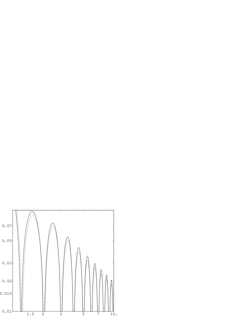
FIG. 13.: As in Fig. 12, but only for $\alpha=1$ with $\lambda=1$. The full line shows the solution through order $\lambda^{3/2}$ and the dotted line the Padé improved solution.

VI Conclusion

We have studied the effects of weak self-interactions in an ultrarelativistic plasma on cosmological perturbations through order $\lambda^{3/2}$ in $\lambda\phi^{4}$-theory. At this order it turns out that perturbation theory requires a resummation of an infinite set of higher-order diagrams. This is natural to include in the thermal-field-theory approach to cosmological perturbations, which in the collisionless case is equivalent to the usual approach based on classical kinetic theory, but now leaves the latter clearly behind.

While it still turned out to be possible to exactly solve the perturbation equations by means of a power series ansatz, we have found that the relatively large coefficients of the order-$\lambda^{3/2}$ corrections make the results reliable only for rather small values of $\lambda$, and even then there is a breakdown of perturbation theory in the asymptotic late-time behaviour. The latter comes from increasingly singular contributions to the gravitational polarization tensor for light-like momenta and could be cured by a further resummation procedure. However, the effects of the latter turned out to be well approximated by a (2,1)-Padé-improvement of the perturbative results, which also drastically improves the apparent convergence of the results for smaller times.

The concrete results obtained showed a tendency toward perfect-fluid behaviour, but with $\lambda=1$ all of them are still (perhaps surprisingly) close to the collisionless case. The main effects turned out to be a small increase of the critical mixing factor of a perfect-fluid component with a relativistic plasma above which one can have singular solutions exhibiting superhorizon oscillations. Concerning the regular solutions, we have found a decrease of the phase velocity of scalar perturbations and a reduction of its damping. In the case of vector perturbations (corresponding to large-scale vorticity), which are only possible in the presence of a relativistic plasma, similar effects were found, but quantitatively much smaller. Very little effects from self-interactions were finally observed in the case of tensor perturbations, which correspond to primordial gravitational waves.

From this one may conclude that a description of a primordial plasma built from weakly interacting elementary particles through perfect-fluid models is in general applicable only for scales far below the Hubble radius. At the scale of the horizon and beyond, self-interactions can be treated perturbatively, at least in the model considered here, and there can be significant differences from the perfect-fluid behaviour, in particular in the case of rotational perturbations.

A Gravitational polarisation tensor components and its Fourier transforms

The Fourier transform of the combinations of the gravitational polarisation tensor components [19]

$$A = -\omega\,{\rm artanh}{1\over\omega}+\frac{5}{4}$$ (A1)

$$- {5\lambda\over 8\pi^{2}}\left[2\left(\omega\,{\rm artanh}{1\over\omega}\right)^{2}-\omega\,{\rm artanh}{1\over\omega}-{\omega^{2}\over{\omega^{2}-1}}\right]$$ (A2)

$$- {5\lambda^{3/2}\over 8\pi^{3}}\biggl{[}3\left({\omega^{2}-1}-\omega\sqrt{\omega^{2}-1}\right)\left(\omega\,{\rm artanh}{1\over\omega}\right)^{2}$$ (A5)

$$+6\left(\omega\sqrt{\omega^{2}-1}-\omega^{2}-{\omega\over\sqrt{\omega^{2}-1}}\right)\omega\,{\rm artanh}{1\over\omega}$$

$$+{\omega\over({\omega^{2}-1})^{3/2}}+3{\omega^{2}\over{\omega^{2}-1}}+6{\omega\over\sqrt{\omega^{2}-1}}-3\omega\sqrt{\omega^{2}-1}+3\omega^{2}\biggr{]},$$

$$B = -1+{5\lambda\over 4\pi^{2}}\left[-({\omega^{2}-1})\left(\omega\,{\rm artanh}{1\over\omega}\right)^{2}+(2\omega^{2}-1)\omega\,{\rm artanh}{1\over\omega}-\omega^{2}\right]$$ (A6)

$$+ {15\lambda^{3/2}\over 8\pi^{3}}\biggl{[}\left\{\omega({\omega^{2}-1})^{3/2}-({\omega^{2}-1})^{2}\right\}\left(\omega\,{\rm artanh}{1\over\omega}\right)^{2}$$ (A9)

$$+2\left\{({\omega^{2}-1})^{2}-\omega({\omega^{2}-1})^{3/2}+\omega\sqrt{\omega^{2}-1}-\omega^{2}\right\}\omega\,{\rm artanh}{1\over\omega}$$

$$-{\omega\over\sqrt{\omega^{2}-1}}-2\omega\sqrt{\omega^{2}-1}+\omega({\omega^{2}-1})^{3/2}-\omega^{4}+4\omega^{2}\biggr{]},$$

$$C = -{5\lambda\over 8\pi^{2}}\left[3({\omega^{2}-1})^{2}\left(\omega\,{\rm artanh}{1\over\omega}\right)^{2}-2({\omega^{2}-1})(3\omega^{2}-2)\omega\,{\rm artanh}{1\over\omega}+3\omega^{4}-4\omega^{2}\right]$$ (A10)

$$- {15\lambda^{3/2}\over 16\pi^{3}}\biggl{[}3({\omega^{2}-1})^{2}\left({\omega^{2}-1}-\omega\sqrt{\omega^{2}-1}\right)\left(\omega\,{\rm artanh}{1\over\omega}\right)^{2}$$ (A13)

$$-2({\omega^{2}-1})\left\{3({\omega^{2}-1})^{2}-3\omega({\omega^{2}-1})^{3/2}+3\omega\sqrt{\omega^{2}-1}-3\omega^{2}+1\right\}\omega\,{\rm artanh}{1\over\omega}$$

$$-3\omega({\omega^{2}-1})^{5/2}+6\omega({\omega^{2}-1})^{3/2}+\omega\sqrt{\omega^{2}-1}+3\omega^{6}-15\omega^{4}+16\omega^{2}\biggr{]},$$

with powers of $\omega$, as required in (III A 1,43,47), boils down to the evaluation of the following integrals

$$\int_{-1}^{1}{d\omega\over\pi}\cos(\omega x)(1-\omega^{2})^{\beta-\frac{1}{2}}=\left(\frac{2}{x}\right)^{\beta}\frac{\Gamma(\beta+\frac{1}{2})}{\sqrt{\pi}}J_{\beta}(x),$$ (A14)

$$\frac{1}{2}\int_{-1}^{1}d\omega\sin(\omega x)\ln{1+\omega\over 1-\omega}={1\over x}\left[\sin(x){\rm Si}(2x)+\cos(x)\left({\rm Ci}(2x)-\gamma-\ln(2x)\right)\right]$$ (A15)

$$=2\sum_{m=0}^{\infty}{(-1)^{m}x^{2m+1}\over(2m+2)!}\sum_{j=0}^{m}{1\over 2j+1}=:\kappa(x),$$ (A16)

$$\int_{-1}^{1}{d\omega\over 2\pi}\cos(\omega x){\omega\over\sqrt{1-\omega^{2}}}\ln{1+\omega\over 1-\omega}=:\nu(x),$$ (A17)

$$-12\int_{-1}^{1}{d\omega\over 2\pi}\cos(\omega x)\sqrt{1-\omega^{2}}\left({\omega\over 2}\ln{1+\omega\over 1-\omega}\right)^{2}-{3\pi^{2}\over 2}\left(J_{1}\over x\right)^{\prime\prime}=:\xi(x)$$ (A18)

where additional powers of $\omega$ in the integrands can be obtained by suitably differentiating those functions with respect to $x$. Let us first consider a typical integral appearing in the power-series expansion in $x$ of $\nu(x)$,

$$S_{m}=\int_{-1}^{1}d\omega\frac{\omega^{2m+1}}{\sqrt{1-\omega^{2}}}\ln\frac{1+\omega}{1-\omega}.$$

By integration by parts with respect to the root, it can be shown to satisfy the recursion $S_{m}=2m(S_{m-1}-S_{m})+2\sqrt{\pi}\Gamma(\frac{1}{2}+m)/m!$ which may be solved for $S_{m}$,

$$S_{m}=2\sqrt{\pi}\sum_{l=0}^{n}\frac{\Gamma(\frac{1}{2}+l)}{l!(1+2m-2l)},$$

that finally leads to the expression

$$\nu(x) = \sum_{m=0}^{\infty}{(-1)^{m}x^{2m}\over(2m)!}\sum_{l=0}^{m}{\Gamma(l+\frac{1}{2})\over\sqrt{\pi}l!(1+2m-2l)}.$$ (A19)

The square of the logarithm in the more complicated power-series coefficients of $\xi(x)$,

$$T_{m}=\int_{-1}^{1}d\omega\omega^{2m+2}\sqrt{1-\omega^{2}}\ln^{2}\frac{1+\omega}{1-\omega},$$

can be removed by integrating by parts in the same manner as above with the remaining integral being of the type of $S_{m}$ with the root in the numerator. $T_{m}$ satisfies the recursion $3T_{m}=(2m+1)(T_{m-1}-T_{m})+4(S_{m}-S_{m+2})$ which can be solved using the initial integral $T_{0}=\pi^{3}/8-2\pi/3$. Splitting off the contributions $\propto\pi^{3}$ which can be reexpressed in terms of $J_{1}(x)$ finally yields

$$\xi(x)=6\sum_{m=0}^{\infty}{(-1)^{m}x^{2m}\over(2m)!}{\Gamma(m+\frac{3}{2})\over\Gamma(\frac{1}{2})\Gamma(m+3)}\left(1-\sum_{l=0}^{m}{\Gamma(l+1)\over 4\Gamma(l+\frac{3}{2})}\sum_{j=0}^{l}{\Gamma(j+\frac{1}{2})\over j!(l-j+\frac{3}{2})}\right)\ .$$ (A20)

B Recursion relations

In order to solve the integro-differential equations for the metric potentials a power series ansatz is appropriate. The integral kernels are expanded as

$$K^{(a)}(x)=\sum_{n=0}^{\infty}(-1)^{n}K^{(a)}_{n}{x^{2n}\over(2n)!}\ .$$ (B1)

They read:

$$K^{(0)}_{n} = {1\over 2n+1}+\frac{5}{8}{\lambda\over\pi^{2}}\left({2\over n+1}\sum_{j=0}^{n}{1\over 2j+1}-1-{1\over 2n+1}\right)+$$ (B6)

$$+\frac{15}{8}\left({\lambda\over\pi^{2}}\right)^{\frac{3}{2}}\left[1+{(2n-1)!!\over(2n-2)!!}\left({1\over 3}+{1\over n}+{1\over 2n(2n+2)}\right)-{6\over 2n+3}-\right.$$

$$\qquad-{1\over(n+1)(n+2)}\sum_{j=0}^{n}{1\over 2j+1}+{1\over(n+2)(2n+3)}-$$

$$\qquad-{4\over\sqrt{\pi}}\sum_{j=0}^{n}{\Gamma(j+\frac{1}{2})\over j!(2n-2j+1)}+{2\over\sqrt{\pi}}\sum_{j=0}^{n+1}{\Gamma(j+\frac{1}{2})\over j!(2n-2j+3)}-$$

$$\qquad\left.-{\Gamma(n+\frac{3}{2})\over\sqrt{\pi}(n+2)!}\left(1-\sum_{l=0}^{n}{l!\over 2\Gamma(l+\frac{3}{2})}\sum_{j=0}^{l}{\Gamma(j+\frac{1}{2})\over j!(2l-2j+3)}\right)\right]\,$$

$$K^{(1)}_{n} = -{1\over(2n+1)(2n+3)}+\frac{5}{4}{\lambda\over\pi^{2}}{n\over(2n+1)(2n+3)}-$$ (B8)

$$-\frac{5}{8}\left({\lambda\over\pi^{2}}\right)^{\frac{3}{2}}\left({(2n-1)!!\over(2n)!!}-{1\over 2n+1}+{8n\over(2n+1)(2n+3)}\right)\ ,$$

$$K^{(2)}_{n} = -{8\over(2n+1)(2n+3)(2n+5)}+5{\lambda\over\pi^{2}}{1\over(2n+1)(2n+3)}\left(1-{3\over 2n+5}\right)-$$ (B10)

$$-5\left({\lambda\over\pi^{2}}\right)^{\frac{3}{2}}\left[{(2n-1)!!\over(2n+2)!!}+{3\over(2n+1)(2n+3)}\left(1-{4\over 2n+5}\right)\right]\ .$$

In this Appendix we restrict our attention to regular even solutions, as the kernels are even functions of $x$. This means that we assume $\gamma_{2n+1}^{(a)}=0$ for all $n$ and $a$. Regular odd and singular solutions may be obtained in a similar way [16].

1 Scalar Perturbations

With

$$\Phi_{N}=\sum_{n=0}^{\infty}(-1)^{n}\phi_{n}{x^{2n}\over(2n)!}$$ (B11)

Eq. (58) leads to the recursion relation

$$\left[6n+9-{9\alpha\over n+1}\left(K_{1}^{(0)}-3K_{2}^{(0)}\right)\right]\phi_{n} = -4\sum_{l=1}^{n-1}(l+2)\phi_{l}+$$ (B12)

$$+ {9\alpha\over n+1}\sum_{l=1}^{n-1}\left(K_{l+1}^{(0)}-3K_{l+2}^{(0)}\right)\phi_{n-l}+$$ (B13)

$$+ {9\alpha\over n+1}\sum_{l=0}^{\infty}(-1)^{l}\gamma_{2l}^{(0)}\left(K_{n+1+l}^{(0)}-3K_{n+2+l}^{(0)}\right)+$$ (B14)

$$+ \phi_{0}-9\alpha\sum_{l=0}^{\infty}(-1)^{l}\gamma_{2l}^{(0)}\left(K_{1+l}^{(0)}-3K_{2+l}^{(0)}\right)\ ,$$ (B15)

for $n\geq 1$. The regularity at $x=0$ demands

$$\phi_{0}=C_{1}+\frac{2}{3}\sum_{l=0}^{\infty}\gamma_{2l}(-1)^{l}(2n-4)\ .$$ (B16)

Accordingly, the metric perturbation

$$\Pi=\sum_{n=0}^{\infty}(-1)^{n}\pi_{n}{x^{2n}\over(2n)!}$$ (B17)

is determined from Eqs. (13) and (39). Its recursion reads:

$$\pi_{n} = {3\alpha\over(n+1)(2n+1)}\left[\sum_{l=1}^{n}\left(K^{(0)}_{l}-3K^{(0)}_{l+1}\right)\phi_{n-l+1}+\right.$$ (B19)

$$\left.+\sum_{l=0}^{\infty}\gamma_{2l}(-1)^{l}\left(K^{(0)}_{n+l+1}-3K^{(0)}_{n+l+2}\right)\right]$$

for $n\geq 0$. The relativistic plasma component perturbation

$$\Phi_{\rm RP}=\sum_{n=0}^{\infty}(-1)^{n}q_{n}{x^{2n}\over(2n)!}$$ (B20)

follows from (61) and reads

$$q_{n} = {3\alpha\over(n+1)(2n+1)}\left[-\phi_{n+1}-\pi_{n+1}+2\sum_{l=0}^{n}\left(K^{(0)}_{l}+{3\over 2n+3}K^{(0)}_{l+1}\right)\phi_{n-l+1}+\right.$$ (B22)

$$\left.+2\sum_{l=0}^{\infty}\gamma_{2l}(-1)^{l}\left(K^{(0)}_{n+l+1}+{3\over 2n+3}K^{(0)}_{n+l+2}\right)\right]$$

for $n\geq 0$. From regularity at $x=0$

$$C_{1}=\sum_{l=0}^{\infty}\gamma_{2l}(-1)^{l}\left(-\frac{2}{3}(2l-4)+9\alpha K^{(0)}_{l+2}-3(\alpha-2)K^{(0)}_{l+1}+2K^{(0)}_{l}\right)$$ (B23)

follows.

2 Vector Perturbations

The vector metric potential

$$\Psi=\sum_{n=0}^{\infty}(-1)^{n}\psi_{n}{x^{2n}\over(2n)!}$$ (B24)

is determined by the Eqs. (19) and (46). The corresponding recursion is

$$\left[(n+1)(2n+1)-12\alpha K_{1}^{(1)}\right]\psi_{n} = 12\alpha\sum_{l=1}^{n}K_{l+1}^{(1)}\psi_{n-l}+$$ (B25)

$$+ 12\alpha\sum_{l=0}^{\infty}(-1)^{l}\gamma_{2l}^{(1)}K_{n+1+l}^{(1)}\ ,$$ (B26)

for $n\geq 0$. The relation (63) couples the vorticity of the perfect fluid component to the coefficients $\gamma_{2l}^{(1)}$.

3 Tensor Perturbations

For the metric potential $H$ the ansatz

$$H=\sum_{n=0}^{\infty}(-1)^{n}h_{n}{x^{2n}\over(2n)!}$$ (B27)

is made. Regular even solutions follow from Eqs. (21) and (47) by

$$\left[(2n+1)2n-3\alpha K_{0}^{(2)}\right]h_{n} = 2n(2n-1)h_{n-1}+3\alpha\sum_{l=1}^{n-1}K_{l}^{(2)}h_{n-l}+$$ (B28)

$$+ 3\alpha\sum_{l=0}^{\infty}(-1)^{l}\gamma_{2l}^{(2)}K_{n+l}^{(2)}$$ (B29)

for $n\geq 1$. The initial value $h_{0}$ specifies together with the inhomogeneous terms the regular solution.

REFERENCES

• [1] E. Lifshitz, Zh. Eksp. Teor. Fiz. 16, 587 (1946); E. Lifshitz and I. Khalatnikov, Adv. Phys. 12, 185 (1963).
• [2] H. Kodama and M. Sasaki, Prog. Theor. Phys. Suppl. 78, 1 (1984).
• [3] V. F. Mukhanov, H. A. Feldman, and R. H. Brandenberger, Phys. Rep. 215, 203 (1992); R. Durrer, Gauge Invariant Cosmological Perturbation Theory, Report No. ZU-TH14/92, 1993.
• [4] P. J. E. Peebles and J. T. Yu, Astrophys. J. 162, 815 (1970).
• [5] A. I. McCone, Ph. D. thesis, Univ. of Maryland, Tech. Rept. UMD-70-054 (1970).
• [6] P. J. E. Peebles, Astrophys. J. 180, 1 (1973).
• [7] J. R. Bond and A. S. Szalay, Astrophys. J. 274, 443 (1983).
• [8] J. Ehlers, in General Relativity and Gravitation, edited by R. K. Sachs (Academic Press, New York, 1971); J. M. Stewart, Non-equilibrium Relativistic Kinetic Theory, (Springer-Verlag, New York, 1971).
• [9] J. M. Stewart, Astrophys. J. 176, 323 (1972).
• [10] A. V. Zakharov, Sov. Phys. JETP 50, 221 (1979); E. T. Vishniac, Astrophys. J. 257, 456 (1982).
• [11] U. Kraemmer and A. Rebhan, Phys. Rev. Lett. 67, 793 (1991).
• [12] A. Rebhan, Nucl. Phys. B351, 706 (1991).
• [13] J. Frenkel and J. C. Taylor, Z. Phys. C 49, 515 (1991); F. T. Brandt, J. Frenkel and J. C. Taylor, Nucl. Phys. B374, 169 (1992); A. P. de Almeida, F. T. Brandt and J. Frenkel, Phys. Rev. D 49, 4196 (1994); J. Frenkel, E. A. Gaffney and J. C. Taylor, Nucl. Phys. B439, 131 (1995).
• [14] A. Rebhan, Nucl. Phys. B368, 479 (1992);
• [15] D. J. Schwarz, Int. J. Mod. Phys. D 3, 265 (1994).
• [16] A. K. Rebhan and D. J. Schwarz, Phys. Rev. D 50, 2541 (1994).
• [17] M. Kasai and K. Tomita, Phys. Rev. D 33, 1576 (1986).
• [18] H. Nachbagauer, A. K. Rebhan, and D. J. Schwarz, Phys. Rev. D 51, R2504 (1995).
• [19] H. Nachbagauer, A. K. Rebhan, and D. J. Schwarz, The gravitational polarization tensor of thermal $\lambda\phi^{4}$ theory, preprint hep-th/9507099 (1995).
• [20] J. M. Bardeen, Phys. Rev. D 22, 1882 (1980).
• [21] J. I. Kapusta, Finite-temperature field theory, (Cambridge University Press, Cambridge, 1989); M. Le Bellac, Thermal Field Theory to appear in Cambridge University Press.
• [22] E. Braaten and R. D. Pisarski, Nucl. Phys. B355, 1 (1991).
• [23] M. Bruni, P. K. S. Dunsby, and G. F. R. Ellis, Astrophy. J. 395, 34 (1992).
• [24] L. P. Grishchuk, Phys. Rev. D 50, 7154 (1994).
• [25] N. Deruelle and V. F. Mukhanov, On matching conditions for cosmological perturbations, gr-qc/9503050 (1995).
• [26] R. K. Schaefer and A. A. de Laix, Gauge invariant density and temperature perturbations in the quasi-Newtonian formulation, astro-ph/9507003 (1995).
• [27] A. Rebhan, Astrophys. J. 392, 385 (1992).
• [28] S. Wolfram, Mathematica 2nd Ed., (Addison-Wesley, Redwood City, 1991).
• [29] G. Bรถrner, The Early Universe: Facts and Fiction (Springer, Berlin, 1993).
• [30] L. Dolan and R. Jackiw, Phys. Rev. D 9, 3320 (1974).
• [31] G.ย A.ย Baker, Jr., Essentials of Padรฉ Approximants, (Academic Press, New York, 1975).
• [32] B. Davies, Integral Transforms and Their Applications, (Springer-Verlag, New York, 1978).
• [33] B. J. T. Jones, Rev. Mod. Phys. 48, 107 (1976).