Cauchy Problem for Gott Spacetime

Gott recently has constructed a spacetime modeled by two infinitely long, parallel cosmic strings which pass and gravitationally interact with each other. For large enough velocity, the spacetime will contain closed timelike curves. An explicit construction of the solution for a scalar field is presented in detail and a proof for the existence of such a solution is given for initial data satisfying conditions on an asymptotically null partial Cauchy surface.

Solutions to smooth operators on the covering space are invariant under the isometry are shown to be pull back of solutions of the associated operator on the base space.

Projection maps and translation operators for the covering space are developed for the spacetime, and explicit expressions for the projection operator and the isometry group of the covering space are given. It is shown that the Gott spacetime defined is a quotient space of Minkowski space by the discrete isometry subgroup of self-equivalences of the projection map.

Contents

toc

I Introduction

The question of the validity of spacetimes with closed timelike curves has been studied for several decades by many authors. See [2, 4] for a the state of the art review. It is not a simple task to determine whether closed timelike curves (CTC’s) are allowed in nature. It has been shown that solutions in some nonchronal spacetimes are exist for data on certain initial value surfaces [6, 7].

Gott has obtained a family of exact solution to Einstein’s equations describing a system of two straight, infinitely long cosmic strings [12]. The resultant spacetime is flat except at conical singularities representing the string loci. The important feature of this spacetime is that, for sufficiently high relative velocity, it contains CTC’s [11]. Its global structure has been studied, and the region containing CTC’s has been determined [15].

The question of whether or not a solution to fields that exist in the Gott spacetimes is not in general known. The purpose of this work is to show that for the scalar wave equation on a particular Gott spacetime, asymptotically well behaved data gives a solution everywhere except possibly at the string loci.

The organization of the work is as follows. In II, we outline the Gott two-string spacetime, (M,g). In section III, we discuss the covering space for M and how it relates to the general solution for the massless wave equation and the initial data surface. Section IV gives a formal proof that the Gott spacetime is covered by Minkowski space. Sections V and VI detail some of the important symmetries of of the spacetime. Finally, section VII gives a general form for the scalar field in terms of angular quadratures with the theorem and proof that the integrals obtained are indeed defined and well behaved. We discuss miscellaneous details in the appendices.

II The Gott Spacetime

In $2+1$ dimensions, the general vacuum solution to Einstein’s equation with a point mass is flat except for a conical singularities at the location of the masses. In $3+1$ dimensions, there are corresponding solutions with singularities on the worldsheets of the strings. The mass (mass per length ${{}\mu}$ in the $3+1$ case) is proportional to the deficit angle of the conical singularity [12].

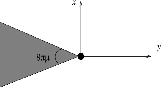
FIG. 1.: The spacetime wedge cut out by a cosmic string. The deficit angle is given by $8\pi{{}\mu}$, where $\mu$ is the mass per unit length of the string.

Two relatively moving strings, with their corresponding deficit angles, will produce close timelike curves. If the sum of the deficit angles is less than or equal to $\pi$, the resultant spacetime will be open in the topological sense [10]. The case where the deficit angles are equal and sum to $\pi$ is considered in the work. This will be essential in order that Minkowski space be a covering space of the physical space.

Let the two strings parallel to the $z$ axis be located at $x=0,y=\pm Y_{0}$ at $t=0$. In a static situation, we identify the $-x$ and $x$ components of each string. The spacetime can thus be viewed as a $3+1$ slab with $-Y_{0}\leq y\leq Y_{0}$ that has been identified in the prior fashion.

In the dynamic case, the two strings are moving relative to one another in $y$ as in figure 2 and the identifications are Lorentz transformations of the static case.

FIG. 2.: The Gott spacetime as viewed along the string axis. The top string is moving to the left and the bottom string moves to the right. The hash marks indicate identification along the lines $y=\pm Y_{0}$.

Define null coordinates $x_{\pm}=x\pm t$ on Minkowski spacetime. It will be shown that the Lorentz boosted identifications for the 2 string system are

$$\begin{array}[]{c}x^{\pm}\to e^{\mp{{}\alpha}}x^{\mp}\quad(y=+Y_{0})\cr x^{\pm}\to e^{\pm{{}\alpha}}x^{\mp}\quad(y=-Y_{0})\cr A_{+}:x^{\pm}\doteq-e^{\mp 2{{}\alpha}}x^{\mp}\quad(y=+Y_{0})\cr A_{-}:x^{\pm}\doteq-e^{\pm 2{{}\alpha}}x^{\mp}\quad(y=-Y_{0})\cr\end{array}$$ (1)

where $A_{\pm}$ are the identification maps at $\pm Y_{0}$.

III Covering Space for Gott Spacetime

The proceeding section suggests that Gott Spacetime can be covered by Minkowski spacetime. This will be demonstrated directly in section III A. Define the unit cell $D_{o}$ as the spacetime slab bounded by the planes $y=\pm Y_{0}$. Similarly, define the n-cell $D_{n}$ as

$$D_{n}=\biggl{\{}{{}\widetilde{\bf x}}\in{{}\widetilde{\hbox{\rm M}}}\big{|}(2n-1)Y_{0}<y<(2n+1)Y_{0}\biggr{\}}.$$ (2)

Gott spacetime can be characterized by the space $D_{o}$ with the boundaries $y=\pm Y_{0}$ identified by the relations 1. We proceed to develop the explicit covering maps and other terminology needed.

A Projection Maps for Stationary Strings

In this section, the projection map for the covering space is developed by following a trajectory in Minkowski spacetime. The static case is considered first, and afterwards, the dynamic case which contains CTC’s is discussed. The two spaces are topologically equivalent.

The covering map for the stationary case follow from the fact that when one crosses any boundary $y=(2n+1)Y_{0}$, the identifications (1) reflect through an angle of $\pi$ about the point $x=0$.

We can deduce the projection maps in the static case by simply following a trajectory that moves vertically up in the $y$ direction as in figure 3.

1. For $-Y_{0}\leq y\leq Y_{0}$ $\pi$ is the identity:

$$\pi(x,y,z)=(x,y,z)$$ (3)

2. For $Y_{0}\leq y\leq 3Y_{0}$: $x\longrightarrow-x\;;\;y\longrightarrow Y_{0}-{{}\Delta}\equiv Y_{0}-(y-Y_{0})=2Y_{0}-y$ where ${{}\Delta}$ is defined as the extra difference between the nearest line $y=(2n+1)Y_{0}$ and the point in the path. Hence,

$$\pi(x,y,z)=(-x,2Y_{0}-y,z)$$ (4)

3. For $3Y_{0}\leq y\leq 5Y_{0}$, $x\longrightarrow x\;;\;y\longrightarrow-Y_{0}+{{}\Delta}=-Y_{0}+(y-3Y_{0})=y-4Y_{0}$,

and so

$$\pi(x,y,z)=(x,y-4Y_{0},z).$$ (5)

One can generalize the maps in the expression:

For $(2n-1)Y_{0}\leq y\leq(2n+1)Y_{0}$  ,

$$\pi(x,y,z)=((-1)^{n}x,(-1)^{n}(y-2nY_{0}),z)\;,\;\quad\forall x\in D_{n}$$ (6)

FIG. 3.: A path in the covering space to determine the projection map $\pi$. The dotted vertical line in ${\widetilde{\hbox{\rm M}}}$ represents the path in the covering space that become the vertical paths in M.

B Projection Maps for Boosted Strings

The null ${{\tilde{x}}}$ coordinates in the stationary frame defined by

$${{\tilde{x}}}^{+}={{\tilde{x}}}+{{\tilde{t}}}\quad;\quad{{\tilde{x}}}^{-}={{\tilde{x}}}-{{\tilde{t}}}$$ (7)

are used. Under a the lorentz transformation for the lower string at $y=-Y_{0}$ moving in the $+x$ direction,

$$x^{\pm}=e^{\pm{{}\alpha}}{{\tilde{x}}}^{\pm}\quad;\quad y={{\tilde{y}}}-Y_{0}$$ (8)

where the ${{\tilde{x}}}$ coordinates are stationary w.r.t. the point mass (string). We identify antipodal (in ${{\tilde{x}}}$) points at $y=-Y_{0}$ using $A_{-}$ we obtain

$$A_{-}{{\tilde{x}}}=-{{\tilde{x}}}{{}\;\Rightarrow\;}A_{-}e^{-{{}\alpha}}x^{+}=-e^{{{}\alpha}}x^{-}{{}\;\Rightarrow\;}A_{-}x^{\pm}=-e^{2{{}\alpha}}x^{\mp}.$$ (9)

or equivalently,

$$A_{-}:x^{\pm}\longmapsto-e^{\pm 2{{}\alpha}}x^{\mp}\quad(y=-Y_{0})$$ (10)

Translating (10) back to $(x,t)$ coordinates,

$$\begin{array}[]{ccc}A_{-}:x\longmapsto-x\cosh 2{{}\alpha}+t\sinh 2{{}\alpha}\cr A_{-}:t\longmapsto-x\sinh 2{{}\alpha}+t\cosh 2{{}\alpha}\cr\end{array}\qquad(y=-Y_{0})$$ (11)

For the second point mass at $y=Y_{0}$ moving in the $+{{\hat{x}}}$ direction,

$$\begin{array}[]{lll}A_{+}:x^{\pm}\!\longmapsto-e^{\mp 2{{}\alpha}}{{\tilde{x}}}^{\mp}\cr A_{+}:x\;\longmapsto-x\cosh 2{{}\alpha}-t\sinh 2{{}\alpha}\cr A_{+}:t\;\longmapsto+x\sinh 2{{}\alpha}+t\cosh 2{{}\alpha}\cr\end{array}\qquad(y=Y_{0})$$ (12)

We are now in a position to define our Gott spacetime. Define a three dimensional spacelike slab, $W_{0}=[-Y_{0},Y_{0}]\times R^{2}$. Let $S_{0}=R\times W_{0}$ where the copy of $R$ corresponds to time $t$. The Gott spacetime M is defined by $S_{0}$ with identifications $A_{\pm}$ given by

$$A_{\pm}:(x^{+},x^{-},Y_{0},z)\longmapsto(-e^{\mp 2{{}\alpha}}x^{-},-e^{\pm 2{{}\alpha}}x^{+},Y_{0},z)\quad@\quad y=\pm Y_{0}$$ (13)

The action of the projections can be found by following the coordinates in the base space sequentially through a path from $y=0$ to $y=2Y_{0}$ in the covering space.

$$\begin{array}[]{ccccc}0&\quad\longrightarrow&\quad Y_{0}&\quad\longrightarrow&\quad 3Y_{0}\cr x^{+}&\quad\longrightarrow&\quad-e^{-2{{}\alpha}}x^{-}&\quad\longrightarrow&\quad-e^{+2{{}\alpha}}(-e^{+2{{}\alpha}}x^{+})\cr x^{-}&\quad\longrightarrow&\quad-e^{+2{{}\alpha}}x^{+}&\quad\longrightarrow&\quad-e^{-2{{}\alpha}}(-e^{-2{{}\alpha}}x^{-})\cr y&\quad\longrightarrow&\quad y-2Y_{0}&\quad\longrightarrow&\quad 4Y-0-y\end{array}$$ (14)

1. For $-Y_{0}\leq y\leq Y_{0}$ we again have the identity map;

$$\pi(x^{+},x^{-},y)=(x^{+},x^{-},y).$$ (15)

2. For $Y_{0}\leq y\leq 3Y_{0}$:

$$\pi(x^{+},x^{-},y)=(-e^{-2{{}\alpha}}x^{-},-e^{+2{{}\alpha}}x^{+},2Y_{0}-y)=K^{-1}PL^{-1}(x^{+},x^{-},y)$$ (16)

3. For $3Y_{0}\leq y\leq 5Y_{0}$:

$$\pi(x^{\pm},y)=(e^{+4{{}\alpha}}x^{+},e^{-4{{}\alpha}}x^{-},y-4Y_{0})=KPLK^{-1}PL^{-1}(x^{+},x^{-},y)$$ (17)

where $P$ is defined as the spatial parity operator, $K$ is the Lorentz boost operator in $\hat{x}$ with velocity $\tanh{{}\alpha}$, and $L$ ($L^{-1}$) is translation in $\hat{y}$ by $2Y_{0}$ ($-2Y_{0}$). The first two operators are defined as

$$\begin{array}[]{c}K(x^{+},x^{-},y)=(e^{-2{{}\alpha}}x^{+},e^{+2{{}\alpha}}x^{-},y)\cr K^{n}(x^{+},x^{-},y)=(e^{-2n{{}\alpha}}x^{+},e^{+2n{{}\alpha}}x^{-},y)\cr P(x^{+},x^{-},y)=(-x^{-},-x^{+},-y)\cr P^{n}(x^{+},x^{-},y)=(-1)^{n}(x^{(-)^{n}},x^{(-)^{n+1}},y)\cr\end{array}$$ (18)

In the $(x^{+},x^{-},y)$ basis, $K$ and $P$ can be written as matrices:

$$K=\left[\begin{array}[]{ccc}e^{2{{}\alpha}}&\ 0&\ 0\cr\ 0&e^{-2{{}\alpha}}&0\cr 0&0&1\cr\end{array}\right]\qquad P=\left[\begin{array}[]{ccc}\ 0&-1&\ 0\cr-1&\ \ 0&\ 0\cr 0&\ \ 0&-1\cr\end{array}\right]$$ (19)

A few properties of $K^{n}$, $P^{n}$, and $L^{n}$ should be noted.

$$\begin{array}[]{c}[K^{n},L^{m}]=0\cr PL=L^{-1}P\quad;\quad P^{n}L^{m}=L^{(-1)^{n}m}=L^{\hbox{$s_{nm}$}}\cr K^{n}P=PK^{-n}\quad;\quad K^{n}P^{n}=P^{n}K^{\hbox{$s_{n}$}}\cr\end{array}$$ (20)

where $s_{n}\equiv(-1)^{n}n$, $s_{nm}\equiv(-1)^{n}m$, and

$$K^{\hbox{$s_{n}$}}=\left(\begin{array}[]{ccc}e^{2{\hbox{$s_{n}$}}{{}\alpha}}&\ 0&\ 0\cr\ 0&e^{-2\hbox{$s_{n}$}{{}\alpha}}&0\cr 0&0&1\cr\end{array}\right)$$ (21)

From the above expressions, it follows that

$$KPLK^{-1}PL^{-1}=K^{2}P^{2}L^{-2}=K^{2}L^{-2}$$ (22)

Thus the restriction $\pi_{n}$ of $\pi$ to $D_{n}$ where $(2n-1)Y_{0}\leq y\leq(2n+1)Y_{0}$  , had the form

$$\pi_{n}(x^{+},x^{-},y)=K^{\hbox{$s_{n}$}}P^{n}L^{-n}(x^{+},x^{-},y),$$ (23)

where we are regarding M as the $O^{\hbox{th}}$-cell $D_{o}$ of Eq. (2) withe identifications (1).

Let’s check against the result of Boulware [11] for the set of equivalent points $\pi^{-1}$. First, note that for $n=1$,

$$\begin{array}[]{cl}\pi_{1}(x^{+},x^{-},y)&=K^{-1}PL(x^{+},x^{-},y)\cr&=\left(\begin{array}[]{ccc}e^{-2{{}\alpha}}&\ 0&\ 0\cr\ 0&e^{+2{{}\alpha}}&0\cr 0&0&1\cr\end{array}\right)\left(\begin{array}[]{c}-x^{-}\cr-x^{+}\cr 2Y_{0}-y\cr\end{array}\right)=\left(\begin{array}[]{c}-e^{-2{{}\alpha}}x^{-}\cr-e^{+2{{}\alpha}}x^{+}\cr 2Y_{0}-y\cr\end{array}\right)\cr\end{array}$$ (24)

This is equation (2.8) of reference [11]. Next let $n=-1$

$$\pi_{-1}{{\bf x}}=KPL^{-1}{{\bf x}}=\left(\begin{array}[]{ccc}e^{+2{{}\alpha}}&\ 0&\ 0\cr\ 0&e^{-2{{}\alpha}}&0\cr 0&0&1\cr\end{array}\right)\left(\begin{array}[]{c}-x^{-}\cr-x^{+}\cr{\scriptstyle-y-2Y_{0}}\cr\end{array}\right)=\left(\begin{array}[]{c}-e^{+2{{}\alpha}}x^{-}\cr-e^{-2{{}\alpha}}x^{+}\cr{\scriptstyle-y-2Y_{0}}\cr\end{array}\right)$$ (25)

which is equation (2.6) of [11]. Note that in the static case ($e^{\pm 2n{{}\alpha}}\to 1$), $\pi$ can be rewritten as

$$\pi_{n}(x^{+},x^{-},y)=P^{n}L^{-n}(x^{+},x^{-},y).$$ (26)

which is the correct limiting form.

IV Theorem for the Covering Space

Theorem 1

Let ${\widetilde{\hbox{\rm M}}}$ be Minkowski spacetime with the string worldsheets removed, and let ${{}\pi}:{{}\widetilde{\hbox{\rm M}}}\longrightarrow{}{\hbox{\rm M}}$ be defined as above. Then ${\widetilde{\hbox{\rm M}}}$ is a covering space of M and ${{}\pi}:{{}\widetilde{\hbox{\rm M}}}\longrightarrow{}{\hbox{\rm M}}$ is the projection map.

We prove the theorem with the following

Claim 1

$\pi$ is a local homeomorphism in the static case.

Proof:

Take a point ${\bar{e}}=(\bar{e}_{x},\bar{e}_{y})$ that lies interior to all lines $y=(2n+1)Y_{0}$ such that ${{}\pi}({\bar{e}})=e$. Then there is an open nbhd $U_{\bar{e}}$ such that

$$U_{\bar{e}}=\{(x,y)\in{{}\widetilde{\hbox{\rm M}}}\Bigm{|}|(x,y)-({\bar{e}}_{x},{\bar{e}}_{y})|<\min(|(x,y)-(x,(2n+1)Y_{0})|)\forall n\}$$ (27)

Then ${{}\pi}(U_{\bar{e}})$ is mapped homeomorphically onto an open set $V_{e}$ since $\pi$ is a polynomial map of degree one, which is continuous and invertible.

Now take a point ${\bar{e}}=(x,(2n_{0}+1)Y_{0})$ for some $n_{0}$. Let $U_{{\bar{e}}}$ be defined as

$$U_{{\bar{e}}}=\{(x,y)\in{{}\widetilde{\hbox{\rm M}}}\Bigm{|}|(x,y)-(e_{x},e_{y})|<{{}\epsilon}\}$$ (28)

where

$${{}\epsilon}\equiv\min\Bigl{(}|{\bar{e}}-(0,(2n_{0}+1)Y_{0})|,Y_{0}\Bigr{)}.$$ (29)

With this choice of ${{}\epsilon}$ we ensure that we neither intersect the string nor any other line $y=(2n+1)Y_{0}\quad n\neq n_{0}$. Let

$$\begin{array}[]{llc}U_{0}&\equiv&U_{\bar{e}}\bigcap\{y=(2n_{0}+1)Y_{0}\}\cr U_{+}&\equiv&U_{\bar{e}}\bigcap\{y\geq(2n_{0}+1)Y_{0}\}\cr U_{-}&\equiv&U_{\bar{e}}\bigcap\{y\leq(2n_{0}+1)Y_{0}\}.\cr\end{array}$$ (30)

Then points of $U_{0}$ are mapped to two different regions of $R\times[-Y_{0},Y_{0}]$ of M:

$$\begin{array}[]{ccccc}{{}\pi}_{n_{0}}\mid_{U_{0}}(x,y)&=&(-1)^{n_{0}}(x,y-2n_{0}Y_{0})&=&(-1)^{n_{0}}(x,Y_{0})\cr{{}\pi}_{n_{0}+1}\mid_{U_{0}}(x,y)&=&(-1)^{n_{0}+1}(x,y-2(n_{0}+1)Y_{0})&=&(-1)^{n_{0}}(-x,Y_{0}),\cr\end{array}$$ (31)

which are identified by the map $A_{+}$. So the interiors of $U_{+}$ and $U_{-}$ are mapped homeomorphically onto M as above, and agree on the boundary $U_{0}$. Thus, the whole of $U_{\bar{e}}$ is mapped homeomorphically onto M by $\pi$.  

Claim 2

$\pi$ is a local homeomorphism in the dynamic case.

Proof:

Denote the static projection by $\pi_{s}$ and the dynamic projection by $\pi$. Let $K^{\hbox{$s_{n}$}}$ denote the appropriate Lorentz transformation which is applied in the projection operator $\pi$. Then at each point in the covering space ${\widetilde{\hbox{\rm M}}}$, the projection map can be expressed as

$${{}\pi}=K^{\hbox{$s_{n}$}}\raise-3.00003pt\hbox{\char 23\relax}\pi_{s}$$ (32)

Noting that the Lorentz transformation is a homeomorphism and that composition of homeomorphisms are homeomorphisms, $\pi$ is a homeomorphism.  

Claim 3

Every point of $e\in{}{\hbox{\rm M}}$ has a neighborhood $V_{x}$ which is mapped to a disjoint union of open subsets of ${{}\widetilde{\hbox{\rm M}}}$ by $\pi^{-1}$.

Proof:

Take a point $e=(t,e_{x},e_{y})=(e^{+},e^{-},e_{y})$ in M that does not lie on $y=\pm Y_{0}$.

Then there is an open neighborhood $V_{e}$ defined by

$$V_{e}=\{x=(x^{+},x^{-},y)\in{}{\hbox{\rm M}}\Bigm{|}|(x^{+},x^{-},y)-(e^{+},e^{-},e_{y})|<{{}\epsilon}\}$$ (33)

where $\epsilon$ is chosen to be the smaller of the distances to either line $y=\pm Y_{0}$ (this also guarantees that $e$ does not intersect any string locus):

$${{}\epsilon}=\min\Big{(}|(e^{+},e^{-},y)-(e^{+},e^{-},Y_{0})|,|(e^{+},e^{-},y)-(e^{+},e^{-},-Y_{0})|\Big{)}.$$ (34)

Since it has been shown that $\pi$ is a local homeomorphism, ($\pi$ maps open sets to open sets), we need only show that ${{}\pi}^{-1}(V_{e})$ is a disjoint union of sets in ${\widetilde{\hbox{\rm M}}}$. Write ${{}\pi}^{-1}$ in a similar fashion to (24); $\pi^{-1}:{}{\hbox{\rm M}}\longrightarrow{{}\widetilde{\hbox{\rm M}}}$ mapping $x$ to the $n^{th}$ level of ${\widetilde{\hbox{\rm M}}}$ where $(2n-1)Y_{0}\leq y\leq(2n+1)Y_{0}$   ,

$$\begin{array}[]{lll}\pi_{n}^{-1}(x^{+},x^{-},y)&=&L^{n}P^{n}K^{-\hbox{$s_{n}$}}(x^{+},x^{-},y)\cr&=&K^{-n}P^{n}(x^{+},x^{-},y)+(0,0,2nY_{0})\cr\end{array}$$ (35)

where we have used equation (20). For this choice of $e$, $\pi_{n}^{-1}$ maps $V_{e}$ to each level of ${\widetilde{\hbox{\rm M}}}$ for each $n$ while it does not affect the diameter of $U_{e}=\pi_{n}^{-1}(V_{e})$ in $y$. By construction, $\pi_{n}^{-1}(V_{e})$ does not intersect any line $y=(2n+1)Y_{0}$ for any $n$ and so all images of $\pi_{n}^{-1}(V_{e})$ are disjoint.

Now take a point $e=(e^{+},e^{-},Y_{0})\in{}{\hbox{\rm M}}$. Define $V_{e}$ by

$$V_{e}=\{x=(x^{+},x^{-},y)\in{}{\hbox{\rm M}}\Bigm{|}|(x^{+},x^{-},y)-(e^{+},e^{-},Y_{0})|<{{}\epsilon}\}$$ (36)

where now, $\epsilon$ is defined as ${{}\epsilon}=\min\Big{(}Y_{0},d({{\tilde{0}}},e)\Big{)}$, where ${{\tilde{0}}}$ is the the locus of the (upper) string in its local coordinates. This choice ensures that $V_{e}$ does not intersect the string on the line $y=Y_{0}$ or the lower string at $y=-Y_{0}$.

As in the static case, $V_{0}$ is the sum of 2 disjoint regions in $R\times[-Y_{0},Y_{0}]$ before the identifications are made on $y=\pm Y_{0}$;

$$\begin{array}[]{lll}V_{0}&\equiv&\{(x^{+},x^{-},Y_{0})\in V_{e}\}\cr V_{e+}&\equiv&\{(x^{+},x^{-},y)\in V_{e}|e^{+{{}\alpha}}x^{+}+e^{-{{}\alpha}}x^{-}>0\}\cr V_{e-}&\equiv&\{(x^{+},x^{-},y)\in V_{e}|e^{+{{}\alpha}}x^{+}+e^{-{{}\alpha}}x^{-}<0\}.\cr\end{array}$$ (37)

This division effectively separates the neighborhood $V_{e}$ into 2 components on either side of the string at $y=Y_{0}$. (Note that $(e^{+{{}\alpha}}x^{+}+e^{-{{}\alpha}}x^{-}=0;y=Y-0)$ describes the locus of string on $y=Y_{0}$.) To see this, note that at $y=Y_{0}$,

$$A_{+}:(x^{+},x^{-},Y_{0})=(-e^{-2{{}\alpha}}x^{-},-e^{+2{{}\alpha}}x^{+},Y_{0})\},$$ (38)

so that

$$A_{+}:(e^{+{{}\alpha}}x^{+}+e^{-{{}\alpha}}x^{-})=-(e^{+{{}\alpha}}x^{+}+e^{-{{}\alpha}}x^{-})$$ (39)

which is clearly less than zero if  $e^{+{{}\alpha}}x^{+}+e^{-{{}\alpha}}x^{-}>0$, as in the second of equations (37). Finally note that distances are preserved under the identification map $A_{+}$, which ensures that $V_{e+}\cap V_{e-}=\emptyset$.

$$d(x-e)=x^{+}x^{-}+Y_{0}Y_{0}=(-e^{-{{}\alpha}}x^{-})(-e^{+{{}\alpha}}x^{+})+Y_{0}Y_{0}=d(A_{+}:x-A_{+}:e)$$ (40)

Now, $\pi_{n}^{-1}(V_{e})=\pi_{n}^{-1}(V_{e+})\cup\pi_{n+1}^{-1}(V_{e-})$, where

$$\begin{array}[]{l}\pi_{n}^{-1}(V_{e})\equiv\{(x^{+},x^{-},y)\in D_{n}\,|\,\pi(x^{+},x^{-},Y_{0})\in V_{e}\}\cr\pi_{n}^{-1}(V_{e+})\equiv\{(x^{+},x^{-},y)\in D_{n}\,|\,\pi(x^{+},x^{-},Y_{0})\in V_{e+}\}\cr\pi_{n+1}^{-1}(V_{e-})\equiv\{(x^{+},x^{-},y)\in D_{n+1}|\,\pi(x^{+},x^{-},Y_{0})\in V_{e+}\}\cr\end{array}$$ (41)

Assume for the moment that $n$ is even (the argument is the same for odd $n$). Then $\pi_{n}^{-1}(V_{e+})$ is mapped onto the strip $(2n-1)Y_{0}\leq y\leq(2n+1)Y_{0}$, and $\pi_{n+1}^{-1}(V_{e-})$ is mapped onto the strip $(2n+1)Y_{0}\leq y\leq(2n+3)Y_{0}$, and they agree on $V_{0}$. Note that for even $n$, $s_{n}=n$ and $P^{n}=1$.

$$\pi_{n}^{-1}{{\bf x}}=L^{n}P^{n}K^{-\hbox{$s_{n}$}}{{\bf x}}=L^{n}\left(\begin{array}[]{ccc}e^{-2n{{}\alpha}}&\ 0&\ 0\cr\ 0&e^{2n{{}\alpha}}&0\cr 0&0&1\cr\end{array}\right)\left(\begin{array}[]{c}x^{+}\cr x^{-}\cr Y_{0}\cr\end{array}\right)=\left(\begin{array}[]{c}e^{-2n{{}\alpha}}x^{+}\cr e^{2n{{}\alpha}}x^{-}\cr{\scriptstyle(2n+1)Y_{0}}\cr\end{array}\right)$$ (42)

$$\begin{array}[]{c}\pi_{n+1}^{-1}A_{+}(x^{+},x^{-},Y_{0})=L^{n+1}PK^{-\hbox{$s_{n+1}$}}(-e^{-2{{}\alpha}}x^{-},-e^{2{{}\alpha}}x^{+},Y_{0})\cr\vskip 8.0pt\cr=L^{n+1}P^{n}\left(\begin{array}[]{ccc}e^{-2{\hbox{$s_{n+1}$}}{{}\alpha}}&0&0\cr 0&\!\!e^{2{\hbox{$s_{n+1}$}}{{}\alpha}}&0\cr 0&0&1\cr\end{array}\right)\left(\begin{array}[]{c}-e^{-2{{}\alpha}}x^{-}\cr-e^{2{{}\alpha}}x^{+}\cr Y_{0}\cr\end{array}\right)\cr\vskip 10.0pt\cr=L^{n+1}P\left(\begin{array}[]{c}-e^{2n{{}\alpha}}x^{-}\cr-e^{-2n{{}\alpha}}x^{+}\cr Y_{0}\cr\end{array}\right)=L^{n+1}\left(\begin{array}[]{c}e^{-2n{{}\alpha}}x^{+}\cr e^{2n{{}\alpha}}x^{-}\cr-Y_{0}\cr\end{array}\right)\cr\vskip 8.0pt\cr=\left(\begin{array}[]{c}e^{-2n{{}\alpha}}x^{+}\cr e^{2n{{}\alpha}}x^{-}\cr(2n+1)Y_{0}\cr\end{array}\right)=\pi_{n}^{-1}(x^{+},x^{-},Y_{0})\end{array}$$ (43)

where the identification $A_{+}$ is defined in (38). Thus $V_{e}$ is mapped to $(2n-1)Y_{0}-{{}\epsilon}\leq y\leq(2n+1)Y_{0}+{{}\epsilon}$ by ${{}\pi}^{-1}$ and does not intersect any other image of $\pi^{-1}(V_{e})$ which is $2Y_{0}-2{{}\epsilon}>0$ away. Thus $\pi^{-1}$ maps $(V_{e})$ to disjoint open sets in ${\widetilde{\hbox{\rm M}}}$ and $\pi$ is indeed a the projection map.  

V Spacetime Symmetries

We take the covering space to be Minkowski space, and $\pi$ be the projection map from ${\widetilde{\hbox{\rm M}}}$ to M.

A solution $\psi$ of the wave equation on the covering space is the pullback of a solution on the physical space by the projection map, provided that the solution on the cover is invariant under the isometry group $H$ that relates equivalent points of $\pi^{-1}_{m}$.

Let the elements of the group $H$ be $h_{n}$ taking a point $x\in{{}\widetilde{\hbox{\rm M}}}$ n cells above it. The above condition implies that $h_{n}{{}\psi}={{}\psi}$ for all $n$. It is therefore important to study the projection mapping $\pi_{n}$ and the isometry group $\{h_{n}\}$.

                      

FIG. 4.: The covering space for the Gott spacetime with deficit angel equal to $2\pi$. The physical (base) space $M$ is defined between $-Y_{0}\leq y\leq Y_{0}$. The identifications $A_{\pm}$ occur at $\pm Y_{0}$ in $\sigma$. The points $\tilde{x}_{o}$, $\tilde{x}_{o}^{\prime}$, and $\tilde{x}_{o}^{\prime\prime}$, which differ by elements of $H$, are all mapped to $x_{o}$ by $\pi$.

We now wish to establish that a solution $\psi$ exists that is invariant under $H$ and solves the scalar wave equation,

$$\mathchoice{\vbox{\vbox{\hrule height=0.6pt\hbox{\vrule width=0.6pt,height=7.0pt\kern 7.0pt\vrule width=0.6pt} \hrule height=0.6pt}}}{\vbox{\vbox{\hrule height=0.5pt\hbox{\vrule width=0.5pt,height=5.5pt\kern 5.5pt\vrule width=0.5pt} \hrule height=0.5pt}}}{\vbox{\vbox{\hrule height=0.3pt\hbox{\vrule width=0.3pt,height=2.1pt\kern 2.1pt\vrule width=0.3pt} \hrule height=0.3pt}}}{\vbox{\vbox{\hrule height=0.3pt\hbox{\vrule width=0.3pt,height=1.5pt\kern 1.5pt\vrule width=0.3pt} \hrule height=0.3pt}}}{{}\psi}=(\partial_{x}^{2}+\partial_{y}^{2}+\partial_{z}^{2}-\partial_{t}^{2})\phi=0.$$ (44)

The general solution on ${\widetilde{\hbox{\rm M}}}$ can be written as an integral of the retarded Green’s function $G({{\bf x}}_{o},{{\bf x}})$ over the initial data

$${{}\Sigma}=\{(t,x,y,z)|\;t+(x^{2}+a^{2})^{1\over 2}=0\}.$$ (45)

The integral has the form

$$\begin{array}[]{ll}{{}\psi}({{\bf x}}_{o})&={\displaystyle 1\over\displaystyle 4\pi}\displaystyle\int\limits_{{{}\Sigma}}G({{\bf x}}_{o},{{\bf x}})\mathrel{\mathop{\nabla}\limits^{\leftharpoondown\kern-8.0pt\rightharpoonup}}\mathrel{\vphantom{\nabla}}_{{}\alpha}\varphi({{\bf x}})dV^{{}\alpha}\cr&={\displaystyle 1\over\displaystyle 4\pi}\displaystyle\int\limits_{{{}\Sigma}}\{G({{\bf x}}_{o},{{\bf x}})\partial_{{}\alpha}\varphi({{\bf x}})-\varphi({{\bf x}})\partial_{{}\alpha}G({{\bf x}}_{o},{{\bf x}})\}dV^{{}\alpha}.\end{array}$$ (46)

Here $dV^{{}\alpha}=n^{{}\alpha}dS$, where $dS$ is the invariant 3-surface element and $n^{{}\alpha}$ is the unit normal to ${{}\Sigma}$.

The point ${{\bf x}}_{o}$ lies within the unit cell $D_{o}$. The initial data surface restricted to $D_{o}$, labeled ${{}\sigma}$ is defined by

$${{}\sigma}={{}\Sigma}\cap\{-Y_{0}\leq y\leq Y_{0}\}.$$ (47)

Then ${{}\Sigma}$ can be rewritten as

$${{}\Sigma}=\cup_{n}h_{n}{{}\sigma}.$$ (48)

We may rewrite our solution as

$$\begin{array}[]{l}{{}\psi}({{\bf x}}_{o})={\displaystyle 1\over\displaystyle 4\pi}\displaystyle\int\limits_{\cup_{n}h_{n}{{}\sigma}}G({{\bf x}}_{o},{{\bf x}})\mathrel{\mathop{\nabla}\limits^{\leftharpoondown\kern-8.0pt\rightharpoonup}}\mathrel{\vphantom{\nabla}}_{{}\alpha}\varphi({{\bf x}})dV^{{}\alpha}={\displaystyle 1\over\displaystyle 4\pi}\displaystyle\sum_{n}\displaystyle\int\limits_{h_{n}{{}\sigma}}G({{\bf x}}_{o},{{\bf x}})\mathrel{\mathop{\nabla}\limits^{\leftharpoondown\kern-8.0pt\rightharpoonup}}\mathrel{\vphantom{\nabla}}_{{}\alpha}\varphi({{\bf x}})dV^{{}\alpha}\cr={\displaystyle 1\over\displaystyle 4\pi}\displaystyle\sum_{n}\displaystyle\int\limits_{{{}\sigma}}h_{n}^{-1}\{G({{\bf x}}_{o},{{\bf x}})\mathrel{\mathop{\nabla}\limits^{\leftharpoondown\kern-8.0pt\rightharpoonup}}\mathrel{\vphantom{\nabla}}_{{}\alpha}\varphi({{\bf x}})dV^{{}\alpha}\}={\displaystyle 1\over\displaystyle 4\pi}\displaystyle\sum_{n}\displaystyle\int\limits_{{{}\sigma}}G({{\bf x}}_{o},h_{n}^{-1}({{\bf x}}))\mathrel{\mathop{\nabla}\limits^{\leftharpoondown\kern-8.0pt\rightharpoonup}}\mathrel{\vphantom{\nabla}}_{{}\alpha}\varphi({{\bf x}})dV^{{}\alpha}\cr={\displaystyle 1\over\displaystyle 4\pi}\displaystyle\sum_{n}\displaystyle\int\limits_{{{}\sigma}}G(h_{n}{{\bf x}}_{o},{{\bf x}})\mathrel{\mathop{\nabla}\limits^{\leftharpoondown\kern-8.0pt\rightharpoonup}}\mathrel{\vphantom{\nabla}}_{{}\alpha}\varphi({{\bf x}})dV^{{}\alpha}\cr\end{array}$$ (49)

Where we used the fact that $\varphi({{\bf x}})$ and $\mathrel{\mathop{\nabla}\limits^{\leftharpoondown\kern-8.0pt\rightharpoonup}}\mathrel{\vphantom{\nabla}}\,\;$ are invariant under the isometry $h_{n}$ and that

$$G(h_{n}{{\bf x}},h_{n}{{\bf y}})=G(h_{n}|{{\bf x}}\!-\!{{\bf y}}|)=G(|{{\bf x}}\!-\!{{\bf y}}|)=G({{\bf x}},{{\bf y}}).$$ (50)

It is clear now that ${{}\psi}({{\bf x}}_{o})$ will be $h$ invariant since the sum

$$\begin{array}[]{ll}h_{m}{{}\psi}({{\bf x}}_{o})&\quad=\quad{\displaystyle 1\over\displaystyle 4\pi}\displaystyle\sum_{n}h_{m}\displaystyle\int\limits_{{{}\sigma}}G(h_{n}{{\bf x}}_{o},{{\bf x}})\mathrel{\mathop{\nabla}\limits^{\leftharpoondown\kern-8.0pt\rightharpoonup}}\mathrel{\vphantom{\nabla}}_{{}\alpha}\varphi({{\bf x}})dV^{{}\alpha}\cr&\quad=\quad{\displaystyle 1\over\displaystyle 4\pi}\displaystyle\sum_{n}\displaystyle\int\limits_{{{}\sigma}}G(h_{m+n}{{\bf x}}_{o},{{\bf x}})\mathrel{\mathop{\nabla}\limits^{\leftharpoondown\kern-8.0pt\rightharpoonup}}\mathrel{\vphantom{\nabla}}_{{}\alpha}\varphi({{\bf x}})dV^{{}\alpha}\cr&\quad=\quad{\displaystyle 1\over\displaystyle 4\pi}\displaystyle\sum_{n^{\prime}}\displaystyle\int\limits_{{{}\sigma}}G(h_{n^{\prime}}{{\bf x}}_{o},{{\bf x}})\mathrel{\mathop{\nabla}\limits^{\leftharpoondown\kern-8.0pt\rightharpoonup}}\mathrel{\vphantom{\nabla}}_{{}\alpha}\varphi({{\bf x}})dV^{{}\alpha}\quad.\cr\end{array}$$ (51)

In order to simplify the calculations, we consider data on a cell that is twice the original width of the unit cell called the two-cell. The data is still only unique on the unit cell, but the form of the translation operator $h_{n}$ is simplified by restricting it to only even $n=2m$. The translation operator will take the form,

$$h_{n}(x^{+},x^{-},y,z)=(e^{4m{{}\alpha}}x^{+},e^{-4m{{}\alpha}}x^{-},y-4mY_{0},z).$$ (52)

This relation will be explicitly derived in appendix A. Denote the solution in the two-cell by ${{}\psi}_{{}\sigma}$ and similarly for the coordinates. When the integrand of the solution lies inside the $m^{th}$ two-cell, the value of the initial data is as follows:

$${{}\varphi}_{{}\sigma}(x^{+},x^{-},y,z)={{}\varphi}(e^{4m{{}\alpha}}x^{+},e^{-4m{{}\alpha}}x^{-},y-4mY_{0},z)$$ (53)

where $\quad(4m-1)Y_{0}\leq y\leq(4m+3)Y_{0}\;$. Under this transformation, the Cartesian coordinates become

$$\begin{array}[]{l}t_{{}\sigma}=x\sinh(4m{{}\alpha})+t\cosh(4m{{}\alpha})\cr x_{{}\sigma}=x\cosh(4m{{}\alpha})+t\sinh(4m{{}\alpha})\cr y_{{}\sigma}=y-4mY_{0}\cr z_{{}\sigma}=z\cr\end{array}$$ (54)

For the solutions on the covering space to give solutions in the physical (base) space, we need the following lemma. For a general proof, see section C.

Lemma 1

Let ${\widetilde{\hbox{\rm M}}}$ be a covering space for $M={{}\widetilde{\hbox{\rm M}}}/H$ and $\tilde{{}\psi}$ be a solution of $\mathchoice{\vbox{\vbox{\hrule height=0.6pt\hbox{\vrule width=0.6pt,height=7.0pt\kern 7.0pt\vrule width=0.6pt} \hrule height=0.6pt}}}{\vbox{\vbox{\hrule height=0.5pt\hbox{\vrule width=0.5pt,height=5.5pt\kern 5.5pt\vrule width=0.5pt} \hrule height=0.5pt}}}{\vbox{\vbox{\hrule height=0.3pt\hbox{\vrule width=0.3pt,height=2.1pt\kern 2.1pt\vrule width=0.3pt} \hrule height=0.3pt}}}{\vbox{\vbox{\hrule height=0.3pt\hbox{\vrule width=0.3pt,height=1.5pt\kern 1.5pt\vrule width=0.3pt} \hrule height=0.3pt}}}\tilde{{}\psi}=0$ in ${\widetilde{\hbox{\rm M}}}$ invariant under $H$. Then $\tilde{{}\psi}={{}\psi}\circ\ \pi$ for a solution satisfying $\mathchoice{\vbox{\vbox{\hrule height=0.6pt\hbox{\vrule width=0.6pt,height=7.0pt\kern 7.0pt\vrule width=0.6pt} \hrule height=0.6pt}}}{\vbox{\vbox{\hrule height=0.5pt\hbox{\vrule width=0.5pt,height=5.5pt\kern 5.5pt\vrule width=0.5pt} \hrule height=0.5pt}}}{\vbox{\vbox{\hrule height=0.3pt\hbox{\vrule width=0.3pt,height=2.1pt\kern 2.1pt\vrule width=0.3pt} \hrule height=0.3pt}}}{\vbox{\vbox{\hrule height=0.3pt\hbox{\vrule width=0.3pt,height=1.5pt\kern 1.5pt\vrule width=0.3pt} \hrule height=0.3pt}}}{{}\psi}=0$ on $M$.

The proof follows from the fact that any $\tilde{{}\psi}$ invariant under $H$ has the form $\tilde{{}\psi}={{}\psi}\circ\ \pi$, for a function ${{}\psi}$ on M.

VI Group Action on $\widetilde{\hbox{M}}$

In this section we will develop the isometry group H on the covering space. Explicit formulae have already given for the elements of H in III. Proceed to find the generators of $h$ in terms of the operators $K$, $L$, and $P$ defined in (19). We can find the two generators by consiering the projection maps given in (16) and (17).

The translation map is locally the inverse of the projection operator. At the bottom identification $y=-Y-0$, $\pi^{-1}=(K^{-1}PL^{-1})^{-1}$. From the commutation relations (20), we have that $\pi^{-1}=\pi$. The generator $L^{-1}KP$ is its own inverse.

Define $h_{\pm}$ by

$$h_{-}=L^{-1}KP\;;\;h_{+}=LK^{-1}P.$$ (55)

It is clear that since $K$ and $P$ are linear operators and $L$ is a translation operator, that H defines an associative action on ${\widetilde{\hbox{\rm M}}}$. Also, from (20)

$$h_{-}^{-1}=h_{-}\;;\;h_{+}^{-1}=h_{-}.$$ (56)

The relevant elements of $H$ are therefore of the form

$$h_{-}h_{+}h_{-}h_{+}\cdots\;;\;h_{+}h_{-}h_{+}h_{-}\cdots$$ (57)

without any repetitions. The group is thus generated by the two elements $h_{\pm}$, for translation $h_{2n}$ can be written as

$$h_{2n}=(h_{+}h_{-})^{n}=L^{2n}K^{-2n}.$$ (58)

We now show that only even $n$ lead to closed timelike curves. Consider whether 2 points in the covering space are timelike separated. Those points, when projected down to the physical space, form CTC’s.

To find out, take a point and act on it by $h_{n}$ and then take the resulting difference and contract it with the metric. Assume that $X$ is located at the $l^{t}h$ level of the covering space. First take the case where we translate up an even number of levels $2n$ so that we may use the former formulae above. Then the translated point is

$$(e^{-4n{{}\alpha}}X^{+},e^{4n{{}\alpha}}X^{-},Y+4nY_{0})=L^{2n}K^{-2n}(X^{+},X^{-},Y)$$ (59)

and the displacement vector is then

$$\begin{array}[]{ll}{{}\Delta}X&=(e^{-4n{{}\alpha}}X^{+},e^{4n{{}\alpha}}X^{-},Y+4nY_{0})-(X^{+},X^{-},Y)\cr&=\left[X^{+}(e^{-4n{{}\alpha}}-1),X^{-}(e^{4n{{}\alpha}}-1),4nY_{0}\right]\cr\end{array}$$ (60)

We now wish to establish when this vector is timelike, ie.

$$\begin{array}[]{ll}g({{}\Delta}X,{{}\Delta}X)=&X^{+}X^{-}(2-e^{-4n{{}\alpha}}-e^{4n{{}\alpha}})+16n^{2}Y_{0}^{2}\leq 0\cr\Rightarrow&2X^{+}X^{-}(1-\cosh 4n{{}\alpha})+16n^{2}Y_{0}^{2}\leq 0\cr\Rightarrow&X^{+}X^{-}\geq{\displaystyle 8n^{2}Y_{0}^{2}\over\displaystyle(\cosh 4n{{}\alpha}-1)}\cr\end{array}$$ (61)

Which defines the open region bound by the a hyperbolas $X^{+}X^{-}=a$ ($a$ constant) since the left hand side is always a positive constant. Notice in the limit of ${{}\alpha}\to 0$, there are no timelike paths that join identified points, but that for any nonzero value for $\alpha$ , there are paths at large distances from the origin.

Next take the same point and translate an by odd number $2n+1$. Then the prior analysis gives that

$$\begin{array}[]{ccr}h_{2n+1}X&=(-e^{-2(2n+1){{}\alpha}}X^{-},-e^{2(2n+1){{}\alpha}}X^{+},-y-2(2n+1)Y_{0})&,\cr g({{}\Delta}X,{{}\Delta}X)&=2X^{+}X^{-}+e^{-2(2n+1){{}\alpha}}X^{-}X^{-}+e^{2(2n+1){{}\alpha}}X^{+}X^{+}&\cr&+4[y-(2n+1)Y_{0}]^{2}\leq 0&\end{array}$$ (62)

This restriction is impossible to achieve since if we view the above equation as a quadratic equation in $X^{+}$, the solution requires that the radical term in the quadratic solution

$$2X^{-}X^{-}-4e^{(2n+1){{}\alpha}}(e^{-(2n+1){{}\alpha}}X^{-}X^{-}+4[y-(2n+1)Y_{0}]^{2})$$ (63)

be positive. But this is impossible since

$$\begin{array}[]{l}2X^{-}X^{-}-4e^{(2n+1){{}\alpha}}(e^{-(2n+1){{}\alpha}}X^{-}X^{-}+4[y-(2n+1)Y_{0}]^{2})\cr=4(X^{-})^{2}-4(X^{-})^{2}-16e^{2(2n+1){{}\alpha}}[y-(2n+1)Y_{0}]^{2}\cr=-16e^{2(2n+1){{}\alpha}}[y-(2n+1)Y_{0}]^{2}\cr.\end{array}$$ (64)

which is always negative definite. Furthermore, if the inequality is strict in equation (62), then adding a positive constant to the expression and solving again for the quadratic equation only makes the radical more negative, and so there is no solution for equation (62). There can thus be no CTC’s that are connecting an odd number of copies in the covering space. We may therefore focus our attention on the even solutions.

A Gott Spacetime as a Quotient Space

The Gott spacetime described above can be characterized as a quotient space of ${{}\widetilde{\hbox{\rm M}}}/H$. This is no surprise since Minkowski space is its cover and $H$ comes from the identification maps. The following section defines a quotient space and shows that this is equivalent to the GST.

Define $\S={{}\widetilde{\hbox{\rm M}}}/{}{\hbox{\rm H}}$. Recall the definition of a quotient space:

Definition 1

Given a manifold X and a group G that acts on X  the quotient space X/G is defined as the space ${}{\hbox{\rm X}}/\!\!\sim$ , where $\sim$ is the equivalence relation $x_{1}\sim x_{2}$ iff $x_{1}=g(x_{2})$ for some $g\in{}{\hbox{\rm G}}$.

Recall the definition of the space $D_{n}$:

$$D_{n}=\biggl{\{}{{}\widetilde{\bf x}}\in{{}\widetilde{\hbox{\rm M}}}\bigg{|}(2n-1)Y_{0}<y<(2n+1)Y_{0}\biggr{\}}.$$ (65)

Let $\pi:{{}\widetilde{\hbox{\rm M}}}\longmapsto\S$ be the projection operator defined in III A. First take ${{}\widetilde{\bf x}}\in\S$ with ${{}{\bf x}}=\pi({{}\widetilde{\bf x}})$ such that the $y$ coordinate of ${\widetilde{\bf x}}$ does not lie in $(2m+1)Y_{0}$ for any $m$ (then there exists a unique ${{}\widetilde{\bf x}}_{o}\in D_{0}$ such that $\pi({{}\widetilde{\bf x}}_{o})={{}{\bf x}}$). There exists an $n$ such that for $(2m-1)Y_{0}<{{\tilde{y}}}<(2m+1)Y_{0}$, $h_{n}({{}\widetilde{\bf x}})\in D_{0}$. Thus

$$D_{0}\simeq\biggl{\{}{{}\widetilde{\bf x}}\in\S\biggm{|}\pi^{-1}({{}{\bf x}})\cap(2n+1)Y_{0}=0\biggr{\}}.$$ (66)

Now take ${{}\widetilde{\bf x}}\in\S$ such that $\pi^{-1}(x)$ intersects $(2n+1)Y_{0}$ for some $n$. Then there exists an $n$ such that $h_{n}({{}\widetilde{y}})={{}\widetilde{y}}$, and so there are two representatives of $\pi^{-1}(x)$ at $y=-Y_{0}$ for example. Choosing a unique representative is equivalent to identifying the same points by the identification maps $A_{\pm}$. Note that at the loci of the strings, there is only one representative. This implies the following identity:

$$\overline{D}_{0}/A_{\pm}\equiv(\hbox{Closure of $D_{0}$})/A_{\pm}$$ (67)

This is precisely our current definition of the Gott spacetime.

VII Integral Form for the Solution

It is critical to develop a form for the solution that takes advantage of the symmetry of our GST. Doing so will facilitate the analysis of the solution. In the following sections, we will find conditions on the data and expressions for the solution that will do exactly this.

A Behavior of the Initial Data

We wish to establish the asymptotic form for the data on the Gott spacetime. The asymptotics for the data on the covering space will be determined by the pullback of the data $\pi^{-1}(\varphi)$ to Minkowski space and the action of the translation operator $h_{n}$ of section V. We assume the initial data ${{}\varphi}$ and $\partial_{{}\alpha}{{}\varphi}$ on ${{}\Sigma}$ will behave asymptotically as a power law to first order in the $x$ and $z$ coordinates. Asymptotic powers for the solution and its derivatives will be found that make the energy condition finite in Minkowski space, will suffice to give a well defined solution in the Gott Spacetime.

As before, express the solution to the initial value problem as

$${{}\psi}({{\bf x}}_{o})={\displaystyle 1\over\displaystyle 4\pi}\displaystyle\int\limits_{{}\Sigma}G({{\bf x}}_{o},{{\bf x}})\mathrel{\mathop{\nabla}\limits^{\leftharpoondown\kern-8.0pt\rightharpoonup}}\mathrel{\vphantom{\nabla}}_{{}\alpha}\varphi({{\bf x}})dV^{{}\alpha}$$ (68)

where $M$ is Minkowski spacetime and $G({{\bf x}}_{o},{{\bf x}})$ is defined by

$$G({{\bf x}}_{o},{{\bf x}})={\displaystyle{{}\delta}(t_{o}-t-|{{\bf x}}_{o}-{{\bf x}}|)\over\displaystyle|{{\bf x}}_{o}-{{\bf x}}|}.$$ (69)

Assume the integrand asymptotically behaves as a power law, $\displaystyle 1\over\displaystyle r^{1\scriptscriptstyle}$,

$$\begin{array}[]{l}\varphi({{\bf x}})\partial_{{}\mu}G({{\bf x}}_{o},{{\bf x}})r^{2}=O\!\left({\displaystyle 1\over\displaystyle r^{1}}\right)\cr\vskip 10.0pt\cr G({{\bf x}}_{o},{{\bf x}})\partial_{{}\mu}\varphi({{\bf x}})r^{2}=O\!\left({\displaystyle 1\over\displaystyle r^{1}}\right).\end{array}$$ (70)

On the other hand, demand that the total energy be finite,

$$\int\limits_{{}\Sigma}\biggl{\{}{{}\varphi}^{2}-(\partial_{t}{{}\varphi})^{2}+({\displaystyle\nabla{{}\varphi}})^{2}\biggr{\}}d^{3}\!V<\infty.$$ (71)

Assuming the solution satisfies the conditions (70), (71), the data must satisfy

$${{}\varphi}=O(R^{-q})\quad;\quad\partial_{{}\mu}{{}\varphi}=O(R^{-p}),$$ (72)

where $q={3\over 2}$ and $p=2$. In particular there exists constants $K$ and $K_{{}\mu}$ such that

$${{}\varphi}\leq KR^{-{3\over 2}}\quad;\quad\partial_{{}\mu}{{}\varphi}\leq K_{{}\mu}R^{-2}.$$ (73)

It is understood that $R$ in this case can only extend out to arbitrarily large values in the $x$ and $z$ directions. It should be noted that these conditions are stricter than what is needed to make the solution converge.

B Reduction of the Solution to Quadratures

Given the initial data surface above, the 3-metric restricted to ${{}\Sigma}$ is

$$\begin{array}[]{cl}ds^{2}=-dt^{2}+dx^{2}+dy^{2}+dz^{2}&=-\left({\displaystyle x^{2}\over\displaystyle x^{2}+a^{2}}\right)dx^{2}+dx^{2}+dy^{2}+dz^{2}\cr\vskip 8.0pt\cr=\left({\hbox{$a^{2}$}\over\hbox{$x^{2}+a^{2}$}}\right)dx^{2}+dy^{2}+dz^{2}&.\cr\end{array}$$ (74)

where ${{}\Sigma}$ is given again by

$${{}\Sigma}=\{(t,x,y,z)|\;t+(x^{2}+a^{2})^{1\over 2}=0\}.$$ (75)

In matrix form,

$${}^{3}g_{ij}=\left[\begin{array}[]{ccc}{\displaystyle a^{2}\over\displaystyle x^{2}+a^{2}}&\;0&\quad 0\cr 0&\;1&\quad 0\cr 0&\;0&\quad 1\cr\end{array}\right]$$ (76)

The normal to ${{}\Sigma}$ is then

$$n^{{}\alpha}=\left[\begin{array}[]{c}{-t/a}\cr{-x/a}\cr{0}\cr{0}\cr\end{array}\right]=\left[\begin{array}[]{c}{\sqrt{\displaystyle x^{2}+a^{2}}\over\displaystyle a}\cr{-x/a}\cr{\quad 0}\cr{\quad 0}\cr\end{array}\right]\quad;\quad n_{{}\alpha}=\left[\begin{array}[]{c}{t/a}\cr{-x/a}\cr{\quad 0}\cr{\quad 0}\cr\end{array}\right]=\left[\!\begin{array}[]{c}-{\sqrt{\displaystyle x^{2}+a^{2}}\over\displaystyle a}\cr{-x/a}\cr{\quad 0}\cr{\quad 0}\cr\end{array}\right]$$ (77)

and we have

$$dV^{0}={\displaystyle-t\over\displaystyle(x^{2}+a^{2})^{1\over 2}}\;dxdydz=dxdydz\quad;\quad dV^{x}={\displaystyle-x\over\displaystyle(x^{2}+a^{2})^{1\over 2}}\;dxdydz.$$ (78)

The solution takes the form

$$\begin{array}[]{l}{{}\psi}({{\bf x}}_{o})\quad=\cr{\hbox{$1$}\over\hbox{$4\pi$}}{\displaystyle\int\limits_{{{}\Sigma}}}\{G({{\bf x}}_{o},{{\bf x}})\partial_{o}\varphi({{\bf x}})-\varphi({{\bf x}})\partial_{o}G({{\bf x}}_{o},{{\bf x}})\}\;d^{3}\!x\cr\vskip 2.0pt\cr-{\hbox{$1$}\over\hbox{$4\pi$}}{\displaystyle\int\limits_{{{}\Sigma}}}\{G({{\bf x}}_{o},{{\bf x}})\partial_{1}\varphi({{\bf x}})-\varphi({{\bf x}})\partial_{1}G({{\bf x}}_{o},{{\bf x}})\}\;{\hbox{$x$}\over\hbox{$(x^{2}+a^{2})^{1\over 2}$}}\;d^{3}\!x\cr\vskip 10.0pt\cr\quad=\quad{\displaystyle 1\over\displaystyle 4\pi}{\displaystyle\int\limits_{{{}\Sigma}}}\;G({{\bf x}}_{o},{{\bf x}})\partial_{o}\varphi({{\bf x}})\;d^{3}\!x\quad-\quad{\displaystyle 1\over\displaystyle 4\pi}{\displaystyle\int\limits_{{{}\Sigma}}}\varphi({{\bf x}})\partial_{o}G({{\bf x}}_{o},{{\bf x}})\;d^{3}\!x\cr\vskip 8.0pt\cr\quad-\quad{\hbox{$1$}\over\hbox{$4\pi$}}{\displaystyle\int\limits_{{{}\Sigma}}}\;G({{\bf x}}_{o},{{\bf x}}){\displaystyle x\over\displaystyle(x^{2}+a^{2})^{1\over 2}}\;\partial_{1}\varphi({{\bf x}})\;d^{3}\!x\;+\;{\hbox{$1$}\over\hbox{$4\pi$}}{\displaystyle\int\limits_{{{}\Sigma}}}{\displaystyle x\varphi({{\bf x}})\over\hbox{$(x^{2}+a^{2})^{1\over 2}$}}\;\partial_{1}G({{\bf x}}_{o},{{\bf x}})\;d^{3}\!x\end{array}$$ (79)

We can rewrite the fourth integrand as a total derivative and integrate by parts.

$$\begin{array}[]{l}{\displaystyle 1\over\displaystyle{4\pi}}\displaystyle\int\limits{\displaystyle x\varphi({{\bf x}})\over\displaystyle(x^{2}+a^{2})^{1\over 2}}\;\partial_{1}G(x^{0}(x^{1}),x^{1},x^{2},x^{3})\;d^{3}\!x\cr\vskip 5.0pt\cr={\displaystyle 1\over\displaystyle{4\pi}}\displaystyle\int\limits{\displaystyle x\varphi({{\bf x}})\over\displaystyle(x^{2}+a^{2})^{1\over 2}}\;\biggl{\{}{\displaystyle d\over\displaystyle dx}+[\partial_{x}(x^{2}+a^{2})^{1\over 2}]\partial_{o}\biggr{\}}G(-\sqrt{x^{2}+a^{2}},x)\;d^{3}\!x\cr\vskip 5.0pt\cr={\displaystyle 1\over\displaystyle{4\pi}}\displaystyle\int\limits{\displaystyle x\varphi({{\bf x}})\over\displaystyle(x^{2}+a^{2})^{1\over 2}}\;\biggl{\{}{\displaystyle d\over\displaystyle dx}+{\displaystyle x\over\displaystyle(x^{2}+a^{2})^{1\over 2}}\partial_{o}\biggr{\}}G(-\sqrt{x^{2}+a^{2}},x)\;d^{3}\!x\cr\vskip 5.0pt\cr=-{\displaystyle 1\over\displaystyle{4\pi}}\displaystyle\int\limits G({{\bf x}}_{o},{{\bf x}})\;{\displaystyle d\over\displaystyle dx}\biggl{\{}{\displaystyle x\varphi({{\bf x}})\over\displaystyle(x^{2}+a^{2})^{1\over 2}}\biggr{\}}\;d^{3}\!x+{\displaystyle 1\over\displaystyle{4\pi}}\displaystyle\int\limits{\displaystyle x^{2}\varphi({{\bf x}})\over\displaystyle(x^{2}+a^{2})}\partial_{o}G({{\bf x}}_{o},{{\bf x}})d^{3}\!x\cr\vskip 5.0pt\cr={\displaystyle 1\over\displaystyle{4\pi}}\displaystyle\int\limits{\displaystyle x^{2}\varphi({{\bf x}})\over\displaystyle(x^{2}+a^{2})}\;\partial_{o}G({{\bf x}}_{o},{{\bf x}})\;d^{3}\!x-{\displaystyle a^{2}\over\displaystyle{4\pi}}\displaystyle\int\limits{\displaystyle G({{\bf x}}_{o},{{\bf x}})\varphi({{\bf x}})\over\displaystyle(x^{2}+a^{2})^{3\over 2}}\;d^{3}\!x\cr\vskip 5.0pt\cr+{\displaystyle 1\over\displaystyle{4\pi}}\displaystyle\int\limits G({{\bf x}}_{o},{{\bf x}}){\displaystyle x^{2}\over\displaystyle(x^{2}+a^{2})}\partial_{o}\varphi({{\bf x}})\;d^{3}\!x-{\displaystyle 1\over\displaystyle{4\pi}}\displaystyle\int\limits G({{\bf x}}_{o},{{\bf x}}){\displaystyle x\over\displaystyle(x^{2}+a^{2})^{1\over 2}}\partial_{1}\varphi({{\bf x}})\;d^{3}\!x\end{array}$$ (80)

We can rewrite the solution then as

$$\begin{array}[]{l}{{}\psi}({{\bf x}}_{o})\quad=\quad{\displaystyle 1\over\displaystyle{4\pi}}\displaystyle\int\limits G({{\bf x}}_{o},{{\bf x}})\left\{1+{\displaystyle x^{2}\over\displaystyle(x^{2}+a^{2})}\right\}\partial_{o}\varphi({{\bf x}})\;d^{3}\!x\cr\vskip 5.0pt\cr+{\displaystyle 1\over\displaystyle{4\pi}}\displaystyle\int\limits\varphi({{\bf x}})\left\{{\displaystyle x^{2}\over\displaystyle(x^{2}+a^{2})}-1\right\}\;\partial_{o}G({{\bf x}}_{o},{{\bf x}})\;d^{3}\!x\cr\vskip 5.0pt\cr-{\displaystyle 1\over\displaystyle{2\pi}}\displaystyle\int\limits G({{\bf x}}_{o},{{\bf x}}){\displaystyle x\over\displaystyle(x^{2}+a^{2})^{1\over 2}}\;\partial_{1}\varphi({{\bf x}})\;d^{3}\!x\cr\vskip 5.0pt\cr-{\displaystyle a^{2}\over\displaystyle{4\pi}}\displaystyle\int\limits{\displaystyle G({{\bf x}}_{o},{{\bf x}})\varphi({{\bf x}})\over\displaystyle(x^{2}+a^{2})^{3\over 2}}\;d^{3}\!x\cr\end{array}$$ (81)

Simplifying,

$$\begin{array}[]{l}{{}\psi}({{\bf x}}_{o})\quad=\cr{\displaystyle 1\over\displaystyle{4\pi}}\displaystyle\int\limits G({{\bf x}}_{o},{{\bf x}})\biggl{\{}2-{\displaystyle a^{2}\over\displaystyle(x^{2}+a^{2})}\biggr{\}}\partial_{o}\varphi({{\bf x}})\;d^{3}\!x-{\displaystyle a^{2}\over\displaystyle{4\pi}}\displaystyle\int\limits{\displaystyle G({{\bf x}}_{o},{{\bf x}})\varphi({{\bf x}})\over\displaystyle(x^{2}+a^{2})^{3\over 2}}\;d^{3}\!x\cr\vskip 5.0pt\cr-{\displaystyle a^{2}\over\displaystyle{4\pi}}\displaystyle\int\limits{\displaystyle\varphi({{\bf x}})\over\displaystyle(x^{2}+a^{2})}\;\partial_{o}G({{\bf x}}_{o},{{\bf x}})\;d^{3}\!x-{\displaystyle 1\over\displaystyle{2\pi}}\displaystyle\int\limits G({{\bf x}}_{o},{{\bf x}}){\displaystyle x\over\displaystyle(x^{2}+a^{2})^{1\over 2}}\;\partial_{1}\varphi({{\bf x}})\;d^{3}\!x\cr\end{array}$$ (82)

The third integral contains a derivative on $G({{\bf x}}_{o},{{\bf x}})$ that we need to remove.

Now consider the general formula,

$$\int\limits_{D}{{}\delta}(f(x))\;g(x)dx=\sum_{i}{\displaystyle g(x_{i})\over\displaystyle|\partial f/\partial x|}_{\displaystyle x_{i}}$$ (83)

where the $x_{i}$ are the roots of the function $f$ in the range of integration $D$. We may then express a 2 dimension integral of the same form,

$$\begin{array}[]{cc}\displaystyle\int\limits_{D}{{}\delta}(f(x,y))\;g(x,y)dydx&=\displaystyle\int\limits_{D\cap D(f)}\!\sum_{i}{\displaystyle g(x,y_{i}(x))\over\displaystyle\phantom{x}\big{|}\partial f/\partial y\big{|}}_{\!{\displaystyle y_{i}}(x)}\!dx\cr\end{array}$$ (84)

where the functions $y_{i}(x)$ are the roots of $f(x,y_{i})=0$. $D(f)$ is the domain of the function $f$ where $\partial f/\partial y$ is defined, and $D(x)$ is the original domain of the integration in $x$. As a variation of the above identity, we also need to calculate the integral of the derivative of the delta function with respect to its argument (in this case, the function $f$).

$$\begin{array}[]{l}\displaystyle\int\limits_{D}{{}\delta}^{\prime}(f(x,y))\;g(x,y)dydx=-\displaystyle\int\limits_{D}\!{d\over dy}\left\{\displaystyle g(x,y)\over\displaystyle\phantom{x}\partial f/\partial y\right\}{{}\delta}(f(x,y))\;dy\;dx\cr\vskip 7.0pt\cr=-\!\displaystyle\int\limits_{D(x)\cap D(f)}\!\sum_{i}\left[{\partial\over\partial y}\left\{\displaystyle g(x,y)\over\displaystyle\phantom{x}\partial f/\partial y\right\}{\displaystyle 1\over\displaystyle|\partial f/\partial y|}\right]_{\!{\displaystyle y_{i}}(x)}\;dx\cr\vskip 7.0pt\cr=-\!\!\displaystyle\int\limits_{D(x)\cap D(f)}\!\!\sum_{i}\left[\left\{{\displaystyle g^{\prime}(x,y)\over\displaystyle\phantom{x}f^{\prime}}-{\displaystyle g(x,y)f^{\prime\prime}\over\displaystyle\phantom{x}(f^{\prime})^{2}}\right\}{\displaystyle 1\over\displaystyle|f^{\prime}|}\right]_{y_{i}(x)}\!\!\;dx\cr\end{array}$$ (85)

Where the prime refers to $y$ partial derivatives.

We can use (84) and (85) to reduce (82). We begin by changing to polar coordinates,

$$\begin{array}[]{l}\left.\begin{array}[]{l}X=x-x_{o}=R\cos{{}\theta}\cr Y=y-y_{o}=R\sin{{}\theta}\cos{{}\phi}\cr Z=z-z_{o}=R\sin{{}\theta}\sin{{}\phi}\cr\end{array}\right\}{{\bf R}}=(T,R)\cr T=t-t_{o}\cr\end{array}$$ (86)

Then the $G({{\bf x}}_{o},{{\bf x}})$ has the form

$$G({{\bf x}}_{o},{{\bf x}})={\displaystyle{{}\delta}(t_{o}-t-|{{\bf x}}_{o}-{{\bf x}}|)\over\displaystyle|{{\bf x}}_{o}-{{\bf x}}|}={\displaystyle{{}\delta}(-T-R)\over\displaystyle R}={\displaystyle{{}\delta}(T+R)\over\displaystyle R}=G({{\bf R}}),$$ (87)

and its derivative is

$$\partial_{o}G({{\bf x}}_{o},{{\bf x}})={\displaystyle 1\over\displaystyle R}\;\partial_{T}{{}\delta}(-T-R)={\displaystyle 1\over\displaystyle R}\;\partial_{R}{{}\delta}(T+R)$$ (88)

Rewriting the third integral in (82), we have

$$\begin{array}[]{l}-{\displaystyle a^{2}\over\displaystyle{4\pi}}\displaystyle\int\limits_{{}\Sigma}\varphi({{\bf x}}){\displaystyle 1\over\displaystyle(x^{2}+a^{2})}\;\partial_{o}G({{\bf x}}_{o},{{\bf x}})\;d^{3}\!x\cr\vskip 5.0pt\cr=-{\displaystyle a^{2}\over\displaystyle{4\pi}}\displaystyle\int\limits_{{}\Sigma}\varphi({{\bf x_{o}\!+\!R}}){\displaystyle 1\over\displaystyle[(R\cos\!{{}\theta}\!+\!x_{o})^{2}\!+\!a^{2}]}{\displaystyle 1\over\displaystyle R}\;\partial_{T}{{}\delta}(T+R)\;R^{2}\sin{{}\theta}\ d\!R\ d{{}\theta}\ d{{}\phi}\cr\vskip 5.0pt\cr=-{\displaystyle a^{2}\over\displaystyle{4\pi}}\displaystyle\int\limits_{{}\Sigma}\varphi({{\bf x_{o}\!+\!R}}){\displaystyle 1\over\displaystyle[(R\cos\!{{}\theta}\!+\!x_{o})^{2}\!+\!a^{2}]}\;{{}\delta}^{\prime}(T+R)\;R\ d\!R\,\sin{{}\theta}\ d{{}\theta}\ d{{}\phi}\cr\vskip 5.0pt\cr={\displaystyle a^{2}\over\displaystyle{4\pi}}\displaystyle\int\limits_{{}\Sigma}\left[{\partial\over\partial R}\Bigl{\{}{\displaystyle R{{}\varphi}\over\displaystyle[(R\cos\!{{}\theta}\!+\!x_{o})^{2}\!+\!a^{2}]}{\displaystyle 1\over\displaystyle\partial f/\partial R}\Bigr{\}}{\displaystyle 1\over\displaystyle|\partial f/\partial R|}\right]_{f=0}\!\sin{{}\theta}\ d{{}\theta}\ d{{}\phi},\cr\end{array}$$ (89)

where we have applied (85) and

$$\begin{array}[]{ll}f(R,T)=R+T=&R-t_{o}-[(R\cos\!{{}\theta}\!+\!x_{o})^{2}\!+\!a^{2}]^{1\over 2}=0\cr{{}\;\Rightarrow}&R-t_{o}=[(R\cos\!{{}\theta}\!+\!x_{o})^{2}\!+\!a^{2}]^{1\over 2}\cr{{}\;\Rightarrow}&R^{2}\sin^{2}\!{{}\theta}-2(x_{o}\cos\!{{}\theta}\!+\!t_{o})R-(a^{2}+x_{o}^{2}-t_{o}^{2})=0\cr\end{array}$$ (90)

We must take the positive root to solve for $R$,

$$\begin{array}[]{ll}R({{}\theta})&={\displaystyle(x_{o}\cos\!{{}\theta}\!+\!t_{o})\over\displaystyle\sin^{2}\!{{}\theta}}+{\displaystyle\sqrt{(x_{o}\cos\!{{}\theta}\!+\!t_{o})^{2}+\sin^{2}\!{{}\theta}(a^{2}+x_{o}^{2}-t_{o}^{2})}\over\displaystyle\sin^{2}\!{{}\theta}}\cr\vskip 7.0pt\cr&={\displaystyle(x_{o}\cos\!{{}\theta}\!+\!t_{o})\over\displaystyle\sin^{2}\!{{}\theta}}+{\displaystyle\sqrt{(t_{o}\cos\!{{}\theta}\!+\!x_{o})^{2}+a^{2}\sin^{2}\!{{}\theta}}\over\displaystyle\sin^{2}\!{{}\theta}}\cr\vskip 7.0pt\cr&\equiv{\displaystyle(x_{o}\cos\!{{}\theta}\!+\!t_{o})\over\displaystyle\sin^{2}\!{{}\theta}}+{\displaystyle A({{}\theta})\over\displaystyle\sin^{2}\!{{}\theta}}\cr\end{array}$$ (91)

where $A({{}\theta})\equiv\sqrt{(t_{o}\cos\!{{}\theta}\!+\!x_{o})^{2}+a^{2}\sin^{2}\!{{}\theta}}$. The derivatives of $f$ are

$${\displaystyle\partial f\over\displaystyle\partial R}=1-{\displaystyle(R\cos\!{{}\theta}\!+\!x_{o})\cos\!{{}\theta}\over\displaystyle[(R\cos\!{{}\theta}\!+\!x_{o})^{2}\!+\!a^{2}]^{1\over 2}}\;;\;{\displaystyle\partial^{2}f\over\displaystyle\partial R^{2}}={\displaystyle-a^{2}\cos^{2}\!{{}\theta}\over\displaystyle[(R\cos\!{{}\theta}\!+\!x_{o})^{2}\!+\!a^{2}]^{3\over 2}}$$ (92)

Evaluate these at $f=0$ ($R=R({{}\theta})$).

$$\begin{array}[]{l}{\displaystyle\partial f\over\displaystyle\partial R}\Bigr{|}_{0}={\displaystyle R-(R\cos\!{{}\theta}\!+\!x_{o})\cos\!{{}\theta}-t_{o}\over\displaystyle R-t_{o}}\equiv{\displaystyle A({{}\theta})\over\displaystyle R-t_{o}}\cr\vskip 5.0pt\cr{\displaystyle\partial^{2}f\over\displaystyle\partial R^{2}}\Bigr{|}_{0}={\displaystyle-a^{2}\cos^{2}\!{{}\theta}\over\displaystyle(R-t_{o})^{3}}\cr\end{array}$$ (93)

To complete the evaluation of (89), note first that

$$\begin{array}[]{l}{\displaystyle d\over\displaystyle dR}\Bigl{\{}{\displaystyle R{{}\varphi}\over\displaystyle[(R\cos\!{{}\theta}\!+\!x_{o})^{2}\!+\!a^{2}]}\Bigr{\}}={\displaystyle x_{o}^{2}+a^{2}-R^{2}\cos^{2}\!{{}\theta}\over\displaystyle[(R\cos\!{{}\theta}\!+\!x_{o})^{2}\!+\!a^{2}]^{2}}\;{{}\varphi}\cr\vskip 8.0pt\cr-{\displaystyle R(R\cos\!{{}\theta}\!+\!x_{o})\cos\!{{}\theta}\over\displaystyle[(R\cos\!{{}\theta}\!+\!x_{o})^{2}\!+\!a^{2}]^{3\over 2}}\;{{}\varphi}_{o}\quad+R\biggl{\{}{\displaystyle{{}\varphi}_{1}\cos\!{{}\theta}+{{}\varphi}_{2}\cos\!{{}\phi}\sin\!{{}\theta}+{{}\varphi}_{3}\sin\!{{}\phi}\sin\!{{}\theta}\over\displaystyle[(R\cos\!{{}\theta}\!+\!x_{o})^{2}\!+\!a^{2}]}\biggr{\}}\end{array}$$ (94)

Taking the $f=0$ limit and using  $(R\cos\!{{}\theta}\!+\!x_{o})\cos\!{{}\theta}=R-t_{o}-A$ (it is clear from equation (90) that $R-t_{o}\geq a$):

$$\begin{array}[]{l}+{\displaystyle a^{2}\over\displaystyle{4\pi}}\displaystyle\int\limits_{{}\Sigma}\varphi({{\bf x}}){\displaystyle 1\over\displaystyle(x^{2}+a^{2})}\;\partial_{o}G({{\bf x}}_{o},{{\bf x}})\;d^{3}\!x=-{\displaystyle a^{2}\over\displaystyle{4\pi}}\displaystyle\int\limits_{{}\Sigma}\biggl{\{}{\displaystyle x_{o}^{2}\!+\!a^{2}\!-\!R^{2}\cos^{2}\!{{}\theta}\over\displaystyle(R\!-\!t_{o})^{2}A({{}\theta})^{2}}\biggr{\}}{{}\varphi}d{{}\Omega}\cr\vskip 8.0pt\cr\quad+{\displaystyle a^{2}\over\displaystyle{4\pi}}\displaystyle\int\limits_{{}\Sigma}\biggl{\{}{\displaystyle R(R-t_{o}-A({{}\theta}))\over\displaystyle(R\!-\!t_{o})A({{}\theta})^{2}}\biggr{\}}{{}\varphi}_{o}d{{}\Omega}-{\displaystyle a^{2}\over\displaystyle{4\pi}}\displaystyle\int\limits_{{}\Sigma}\biggl{\{}{\displaystyle a^{2}R\cos^{2}\!{{}\theta}\over\displaystyle(R\!-\!t_{o})^{2}A({{}\theta})^{3}}\biggr{\}}{{}\varphi}d{{}\Omega}\cr\vskip 8.0pt\cr\quad-{\displaystyle a^{2}\over\displaystyle{4\pi}}\displaystyle\int\limits_{{}\Sigma}R\biggl{\{}{\displaystyle{{}\varphi}_{1}\cos\!{{}\theta}+{{}\varphi}_{2}\cos\!{{}\phi}\sin\!{{}\theta}+{{}\varphi}_{3}\sin\!{{}\phi}\sin\!{{}\theta}\over\displaystyle A({{}\theta})^{2}}\biggr{\}}d{{}\Omega}.\cr\end{array}$$ (95)

$d{{}\Omega}$ is the differential solid angle $\sin{{}\theta}\ d{{}\theta}\ d{{}\phi}$. The solution (82) becomes

$$\begin{array}[]{l}{{}\psi}({{\bf x}}_{o})\quad=\cr\vskip 7.0pt\cr\quad{\displaystyle 1\over\displaystyle{4\pi}}\displaystyle\int\limits_{{}\Sigma}\biggl{\{}{\displaystyle 2(R\!-\!t_{o})\over\displaystyle A({{}\theta})}-{\displaystyle a^{2}\over\displaystyle(R\!-\!t_{o})A({{}\theta})}\biggr{\}}R{{}\varphi}_{o}\;d{{}\Omega}\cr\vskip 7.0pt\cr\quad-{\displaystyle a^{2}\over\displaystyle{4\pi}}\displaystyle\int\limits_{{}\Sigma}\biggl{\{}{\displaystyle R\over\displaystyle(R\!-\!t_{o})^{2}A({{}\theta})}\biggr{\}}{{}\varphi}d{{}\Omega}-{\displaystyle a^{2}\over\displaystyle{4\pi}}\displaystyle\int\limits_{{}\Sigma}\biggl{\{}{\displaystyle R^{2}\cos^{2}\!{{}\theta}\!-\!x_{o}^{2}\!-\!a^{2}\over\displaystyle(R\!-\!t_{o})^{2}A({{}\theta})^{2}}\biggr{\}}{{}\varphi}d{{}\Omega}\cr\vskip 8.0pt\cr\quad+{\displaystyle a^{2}\over\displaystyle{4\pi}}\displaystyle\int\limits_{{}\Sigma}\biggl{\{}{\displaystyle R(R-t_{o}-A({{}\theta}))\over\displaystyle(R\!-\!t_{o})A({{}\theta})^{2}}\biggr{\}}{{}\varphi}_{o}d{{}\Omega}\cr\vskip 8.0pt\cr\quad+{\displaystyle a^{2}\over\displaystyle{4\pi}}\displaystyle\int\limits_{{}\Sigma}R\biggl{\{}{\displaystyle{{}\varphi}_{1}\cos\!{{}\theta}+{{}\varphi}_{2}\cos\!{{}\phi}\sin\!{{}\theta}+{{}\varphi}_{3}\sin\!{{}\phi}\sin\!{{}\theta}\over\displaystyle A({{}\theta})^{2}}\biggr{\}}d{{}\Omega}\cr\vskip 8.0pt\cr\quad+{\displaystyle a^{2}\over\displaystyle{4\pi}}\displaystyle\int\limits_{{}\Sigma}\biggl{\{}{\displaystyle a^{2}R\cos^{2}\!{{}\theta}\over\displaystyle(R\!-\!t_{o})^{2}A({{}\theta})^{3}}\biggr{\}}{{}\varphi}d{{}\Omega}-{\displaystyle 1\over\displaystyle{2\pi}}\displaystyle\int\limits_{{}\Sigma}{\displaystyle R(R\cos\!{{}\theta}\!+\!x_{o})\over\displaystyle A({{}\theta})}\;{{}\varphi}_{1}d{{}\Omega}\cr\end{array}$$ (96)

Regrouping this in terms of $\varphi$ and its derivatives,

$$\begin{array}[]{l}{{}\psi}({{\bf x}}_{o})\quad=\cr\vskip 7.0pt\cr{\displaystyle 1\over\displaystyle{4\pi}}\displaystyle\int\limits_{{}\Sigma}\biggl{\{}-{\displaystyle a^{2}(R^{2}\cos^{2}\!{{}\theta}\!-\!x_{o}^{2}\!-\!a^{2})\over\displaystyle(R\!-\!t_{o})^{2}A({{}\theta})^{2}}-{\displaystyle a^{2}R\over\displaystyle(R\!-\!t_{o})^{2}A({{}\theta})}+{\displaystyle a^{4}R\cos^{2}\!{{}\theta}\over\displaystyle(R\!-\!t_{o})^{2}A({{}\theta})^{3}}\biggr{\}}{{}\varphi}d{{}\Omega}\cr\vskip 7.0pt\cr+{\displaystyle 1\over\displaystyle{4\pi}}\displaystyle\int\limits_{{}\Sigma}\biggl{\{}{\displaystyle 2R(R\!-\!t_{o})\over\displaystyle A({{}\theta})}-{\displaystyle a^{2}R\over\displaystyle(R\!-\!t_{o})A({{}\theta})}-{\displaystyle a^{2}R(R-t_{o}-A({{}\theta}))\over\displaystyle(R\!-\!t_{o})A({{}\theta})^{2}}\biggr{\}}{{}\varphi}_{o}d{{}\Omega}\cr\vskip 7.0pt\cr-{\displaystyle 1\over\displaystyle{4\pi}}\displaystyle\int\limits_{{}\Sigma}\biggl{\{}{\displaystyle 2R(R\cos\!{{}\theta}\!+\!x_{o})\over\displaystyle A({{}\theta})}-{\displaystyle 2a^{2}R\cos\!{{}\theta}\over\displaystyle A({{}\theta})^{2}}\biggr{\}}{{}\varphi}_{1}d{{}\Omega}\cr\vskip 7.0pt\cr+{\displaystyle 1\over\displaystyle{4\pi}}\displaystyle\int\limits_{{}\Sigma}\biggl{\{}{\displaystyle a^{2}R\cos\!{{}\phi}\sin\!{{}\theta}\over\displaystyle A({{}\theta})^{2}}\biggr{\}}{{}\varphi}_{2}d{{}\Omega}+{\displaystyle 1\over\displaystyle{4\pi}}\displaystyle\int\limits_{{}\Sigma}\biggl{\{}{\displaystyle a^{2}R\sin\!{{}\phi}\sin\!{{}\theta}\over\displaystyle A({{}\theta})^{2}}\biggr{\}}{{}\varphi}_{3}d{{}\Omega}\cr\vskip 7.0pt\cr\end{array}$$ (97)

which we rewrite as

$${{}\psi}({{\bf x}}_{o})\quad=\quad d{{}\Omega}\biggl{\{}I_{1}+I_{2}+I_{3}+I_{4}+I_{5}+I_{6}+I_{7}+I_{8}+I_{9}+I_{10}\biggr{\}}$$ (98)

We have just reduced the solution to integrals over a finite angular domain. In the following section we state and prove that the integrands are everywhere finite, leading to a finite solution.

C Existence Theorem for the Scalar Field

In this section we state and prove the following:

Theorem 2

Let there be $C^{2}$ data on the hypersurface

$${{}\Sigma}=\{(x,y,z)|(y,z)\in(-\infty,\infty)\;;\;t=-\sqrt{x^{2}+a^{2}}\}$$ (99)

and zero data at ${\cal J}^{-}\cup J^{+}({{}\Sigma})$, denoted by ${{}\varphi}$ and $\partial_{t}{{}\varphi}\equiv{{}\varphi}_{o}$ that satisfy the following:

$${{}\varphi}\;=O(R^{-q})\;;\;\partial_{{}\mu}{{}\varphi}\;=O(R^{-p}),\;;\;h_{m}:{{}\varphi},{{}\varphi}_{o}={{}\varphi},{{}\varphi}_{o}$$ (100)

where $q={3\over 2}$ and $p=2$, and $h_{m}$ is the translation operator given in equation (52). Then pointwise convergent solution for the wave equation $\partial_{{}\mu}\partial^{{}\mu}{{}\psi}=0$ on Minkowski spacetime is,

$${{}\psi}({{\bf x}}_{o})={\displaystyle 1\over\displaystyle 4\pi}\displaystyle\int\limits_{{{}\Sigma}}G({{\bf x}}_{o},{{\bf x}})\mathrel{\mathop{\nabla}\limits^{\leftharpoondown\kern-8.0pt\rightharpoonup}}\mathrel{\vphantom{\nabla}}_{{}\alpha}\varphi({{\bf x}})dV^{{}\alpha},$$ (101)

and its pullback by ${{}\pi}_{n}^{-1}$, where $\pi_{n}$ is the restriction of $\pi$ to $D_{n}$, gives a convergent solution on the Gott Spacetime.

One expects the solution to converge since as one moves to arbitrarily large values of $y$, the identification maps $A_{\pm}$ of equation (1) push the data to exponentially larger values of $x^{\pm}$, in which case the original restrictions on the data for large $x$ provide even greater convergence. If one does not move arbitrarily far in the $y$ direction, the original convergence of the data suffices to guarantee a finite integrand. The following proof demonstrates this explicitly.

Proof of Theorem: Equation (98) expresses the solution in terms of angular integrals. For each to be finite, it is sufficient that its integrand be finite for all values of ${{}\theta}$ and ${{}\phi}$.

Case 1

: ${{\bf x}}_{o}$ lies outside the lightcone of the origin.

FIG. 5.: The domain of integration for the solution consists of the intersection of the past lightcone centered at $x_{o}$ with the initial data surface ${{}\Sigma}$. The intersection becomes infinitely distant as one approaches the $x$ axis.

Although $R({{}\theta})$ is divergent at ${{}\theta}=0$ (since the intersection of the light cone with the hyperbolic sheet extends to infinity on the $x$ axis), $R({{}\theta})$ is finite at ${{}\theta}=\pi$. Without loss of generality, we take the region $-x_{o}<y_{o}<x_{o}\;;\;x_{o}>0$.

$$\begin{array}[]{ll}R({{}\theta})&={\displaystyle(x_{o}\cos{{}\theta}+t_{o})\over\displaystyle\sin^{2}\!{{}\theta}}+{\displaystyle\sqrt{(x_{o}\cos{{}\theta}+t_{o})^{2}+\sin^{2}\!{{}\theta}(a^{2}+x_{o}^{2}-t_{o}^{2})}\over\displaystyle\sin^{2}\!{{}\theta}}\cr\vskip 10.0pt\cr&={\displaystyle(x_{o}\cos{{}\theta}+t_{o})\over\displaystyle\sin^{2}\!{{}\theta}}+{\displaystyle|x_{o}\cos{{}\theta}+t_{o}|\over\displaystyle\sin^{2}\!{{}\theta}}\displaystyle\sqrt{1+\sin^{2}\!{{}\theta}{\displaystyle(a^{2}+x_{o}^{2}-t_{o}^{2})\over\displaystyle(x_{o}\cos{{}\theta}+t_{o})^{2}}}\cr\vskip 10.0pt\cr&\simeq{\displaystyle(x_{o}\cos{{}\theta}+t_{o})\over\displaystyle\sin^{2}\!{{}\theta}}+{\displaystyle|x_{o}\cos{{}\theta}+t_{o}|\over\displaystyle\sin^{2}\!{{}\theta}}\left(1+\displaystyle{1\over 2}\sin^{2}\!{{}\theta}{\displaystyle(a^{2}+x_{o}^{2}-t_{o}^{2})\over\displaystyle(x_{o}\cos{{}\theta}+t_{o})^{2}}+\cdots\right),\end{array}$$ (102)

hence,

$$\simeq\displaystyle{1\over 2}\,|t_{o}-x_{o}|\,{\displaystyle(a^{2}+x_{o}^{2}-t_{o}^{2})\over\displaystyle(t_{o}-x_{o})^{2}},$$ (103)

which is clearly finite for the choice $-x_{o}<y_{o}<x_{o}\;;\;x_{o}>0$. This can be seen geometrically in figure 5. A symmetric analysis holds for the case $x_{o}<y_{o}<-x_{o}\;;\;x_{o}<0$.

Analysis of the asymptotic form of the function $R({{}\theta})$ for ${{}\theta}\sim 0$ shows that it is $O({{}\theta}^{-2})$. The asymptotic form of $A({{}\theta})$ for small ${{}\theta}$ is

$$\begin{array}[]{ll}A({{}\theta}\sim 0)&=(x_{o}\cos{{}\theta}+t_{o})\displaystyle\sqrt{1+\sin^{2}\!{{}\theta}{\displaystyle(a^{2}+x_{o}^{2}-t_{o}^{2})\over\displaystyle(x_{o}\cos{{}\theta}+t_{o})^{2}}}\cr\vskip 5.0pt\cr&={\displaystyle(x_{o}\cos{{}\theta}+t_{o})}\left(1+O({{}\theta}^{2})\right)\simeq\;(x_{o}+t_{o}).\cr\end{array}$$ (104)

It is now clear that $\;\partial f/\partial R\;$ in (93) is non-zero in the domain of integration, and we only need to worry about the behavior of $R({{}\theta})$. Note that only the derivative terms of $\varphi$ are potentially divergent. The term $A$ is always non-zero and finite and $(R\!-\!t_{o})$ is positive definite but divergent at ${{}\theta}=0$.

For ${{}\phi}\simeq 0$, $m$ will be positive, and for ${{}\phi}\simeq\pi$, $m$ will be negative. The polar coordinate transformation centered at ${{\bf x}}_{o}$ is given by

$$\begin{array}[]{l}x=x_{o}+R\cos{{}\theta}\cr y=y_{o}+R\sin{{}\theta}\cos{{}\phi}\cr z=z_{o}+R\sin{{}\theta}\sin{{}\phi}\cr\end{array}$$ (105)

First consider large radii with $y>0$, corresponding to ${{}\theta}\simeq 0$ and $\cos{{}\phi}>0$. We proceed by finding limits on the asymptotic form of $R$.

$$\begin{array}[]{ll}R({{}\theta}\sim 0)&={\displaystyle 1\over\displaystyle\sin^{2}\!{{}\theta}}(x_{o}\cos{{}\theta}+t_{o})\Biggl{\{}1+\sqrt{1+\sin^{2}\!{{}\theta}{\displaystyle(a^{2}+x_{o}^{2}-t_{o}^{2})\over\displaystyle(x_{o}\cos{{}\theta}+t_{o})^{2}}}\Biggr{\}}\cr\vskip 10.0pt\cr\geq&{\displaystyle 2\over\displaystyle\sin^{2}\!{{}\theta}}(x_{o}\cos{{}\theta}+t_{o})>{\displaystyle K^{\prime}\over\displaystyle{{}\theta}^{2}}\end{array}$$ (106)

where we have set $K^{\prime}\equiv(x_{o}+t_{o})$. These relations give a restriction on ${{}\theta}$:

$$x_{o}\cos{{}\theta}+t_{o}>K^{\prime}/2{{}\;\Rightarrow\;}{{}\theta}<\cos^{-1}\Bigl{(}{\displaystyle x_{o}-t_{o}\over\displaystyle 2x_{o}}\Bigr{)}$$ (107)

A similar calculation gives that

$$R({{}\theta})<{\displaystyle 6K^{\prime}\over\displaystyle{{}\theta}^{2}},$$ (108)

with ${{}\theta}$ sufficiently small so that the radical term in (106) is less than $\sqrt{2}$. Under these circumstances,

$${\displaystyle K^{\prime}\over\displaystyle{{}\theta}^{2}}<R({{}\theta})<{\displaystyle 6K^{\prime}\over\displaystyle{{}\theta}^{2}}$$ (109)

.

Next, let’s find the limits of $m$ in terms of ${{}\theta}$. From (105) we can write the condition for being in the $m^{th}$ two-cell:

$$\begin{array}[]{l}(4m-2)Y_{0}\leq y\leq(4m+2)Y_{0}\cr\vskip 10.0pt\cr{{}\;\Rightarrow\;}(4m+2)Y_{0}>y_{o}+R\sin{{}\theta}\cos{{}\phi}>R\sin{{}\theta}\cos{{}\phi}\cr\vskip 10.0pt\cr{{}\;\Rightarrow\;}m>{\displaystyle R\sin{{}\theta}\cos{{}\phi}\over\displaystyle 4Y_{0}}-\displaystyle{1\over 2}>\displaystyle{1\over 8}{\displaystyle K_{o}\cos{{}\phi}\over\displaystyle Y_{0}}{\displaystyle 1\over\displaystyle{{}\theta}}\cr\end{array}$$ (110)

where we again used (106). For the previous condition to hold,

$${1\over 2}<{\displaystyle\sin{{}\theta}\over\displaystyle{{}\theta}}-{\displaystyle Y_{0}{{}\theta}\over\displaystyle K^{\prime}\cos{{}\phi}}\quad{{}\;\Rightarrow\;}\quad{{}\theta}\leq{1\over 2}\left[{\displaystyle 1\over\displaystyle 3!}+{\displaystyle Y_{0}\over\displaystyle K^{\prime}\cos{{}\phi}}\right]^{-1}$$ (111)

We need to find the asymptotic form of the radius restricted to the unit two-cell in order to find the form for the initial data. Define $x_{{}\sigma}$ as the value of $x$ when translated back to $D_{o}$ by $h_{n}$. Writing the Lorentz transformation for coordinates on the hyperboloid $t=-\sqrt{x^{2}+a^{2}}$, the asymptotic form for $x_{{}\sigma}$ becomes

$$\begin{array}[]{ll}|x_{{}\sigma}|&=|x\cosh(4m{{}\alpha})-\sqrt{x^{2}+a^{2}}\quad\sinh(4m{{}\alpha})|\cr\vskip 4.0pt\cr&=x\cosh(4m{{}\alpha})[\sqrt{1+{a^{2}\over x^{2}}}\quad\tanh(4m{{}\alpha})-1]\cr\vskip 4.0pt\cr&\geq x\cosh(4m{{}\alpha})\textstyle[(1+{1\over 4}{a^{2}\over x^{2}})\Bigl{(}1-3{\;\hbox{\med e}^{\scriptstyle-8m{{}\alpha}}\over 1+\;\hbox{\med e}^{\scriptstyle-8m{{}\alpha}}}\Bigr{)}-1]\cr\vskip 4.0pt\cr&\geq x\cosh(4m{{}\alpha})[\textstyle{1\over 4}{a^{2}\over x^{2}}-{1\over 8}{a^{2}\over x^{2}}]\geq\displaystyle{1\over 8}{a^{2}\over x}\cosh(4m{{}\alpha})\cr\vskip 4.0pt\cr&\geq\displaystyle{a^{2}\over 16R}\;\hbox{\rbig e}^{\scriptstyle\textstyle{1\over 2}{K_{o}\cos{{}\phi}\over Y_{0}}{{{}\alpha}\over{{}\theta}}}\geq\displaystyle{a^{2}{{}\theta}^{2}\over 96K^{\prime}}\;\hbox{\rbig e}^{\scriptstyle\textstyle{1\over 2}{K_{o}\cos{{}\phi}\over Y_{0}}{{{}\alpha}\over{{}\theta}}}\cr\end{array}$$ (112)

where (110) and (106) has been used. Then

$$R_{{}\sigma}=\sqrt{x_{{}\sigma}^{2}+y_{{}\sigma}^{2}+z_{{}\sigma}^{2}}\geq\displaystyle{a^{2}{{}\theta}^{2}\over 96K^{\prime}}\;\hbox{\rbig e}^{\scriptstyle\textstyle{1\over 2}{K_{o}\cos{{}\phi}\over Y_{0}}{{{}\alpha}\over{{}\theta}}}.$$ (113)

For initial data that satisfies

$${{}\varphi}\leq{\displaystyle{K}\over\displaystyle{R^{q}}}\quad,\quad\partial_{{}\mu}{{}\varphi}\leq{\displaystyle{K_{{}\mu}}\over\displaystyle{R^{p}}},$$ (114)

as in (73), we have

$${{}\varphi}_{{}\sigma}\leq\displaystyle{96^{q}KK^{\prime q}\over a^{2q}{{}\theta}^{2q}}\;\hbox{\rbig e}^{\scriptstyle\textstyle-{q\over 2}{K_{o}\cos{{}\phi}\over Y_{0}}{{{}\alpha}\over{{}\theta}}}\quad,\quad\partial_{t}{{}\varphi}_{{}\sigma}\leq\displaystyle{96^{p}K_{o}K^{\prime p}\over a^{2p}{{}\theta}^{2p}}\;\hbox{\rbig e}^{\scriptstyle\textstyle-{p\over 2}{K_{o}\cos{{}\phi}\over Y_{0}}{{{}\alpha}\over{{}\theta}}}.$$ (115)

Similarly, for $\cos{{}\phi}<0$, $m$ will be negative implying

$$\begin{array}[]{ll}x_{{}\sigma}&=x\cosh(4m{{}\alpha})[1+\sqrt{x^{2}+a^{2}}\;\tanh(4|m|{{}\alpha})]\cr\vskip 4.0pt\cr&\geq x\cosh(4m{{}\alpha})\geq x\;\hbox{\rbig e}^{\scriptstyle 4|m|{{}\alpha}}\cr\end{array}$$ (116)

The initial data on ${{}\sigma}$ therefore obeys

$${{}\varphi}_{{}\sigma}\leq\displaystyle{K{{}\theta}^{2q}\over K^{\prime q}}\;\hbox{\rbig e}^{\scriptstyle-\textstyle{q\over 2}{K_{o}|\cos{{}\phi}|\over Y_{0}}{{{}\alpha}\over{{}\theta}}}\quad;\quad\partial_{t}{{}\varphi}_{{}\sigma}\leq\displaystyle{K_{o}{{}\theta}^{2p}\over K^{\prime p}}\;\hbox{\rbig e}^{\scriptstyle-\textstyle{p\over 2}{K_{o}|\cos{{}\phi}|\over Y_{0}}{{{}\alpha}\over{{}\theta}}}$$ (117)

The values $q={3\over 2}$ and $p=2$ were found in section VII A. The conclusion is that for $\cos{{}\phi}\neq 0$, the data prescribed on the unit two-cell is exponentially damped and gives convergent angular integrals in (98), since all the other terms are polynomial in ${{}\theta}$.

The case where $\cos{{}\phi}=0$ is handled separately. In this case, we will be inside the unit two-cell and we rely on the usual asymptotics of the solution as in (106):

$$R_{{}\sigma}\geq{\displaystyle K^{\prime}\over\displaystyle{{}\theta}^{2}}$$ (118)

We need only look at the solution (98) and consider the worst case divergences near ${{}\theta}=0$. This leaves the integrals,

$${{}\psi}\simeq{\displaystyle 1\over\displaystyle{4\pi}}\displaystyle\int\limits{\displaystyle 2R^{2}\over\displaystyle A({{}\theta})}{{}\varphi}_{o}d{{}\Omega}-{\displaystyle 1\over\displaystyle{4\pi}}\displaystyle\int\limits{\displaystyle 2R^{2}\over\displaystyle A({{}\theta})}{{}\varphi}_{1}\sin{{}\theta}\cos{{}\theta}\,d\kern-1.3pt{{}\theta}\,d\kern-1.3pt{{}\phi}$$ (119)

Analyzing the first integrand, we ignore $A$ and constants which are finite, so that the asymptotic form for the integrand,

$$R^{2}{{}\varphi}_{o}\sin{{}\theta}\leq R^{2}{\displaystyle K_{o}\over\displaystyle R^{2}}{{}\theta}=K_{o}{{}\theta}\to 0$$ (120)

is convergent in the angular integration, and we have used (106) and (73). The second integral in (119) similarly gives

$$R^{2}{{}\varphi}_{1}\sin{{}\theta}\leq R^{2}{\displaystyle K_{1}\over\displaystyle R^{2}}{{}\theta}=K_{1}{{}\theta}\to 0.$$ (121)

Here we have used (73). The conclusion is that in the region defined by $x_{o}>0$ and $-x_{o}<y_{o}<x_{o}$, all the integrals in (98) are finite.

Case 2

: ${{\bf x}}_{o}$ lies on the past lightcone of the origin.

In this the case, we will show that the intersection of ${{}\Sigma}$ with the past light cone of ${{\bf x}}_{o}$ extends a finite distance in $y$ which leads to the same asymptotic behavior as in the Minkowski case.

On the past lightcone, we set $t_{o}=-x_{o}$. It is assumed that $x_{o}>0$ so that ${{}\theta}$ near zero is the only singular region needed. Of course, the case $x_{o}<0$ is completely analogous. From (90), the asymptotic form for the radius is

$$\begin{array}[]{ll}&R^{2}\sin^{2}\!{{}\theta}+2x_{o}(1\!-\!\cos{{}\theta})R-a^{2}=0\cr\vskip 10.0pt\cr{{}\;\Rightarrow}&R({{}\theta})={\displaystyle 1\over\displaystyle\sin^{2}\!{{}\theta}}\Bigl{\{}\textstyle-x_{o}(1\!-\!\cos{{}\theta})+\sqrt{x_{o}^{2}(1\!-\!\cos{{}\theta})^{2}+a^{2}\sin^{2}\!{{}\theta}}\Bigr{\}}\cr\vskip 10.0pt\cr&={\displaystyle 1\over\displaystyle\sin{{}\theta}}\Bigl{(}-x_{o}{\textstyle\tan{\theta\over 2}}\sqrt{a^{2}+(x_{o}\tan{\theta\over 2})^{2}}\Bigr{)}\equiv{\displaystyle 1\over\displaystyle\sin{{}\theta}}\;K({{}\theta})\cr\end{array}$$ (122)

Since $K({{}\theta})$ monotonically increases as ${{}\theta}$ goes to zero, $\exists{{}\epsilon}>0$ such that $\forall{{}\theta}<{{}\epsilon}$, $\textstyle R({{}\theta})\geq{\textstyle K_{{}\epsilon}\over\textstyle\sin{{}\theta}}\geq{\textstyle K_{{}\epsilon}\over\textstyle{{}\theta}}$, where $K_{{}\epsilon}\equiv K({{}\epsilon})$. From (91), the asymptotic form for the $A({{}\theta})$ can be found as

$$\begin{array}[]{c}A({{}\theta})=[a^{2}\sin^{2}\!{{}\theta}+x_{o}^{2}(1\!-\!\cos{{}\theta})^{2}]^{1\over 2}=a\sin{{}\theta}\Bigl{[}1+\bigl{(}{{\textstyle x_{o}}\over\textstyle a}\bigr{)}^{2}\Bigl{(}{\textstyle 1\!-\!\cos{{}\theta}\over\textstyle\sin^{2}\!{{}\theta}}\Bigr{)}^{2}\Bigr{]}^{1\over 2}\cr\geq a\sin{{}\theta}\geq{\textstyle a{{}\theta}\over\textstyle 2}\end{array}$$ (123)

It is assumed that we are in a regime where $\sin{{}\theta}\geq{{}\theta}/2$. It is readily verified that

$${\textstyle a{{}\theta}\over\textstyle 2}\leq a\sin{{}\theta}\leq A({{}\theta})\leq a\bigl{[}1+\textstyle\bigl{(}{\textstyle x_{o}\over\textstyle a}\bigr{)}^{2}\bigr{]}^{1\over 2}\sin{{}\theta}\leq aK_{a}{{}\theta}$$ (124)

Where $K_{a}\equiv\bigl{[}1+\bigl{(}{\textstyle x_{o}\over\textstyle a}\bigr{)}^{2}\bigr{]}^{1\over 2}$. From the two prior calculations, we have bounds on $R$,

$${\textstyle K_{{}\epsilon}\over\textstyle{{}\theta}}\leq R({{}\theta})\leq{\textstyle aK_{a}\over\textstyle\sin{{}\theta}}\leq{\textstyle 2aK_{a}\over\textstyle{{}\theta}}$$ (125)

The distance in the $y$ direction is finite as follows,

$$\begin{array}[]{l}t=-\sqrt{x^{2}+a^{2}}\quad;\quad t_{o}-t=R\cr{{}\;\Rightarrow\;}\quad t_{o}+\sqrt{x^{2}+a^{2}}-\Bigl{[}(x-x_{o})^{2}+(y-y_{o})^{2}+(z-z_{o})^{2}\Bigr{]}^{1\over 2}\cr{{}\;\Rightarrow\;}\quad(y-y_{o})^{2}=t_{o}^{2}+x^{2}+a^{2}+2t_{o}\sqrt{x^{2}+a^{2}}-(x-x_{o})^{2}-(z-z_{o})^{2}.\cr\end{array}$$ (126)

Setting   $t_{o}=-x_{o}$ ,

$$\begin{array}[]{l}(y-y_{o})^{2}=a^{2}+2x_{o}x-2x_{o}\sqrt{x^{2}+a^{2}}-(z-z_{o})^{2}\cr{{}\;\Rightarrow\;}\quad(y-y_{o})^{2}\leq a^{2}-(z-z_{o})^{2}\cr\end{array}$$ (127)

We see that the bounding values for $y$ are given by $y=y_{o}\pm a$. This implies that the initial data on the unit cell is transformed as in equation (54) for a fixed value $m^{\prime}>0$. We want to show that there exists a value of ${{}\theta}_{c}$ such that for ${{}\theta}<{{}\theta}_{c}$,

$$\begin{array}[]{l}{{}\varphi}_{{}\sigma}\leq KR_{{}\sigma}^{\textstyle-{3\over 2}}\leq K\biggl{(}{\displaystyle{{}\theta}\over\displaystyle K_{m^{\prime}}}\biggr{)}^{{3\over 2}}\cr\partial_{{}\mu}{{}\varphi}_{{}\sigma}\leq K_{{}\mu}R_{{}\sigma}^{-2}\leq K_{{}\mu}\biggl{(}{\displaystyle{{}\theta}\over\displaystyle K_{m^{\prime}}}\biggr{)}^{2}.\cr\end{array}$$ (128)

for constant $K_{m^{\prime}}$. First take $m^{\prime}>0$. We find that if

$${{}\theta}<{\textstyle K_{{}\epsilon}\over\textstyle a\;\hbox{\rbig e}^{\scriptstyle 4m^{\prime}{{}\alpha}}}$$ (129)

then

$$\begin{array}[]{ll}x_{{}\sigma}&=x\cosh(4m^{\prime}{{}\alpha})-\sqrt{x^{2}+a^{2}}\quad\sinh(4m^{\prime}{{}\alpha})\cr\vskip 4.0pt\cr&=x[\cosh(4m^{\prime}{{}\alpha})-\sqrt{1+{\scriptstyle a^{2}\over\scriptstyle x^{2}}}\quad\sinh(4m^{\prime}{{}\alpha})]\cr\vskip 4.0pt\cr&=\displaystyle{x\over 2}\Bigl{[}\;\hbox{\rbig e}^{\scriptstyle 4m^{\prime}{{}\alpha}}+\;\hbox{\rbig e}^{\scriptstyle-4m^{\prime}{{}\alpha}}-\Bigl{(}1+{1\over 2}{\displaystyle a^{2}\over\displaystyle x^{2}}-\cdots\Bigr{)}\Bigl{(}\;\hbox{\rbig e}^{\scriptstyle 4m^{\prime}{{}\alpha}}-\;\hbox{\rbig e}^{\scriptstyle-4m^{\prime}{{}\alpha}}\Bigr{)}\Bigr{]}\cr\vskip 4.0pt\cr&\geq\displaystyle{x\over 2}\;\hbox{\rbig e}^{\scriptstyle-4m^{\prime}{{}\alpha}}\Bigl{[}-{1\over 2}{\displaystyle a^{2}\over\displaystyle x^{2}}\;\hbox{\rbig e}^{\scriptstyle 8m^{\prime}{{}\alpha}}+2\Bigr{]}\geq\displaystyle{x\over 2}\;\hbox{\rbig e}^{\scriptstyle-4m^{\prime}{{}\alpha}}.\end{array}$$ (130)

The last condition implies that for ${{}\theta}<{\textstyle K_{{}\epsilon}\over\textstyle a\;\hbox{\rbig e}^{\scriptstyle 4m^{\prime}{{}\alpha}}}$

$$R_{{}\sigma}>{\displaystyle K_{{}\epsilon}\over\displaystyle 4{{}\theta}}\;\hbox{\rbig e}^{\scriptstyle-4m^{\prime}{{}\alpha}}\equiv{K_{m^{\prime}}\over\displaystyle{{}\theta}}.$$ (131)

A similar calculation for $m^{\prime}<0$ gives

$${{}\theta}<{\textstyle K_{{}\epsilon}\over\textstyle a}\;\hbox{\rbig e}^{\scriptstyle-4m^{\prime}{{}\alpha}}\quad;\quad R_{{}\sigma}>{\displaystyle K_{{}\epsilon}\over\displaystyle 4{{}\theta}}\displaystyle\;\hbox{\rbig e}^{\scriptstyle-4m^{\prime}{{}\alpha}}\equiv{K_{m^{\prime}}\over\displaystyle{{}\theta}}.$$ (132)

In both cases, the lower bound for $R_{{}\sigma}$ will have the same ${{}\theta}^{-1}$ behavior, which will suffice to show convergence of equation (98). The asymptotic form of $x_{{}\sigma}$ restricted to the unit cell behaves like a constant times the unrestricted $x$ and the asymptotic analysis for either case will be identical. The initial data on the lightcone thus obeys (128).

We now proceed to show that the integrals are finite for each term. The ten terms in the integrand of (98) have the asymptotic form

$$I_{1}\leq{\displaystyle a^{2}R^{2}\cos^{2}\!{{}\theta}\over\displaystyle R^{2}A({{}\theta})^{2}}{{}\varphi}\sin{{}\theta}\leq{\displaystyle 4Ka^{2}\over\displaystyle(a{{}\theta})^{2}}\biggl{(}{\displaystyle{{}\theta}\over\displaystyle K_{m^{\prime}}}\biggr{)}^{{3\over 2}}{{}\theta}\leq{\displaystyle 4K\over\displaystyle K_{m^{\prime}}^{{3\over 2}}}{{}\theta}^{{1\over 2}}\to 0$$ (133)

$$I_{2}\leq{\displaystyle a^{2}\over\displaystyle RA({{}\theta})}{{}\varphi}{{}\theta}\leq{\displaystyle 2Ka^{2}\over\displaystyle a{{}\theta}}{\displaystyle{{}\theta}\over\displaystyle K_{{}\epsilon}}\biggl{(}{\displaystyle{{}\theta}\over\displaystyle K_{m^{\prime}}}\biggr{)}^{{3\over 2}}{{}\theta}\leq{\displaystyle 2aK\over\displaystyle K_{{}\epsilon}K_{m^{\prime}}^{3\over 2}}\;{{}\theta}^{{5\over 2}}\to 0$$ (134)

$$I_{3}\leq{\displaystyle a^{4}\over\displaystyle RA({{}\theta})^{3}}{{}\varphi}{{}\theta}\leq{\displaystyle 8Ka\over\displaystyle{{}\theta}^{3}}{\displaystyle{{}\theta}\over\displaystyle K_{{}\epsilon}}\biggl{(}{\displaystyle{{}\theta}\over\displaystyle K_{m^{\prime}}}\biggr{)}^{{3\over 2}}{{}\theta}\leq{\displaystyle 8Ka\over\displaystyle K_{{}\epsilon}K_{m^{\prime}}^{3\over 2}}\;{{}\theta}^{{1\over 2}}\to 0$$ (135)

$$I_{4}\leq{\displaystyle 8R^{2}\over\displaystyle a{{}\theta}}\biggl{(}{\displaystyle{{}\theta}\over\displaystyle K_{m^{\prime}}}\biggr{)}^{2}{{}\theta}\leq{\displaystyle 8K_{o}\over\displaystyle a{{}\theta}}\biggl{(}{\displaystyle 2aK_{a}\over\displaystyle{{}\theta}}\biggr{)}^{2}\biggl{(}{\displaystyle{{}\theta}\over\displaystyle K_{m^{\prime}}}\biggr{)}^{2}{{}\theta}\leq{\displaystyle 16aK_{a}K_{o}\over\displaystyle K_{m^{\prime}}^{2}}$$ (136)

$$I_{5}\leq{\displaystyle a^{2}R\over\displaystyle(R\!-\!t_{o})A({{}\theta})}\sin{{}\theta}{{}\varphi}_{o}\leq{\displaystyle 2a^{2}K_{o}\over\displaystyle a{{}\theta}}\biggl{(}{\displaystyle{{}\theta}\over\displaystyle K_{m^{\prime}}}\biggr{)}^{2}{{}\theta}\leq{\displaystyle 2aK_{o}\over\displaystyle K_{m^{\prime}}^{2}}{{}\theta}^{2}\to 0$$ (137)

$$I_{6}\leq{\displaystyle a^{2}R\over\displaystyle A({{}\theta})^{2}}{{}\theta}{{}\varphi}_{o}\leq{\displaystyle(2aK_{a}K_{o})\over\displaystyle{{}\theta}^{2}}\biggl{(}{\displaystyle{{}\theta}\over\displaystyle K_{m^{\prime}}}\biggr{)}^{2}\leq{\displaystyle(2aK_{a}K_{o})\over\displaystyle K_{m^{\prime}}^{2}}$$ (138)

$$I_{7}\leq{\displaystyle 4R^{2}\cos{{}\theta}\over\displaystyle a}{{}\varphi}_{1}\leq{\displaystyle 4K_{1}\over\displaystyle a}\biggl{(}{\displaystyle{{}\theta}\over\displaystyle K_{m^{\prime}}}\biggr{)}^{2}\biggl{(}{\displaystyle 2aK_{a}\over\displaystyle{{}\theta}}\biggr{)}^{2}\leq{\displaystyle 16aK_{a}^{2}K_{1}\cos{{}\theta}\over\displaystyle K_{m^{\prime}}^{2}}$$ (139)

$$I_{8}\leq{\displaystyle 2a^{2}R\cos\!{{}\theta}\over\displaystyle A({{}\theta})^{2}}{{}\varphi}_{1}\sin{{}\theta}\leq{\displaystyle 16aK_{a}K_{1}\over\displaystyle{{}\theta}^{2}}\biggl{(}{\displaystyle{{}\theta}\over\displaystyle K_{m^{\prime}}}\biggr{)}^{2}\leq{\displaystyle 16aK_{a}K_{1}\over\displaystyle K_{m^{\prime}}^{2}}$$ (140)

$$I_{9}\leq{\displaystyle a^{2}R\cos{{}\phi}\sin^{2}\!{{}\theta}\over\displaystyle A({{}\theta})^{2}}{{}\varphi}_{2}\leq{\displaystyle 8aK_{a}K_{2}\over\displaystyle K_{m^{\prime}}^{2}}{{}\theta}\to 0$$ (141)

where we have used the relations (50), (128), and (106). The last integral in (119) has the same behavior as $I_{9}$ and was omitted.

Case 3

: ${{\bf x}}_{o}$ lies inside the past lightcone of the origin.

In this case, the intersection of ${{}\Sigma}$ with the past light cone of ${{\bf x}}_{o}$ lies in a finite region (see figure 6) where the data is $C^{\infty}$ and finite, so that the integral (98) is finite and $C^{\infty}$.

FIG. 6.: The domain of integration for the solution when $x_{o}$ lies inside the past lightcone of the origin. The intersection covers a finite region of ${{}\Sigma}$.

Case 4

: ${{\bf x}}_{o}$ lies inside the future lightcone of the origin, $J^{+}(0)$.

By cases 1,2, and 3, there exists a constant time surface ${{}\Sigma}_{a}$, external to $J^{+}(0)$, with data ${{}\varphi}_{a}$. This implies that a solution exists inside $J^{+}(0)$.  

A Isometry Group Elements of H

For some calculations it is required to know the isometry elements that carry a point $X\in{{}\widetilde{\hbox{\rm M}}}$ to the $n^{th}$ cell away from its origination. The following presents a detailed calculation of this. It will also be demonstrated that the group elements are significantly simplified for translation of an even number of unit cells.

Let $h_{mn}\in H$ be the group element that carries $X_{n}$ from the $m^{th}$ level to the $n^{th}$ level in ${\widetilde{\hbox{\rm M}}}$. We can construct $h_{mn}$ from the projection map $\pi$ by projecting first onto M and then applying $\pi^{-1}$ restricted to the $m^{th}$ level;

$$\begin{array}[]{ll}h_{mn}&=\pi^{-1}_{m}\raise-3.00003pt\hbox{\char 23\relax}\pi_{n}=L^{m}P^{m}K^{-\hbox{$s_{m}$}}K^{\hbox{$s_{n}$}}P^{n}L^{-n}\cr&=L^{m}P^{m}K^{\hbox{$s_{n}$}\!-\hbox{$s_{m}$}}P^{n}L^{-n}\cr&=L^{m}K^{\hbox{$s_{mn}$}\!-m}P^{n+m}L^{-n}\cr&=L^{m-\hbox{$s_{mn}$}}K^{\hbox{$s_{mn}$}\!-m}P^{n+m}\cr\end{array}$$ (A1)

The above relation applied to a point $X=(X^{+},X^{-},Y)\in D_{n}$ gives

$$\begin{array}[]{l}h_{mn}X=L^{m-s_{mn}}K^{s_{mn}\!-m}P^{n+m}X\cr=L^{m-\hbox{$s_{mn}$}}\left(\begin{array}[]{ccc}e^{2(s_{mn}\!-m){{}\alpha}}&0&\ 0\cr 0&\!\!e^{\!-2(s_{mn}\!-m){{}\alpha}}&0\cr 0&0&1\cr\end{array}\right)P^{n+m}X\end{array}$$ (A2)

where we have used the definitions (24) and (35). This can be written for several particular cases. First take $m+n$ even. Then $s_{mn}=n$ and $P^{m+n}=1$, which gives

$$\begin{array}[]{l}h_{mn}X=L^{m-n}K^{n-m}X=L^{m-n}\left(\begin{array}[]{ccc}e^{2(n-m){{}\alpha}}&0&\ 0\cr 0&e^{-2(n-m){{}\alpha}}&0\cr 0&0&1\cr\end{array}\right)X\cr=(e^{2(n-m){{}\alpha}}X^{+},e^{-2(n-m){{}\alpha}}X^{-},Y+2(m-n)Y_{0})\end{array}$$ (A3)

Next take $m+n$ odd ($s_{mn}=-n$, $P^{m+n}=P$)

$$h_{mn}X=L^{m+n}K^{-n-m}PX=-\left(\begin{array}[]{c}{e^{-2(n+m){{}\alpha}}X^{-}}\cr{e^{2(n+m){{}\alpha}}X^{+}}\cr{Y\!-\!2(m\!+\!n)Y_{0}}\cr\end{array}\right)$$ (A4)

Now assume that $X$ is at the $n^{th}$ level (which it must be for the previous formulae to apply), and that $m=n+l$. Then even $n+m=2n+l$ implies even $l$, and we can rewrite equations (A3) and (A4) with $h_{mn}=h_{l}$,

$$h_{l}X=L^{l}K^{-l}X=L^{l}\left(\begin{array}[]{ccc}e^{-2l{{}\alpha}}&\ 0&\ 0\cr\ 0&e^{2l{{}\alpha}}&0\cr 0&0&1\cr\end{array}\right)X=\left(\begin{array}[]{c}{e^{-2l{{}\alpha}}X^{+}}\cr{e^{2l{{}\alpha}}X^{-}}\cr{Y\!+\!2lY_{0}}\cr\end{array}\right).$$ (A5)

For odd $l$, odd $n+m$ implies odd $l$, so we cannot express $h_{mn}$ as $h_{m-n}$, which still depends on the initial level that we start from,

$$h_{l}X=L^{2n+l}K^{-2n-l}P\left(\begin{array}[]{c}{X^{+}}\cr{X^{-}}\cr{Y}\cr\end{array}\right)=-\left(\begin{array}[]{c}{e^{-(4n+2l){{}\alpha}}X^{-}}\cr{e^{(4n+2l){{}\alpha}}X^{+}}\cr{Y\!\!-\!(4n\!+\!2l)Y_{0}}\cr\end{array}\right)$$ (A6)

B $Y-Z$ Independent Solutions

One may wish to determine if solutions to the wave equation on the Gott spacetime

$$\mathchoice{\vbox{\vbox{\hrule height=0.6pt\hbox{\vrule width=0.6pt,height=7.0pt\kern 7.0pt\vrule width=0.6pt} \hrule height=0.6pt}}}{\vbox{\vbox{\hrule height=0.5pt\hbox{\vrule width=0.5pt,height=5.5pt\kern 5.5pt\vrule width=0.5pt} \hrule height=0.5pt}}}{\vbox{\vbox{\hrule height=0.3pt\hbox{\vrule width=0.3pt,height=2.1pt\kern 2.1pt\vrule width=0.3pt} \hrule height=0.3pt}}}{\vbox{\vbox{\hrule height=0.3pt\hbox{\vrule width=0.3pt,height=1.5pt\kern 1.5pt\vrule width=0.3pt} \hrule height=0.3pt}}}\phi=(\partial_{x}^{2}+\partial_{y}^{2}+\partial_{z}^{2}-\partial_{t}^{2})=0\phi$$ (B1)

can be both $y$ and $z$ independent. It will be shown in this section that this is impossible. If it were, the wave equation becomes

$$\mathchoice{\vbox{\vbox{\hrule height=0.6pt\hbox{\vrule width=0.6pt,height=7.0pt\kern 7.0pt\vrule width=0.6pt} \hrule height=0.6pt}}}{\vbox{\vbox{\hrule height=0.5pt\hbox{\vrule width=0.5pt,height=5.5pt\kern 5.5pt\vrule width=0.5pt} \hrule height=0.5pt}}}{\vbox{\vbox{\hrule height=0.3pt\hbox{\vrule width=0.3pt,height=2.1pt\kern 2.1pt\vrule width=0.3pt} \hrule height=0.3pt}}}{\vbox{\vbox{\hrule height=0.3pt\hbox{\vrule width=0.3pt,height=1.5pt\kern 1.5pt\vrule width=0.3pt} \hrule height=0.3pt}}}\phi(x^{+},x^{-})=\partial_{+}\partial_{-}\phi(x^{+},x^{-})=0$$ (B2)

This equations implies a solution of the form

$$\phi(x^{+},x^{-})=f(x^{+})+g(x^{-})$$ (B3)

Now apply the boundary condition (12) at $y=Y_{0}$,

$$\begin{array}[]{lrc}&\phi(x^{+},x^{-})\quad=&\phi(-e^{-2{{}\alpha}}x^{-},-e^{2{{}\alpha}}x^{+})\cr{{}\;\Rightarrow}&f(x^{+})+g(x^{-})\quad=&\quad f(-e^{-2{{}\alpha}}x^{-})+g(-e^{2{{}\alpha}}x^{+})\cr{{}\;\Rightarrow}&f(x^{+})-g(-e^{2{{}\alpha}}x^{+})\quad=&\quad f(-e^{-2{{}\alpha}}x^{-})-g(x^{-})\cr{{}\;\Rightarrow}&f(x^{+})\quad=&k_{1}+g(-e^{2{{}\alpha}}x^{+})\cr\end{array}$$ (B4)

Similarly for the boundary condition (8) at $y=-Y_{0}$,

$$\begin{array}[]{lrc}&\phi(x^{+},x^{-})\quad=&\phi(-e^{2{{}\alpha}}x^{-},-e^{-2{{}\alpha}}x^{+})\cr{{}\;\Rightarrow}&f(x^{+})\quad=&k_{2}+g(-e^{-2{{}\alpha}}x^{+})\cr\end{array}$$ (B5)

Equations (B4) and (B5) combine to give a recursion relation

$$\begin{array}[]{lc}f(-e^{-4{{}\alpha}}x^{+})=&g(-e^{-2{{}\alpha}}x^{+})+k_{1}=f(x^{+})+(k_{1}-k_{2})\cr{{}\;\Rightarrow}&f(x^{+})=f(e^{-4n{{}\alpha}}x^{+})+n(k_{1}-k_{2})\cr\end{array}$$ (B6)

where $n$ is integer. For $f$ to be finite, we require that $(k_{1}-k_{2})=0$. Taking the derivative of $f$

$$\begin{array}[]{lc}{\hbox{$\,d\kern-1.3ptf(x^{+})$}\over\hbox{$\,d\kern-1.3ptx^{+}$}}=&e^{-4n{{}\alpha}}f^{\prime}(e^{-4n{{}\alpha}}x^{+})\cr{{}\;\Rightarrow\;}f^{\prime}(e^{-4n{{}\alpha}}x^{+})&=e^{+4n{{}\alpha}}f^{\prime}(x^{+})\cr\end{array}$$ (B7)

If we fix some value for $x^{+}$, then $f(x^{+})$ is a constant say $a$. Then we have

$$f^{\prime}(e^{-4n{{}\alpha}}x^{+})=ae^{+4n{{}\alpha}}\to\infty$$ (B8)

which shows that if $f$ takes on a non zero value anywhere, it becomes infinite near $x^{+}=0$.

This shows that the solution may not be simultaneously independent of $y$ and $z$ unless it is identically zero on the whole space.

C The Quotient Space and the Group Action

The following theorem applies for a general smooth differential operator $k$, manifold M, and base space B. The operator $h$ is properly discontinuous as verified in the next section of the appendix.

Theorem 3

Let M be a manifold, H a properly discontinuous group acting on M. Let ${}{\hbox{\rm B}}={}{\hbox{\rm M}}/{}{\hbox{\rm H}}$ be a quotient spaced with projection $\pi:{}{\hbox{\rm M}}\mapsto{}{\hbox{\rm B}}$. Define $L({}{\hbox{\rm M}})$ as the space of smooth functions on M. H acts on $L({}{\hbox{\rm M}})$ via pull-backs: For $h\in{}{\hbox{\rm H}}$, $x\in{}{\hbox{\rm M}}$, and ${{}\psi}\in L({}{\hbox{\rm M}})$,

$$(h^{*}{{}\psi})(x)={{}\psi}(h(x)).$$ (C1)

Let ${{\tilde{k}}}$ be a sufficiently smooth linear operator on L(M) that is invariant under H:

$$h^{*}\raise-3.00003pt\hbox{\char 23\relax}{{\tilde{k}}}\raise-3.00003pt\hbox{\char 23\relax}(h^{-1})^{*}={{\tilde{k}}}\quad\quad\forall\;h\in{}{\hbox{\rm H}}.$$ (C2)

Then, the push-forward of ${{\tilde{k}}}$ defines a smooth linear operator $k$ on $L({}{\hbox{\rm B}})$.

Proof:Take $x\in{}{\hbox{\rm B}},{{\tilde{x}}}_{1},{{\tilde{x}}}_{2}\in\pi^{-1}(x),{{\tilde{x}}}_{1}\neq{{\tilde{x}}}_{2}$. Then we can find open neighborhoods $U$, $V_{1}$, and $V_{2}$ such that for the following homeomorphisms,

$$\begin{array}[]{cc}f_{1}:&V_{1}\quad\smash{\mathop{\hbox to30.0pt{\rightarrowfill}}\limits^{\scriptstyle\pi_{|V_{1}}}}\quad U\cr f_{2}:&V_{1}\quad\smash{\mathop{\hbox to30.0pt{\rightarrowfill}}\limits^{\scriptstyle\pi_{|V_{2}}}}\quad U\cr g:&V_{1}\quad\smash{\mathop{\hbox to30.0pt{\rightarrowfill}}\limits^{\scriptstyle h_{|V_{1}}}}\quad V_{2},\end{array}$$ (C3)

the following diagram commutes:

FIG. 7.: Commutative diagram for a quotient space B. The maps $f_{1}$, $f_{2}$, and $g$ are shown, along with the neighborhoods $U$, $V_{1}$, and $V_{2}$ about the points $x$, $x_{1}$, and $x_{2}$.

In other words, $f_{1}=f_{2}\raise-3.00003pt\hbox{\char 23\relax}g$.

Define in $L(U)$ the operators

$$\begin{array}[]{cc}k_{1}=&f_{1}^{*}\raise-3.00003pt\hbox{\char 23\relax}{{\tilde{k}}}\raise-3.00003pt\hbox{\char 23\relax}(f_{1}^{-1})^{*}\cr k_{2}=&f_{2}^{*}\raise-3.00003pt\hbox{\char 23\relax}{{\tilde{k}}}\raise-3.00003pt\hbox{\char 23\relax}(f_{2}^{-1})^{*}\cr\end{array}$$ (C4)

We have that

$$\begin{array}[]{cc}&f_{1}=f_{2}\raise-3.00003pt\hbox{\char 23\relax}g\cr{{}\;\Rightarrow}&f_{1}^{*}=f_{2}^{*}\raise-3.00003pt\hbox{\char 23\relax}g^{*}\cr&f_{1}^{-1}=g^{-1}\raise-3.00003pt\hbox{\char 23\relax}f_{2}^{-1}\cr{{}\;\Rightarrow}&(f_{1}^{-1})^{*}=(g^{-1})^{*}\raise-3.00003pt\hbox{\char 23\relax}(f_{2}^{-1})^{*}\cr\end{array}$$ (C5)

This implies that

$$\begin{array}[]{rc}k_{1}\quad=&f_{1}^{*}\raise-3.00003pt\hbox{\char 23\relax}{{\tilde{k}}}\raise-3.00003pt\hbox{\char 23\relax}(f_{1}^{-1})^{*}\cr=&\quad f_{2}^{*}\raise-3.00003pt\hbox{\char 23\relax}\underbrace{g^{*}\raise-3.00003pt\hbox{\char 23\relax}{{\tilde{k}}}\raise-3.00003pt\hbox{\char 23\relax}(g^{-1})^{*}}\raise-3.00003pt\hbox{\char 23\relax}(f_{2}^{-1})^{*}\cr=&\quad f_{2}^{*}\quad\raise-3.00003pt\hbox{\char 23\relax}\quad{{\tilde{k}}}\quad\raise-3.00003pt\hbox{\char 23\relax}\quad(f_{2}^{-1})^{*}\cr=&\!k_{2},\end{array}$$ (C6)

where we have used the assumption that ${{\tilde{k}}}$ is invariant under H. The definition of $k_{i}$ does not depend on the choice of preimage and is therefore unique. This defines the operator $k$ on $L({}{\hbox{\rm B}})$.  

D Proof that $h$ is Properly Discontinuous

We wish to show that $h$ is properly discontinuous. Since $\pi$ is a projection, every point of $x\in{}{\hbox{\rm M}}$ has an open NBHD $U_{x}\in{}{\hbox{\rm M}}$ such that $\pi^{-1}$ maps $U_{x}$ to a disjoint union of neighborhoods in ${\widetilde{\hbox{\rm M}}}$. This is useful to show the following:

1. Show that each ${{}\widetilde{\bf x}}\in{{}\widetilde{\hbox{\rm M}}}$ has a open nbhd ${\widetilde{V}}$ such that

$$h_{n}({{}\widetilde{V}})\cap{{}\widetilde{V}}=\hbox{\rm\char 31\relax}\quad\forall\quad n\neq 0.$$ (D1)

Pick a nbhd ${\widetilde{V}}$ of ${{}\widetilde{\bf x}}\in{{}\widetilde{\hbox{\rm M}}}$ such that $\pi({{}\widetilde{\bf x}})=x$. Let $U_{x}$ be a nbhd of $x\in{}{\hbox{\rm M}}$ for which $\pi^{-1}(U_{x})$ is a disjoint union of open nbhds in ${\widetilde{\hbox{\rm M}}}$. Let ${{}\widetilde{V}}^{\prime}\equiv\pi^{-1}({{}\widetilde{V}})\cap{{}\widetilde{V}}$ . Then

$$\sum_{n\neq 0}h_{n}({{}\widetilde{V}}^{\prime})\cap{{}\widetilde{V}}^{\prime}=\hbox{\rm\char 31\relax}$$ (D2)

since each image $h_{n}({{}\widetilde{V}}^{\prime})$ is a pre-image of $\pi^{-1}$ that is disjoint.

2. For ${{}\widetilde{\bf x}}_{1},{{}\widetilde{\bf x}}_{2}\in{{}\widetilde{\hbox{\rm M}}}$ with ${{}\widetilde{\bf x}}_{1}\neq h_{n}({{}\widetilde{\bf x}}_{2})\quad\forall\quad n$, there are nbhds ${{}\widetilde{V}}_{1}$ and ${{}\widetilde{V}}_{2}$ with $h_{n}({{}\widetilde{V}}_{1})\cap{{}\widetilde{V}}_{2}=\hbox{\rm\char 31\relax}\quad\forall\quad n$.

First take both ${{}\widetilde{\bf x}}_{1}$ and ${{}\widetilde{\bf x}}_{2}$ to lie interior of all lines $y=(2n+1)Y_{0}$. Then there is a minimum $y$ distance between $h_{n}({{}\widetilde{\bf x}}_{1})$ and ${{}\widetilde{\bf x}}_{2}$ for some $n^{\prime}$. Let $\epsilon$ be defined as

$$\epsilon\equiv MIN(d(h_{n^{\prime}}({{}\widetilde{\bf x}}_{1}),{{}\widetilde{\bf x}}_{2})/4,d_{1}).$$ (D3)

where $d(.,.)$ is the positive distance between points and $d_{1}$ is the closest distance to any line $y=(2n+1)Y_{0}$ from either of ${{}\widetilde{\bf x}}_{1}$ or ${{}\widetilde{\bf x}}_{2}$. If we take open balls $B_{{}\epsilon}({{}\widetilde{\bf x}}_{1})$ and $B_{{}\epsilon}({{}\widetilde{\bf x}}_{2})$, centered at ${{}\widetilde{\bf x}}_{1}$ and ${{}\widetilde{\bf x}}_{2}$ respectively and radius ${{}\epsilon}$, then the diameter of $h_{n}(B_{{}\epsilon}({{}\widetilde{\bf x}}_{1}))$ remains the same as $B_{{}\epsilon}({{}\widetilde{\bf x}}_{1})$ since $h_{n}$ is an isometry. Since $h_{n}({{}\widetilde{V}}_{1})\cap{{}\widetilde{V}}_{2}$ can only be nonempty if the $y$ coordinate are in the same cell ($n=n^{\prime}$), we conclude that the intersection is always empty.

Next take ${{}\widetilde{\bf x}}_{1}$ on a line $y=(2m+1)Y_{0}$ and ${{}\widetilde{\bf x}}_{2}$ interior to all such lines. Again, there is a $n^{\prime}$ such that $h_{n^{\prime}}({{}\widetilde{\bf x}}_{2})$ is is closest in $y$ to ${{}\widetilde{\bf x}}_{1}$. Again we take

$$\epsilon\equiv MIN(d(h_{n^{\prime}}({{}\widetilde{\bf x}}_{1}),{{}\widetilde{\bf x}}_{2})/4,d_{1}).$$ (D4)

except that $d_{1}$ is now the closest distance to any of the lines $y=(2n+1)Y_{0}$ from ${{}\widetilde{\bf x}}_{2}$. In this case as well, let ${{}\widetilde{V}}_{1}=B_{{}\epsilon}({{}\widetilde{\bf x}}_{1})$ and ${{}\widetilde{V}}_{2}=B_{{}\epsilon}({{}\widetilde{\bf x}}_{2})$. Then,

$$h_{n}({{}\widetilde{V}}_{1})\cap{{}\widetilde{V}}_{2}=\hbox{\rm\char 31\relax}\quad\forall\quad n$$ (D5)

If both ${{}\widetilde{\bf x}}_{1}$ or ${{}\widetilde{\bf x}}_{2}$ lie on some lines $y_{1}=(2n_{1}+1)Y_{0}$ and $y_{2}=(2n_{2}+1)Y_{0}$, then there is some $h_{n}$ for which $h_{n}(y_{1})=y_{2}$. Since it is assumed that ${{}\widetilde{\bf x}}_{1}$ and ${{}\widetilde{\bf x}}_{2}$ are not related by any $h_{n}$, we are guaranteed that $h_{n}({{}\widetilde{\bf x}}_{1})\neq{{}\widetilde{\bf x}}_{2}$, so that

$$\epsilon\equiv d(h_{n}({{}\widetilde{\bf x}}_{1}),{{}\widetilde{\bf x}}_{2})/4$$ (D6)

will give a ${{}\widetilde{V}}_{1}=B_{{}\epsilon}({{}\widetilde{\bf x}}_{1})$ and ${{}\widetilde{V}}_{2}=B_{{}\epsilon}({{}\widetilde{\bf x}}_{2})$ with

$$h_{n}({{}\widetilde{V}}_{1})\cap{{}\widetilde{V}}_{2}=\hbox{\rm\char 31\relax}\quad\forall\quad n$$ (D7)

Acknowledgements

I am grateful John L. Friedman for his many suggestions and insights. I would also like to thank Jorma Louko, Steve Winters, Nick Papastamatiou, Eli Lubkin, Nick Stergioulas, and T. C. Zhao. Computer time provided by National Center for Supercomputing Applications. This work was partially supported by NFS grant No. PHY-91-05935 and a U.S. Department of Education Fellowship. Sustenance provided by Lakefront Brewery.

REFERENCES

- [1] J. L. Friedman and M. S. Morris, Ann. NY. Ac. Sci. 631, 173 (1991).
- [2] J. L. Friedman, Is Physics Consistent with Closed Timelike Curves?, Proceedings of the 4th Canadian Conference on General Relativity and Relativisitic Astrophysics, World Scientific, (1992).
- [3] K. S. Thorne, Ann. NY. Ac. Sci. 631, 182 (1991).
- [4] K. S. Thorne, Closed Timelike Curves, General Relativity and Gravitation 1992, Edited by R. S. Gleiser, C. N. Nozameh, and D. M. Moreschi, Institute of Physics Publishing, Gristol, England, p. 295
- [5] M. S. Morris, K. S. Thorne, and U. Yurtsever, Phys. Rev. Lett. 61, 1446 (1988).
- [6] J. L. Friedman and M. S. Morris, Phys. Rev. Lett. 66, 401 (1991).
- [7] J. L. Friedman, M. S. Morris, I. D. Novikov, F. Echeverria, G. Kilnkhammer, K. S. Thorne, and U. Yurtsever, Phys. Rev. D42, 11 (1990).
- [8] M. S. Morris and K. S. Thorne, Am. J. Phys. 56, 395, (1988).
- [9] P. A. Carinhas, work in progress.
- [10] S. Deser, R. Jackiw, and G. ’t Hooft, Ann. Phys. 152, 220 (1984).
- [11] D. Boulware, Phys. Rev. D46, 4421 (1992).
- [12] J. R. Gott III, Phys. Rev. Lett. 66, 9, 1126 (1991).
- [13] J. L. Friedman, N. J. Papastamatiou, and Jonathan A. Simon, Phys. Rev D46, 10, 4442 (1992).
- [14] J. L. Friedman, N. J. Papastamatiou, and Jonathan A. Simon, Phys. Rev D46, 10, 4456 (1992).
- [15] C. Cutler, Phys. Rev. D45, 2, 487 (1992).