New constraints for canonical general relativity

Abstract

Ashtekar’s canonical theory of classical complex Euclidean GR (no Lorentzian reality conditions) is found to be invariant under the full algebra of infinitesimal 4-diffeomorphisms, but non-invariant under some finite proper 4-diffeos when the densitized dreibein, $\tilde{E}^{a}_{i}$, is degenerate. The breakdown of 4-diffeo invariance appears to be due to the inability of the Ashtekar Hamiltonian to generate births and deaths of $\tilde{E}$ flux loops (leaving open the possibility that a new ‘causality condition’ forbidding the birth of flux loops might justify the non-invariance of the theory).

A fully 4-diffeo invariant canonical theory in Ashtekar’s variables, derived from Plebanski’s action, is found to have constraints that are stronger than Ashtekar’s for $rank\tilde{E}<2$. The corresponding Hamiltonian generates births and deaths of $\tilde{E}$ flux loops.

It is argued that this implies a finite amplitude for births and deaths of loops in the physical states of quantum GR in the loop representation, thus modifying this (partly defined) theory substantially.

Some of the new constraints are second class, leading to difficulties in quantization in the connection representation. This problem might be overcome in a very nice way by transforming to the classical loop variables, or the ‘Faraday line’ variables of Newman and Rovelli, and then solving the offending constraints.

Note that, though motivated by quantum considerations, the present paper is classical in substance.

1 Introduction

In 1986 Ashtekar presented a new set of canonical variables for general relativity [Ash86], [Ash87], namely the spatial self-dual spin connection $A^{i}_{a}$ and, canonically conjugate to it, the densitized triad $\tilde{E}^{a}_{i}$. The constraints on the physical phase space of the ADM formulation [ADM62] were translated, by canonical transformation, into the new variables, and were found to be simple polynomials.

On the ADM phase space the $3\times 3$ matrix $\tilde{E}^{a}_{i}$ is invertible. Ashtekar dropped this requirement and defined his canonical theory on the larger phase space consisting of all pairs of fields $(A^{i}_{a},\tilde{E}^{a}_{i})$, including ones in which $\tilde{E}^{a}_{i}$ is degenerate. As the constraints on the degenerate part of the phase space he simply used the same polynomial expressions that he had found in the non-degenerate, ADM, sector. Certain degenerate field configurations (which are not gauge equivalent to non-degenerate ones) solve Ashtekar’s constraints, so the physical phase space of his theory is also somewhat bigger than that of the ADM theory.

The question now arises: is this extension of the ADM theory still 4-diffeomorphism invariant? The answer turns out to be that it is invariant under infinitesimal 4-diffeos, but for some degenerate solutions there are finite 4-diffeos (connected with the identity) that do not map them to solutions.

A nice way to construct a 4-diffeo invariant canonical theory is to derive it from a manifestly invariant action. In the present paper we use the Plebanski action for GR [Ple77] as our starting point, and derive the full set of corresponding constraints on the Ashtekar variables from it, paying special attention to the case of degenerate $\tilde{E}$. The Plebanski action leads to classical field equations which are equivalent to the Einstein equations when the latter are defined, but which are themselves defined on a larger class of spacetime geometries. In particular, the action is defined on geometries the spatial cross sections of which have degenerate $\tilde{E}$. Via a $3+1$ decomposition of spacetime, and a Legendre transformation, the Plebanski action leads naturally to a canonical theory in terms of Ashtekar’s variables, with no a priori restrictions on the rank of $\tilde{E}$.

The Lorentzian reality conditions are not imposed. The fields are defined so that when they are all real the Euclidean theory is obtained. The paper therefore treats complex GR, in a Euclidean notation.

The constraints are found to be

$$D_{a}\tilde{E}^{a}_{i} = 0$$ (2)

$$\exists\phi^{ij}\mbox{trace free, symmetric} \ni \tilde{B}^{i\,a}-\phi^{ij}\tilde{E}^{a}_{j}=0.$$ (3)

$D$ is the covariant derivative defined by the self-dual connection $A$, and $\tilde{B}^{i\,a}$ is (twice) the magnetic field of that connection. Latin indices from the beginning of the alphabet, $a,b,...$ are external vector indices, while those from the middle, $i,j,...$ are internal $SO(3)$ indices. $\tilde{\ }$ on top of a field variable indicates that the field is a 3-space density of weight $1$ (like the determinant of the co-triad $E^{i}_{a}$).

(3) implies Ashtekar’s vector and scalar constraints

$$\tilde{B}^{i\,a}\tilde{E}_{i}^{b}\epsilon_{abc} = 0$$ (4)

$$\tilde{B}^{i\,a}\tilde{E}_{j}^{b}\tilde{E}_{k}^{c}\epsilon_{abc}\epsilon_{i}{}^{jk} = 0,$$ (5)

but the converse is not true when $rank\,\tilde{E}<2$. For this subset of the degenerate field configurations the constraints (2) and (3) are stronger than Ashtekar’s constraints (2), (4), and (5). Consequently, the new Hamiltonian, which is a linear combination of (2) and (3), generates a larger class of possible (gauge) evolutions than does the Ashtekar Hamiltonian.

One might think that the difference between Ashtekar’s constraints and the new constraints is not significant, since (4) and (5) imply (3) on generic $(A,\tilde{E})$ field configurations. I will now argue, somewhat heuristically, that (3) leads to a profoundly different quantum theory from that of (4) and (5). At least if that theory is formulated via ‘loop quantization’ [GT86] [RS90]. I should emphasize, however, that the following arguments, which touch on quantum theory, are strictly for motivation. The results of the paper are entirely classical and do not depend on the following arguments.

The argument is most easily described in the context of a variant of loop quantization, which might be called ‘graph quantization’[Bae94], [RS94], [Rei94]). In graph quantization the states are superpositions of ‘graph basis states’, $|\Gamma\rangle$, associated with graphs, $\Gamma$, in 3-space whose edges and vertices are colored by non-unit irreducible representations ($j\in\{\frac{1}{2},1,\frac{3}{2},2,...\}$) of $SU(2)$. (See Fig. 1).

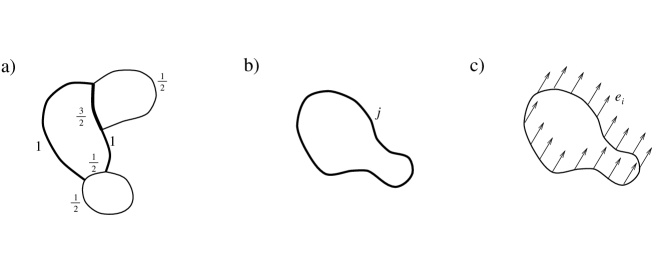
Figure 1: Panel a) illustrates a graph basis state. Graph basis bras, $\langle\Gamma|$, are linear combinations of loop basis bras that span the space of solutions to the Mandelstam constraints. That is, the graph amplitudes $\Psi[\Gamma]$ are independent and completely parametrize $SU(2)$ gauge invariant states $|\Psi\rangle$.

Panel b) shows a graph, $\gamma_{(j)}$, consisting of a single loop carrying spin $j$. When $j=\frac{1}{2}$ $\langle\gamma_{(j)}|$ is just the loop basis bra of the same loop. This loop basis bra can be represented by $tr\,H^{(\frac{1}{2})}[A,\gamma]$, the trace of the spin $\frac{1}{2}$ holonomy around $\gamma$, with the amplitude for the loop in a state $|\Psi\rangle$ given by the loop transform

$\ \ \ \Psi[\gamma]=\langle\gamma|\Psi\rangle=\int d\mu[A]\>(tr\,H^{(\frac{1}{2})}[A,\gamma])^{*}\>\Psi[A]$.

($\int d\mu[A]$ is an integral over $SU(2)$ connections defined on the relevant class of functionals of these connections). $\langle\gamma_{(j)}|$ is then represented by $tr\,H^{(j)}[A,\gamma]$. In other words, $\langle\gamma_{(j)}|$ for $j>\frac{1}{2}$ is just like the loop basis bra $\langle\gamma_{(\frac{1}{2})}|$ except the spin $j$ holonomy replaces the spin $\frac{1}{2}$ holonomy in the loop transform. When $d\mu[A]$ is taken to be the “induced Haar measure” (see [AL94]) graph basis states are orthonormal in the inner product $\langle\theta|\varphi\rangle=\int d\mu[A]\>\theta^{*}\varphi$, so we can think of $\Psi[\Gamma]$ as the coefficients in an expansion of the state $|\Psi\rangle$ on graph ket states $|\Gamma\rangle$, with $\langle A|\gamma_{(j)}\rangle=tr\,H^{(j)}[A,\gamma]$.

Panel c) shows an $\tilde{E}$ flux loop. In the classical limit $\hbar\rightarrow 0$, $j\sim O(1/\hbar)$ $\ |\gamma_{(j)}\rangle$ represents such a flux loop.

A particularly simple class of graphs are loops $\gamma$, without intersections, carrying spin $j$. In the classical limit the corresponding basis states $|\gamma,j\rangle$ represent isolated Faraday lines, or ‘flux loops’:

$$\tilde{E}^{a}_{i}=\pm e_{i}\int_{\gamma}\delta^{3}(x-z)dz^{a},$$ (6)

where $e_{i}$ has magnitude $j\hbar$ and is covariantly constant along $\gamma$. (See Appendix A for a proof and caveats).

Notice that on $\gamma$ $\ rank\tilde{E}=1$, and off $\gamma$ $\ \tilde{E}=0$, so we expect the evolution of these field configurations in the new canonical theory to differ from that in Ashtekar’s theory. Indeed in Ashtekar’s theory (6) can only evolve by 3-diffeomorphisms, i.e. they can move around in space, while in the new theory loops of $\tilde{E}$ flux can appear from, and disappear into ‘vacuum’, $\tilde{E}=0$. Appearances and disappearances of $\tilde{E}$ flux loops will be referred to, respectively, as ‘births’ and ‘deaths’.

The lack of births and deaths in the classical Ashtekar theory seems to be mirrored in it’s graph quantization. It was, in fact, the puzzling lack of births and deaths in a class of (formal) solutions to Ashtekar’s constraints found by Rovelli and Smolin in [RS88] that initially motivated me to rederive the constraints. In these solutions (called the RS solutions from here on) the graph representation of the state, $\Psi[\Gamma]$, is the characteristic function of the graph class (= equivalence class of graphs under 3-diffeos connected to the identity) of a graph, $\gamma$, consisting of one or more intersection free loops carrying spin $\frac{1}{2}$. In other words, if $K_{\gamma,\frac{1}{2}}$ is the graph class in question, the wave function is of the form

$$\Psi_{K_{\gamma,\frac{1}{2}}}[\Gamma]=\left\{\begin{array}[]{ll}1&\mbox{if $\Gamma\in K_{\gamma,\frac{1}{2}}$}\\ 0&\mbox{otherwise}\end{array}\right.$$ (7)

In such a state the number of loops is fixed, so there is zero amplitude for births and deaths of loops. Note that Rovelli and Smolin’s argument to the effect that $\Psi_{K_{\gamma,\frac{1}{2}}}$ solves the quantized constraints goes through unchanged if the loops are allowed to carry arbitrary spin, $j$.

Now suppose that a quantum theory of gravity possesses the spin $j$ RS solutions. Taking the $\hbar\rightarrow 0,\ \ j\sim O(1/\hbar)$ limit shows that $\tilde{E}$ flux loops can only evolve by 3-diffeos. No births or deaths are allowed in the classical theory. The theory is thus certainly not the Plebanski theory. In fact it will be argued in section 2 that the theory is not even fully 4-diffeo invariant.

It seems, therefore, that the new constraint (3) leads to births and deaths in the graph representation.

I should emphasize again, however, that, though motivated by quantum considerations, this paper deals exclusively with classical theory.

The remainder of this paper is organized as follows:

In section 2 the invariance of Ashtekar’s theory under all infinitesimal 4-diffeos , and its non-invariance under some finite 4-diffeos is established. Furthermore, it is argued that Ashtekar’s theory is not a gauge fixed version of any 4-diffeo invariant local theory, because it does not posses a ‘2-sphere solution’, which describes an $\tilde{E}$ flux loop being born from the vacuum, $\tilde{E}=0$, and eventually disappearing again.

In section 3 Plebanski’s action is derived from the familiar Hilbert-Palatini action and the field equations in Plebanski’s variables are found.

In section 4 a canonical formulation of Plebanski’s version of GR in terms of Ashtekar’s variables, $A$ and $\tilde{E}$, is derived from Plebanski’s action. (2) and (3) are the constraints of this formulation.

In section 5 a more elegant, but equivalent, canonical theory, in which the field $\phi^{ij}$ in (3) (which is, in fact, the left-handed Weyl curvature) and a conjugate momentum, $\tilde{\pi}_{ij}$, are treated as canonical coordinates.

Section 6 develops a ‘2-sphere solution’ to Plebanski’s spacetime field equations. In this solution both the self-dual curvature, $F^{i}_{\mu\nu}$, and the orthonormal basis of self-dual 2-forms, $\Sigma_{i\,\mu\nu}$, have support on a (thickened) 2-sphere in spacetime.

In section 7 it is shown that this 2-sphere solution solves the canonical theory of section 4. How the new Hamiltonian of section 4 generates the birth in this solution is explained in detail.

2 4-diffeomorphisms in Ashtekar’s canonical theory

Let’s begin by very briefly summarizing Ashtekar’s canonical theory in our notation. No proofs will be given since they can be found in e.g. [Ash91], and most statements will in fact be special cases of results of Section 4.

The canonical coordinates are the fields $A^{i}_{a}$ and $\tilde{E}^{a}_{i}$, which live on 3-space $\Sigma$ and have Poisson bracket

$$\{A^{i}_{a}(x),\tilde{E}^{b}_{j}(y)\}=\delta^{i}_{j}\delta^{b}_{a}\delta^{3}(x,y).$$ (8)

The constraints are

$$\tilde{\cal G}_{i} = D_{a}\tilde{E}^{a}_{i}=0$$ (9)

$$\tilde{\cal V}_{a} = \frac{1}{2}\epsilon_{abc}\tilde{B}^{i\,b}\tilde{E}^{a}_{i}=0$$ (10)

$$\>\tilde{\!\!\tilde{\cal S}} = \frac{1}{4}\epsilon_{abc}\tilde{B}^{i\,a}\tilde{E}^{b}_{j}\tilde{E}^{c}_{k}\epsilon_{i}{}^{jk}=0,$$ (11)

and the Hamiltonian is a sum of these constraints:

$$H_{Ash} = -\int_{\Sigma}\Lambda^{i}\tilde{\cal G}_{i}+N^{a}\tilde{\cal V}_{a}+\makebox[0.0pt][l]{\raisebox{-8.53581pt}[8.53581pt][-5.69054pt]{$\ \tilde{}$}}N\>\tilde{\!\!\tilde{\cal S}}\ d^{3}x$$ (12)

$$= -\int_{\Sigma}(\Lambda^{i}-N^{a}A^{i}_{a})\tilde{\cal G}_{i}+N^{a}\tilde{\Delta}_{a}+\makebox[0.0pt][l]{\raisebox{-8.53581pt}[8.53581pt][-5.69054pt]{$\ \tilde{}$}}N\>\tilde{\!\!\tilde{\cal S}}\ d^{3}x$$ (13)

$$= -G_{[\Lambda-N^{a}A_{a}]}-\Delta_{\vec{N}}-S_{\makebox[0.0pt][l]{\raisebox{-8.53581pt}[8.53581pt][-5.69054pt]{$\ \tilde{}$}}N},$$ (14)

where $\tilde{\Delta}_{a}=\tilde{\cal V}_{a}+A_{a}^{i}\tilde{\cal G}_{i}$, and $G_{\Lambda}=\int_{\Sigma}\Lambda^{i}\tilde{\cal G}_{i}\ d^{3}x$, $\Delta_{\vec{N}}=\int_{\Sigma}N^{a}\tilde{\Delta}_{a}\ d^{3}x$, and $S_{\makebox[0.0pt][l]{\raisebox{-8.53581pt}[8.53581pt][-5.69054pt]{$\ \tilde{}$}}N}=\int_{\Sigma}\makebox[0.0pt][l]{\raisebox{-8.53581pt}[8.53581pt][-5.69054pt]{$\ \tilde{}$}}N\>\tilde{\!\!\tilde{\cal S}}\ d^{3}x$.

This particular decomposition of the Hamiltonian into integrated constraints has the advantage that $G_{\Lambda}$ and $\Delta_{\vec{N}}$ have simple interpretations: $G_{\Lambda}$ generates $SO(3)_{0}$ gauge transformations, $\Delta_{\vec{N}}$ generates 3-diffeomorphisms. The constraint algebra is

$$\begin{array}[]{lll}\!\!\{G_{\Lambda_{1}},G_{\Lambda_{2}}\}=-G_{[\Lambda_{1},\Lambda_{2}]}&&\\ &&\\ \!\!\{G_{\Lambda},\Delta_{\vec{N}}\}=G_{\pounds_{\vec{N}}\Lambda}&\!\!\!\!\{\Delta_{\vec{N}_{1}},\Delta_{\vec{N}_{2}}\}=-\Delta_{[\vec{N}_{1},\vec{N}_{2}]}&\\ &&\\ \!\!\{G_{\Lambda},S_{\makebox[0.0pt][l]{\raisebox{-8.53581pt}[8.53581pt][-5.69054pt]{$\ \tilde{}$}}N}\}=0&\!\!\!\!\{\Delta_{\vec{N}},S_{\makebox[0.0pt][l]{\raisebox{-8.53581pt}[8.53581pt][-5.69054pt]{$\ \tilde{}$}}N}\}=-S_{\pounds_{\vec{N}}\makebox[0.0pt][l]{\raisebox{-8.53581pt}[8.53581pt][-5.69054pt]{$\ \tilde{}$}}N}&\!\!\!\!\{S_{\makebox[0.0pt][l]{\raisebox{-8.53581pt}[8.53581pt][-5.69054pt]{$\ \tilde{}$}}N_{1}},S_{\makebox[0.0pt][l]{\raisebox{-8.53581pt}[8.53581pt][-5.69054pt]{$\ \tilde{}$}}N_{2}}\}=\Delta_{\vec{K}}-G_{K^{a}A_{a}},\end{array}$$ (15)

with $K^{a}=K^{a}(\makebox[0.0pt][l]{\raisebox{-8.53581pt}[8.53581pt][-5.69054pt]{$\ \tilde{}$}}N_{1},\makebox[0.0pt][l]{\raisebox{-8.53581pt}[8.53581pt][-5.69054pt]{$\ \tilde{}$}}N_{2})=\tilde{E}^{i\,a}\tilde{E}^{a}_{i}\>(\makebox[0.0pt][l]{\raisebox{-8.53581pt}[8.53581pt][-5.69054pt]{$\ \tilde{}$}}N_{1}\partial_{b}\makebox[0.0pt][l]{\raisebox{-8.53581pt}[8.53581pt][-5.69054pt]{$\ \tilde{}$}}N_{2}-\makebox[0.0pt][l]{\raisebox{-8.53581pt}[8.53581pt][-5.69054pt]{$\ \tilde{}$}}N_{2}\partial_{b}\makebox[0.0pt][l]{\raisebox{-8.53581pt}[8.53581pt][-5.69054pt]{$\ \tilde{}$}}N_{1})$, $[\Lambda_{1},\Lambda_{2}]^{i}=\Lambda_{1}^{j}\Lambda_{2}^{k}\epsilon^{i}{}_{jk}$, and $[\vec{N}_{1},\vec{N}_{2}]^{a}=N_{1}^{b}\partial_{b}N_{2}^{a}-N_{2}^{b}\partial_{b}N_{1}^{a}$.

That completes the summary of Ashtekar’s theory. Now to diffeomorphisms.

Because the constraints (9), (10) and (11) are first class and complete, all gauge transformations of the classical state $(A,\tilde{E})$ are generated by $G_{\Lambda}$, $\Delta_{\vec{N}}$ and $S_{\makebox[0.0pt][l]{\raisebox{-8.53581pt}[8.53581pt][-5.69054pt]{$\ \tilde{}$}}N}$. Can a subset of these gauge transformations be interpreted as the group, $\mbox{\em Diff}_{0}(M)$, of 4-diffeos of spacetime, $M$, connected to the identity?

The history of $X\equiv(A,\tilde{E},\Lambda,\vec{N},\makebox[0.0pt][l]{\raisebox{-8.53581pt}[8.53581pt][-5.69054pt]{$\ \tilde{}$}}N)$ generated by the Hamiltonian can be thought of as a field configuration on the spacetime $M=\{({\cal P},t)|{\cal P}\in\Sigma,t\in{\bf R}\}$, in which the fields are described in terms of quantities that refer (like vector components refer to a basis) to the ‘slicing’ $\{\Sigma_{t}\}$, consisting of the equal $t$ 3-surfaces, and the ‘threading’ ${\gamma_{\cal P}}$, consisting of the constant ${\cal P}\in\Sigma$ worldlines.

Suppose another slicing and threading $\{\Sigma^{\prime}_{t^{\prime}}\}$, $\{\gamma^{\prime}_{{\cal P}^{\prime}}\}$ is defined by acting on the $\Sigma_{t}$ and $\gamma_{\cal P}$ with a 4-diffeo. What shall we take to be the corresponding fields $X^{\prime}=(A^{\prime},\tilde{E}^{\prime},\Lambda^{\prime},\vec{N}^{\prime},\makebox[0.0pt][l]{\raisebox{-8.53581pt}[8.53581pt][-5.69054pt]{$\ \tilde{}$}}N^{\prime})$? The quantities $X$ can, of course, be written as functions of the new ‘coordinates’ $({\cal P}^{\prime},t^{\prime})$, but they still refer to the old slicing and threading, and the $X$ need not a priori transform as scalars. The only a priori restriction on the (1 to 1) map $X\rightarrow X^{\prime}$ that will be made here is that it be local: $X^{\prime}$ at a spacetime point $p$ depends only on $X$ and the 4-diffeo within an infinitesimal neighborhood of $p$. (If we think of the 4-diffeos as active instead of passive then $X^{\prime}$ should depend only on $X$ and the diffeo near the pre-image of $p$).

The question is now: can this ‘local’ representation of diffeomorphisms carried by the fields $X$ be chosen so that each is a gauge transformation. In other words, can one define the map $X\rightarrow X^{\prime}$ in such a way that the history $X^{\prime}({\cal P}^{\prime},t^{\prime})$ is a gauge transform of the history $X({\cal P},t)$.

It turns out that the transformation of the canonical coordinates $(A,\tilde{E})$ generated by

$$J_{\xi}=\int_{\Sigma}\xi^{0}\tilde{\cal H}-\xi^{a}\tilde{\Delta}_{a}d^{3}x$$ (16)

can be interpreted as a 4-diffeo by the infinitesimal vector field $\xi^{\mu}$. ($\tilde{\cal H}=-(\Lambda^{i}-N^{a}A^{i}_{a})\tilde{\cal G}_{i}-N^{a}\tilde{\Delta}_{a}-\makebox[0.0pt][l]{\raisebox{-8.53581pt}[8.53581pt][-5.69054pt]{$\ \tilde{}$}}N\>\tilde{\!\!\tilde{\cal S}}$ is Ashtekar’s Hamiltonian density). One can see at once that $J_{\xi}$ generates the correct transformation in two simple cases. When $\xi^{0}$ is constant in 3-space and $\xi^{a}=0$ $J_{\xi}$ generates a time reparametrization $t\rightarrow t-\xi^{0}$. When $\xi^{0}=0$ $J_{\xi}$ generates 3-diffeos by $\vec{\xi}$.

The Lagrange multipliers are also transformed in a gauge transformation. A gauge transformed history is, after all, a history generated from the same initial data, but with altered Lagrange multipliers put into the Hamiltonian. The transformation law of the Lagrange multipliers can be derived from the requirement that the gauge transformed Hamiltonian generates the gauge transformed history of the canonical coordinates. Mathematically this requires

$$\delta^{o}_{\xi}H=\frac{\partial^{o}}{\partial t}J_{\xi}+\{J_{\xi},H\},$$ (17)

where the ^o means that the canonical coordinates are held fixed and only the Lagrange multipliers vary.

A rather intricate, but conceptually straightforward, calculation yields

$$\delta_{\xi}\makebox[0.0pt][l]{\raisebox{-8.53581pt}[8.53581pt][-5.69054pt]{$\ \tilde{}$}}N = \partial_{0}[\xi^{0}\makebox[0.0pt][l]{\raisebox{-8.53581pt}[8.53581pt][-5.69054pt]{$\ \tilde{}$}}N]+\pounds_{\vec{\xi}}\makebox[0.0pt][l]{\raisebox{-8.53581pt}[8.53581pt][-5.69054pt]{$\ \tilde{}$}}N-2\makebox[0.0pt][l]{\raisebox{-8.53581pt}[8.53581pt][-5.69054pt]{$\ \tilde{}$}}NN^{a}\partial_{a}\xi^{0}$$ (18)

$$\delta_{\xi}N^{a} = \partial_{0}[\xi^{0}N^{a}+\xi^{a}]+\pounds_{\vec{\xi}}N^{a}-N^{a}N^{b}\partial_{b}\xi^{0}-K^{a}(\xi^{0}\makebox[0.0pt][l]{\raisebox{-8.53581pt}[8.53581pt][-5.69054pt]{$\ \tilde{}$}}N,\makebox[0.0pt][l]{\raisebox{-8.53581pt}[8.53581pt][-5.69054pt]{$\ \tilde{}$}}N)$$ (19)

$$\delta_{\xi}\Lambda^{i} = [\pounds_{\xi}A]^{i}_{0},$$ (20)

where I have defined $A^{i}_{0}=\Lambda^{i}$, $\pounds_{\vec{\xi}}$ and $\pounds_{\xi}$ are the three and four dimensional Lie derivatives respectively, and $K^{a}(\makebox[0.0pt][l]{\raisebox{-8.53581pt}[8.53581pt][-5.69054pt]{$\ \tilde{}$}}N_{1},\makebox[0.0pt][l]{\raisebox{-8.53581pt}[8.53581pt][-5.69054pt]{$\ \tilde{}$}}N_{2})$ is defined as in the constraint algebra.

With these transformations, and

$$\delta_{\xi}A^{i}_{a}=\{A^{i}_{a},J_{\xi}\}\ \ \ \ \delta_{\xi}\tilde{E}^{a}_{i}=\{\tilde{E}^{i}_{a},J_{\xi}\}$$ (21)

the objects

$$A^{i}_{\mu}=\left[\begin{array}[]{c}\Lambda^{i}\\ A^{i}_{a}\end{array}\right]$$ (22)

and $\Sigma_{i\,\mu\nu}$, with

$$\Sigma_{i\,ab} = \frac{1}{2}\epsilon_{abc}\tilde{E}^{c}_{i}$$ (23)

$$\Sigma_{i\,0a} = \frac{1}{4}\makebox[0.0pt][l]{\raisebox{-8.53581pt}[8.53581pt][-5.69054pt]{$\ \tilde{}$}}N\epsilon_{abc}\epsilon_{i}{}^{jk}\tilde{E}^{b}_{j}\tilde{E}^{c}_{k}+\frac{1}{2}\epsilon_{abc}\tilde{E}^{b}_{i}N^{c},$$ (24)

transform as spacetime tensor fields when $A$ and $\tilde{E}$ are solutions to the evolution equations. That is

$$\delta_{\xi}A^{i}_{\mu} = \pounds_{\xi}A^{i}_{\mu}$$ (25)

$$\delta_{\xi}\Sigma_{i\,\mu\nu} = \pounds_{\xi}\Sigma_{i\,\mu\nu}.$$ (26)

Again the calculation is conceptually straightforward but quite tedious.

When $rank\ \tilde{E}\geq 2$ $A^{i}_{a}$, $\tilde{E}^{a}_{i}$, $\Lambda^{i}$, $N^{a}$, and $\makebox[0.0pt][l]{\raisebox{-8.53581pt}[8.53581pt][-5.69054pt]{$\ \tilde{}$}}N$ at a spacetime point $p$ are functions of $A^{i}_{\mu}$ and $\Sigma_{i\,\mu\nu}$ at $p$, so the transformation of these fields generated by $\delta_{\xi}$ is also a ‘local’ representation of the corresponding diffeomorphism. When $rank\ \tilde{E}<2$ $\makebox[0.0pt][l]{\raisebox{-8.53581pt}[8.53581pt][-5.69054pt]{$\ \tilde{}$}}N$, and possibly $N^{a}$, are undetermined by $A^{i}$ and $\Sigma_{i}$. However, the transformation of these fields, as determined by (18) and (19), is still a local representation of the diffeo. Ashtekar’s theory is, therefore, invariant under infinitesimal 4-diffeos.

Note also that $G_{\Lambda}$ and $J_{\xi}$ span the algebra of gauge generators (= first class constraints).

What about finite 4-diffeos? On certain solutions with degenerate $\tilde{E}$ the representation $\delta_{\xi}$ of the 4-diffeo generators cannot be integrated to give the whole proper 4-diffeo group $\mbox{\em Diff}_{0}(M)$ (Because $\makebox[0.0pt][l]{\raisebox{-8.53581pt}[8.53581pt][-5.69054pt]{$\ \tilde{}$}}N$ and $N^{a}$ blow up when some generators are iterated, see footnote 10).

This is most easily seen in solutions in which $\tilde{E}^{a}_{i}$ is a single unknotted flux loop and $A^{i}_{a}=0$. Then

$$\tilde{E}^{a}_{i}=e_{i}\int_{\gamma}\delta^{3}(x,z)dz^{a},$$ (31)

where $e_{i}$ is constant and $\gamma$ is diffeomorphic to a circle. In the gauge $\Lambda^{i}=0$ the evolution of the fields is given by

$$\dot{\tilde{E}}^{a}_{i} = \{\tilde{E}^{a}_{i},H_{Ash}\}=\pounds_{\vec{N}}\tilde{E}^{a}_{i}$$ (32)

$$\dot{A}^{i}_{a} = 0$$ (33)

so $\tilde{E}^{a}_{i}$ simply evolves by 3-diffeos.

In spacetime this solution is described by

$$\Sigma_{i\,\mu\nu} = \frac{1}{2}e_{i}\epsilon_{\mu\nu\rho\sigma}\int_{C}\delta^{4}(x-z)dz^{[\rho}dz^{\sigma]}$$ (34)

$$A^{i}_{\mu} = 0.$$ (35)

$C$ is the worldsheet of $\gamma$. Since $\gamma$ evolves only by 3-diffeos $C$ is topologically a 2-cylinder. Clearly there are 4-diffeos of $\Sigma_{i\,\mu\nu}$, and thus of $C$ (or, equivalently, of the slicing and threading) such that in the image the intersection $C\cap\Sigma_{t}$ is not a single loop for all $t$, but sometimes consists of several loops. (See Fig. 2). In other words, there are 4-diffeos of the history of $(A,\tilde{E})$ in which births and deaths of flux loops occur. This is, of course, not allowed by the evolution equations (32) and (33), so these 4-diffeo equivalent histories are not solutions. Ashtekar’s theory is thus not fully 4-diffeo invariant.

Figure 2: Two 4-diffeo equivalent evolutions of a flux loop. The cross sections of the 2-surfaces indicated by the dark lines are the flux loops at different times.

Could Ashtekar’s theory be seen as a partly gauge fixed formulation of a 4-diffeo invariant theory? Let’s, for the sake of argument, suppose that it is, then the solutions of the invariant theory would consist of all 4-diffeos of the solutions to Ashtekar’s theory. If the invariant theory is local, in the sense that it imposes only local field equations on the fields, then if a field configuration solves these equations in a basis of open sets it is a solution.

This is sufficient to show that the invariant theory has a ‘2-sphere’ solution in which $\Sigma_{i}$ is supported on a 2-sphere $S$ in spacetime:

$$\Sigma_{i\,\mu\nu} = \frac{1}{2}e_{i}\epsilon_{\mu\nu\rho\sigma}\int_{S}\delta^{4}(x-z)dz^{[\rho}dz^{\sigma]}$$ (36)

$$A^{i}_{\mu} = 0,$$ (37)

with $e_{i}$ constant. Within a sufficiently small open set one can always pick a slicing and threading so $\tilde{E}$ is a flux line evolving by 3-diffeos only (and $A=0$, $\Lambda=0$). The canonical evolution equations (32) and (33), and constraints (9),(10), and (11) thus hold within this open set, implying that the spacetime field equations also do.

The 2-sphere solution has births and deaths in any slicing, so it is not the diffeomorphic image of any solution of Ashtekar’s theory. Ashtekar’s theory is thus not a gauge fixed version of a local 4-diffeo invariant theory, because the gauge (slicing) in which there are no births and deaths does not exist for some solutions of any local theory having among its solutions all 4-diffeos of the solutions to Ashtekar’s theory.

Of course, the truncation of the 4-diffeomorphism symmetry we have seen in Ashtekar’s theory also occurs in standard Lorentzian canonical GR, because of the requirement that the $\Sigma_{t}$ be spacelike Cauchy surfaces. This condition also excludes some solutions of GR (solutions with closed timelike curves) from the canonical theory. This is sometimes even seen as an advantage of the canonical theory over the fully 4-diffeo invariant version because it ensures causality.

Here we have not imposed the Lorentzian reality conditions. If all the fields are taken to be real a Euclidean theory is obtained. Nevertheless an extension of the notion of causality to degenerate Euclidean geometries , such as the requirement that there be no births or deaths of flux loops, might justify the non-invariance of Ashtekar’s theory. Such a causality requirement is not entirely unreasonable since births and deaths are in fact ‘uncaused’ (gauge) - they cannot be predicted form the canonical initial data. Whether such causality conditions should be applied, especially in the quantum theory, is another question. The issue of causality in degenerate geometries needs to be explored further.

3 The Plebanski action

The Plebanski action will be used to define GR in this paper. In particular, the canonical theory of Section 4 is derived from it. It is classically equivalent to the Einstein-Hilbert (EH) action except in that, because it is well defined on a larger class of ‘geometries’ than the EH action, the space of classical solutions it defines is larger than that of the EH action. Not all extrema of the Plebanski action correspond to invertible metrics $g_{\mu\nu}$.

In this section the definition of the Plebanski action, and its relation to the EH action are reviewed (chiefly following [CDJ91] and [Ash91]), and the field equations defined by the Plebanski action are given.

Let’s begin by reviewing the concept of self-duality, taking the opportunity to fix notation along the way. In this paper we are concerned with (complex) Euclidean GR. The internal symmetry group is thus $SO(4)$, that is, gauge transformations of the vierbein $e_{I}{}^{\mu}$ preserve the internal metric $\delta_{IJ}$. ($SO(4)$ indices, which range over $\{0,1,2,3\}$, are represented by upper case latin letters from the middle of the alphabet: $I$, $J$, $K$, … . Spacetime indices are represented by lower case Greek letters.)

$SO(4)_{0}$ is the direct product of two factors of $SO(3)_{0}$, which will be called $SO(3)_{L}$ and $SO(3)_{R}$: $SO(4)_{0}=SO(3)_{L}\otimes SO(3)_{R}$. As a result $SO(4)$ tensors in the adjoint representation, and thus $SO(4)$ connections and curvatures, can be split into “self-dual” and “anti-self-dual” components, which transform under $SO(3)_{L}$ and $SO(3)_{R}$ respectively. Let’s see how this comes about.

The $SO(4)$ dual of an antisymmetric tensor $a^{IJ}$ is defined as

$$a^{\star\,IJ}=\frac{1}{2}\epsilon^{IJ}{}_{KL}a^{KL}.$$ (38)

$SO(4)_{0}$ transformations leave the duality operator $\frac{1}{2}\epsilon^{IJ}{}_{KL}=\frac{1}{2}\epsilon^{IJMN}\delta_{MK}\delta_{NL}$ invariant. Thus the adjoint representation, which acts on antisymmetric tensors $a^{[IJ]}$, reduces to a sum of representations acting in the two eigensubspaces of the duality operator, namely the self-dual representation acting on self-dual tensors $a^{+}=a^{+\star}$, and an anti-self-dual rep. acting on anti-self-dual tensors $a^{-}=-a^{-\star}$. Note that any antisymmetric tensor $a^{IJ}$ can be split into a self-dual and an anti-self-dual component according to

$$a^{\pm}=\frac{1}{2}[a\pm a^{\star}].$$ (39)

(Anti-)self-dual tensors have only three independent components. According to their definition $a^{\pm ij}=\pm\epsilon^{ij}{}_{k}a^{\pm 0k}\$ ($i,j,k\in\{1,2,3\}$) so we may take the independent components to be

$$a^{\pm i}=\pm 2a^{\pm 0i}.$$ (40)

The $so(4)$ generators are themselves adjoint rep. tensors. Decomposing these into their self-dual and anti-self-dual components lets us rewrite the $so(4)$ commutation relations

$$[G_{IJ},G_{KL}]=-\{\delta_{I[K}G_{L]J}-\delta_{J[K}G_{L]I}\}$$ (41)

as

$$[G^{+}_{i},G^{+}_{j}] = \epsilon_{ij}{}^{k}G^{+}_{k}$$ (42)

$${[}G^{+}_{i},G^{-}_{j}] = 0$$ (43)

$${[}G^{-}_{i},G^{-}_{j}] = \epsilon_{ij}{}^{k}G^{-}_{k},$$ (44)

which defines two commuting $so(3)$ algebras. In other words $SO(4)_{0}=SO(3)_{L}\otimes SO(3)_{R}$ where, in the adjoint rep. of $SO(4)$ $SO(3)_{L}$ acts on self-dual tensors, and $SO(3)_{R}$ acts on anti-self-dual tensors. Specifically, $a^{+i}$ and $a^{-i}$ transform as, respectively, $SO(3)_{L}$ and $SO(3)_{R}$ vectors. generators, $SO(3)_{L}$ From here on $SO(3)$ indices, which run over $\{1,2,3\}$, will always be represented by lower case latin letters, $i$,$j$,$k$,…, from the middle of the alphabet. Note that upper and lower $SO(3)$ indices are equivalent since the $SO(3)$ metric is $\delta_{ij}$.

It is a remarkable fact that an action can be written for GR involving only self-dual, or left-handed, quantities, so that the internal symmetry group becomes simply $SO(3)$. The Plebanski action is such an action. It is

$$I=\int\frac{1}{2}\Sigma_{i}\wedge F^{i}-\frac{1}{4}\phi^{ij}\Sigma_{i}\wedge\Sigma_{j}.$$ (45)

$F^{i}_{\mu\nu}=2\partial_{[\mu}A^{i}_{\nu]}+\epsilon^{i}{}_{jk}A^{j}_{\mu}A^{k}_{\nu}$ is the curvature of the $SO(3)$ connection $A^{i}_{\mu}$. $\Sigma_{i\,\mu\nu}$ is an $SO(3)$ vector 2-form, and $\phi^{ij}$, which is required to be trace free ($\phi^{ij}\delta_{ij}=0$) acts as a Lagrange multiplier.

The field equations implied by the stationary of $I$ under variations of $\phi$, $A$ and $\Sigma$ are, respectively

$$\Sigma_{i}\wedge\Sigma_{j} \propto \delta_{ij}\epsilon$$ (46)

$$D\wedge\Sigma_{i} = 0$$ (47)

$$F^{i}-\phi^{ij}\Sigma_{j} = 0.$$ (48)

Here $\epsilon_{\kappa\lambda\mu\nu}$ is the spacetime antisymmetric symbol, which can be thought of as the coordinate volume form. On tensors with only $SO(3)$ indices $D$ is the covariant derivative with connection $A$. For example, $D_{\mu}v^{i}=\partial_{\mu}v^{i}+A^{j}_{\mu}\epsilon^{i}{}_{jk}v^{k}$ ($\epsilon^{i}{}_{jk}$ is the $j$th generator of $SO(3)$ in the fundamental rep.). $D_{[\mu}\Sigma_{\nu\lambda]}$ in (47) is evaluated using a torsionless extension of $D$ to spacetime tensors. Which torsionless extension is used is immaterial because of the antisymmetrization of the spacetime indices.

In appendix B it is shown that if $v=\frac{2}{3}\Sigma_{i}\wedge\Sigma^{i}\neq 0$ then (46) implies that there exists a non-singular tetrad $e^{I}{}_{\mu}$, unique up to $SO(3)_{R}<SO(4)$ transformations on the internal index $I$, such that

$$\Sigma_{i}=\frac{1}{2}e^{0}\wedge e^{i}+\frac{1}{4}\epsilon_{ijk}e^{j}\wedge e^{k}.$$ (49)

In other words, $\Sigma_{i}$ is the self dual part of $\frac{1}{2}e^{I}\wedge e^{J}$ with respect to the internal 4-metric $\delta_{IJ}$. Note that $e^{I}{}_{\mu}$ forms an orthonormal tetrad with respect to the spacetime metric $g_{\mu\nu}=e^{I}{}_{\mu}e^{J}{}_{\nu}\delta_{IJ}$, and that $v=e^{0}\wedge e^{1}\wedge e^{2}\wedge e^{3}$ is the volume form of this metric.

In the following it will be shown that if $v\neq 0$ in an open region, $U$, then the field equations (47) and (48) imply that the metric $g_{\mu\nu}=e^{I}{}_{\mu}e^{J}{}_{\nu}\delta_{IJ}$ solves Einstein’s vacuum field equation, $R_{\mu\nu}[g]=0$, in $U$, and $A^{i}_{\mu}$ is the self-dual part of the metric compatible $SO(4)$ connection $\omega_{\mu}^{IJ}=e_{\alpha}{}^{J}[\partial_{\mu}e^{\alpha I}+\{{}^{\,\alpha}_{\beta\mu}\}e^{\beta I}]$. ($\{{}^{\,\alpha}_{\beta\mu}\}$ is the spacetime connection of $g$).

Conversely, taking as $(\Sigma_{i},A^{i})$ the self-dual parts of $(\frac{1}{2}e^{I}\wedge e^{J},\ \omega^{IJ})$ in a solution to Einstein’s field equation on $U$ yields a solution to (46), (47) and (48) (with suitably chosen $\phi$) in which $v\neq 0$ in $U$. The set of solutions to (46), (47) and (48) with $v\neq 0$ is thus just the set of solutions to Einstein’s vacuum equation.

There are also solutions to (46), (47) and (48) with $v=0$. These do not correspond to solutions of Einstein’s equations in good coordinates, since the geometrical volume of finite coordinate volumes is zero, and some do not correspond to any coordinatization of a solution to Einstein’s equations. Such solutions will be the focus of this paper.

Now let’s prove the equivalence of the $v\neq 0$ sector of Plebanski’s theory with standard GR. We begin by restricting the Plebanski action to solutions of (46). The $\Sigma_{i}$ are then parametrized by $e^{I}{}_{\mu}$ according to (49). Specifically, $\Sigma_{i}$ is the self-dual part of $\frac{1}{2}e^{I}\wedge e^{J}$ with respect to the internal metric $\delta_{IJ}$. Thus on solutions of (46)

$$I=\frac{1}{2}\int\Sigma_{i}\wedge F^{i}=\frac{1}{4}\int e_{I}\wedge e_{J}\wedge F^{IJ},$$ (51)

where $F^{IJ}$, defined by $F^{0i}=\frac{1}{2}F^{i}$, $F^{ij}=\frac{1}{2}\epsilon^{ij}{}_{k}F^{k}$, is the curvature of the self-dual connection $A^{IJ}$, defined similarly by $A^{0i}=\frac{1}{2}A^{i}$, $A^{ij}=\frac{1}{2}\epsilon^{ij}{}_{k}A^{k}$.

Because $F^{IJ}$ is self-dual

$$I=\frac{1}{8}\int e^{I}\wedge e^{J}\wedge F^{KL}\epsilon_{IJKL} = \frac{1}{8}\int\epsilon^{\kappa\lambda\mu\nu}e^{I}{}_{\kappa}e^{J}{}_{\lambda}F^{KL}_{\mu\nu}\epsilon_{IJKL}\ d^{4}x$$ (52)

$$= \frac{1}{2}\int e\ e_{K}{}^{\mu}e_{L}{}^{\nu}F^{KL}_{\mu\nu}\ d^{4}x,$$ (53)

where $e=det[e^{I}{}_{\mu}]$. (53) is the self-dual action for GR found by Samuel [Sam87] and Jacobson and Smolin [JS87], [JS88].

Let $\nabla$ be the (unique) torsionless derivative compatible with the spacetime metric $g_{\mu\nu}=e^{I}{}_{\mu}e^{J}{}_{\nu}\delta_{IJ}$, and extend its action to internal indices by requiring $\nabla e^{I}{}_{\mu}=0$. The internal connection coefficients of $\nabla$ are then $\omega_{\mu}^{IJ}=e_{\alpha}{}^{J}[\partial_{\mu}e^{\alpha I}+\{{}^{\,\alpha}_{\beta\mu}\}e^{\beta I}]$. Define $C^{+}$ as the difference between the self-dual connection $A^{IJ}$ and the self-dual part $\omega^{+IJ}$ of the metric connection: $C^{+IJ}_{\mu}=A^{IJ}_{\mu}-\omega^{+IJ}_{\mu}$. $F$ can then be expanded as a sum of the curvature, $R^{+}$, of $\omega^{+}$, and terms in $C^{+}$:

$$F^{IJ}_{\mu\nu}=R^{+IJ}_{\mu\nu}+2\nabla_{[\mu}C^{+IJ}_{\nu]}+2C^{+IM}_{[\mu}C^{+}_{\nu]M}{}^{J}$$ (54)

$R^{+}$ is the self-dual part of the Riemann curvature tensor. Thus, from (53),

$$I=\frac{1}{2}\int e\ e_{K}{}^{\mu}e_{L}{}^{\nu}\ \{R^{+KL}_{\mu\nu}+2\nabla_{\mu}C^{+KL}_{\nu}+2C^{+KM}_{[\mu}C^{+}_{\nu]M}{}^{L}\}\ d^{4}x.$$ (55)

Consider the first term in (55).

$$e\ e^{\mu}_{K}e^{\nu}_{L}\ R^{+KL}_{\mu\nu} = \frac{1}{2}\,e\ [e^{\mu}_{K}e^{\nu}_{L}R^{KL}_{\mu\nu}+\frac{1}{2}e^{\mu}_{K}e^{\nu}_{L}\epsilon^{KL}{}_{IJ}R^{IJ}_{\mu\nu}]$$ (56)

$$= \frac{1}{2}\sqrt{g}[R+\frac{1}{2}\epsilon^{\kappa\lambda\mu\nu}R_{\kappa\lambda\mu\nu}]=\frac{1}{2}\sqrt{g}R,$$ (57)

since $R^{\kappa}{}_{[\lambda\mu\nu]}=0$. The first term in (55) is thus just the Einstein-Hilbert action $I_{EH}=\frac{1}{4}\int R\sqrt{g}d^{4}x$. The second term in the integrand of (55) is a divergence, since $\nabla e_{I}{}^{\mu}=0$. $I$ is thus a sum of the Einstein-Hilbert action, a surface term, and a potential term quadratic in the field $C^{+}$ which does not enter the Einstein-Hilbert action.

$$I=I_{EH}+\mbox{\em surface term}+\int e\ e^{\mu}_{[K}e^{\nu}_{L]}\,C^{+KM}_{\mu}C^{+}_{n\,M}{}^{L}\ d^{4}x.$$ (58)

By splitting $C^{+}$ into judiciously chosen components the $C^{+}$ potential term can be diagonalized. Define $C^{+JK}_{I}=e_{I}{}^{\mu}C^{+JK}_{\mu}$, then let $C^{+K}=C^{+IK}_{I}$ and $\bar{C}^{+IJK}=C^{+IJK}-\frac{2}{3}\delta^{I[J}C^{+K]}-C^{+[IJK]}$ (so that $\delta_{IJ}\bar{C}^{+IJK}=0$ and $\bar{C}^{+[IJK]}=0$). The three tensors, $C^{+K}$, $C^{+[IJK]}$, and $\bar{C}^{+IJK}$ are independent components of $C^{+IJK}$, with no constraints correlating them. In terms of these components the $C^{+}$ potential term is

$$V=\int e\ \{-\frac{1}{3}C^{+M}C^{+}_{M}+\frac{1}{4}\bar{C}^{+KLM}\bar{C}^{+}{}_{KLM}-\frac{1}{2}C^{+[KLM]}C^{+}{}_{[KLM]}\}\ d^{4}x$$ (59)

This potential clearly has no zero modes, so extremizing $I$ with respect to $C^{+}$ (equivalently, solving (47), $\frac{\delta I}{\delta A}=0$) requires $C^{+}=0$, in other words, $A=\omega^{+}$. Furthermore, on the extremum with respect to $C^{+}$, $I$ is equivalent to $I_{EH}$. That is to say, the only remaining field equation, (48), $\frac{\delta I}{\delta\Sigma}=0$, becomes $0=\frac{\delta I}{\delta g_{\mu\nu}}=\frac{\delta I_{EH}}{\delta g_{\mu\nu}}$. As is well known, $\frac{\delta I_{EH}}{\delta g_{\mu\nu}}=0\Leftrightarrow R_{\mu\nu}+\frac{1}{2}Rg_{\mu\nu}=0\Leftrightarrow R_{\mu\nu}=0$, which is just the Einstein vacuum field equation. This proves that solutions of (46), (47), and (48) with $v=\frac{2}{3}\Sigma_{i}\wedge\Sigma^{i}\neq 0$ correspond to solutions of Einstein’s equation. The converse is clear.

4 Canonical formulation in terms of Ashtekar’s variables

To derive the canonical theory corresponding to the Plebanski action we begin by choosing a slicing of spacetime $M$ into 3-surfaces $\Sigma_{t}$, parametrized by ‘time’ $t\in{\bf R}$, and all diffeomorphic to one another (and thus to $\Sigma=\Sigma_{0}$). The $\Sigma_{t}$ will not be assumed to be ‘spacelike’, i.e. to have a positive definite, and thus non-degenerate, spatial metric, since in many of the degenerate solutions we are interested in this condition is not met by any slicing. Since this paper is not concerned with the effects of a non-trivial topology of $\Sigma$ or $M$ these are assumed, for simplicity and definiteness, to be diffeomorphic to $S^{3}$ and $S^{3}\times{\bf R}$ respectively. The canonical variables will be fields living on $\Sigma$.

In addition to the slicing we also need to choose a ‘threading’, a congruence of curves, $\{\gamma_{\cal P}|{\cal P}\in\Sigma\}$, transverse to the $\Sigma_{t}$ and filling spacetime, which mark the world lines of ‘the same point’ in 3-space $\Sigma$. The solutions to the canonical theory will correspond to the evolution, in $t$, of the fields on the slices $\Sigma_{t}$ in a solution to the spacetime field equations, with the time derivative at a point ${\cal P}\in\Sigma$ in the canonical theory corresponding to $d/dt$ along $\gamma_{\cal P}$ in spacetime. $M$, $\Sigma$ and the slicing and threading are illustrated schematically in Fig. 3.

Figure 3: Schematic illustration of spacetime $M$ and space $\Sigma$, in which $M=S^{3}\times{\bf R}$ and $\Sigma=S^{3}$ are represented by $S^{1}\times{\bf R}$ and $S^{1}$ respectively. The slicing, $\{\Sigma_{t}|t\in{\bf R}\}$, and threading, $\{\gamma_{\cal P}|{\cal P}\in\Sigma\}$, of $M$ are indicated, as well as the ‘time flow’ vector field $v=\frac{d}{dt}|_{\gamma_{\cal P}}$.

The tangent vector field, $v=\frac{d}{dt}|_{\gamma_{\cal P}}$ of the $\gamma_{\cal P}$ is called the “time flow vector”. In the standard treatment of canonical GR the metric is used to decompose $v$ into a piece $N^{\mu}$ tangent to $\Sigma_{t}$ and a piece $Nn^{\mu}$ normal to $\Sigma_{t}$, where $n$ is the unit future pointing normal to $\Sigma_{t}$. $N$ is called the lapse, and $N^{\mu}$ is called the shift. This decomposition is not always well defined in the degenerate solutions we are considering, so it will not be made here.

Once a slicing and a threading has been chosen $v$ and $dt$ can be used to make a $3+1$ decomposition of the tensor fields appearing in the action. That is, each such tensor is decomposed into spatial ($\Sigma_{t}$) tensor components. In local coordinates, $x^{\mu}$, adapted to the slicing and threading in that $x^{0}=t$ and $\frac{dx^{a}}{dt}|_{\gamma_{\cal P}}=0$, this boils down to writing the Lagrangian density as a sum of terms in which each spacetime index is replaced by $0$ or a spatial index. The Plebanski action (45) becomes

$$I=\int\epsilon^{0abc}\Sigma_{i\,bc}F^{i}_{0a}+\epsilon^{0abc}\Sigma_{i\,0a}F^{i}_{bc}-\phi^{ij}\epsilon^{0abc}\Sigma_{i\,0a}\Sigma_{j\,bc}\ d^{4}x.$$ (60)

Here $\epsilon$ is the antisymmetric symbol with $\epsilon^{0123}=1$.

(60) can be put in a nice form using the definitions $\epsilon^{abc}=\epsilon^{0abc}$, $\tilde{B}^{i\,a}=\epsilon^{abc}F^{i}_{bc}$ and

$$\tilde{E}^{a}_{i}=\epsilon^{abc}\Sigma_{i\,bc},$$ (61)

and the identity $F^{i}_{0a}=\partial_{0}A^{i}_{a}-D_{a}A^{i}_{0}$ (in which $A^{i}_{0}$ is differentiated as though it were an $SO(3)$ vector). After an integration by parts (60) becomes

$$I = \int\ \int_{\Sigma_{t}}\tilde{E}^{a}_{i}\,\partial_{0}A^{i}_{a}+A^{i}_{0}D_{a}\tilde{E}^{a}_{i}+\Sigma_{i\,0a}\tilde{B}^{i\,a}-\Sigma_{i\,0a}\phi^{ij}\tilde{E}^{a}_{j}\ d^{3}x\ dt$$ (62)

$$= \int\ \int_{\Sigma_{t}}\tilde{E}^{a}_{i}\partial_{0}A^{i}_{a}-\tilde{\cal H}\ d^{3}x\ dt.$$ (63)

Recall that $\Sigma_{t}$ is assumed closed, so there are no boundary terms.

Plebanski’s action can thus be seen as a phase space action for GR. One can read off that $\tilde{E}^{a}_{i}(x)$ is the momentum conjugate to $A^{i}_{a}(x)$, and that the Hamiltonian density is

$$\tilde{\cal H}=-A^{i}_{0}D_{a}\tilde{E}^{a}_{i}-\Sigma_{i\,0a}[\tilde{B}^{i\,a}-\phi^{ij}\tilde{E}^{a}_{j}].$$ (64)

$A^{i}_{0}$, $\Sigma_{i\,0a}$, and $\phi^{ij}$ enter (62) as Lagrange multipliers. The classical state, $(A,\tilde{E})$, must therefore satisfy the constraints

$$D_{a}\tilde{E}^{a}_{i} = 0$$ (2)

$$\exists\phi^{ij}\mbox{trace free, symmetric} \ni \tilde{B}^{i\,a}-\phi^{ij}\tilde{E}^{a}_{j}=0.$$ (3)

These constraints are the spatial parts of the field equations (47) and (48):

$$\begin{array}[]{rclcl}D\wedge\Sigma_{i}&=&0&\Rightarrow&0=D_{[a}\Sigma_{i\,bc]}=\frac{1}{3!}D_{d}\tilde{E}^{d}_{i}\epsilon_{abc}\\ F^{i}-\phi^{ij}\Sigma_{j}&=&0&\Rightarrow&0=F^{i}_{ab}-\phi^{ij}\Sigma_{j\,ab}=\frac{1}{2}\epsilon_{abc}[\tilde{B}^{i\,a}-\phi^{ij}\tilde{E}^{a}_{j}]\end{array}$$ (65)

The time components of these equations give the evolution of $A$ and $\tilde{E}$, in terms of $A^{i}_{0}$, $\Sigma_{i\,0a}$, and $\phi^{ij}$.

Stationarity of the action with respect to variations of $\phi^{ij}$ implies field equation (46)

$$\begin{array}[]{rclcl}\Sigma_{i}\wedge\Sigma_{j}&\propto&\delta_{ij}&\Leftrightarrow&\Sigma_{(i\,0a}\tilde{E}^{a}_{j)}\propto\delta_{ij},\end{array}$$ (66)

which places no constraint on the state, $(A,\tilde{E})$, since $\Sigma_{i\,0a}$ is a Lagrange multiplier and may thus be freely chosen. However, for a given state it constrains $\Sigma_{i\,0a}$, which restricts the possible evolutions of the state.

(2) and (3) are the primary constraints. In fact, they are the complete constraints, since they are preserved by the Hamiltonian evolution, without further conditions on the state. (However, the conditions (66), (111), and (112) on the Lagrange multiplier $\Sigma_{i\,0a}$, are necessary).

Before proving the completeness of the constraints (2) and (3), let’s pause to understand what we have found so far.

(3) is not of the usual form “constraint function = 0”. Rather, it demands merely that, for any admissible $(A,\tilde{E})$ there exists a traceless, symmetric $\phi^{ij}$ such that $\tilde{B}^{i\,a}-\phi^{ij}\tilde{E}^{a}_{j}$ vanishes.

The content of (3) becomes clearer when $\phi$ is eliminated. When $rank\tilde{E}=3$ ($\tilde{E}^{a}_{i}$ invertible)

$$\phi^{ij}=\tilde{B}^{i\,a}\makebox[0.0pt][l]{\raisebox{-8.53581pt}[8.53581pt][-5.69054pt]{$\ \tilde{}$}}E^{-1\,j}_{a}=\tilde{B}^{i\,a}\epsilon^{jkl}\epsilon_{abc}\tilde{E}^{b}_{k}\tilde{E}^{c}_{l}/2det\tilde{E}.$$ (67)

The constraints arise from the requirement that $\phi^{ij}$ be symmetric and trace free.

Symmetry requires

$$0 = \tilde{B}^{[i\,a}\epsilon^{j]kl}\epsilon_{abc}\tilde{E}^{b}_{k}\tilde{E}^{c}_{l}$$ (68)

$$= -\epsilon^{ijk}\epsilon_{abc}\tilde{B}^{l\,a}\tilde{E}^{b}_{l}\tilde{E}^{c}_{k},$$ (69)

which holds if and only if

$$\epsilon_{abc}\tilde{B}^{i\,a}\tilde{E}^{b}_{i}=0.$$ (70)

The tracelessness of $\phi^{ij}$ requires

$$0 = \delta_{ij}\ \tilde{B}^{i\,a}\epsilon^{jkl}\epsilon_{abc}\tilde{E}^{b}_{k}\tilde{E}^{c}_{l}$$ (71)

$$= \epsilon^{ijk}\epsilon_{abc}\tilde{B}^{i\,a}\tilde{E}^{b}_{j}\tilde{E}^{c}_{k}.$$ (72)

(70) and (72) (and (2)) are just Ashtekar’s constraints. As shown in [CDJM91], when $rank\tilde{E}=3$, the Plebanski action leads exactly to Ashtekar’s canonical theory. It is less obvious, but nevertheless true, that (3) is equivalent to Ashtekar’s constraints (70) and (72) also when $rank\tilde{E}=2$. This is shown in Appendix C.

When $rank\tilde{E}=1$. $\tilde{E}^{a}_{i}$ is of the form $e_{i}\tilde{w}^{a}$. (3) requires that $\tilde{B}^{i\,a}$ is also proportional to $\tilde{w}^{a}$: $\tilde{B}^{i\,a}=b^{i}\tilde{w}^{a}$, with $b^{i}-\phi^{ij}e_{k}=0$. A symmetric, traceless $\phi$ can always be found which satisfies this last condition. Thus, when $rank\tilde{E}=1$ (3) is equivalent to

$$\tilde{B}^{i[a}\tilde{E}^{b]}_{j}=0.$$ (73)

When $\tilde{E}^{a}_{i}=0$ (3) is equivalent to

$$\tilde{B}^{i\,a}=0.$$ (74)

Summarizing:

$$rank\tilde{E} 3 2 0=\epsilon_{abc}\tilde{B}^{i\,a}\tilde{E}^{b}_{i} 0=\epsilon^{ijk}\epsilon_{abc}\tilde{B}^{i\,a}\tilde{E}^{b}_{j}\tilde{E}^{c}_{k} 0=\epsilon_{abc}\tilde{B}^{i\,a}\tilde{E}^{b}_{j} 0=\tilde{B}^{i\,a}$$ (3) equivalent to or (70) (72) 1 (73) 0 (74) (75)

Note that both (73) and (74) imply (70) and (72), so (2) and (3) always imply Ashtekar’s constraints. However, when $rank\tilde{E}\leq 1$, the converse is not true. The solution set of (2) and (3) is the Ashtekar constraint surface with parts of the surface $rank\tilde{E}\leq 1$ cut out.

The solution set can be thought of as an infinite dimensional generalization of that shown in Fig. 4, which corresponds to the constraint $\exists\phi\in{\bf R}\ni q-\phi p=0$ on the classical state $(q,p)$ of a one degree of freedom system.

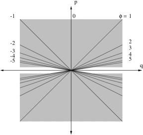
Figure 4: The solutions, $(q,p)$, to the constraint $\exists\phi\in{\bf R}\ni q-\phi p=0$ are shaded in grey. Note that the only excluded points are $p=0,\ q\in(-\infty,0)\cup(0,\infty)$. $\ (q,p)=(0,0)$ is not excluded by the constraint.

Clearly (3), even though it contains the Lagrange multiplier $\phi$, is more elegant than (75). Moreover, as shown in Section 3, $\phi$ is the left-handed Weyl curvature (in $SO(3)$ tensor notation), which in the null initial value formulation of Lorentzian GR of [PR84] contains the local degrees of freedom of the gravitational field. It therefore seems best to keep $\phi$ in the canonical theory. At the end of this section a slightly different canonical formulation will be given, in which $\phi$ is treated as a configuration variable. In that formulation the constrained phase space takes on a more conventional, manifold like, form.

Now we understand the constraint (3) a little better. What about (66)? And what is the significance of $\tilde{E}^{a}_{i}$ and $\Sigma_{i\,0a}$?

To give some idea of what $\tilde{E}^{a}_{i}$ and $\Sigma_{i\,0a}$ represent I will evaluate them in terms of tetrads on a slice, $\Sigma_{t}$, of a non-degenerate solution to the field equation (46), $\Sigma_{i}\wedge\Sigma_{j}\propto\delta_{ij}\epsilon$, (which is equivalent to (66)). It was shown in Appendix B that, when (46) holds and $\Sigma_{i}\wedge\Sigma^{i}\neq 0$, $\Sigma_{i}$ defines a non-degenerate, orthonormal co-tetrad $e_{\mu}^{I}$, unique up to $SO(3)_{R}$ transformations, so that

$$\Sigma_{i\,\mu\nu}=e^{0}_{[\mu}e^{i}_{\nu]}+\frac{1}{2}\epsilon_{ijk}e^{j}_{\mu}e^{k}_{\nu}.$$ (76)

Now the generators of $SO(3)_{R}$ are the anti-self-dual parts of the generators of $SO(4)$, so $SO(3)_{R}$ transformations consist of an $SO(4)$ boost by an arbitrary rapidity $\theta^{i}$, accompanied by a spatial rotation by an angle $|\theta|$ about $\theta^{i}$. Hence $e^{0}_{\mu}$ can be brought to any unit vector, provided the rest of the tetrad is rotated appropriately. We will take $e^{0}_{\mu}=n_{\mu}$, the future pointing unit normal to $\Sigma_{t}$. Then $e^{0}_{a}=0$. Denoting the spatial co-triad $e^{i}_{a}$, in the adapted gauge, by $E^{i}_{a}$ we find

$$\Sigma_{i\,ab} = \frac{1}{2}\epsilon_{ijk}E^{j}_{a}E^{k}_{b}$$ (77)

$$= \frac{1}{2}\epsilon_{abc}E^{c}_{i}\ det[E^{i}_{a}],$$ (78)

where $E^{a}_{i}$ is the inverse of $E^{i}_{a}$. Applying the definition (61) one finds $\tilde{E}^{a}_{i}=E^{a}_{i}\ det[E^{i}_{a}]$, showing that $\tilde{E}^{a}_{i}$ is the densitized spatial triad.

Using this same gauge we can calculate $\Sigma_{i\,0a}$ in terms of $\tilde{E}^{a}_{i}$ and the lapse, $N$, and shift, $N^{a}$, defined by the time flow vector $v$ via

$$v^{\mu}=Nn^{\mu}+N^{\mu},\ \ \ N^{\mu}n_{\mu}=0.$$ (79)

Since $e^{0}_{0}=n_{\mu}v^{\mu}=N$ and $e^{i}_{0}=e^{i}_{\mu}v^{\mu}=e^{i}_{\mu}N^{\mu}=E^{i}_{a}N^{a},$

$$\Sigma_{i\,0a} = \frac{1}{2}N\,E^{i}_{a}+\frac{1}{2}\epsilon_{ijk}\,E^{j}_{c}E^{k}_{a}N^{c}$$ (80)

$$= \frac{1}{4}\makebox[0.0pt][l]{\raisebox{-8.53581pt}[8.53581pt][-5.69054pt]{$\ \tilde{}$}}N\epsilon_{i}{}^{jk}\epsilon_{abc}\,\tilde{E}^{b}_{j}\tilde{E}^{c}_{k}+\frac{1}{2}\epsilon_{abc}\tilde{E}^{b}_{i}N^{c}.$$ (81)

Here $\makebox[0.0pt][l]{\raisebox{-8.53581pt}[8.53581pt][-5.69054pt]{$\ \tilde{}$}}N=N/det[E^{i}_{a}].$

(81) can also be derived within the canonical theory from (66), and the assumption that $\tilde{E}^{a}_{i}$ is non-singular. (66), $\Sigma_{(i\,0a}\tilde{E}^{a}_{j)}\propto\delta_{ij}$, implies

$$\Sigma_{i\,0a}\tilde{E}^{a}_{j}=\tilde{c}_{1}\delta_{ij}+\tilde{c}_{2}^{k}\epsilon_{ikj},$$ (82)

where $\tilde{c}_{1}$ and $\tilde{c}_{2}^{k}$ are arbitrary densities. If $rank\tilde{E}=3$ then (81) follows immediately from (82) by contracting it with the inverse of $\tilde{E}$, $\makebox[0.0pt][l]{\raisebox{-8.53581pt}[8.53581pt][-5.69054pt]{$\ \tilde{}$}}E_{a}^{-1\,i}=\frac{1}{2}\epsilon^{ijk}\epsilon_{abc}\tilde{E}^{b}_{j}\tilde{E}^{c}_{k}/det\tilde{E}$, and setting $\makebox[0.0pt][l]{\raisebox{-8.53581pt}[8.53581pt][-5.69054pt]{$\ \tilde{}$}}N=2\tilde{c}_{1}/det\tilde{E}$, and $N^{c}=2\tilde{c}^{k}_{2}\tilde{E}^{c}_{k}/det\tilde{E}$.

Solutions to (66) are still of the form (81) where $rank\tilde{E}=2$ (see Appendix C). However, where $rank\tilde{E}\leq 1$ (81) is not the complete solution. Rather, the general solution is

$$\Sigma_{i\,0a}=\frac{1}{2}\epsilon_{abc}\tilde{E}^{b}_{j}N^{j\,c}_{i},$$ (83)

which has two more degrees of freedom. Finally, when $\tilde{E}^{a}_{i}=0$ $\Sigma_{i\,0a}$ is completely unconstrained by (66).

In [CDJM91] Capovilla, Dell, Jacobson and Mason derive Ashtekar’s theory from the Plebanski action by solving (66) (assuming $rank\tilde{E}=3$) for $\Sigma_{i\,0a}$, obtaining the lapse-shift form (81), then substituting this form into the $3+1$ action (62). Extremization of the action with respect to $N^{c}$ and $\makebox[0.0pt][l]{\raisebox{-8.53581pt}[8.53581pt][-5.69054pt]{$\ \tilde{}$}}N$ then yielded Ashtekar’s constraints (70) and (72) respectively. As the reader may easily verify, the constraints (75) can be derived in the same way if the form of $\Sigma_{i\,0a}$ appropriate to the rank of $\tilde{E}$ is inserted into the action (62).

The derivation of [CDJM91] leads to Ashtekar’s Hamiltonian (12),

$$H_{Ash}=-G_{A_{0}}-\int_{\Sigma}s_{i\,a}(\makebox[0.0pt][l]{\raisebox{-8.53581pt}[8.53581pt][-5.69054pt]{$\ \tilde{}$}}N,\vec{N},\tilde{E})\tilde{B}^{i\,a}\ d^{3}x,$$ (84)

where $s_{i\,a}$ is the lapse-shift form of $\Sigma_{i\,0a}$, instead of the integral of (64),

$$H_{\Sigma}=-G_{A_{0}}-\int_{\Sigma}\Sigma_{i\,0a}[\tilde{B}^{i\,a}-\phi^{ij}\tilde{E}^{a}_{j}]\ d^{3}x.$$ (85)

In fact, when $\Sigma_{i\,0a}=s_{i\,a}$, the two are equivalent. Clearly $\{\tilde{E}^{a}_{i},H_{\Sigma}\}=\frac{\delta H_{\Sigma}}{\delta{A_{a}^{i}}}|_{\Sigma_{i\,0a}=s_{i\,a}}=\{\tilde{E}^{a}_{i},H_{Ash}\}$. Less obviously

$$\{A^{i}_{a},H_{Ash}+G_{A_{0}}\}=-\frac{\delta s_{j\,b}}{\delta\tilde{E}^{a}_{i}}\tilde{B}^{j\,b}=-\frac{\delta s_{j\,b}}{\delta\tilde{E}^{a}_{i}}\phi^{jk}\tilde{E}^{b}_{k}=0+s_{j\,a}\phi^{ji}=\{A^{i}_{a},H_{\Sigma}+G_{A_{0}}\}$$ (86)

by (3) and (66).

We now turn to proving the completeness of the constraints (2) and (3). To establish completeness we must show that the constraints (2) and (3) are preserved in the evolution, generated by the Hamiltonian, of any initial $(A,\tilde{E})$ satisfying (2) and (3).

Note that, since (3) requires only that there exists $\phi^{ij}$, symmetric and traceless, such that $\tilde{B}^{i\,a}-\phi^{ij}\tilde{E}^{a}_{j}=0$, (3) is preserved by the evolution of the state $(A,\tilde{E})$ provided there is a corresponding evolution of $\phi$ such that $\tilde{B}^{i\,a}-\phi^{ij}\tilde{E}^{a}_{j}$ remains zero. In other words (3) is preserved if

$$0=\frac{d}{dt}[\tilde{B}^{i\,a}-\phi^{ij}\tilde{E}^{a}_{j}]=\{\tilde{B}^{i\,a}-\phi^{ij}\tilde{E}^{a}_{j}\,,H\}-\frac{d\phi^{ij}}{dt}\tilde{E}^{a}_{j}$$ (87)

can be solved by some $\frac{d\phi^{ij}}{dt}$.

The Hamiltonian is a sum of two parts proportional to the ‘constraint functions’ appearing in (2) and (3): $H=H_{1}+H_{2}$, with $H_{1}=-G_{A_{0}}=-\int_{\Sigma}A^{i}_{0}D_{a}\tilde{E}^{a}_{i}d^{3}x$ and $H_{2}=\int_{\Sigma}\Sigma_{i\,0a}[\tilde{B}^{i\,a}-\phi^{ij}\tilde{E}^{a}_{j}]d^{3}x$.

The Gauss law constraint (2), and thus $H_{1}$, generates $SO(3)$ gauge transformations. For infinitesimal $\Lambda^{i}$

$$\delta_{\Lambda}A^{i}_{a}(x) = \{A_{a}^{i}(x),\int_{\Sigma}\Lambda^{j}D_{b}\tilde{E}^{b}_{j}d^{3}y\}=-D_{a}\Lambda^{i}(x)$$ (88)

$$\delta_{\Lambda}\tilde{E}_{i}^{a}(x) = \{\tilde{E}_{i}^{a}(x),\int_{\Sigma}\Lambda^{j}D_{b}\tilde{E}^{b}_{j}d^{3}y\}$$ (89)

$$= \{\tilde{E}_{i}^{a}(x),-\int_{\Sigma}\Lambda^{j}\epsilon_{jk}{}^{l}A_{b}^{k}\tilde{E}^{b}_{l}d^{3}y\}$$ (90)

$$= -\Lambda^{j}\epsilon_{ij}{}^{k}\tilde{E}^{a}_{k}(x)$$ (91)

is an infinitesimal $SO(3)$ gauge transformation.

The gauss law constraint (2) transforms homogeneously under $SO(3)$ gauge transformations of $A$ and $\tilde{E}$, so it is preserved by the evolution generated by $H_{1}$. That it is also preserved by $H_{2}$ can be seen as follows

$$\{G_{\Lambda},H_{2}\} = \{G_{\Lambda},-\int_{\Sigma}\Sigma_{j\,0b}[\tilde{B}^{j\,b}-\phi^{jk}\tilde{E}^{b}_{k}]d^{3}y\}$$ (92)

$$= \int_{\Sigma}\Sigma_{i\,0a}[\delta_{\Lambda}\tilde{B}^{i\,a}-\phi^{ij}\delta_{\Lambda}\tilde{E}^{a}_{j}]d^{3}x$$ (94)

$$= -\int_{\Sigma}\delta_{\Lambda}\Sigma_{i\,0a}[\tilde{B}^{i\,a}-\phi^{ij}\tilde{E}^{a}_{j}]d^{3}x$$

$$\int_{\Sigma}\delta_{\Lambda}\phi^{ij}\Sigma_{(i\,0a}\tilde{E}^{a}_{j)}d^{3}x$$

$$\approx 0,$$ (95)

where $\delta_{\Lambda}$ now denotes the extension to all fields of the $SO(3)$ gauge transformation generated by $G_{\Lambda}$, and $\approx 0$ means that the quantity vanishes on states solving the constraints. The first term in (95) vanishes when (3) holds, while the second vanishes by virtue of the restriction (66) on $\Sigma_{i\,0a}$.

To check whether (3) is preserved we first compute $\{\tilde{B}^{i\,a}-\phi^{ij}\tilde{E}^{a}_{j},H\}$.

$$\{\tilde{B}^{i\,a}-\phi^{ij}\tilde{E}^{a}_{j},H_{1}\}\approx-\delta_{A_{0}}\phi^{ij}\tilde{E}^{a}_{j}=-2A_{0}^{k}\epsilon^{(i}{}_{kl}\phi^{j)l}\tilde{E}^{a}_{j}.$$ (96)

Now, for arbitrary $w^{1}_{i\,a}$ and $w^{2}_{i\,a}$

$$\{\int_{\Sigma}w^{1}_{i\,a}[\tilde{B}^{i\,a}-\phi^{ij}\tilde{E}^{a}_{j}]\ d^{3}x_{1},\int_{\Sigma}w^{2}_{k\,b}[\tilde{B}^{k\,b}-\phi^{kl}\tilde{E}^{b}_{l}]\ d^{3}x_{2}\}$$ (97)

$$= \{\int_{\Sigma}w^{1}_{i\,a}\tilde{B}^{i\,a}\ d^{3}x_{1},-\int_{\Sigma}w^{2}_{k\,b}\phi^{kl}\tilde{E}^{b}_{l}\ d^{3}x_{2}\}\ -\ 1\leftrightarrow 2$$ (98)

$$= -2\int_{\Sigma}[D_{a}w^{1}_{i\,b}]w^{2}_{j\,c}\epsilon^{abc}\phi^{ij}d^{3}x\ -\ 1\leftrightarrow 2$$ (99)

$$= 2\int_{\Sigma}w^{1}_{i\,a}w^{2}_{j\,b}D_{c}\phi^{ij}\epsilon^{abc}\ d^{3}x,$$ (100)

so

$$\{\tilde{B}^{i\,a}-\phi^{ij}\tilde{E}^{a}_{j},H_{2}\}=-2\Sigma_{j\,0b}D_{c}\phi^{ij}\epsilon^{abc}$$ (101)

(Note that the extremization of the action (62) with respect to $\Sigma_{i\,0a}$ requires the $\phi$ appearing in $H$ to be a $\phi$ which renders $\tilde{B}^{i\,a}-\phi^{ij}\tilde{E}^{a}_{j}$ zero).

(87) thus requires that

$$0 = \dot{\phi}^{ij}\tilde{E}^{a}_{j}+2A_{0}^{k}\epsilon^{(i}{}_{kl}\phi^{j)l}\tilde{E}^{a}_{j}-2D_{b}\phi^{ij}\Sigma_{j\,0c}\epsilon^{abc}$$ (106)

$$= D_{0}\phi^{ij}\tilde{E}^{a}_{j}-2D_{b}\phi^{ij}\Sigma_{j\,0c}\epsilon^{abc}.$$ (107)

When $\Sigma_{i\,0a}$ is of the lapse-shift form (81) (107) can always be solved by some $D_{0}\phi^{ij}$. When $\Sigma_{i\,0a}$ is of this form

$$\Sigma_{j\,0c}\epsilon^{abc}=\frac{1}{2}\makebox[0.0pt][l]{\raisebox{-8.53581pt}[8.53581pt][-5.69054pt]{$\ \tilde{}$}}N\epsilon_{j}{}^{kl}\tilde{E}^{a}_{k}\tilde{E}^{b}_{l}+\tilde{E}^{[a}_{j}N^{b]}.$$ (108)

Hence (107) becomes

$$0=[D_{0}\phi^{ij}-N^{b}D_{b}\phi^{ij}-\makebox[0.0pt][l]{\raisebox{-8.53581pt}[8.53581pt][-5.69054pt]{$\ \tilde{}$}}N\epsilon_{k}{}^{jl}\tilde{E}^{b}_{l}D_{b}\phi^{ik}]\tilde{E}^{a}_{j}+D_{b}\phi^{ij}\tilde{E}^{b}_{j}N^{a}.$$ (109)

The last term vanishes when (2) and (3) hold, while the term in brackets vanishes for suitable $D_{0}\phi^{ij}$, so the equation can be solved.

When $rank\tilde{E}\geq 2$ (66) requires $\Sigma_{i\,0a}$ to be of the lapse-shift form. Hence (107) doesn’t imply any new restrictions on the Lagrange multipliers at a given time. In general the solvability of (107) requires that

$$\exists\theta^{ij}\mbox{trace free, symmetric}\ni 2D_{b}\phi^{ij}\Sigma_{j\,0c}\epsilon^{abc}=\theta^{ij}\tilde{E}^{a}_{j}.$$ (110)

(If this is true $D_{0}\phi^{ij}=\theta^{ij}$ solves (107)). (110) is of the same form as (3). Its content can be extracted by eliminating $\theta$. One finds

$$0=\tilde{E}^{[d}_{k}\epsilon^{a]bc}D_{b}\phi^{ij}\Sigma_{j0c}\ \ \mbox{if $rank\tilde{E}=1$,}$$ (111)

and,

$$0=\epsilon^{abc}D_{b}\phi^{ij}\Sigma_{j0c}\ \ \mbox{if $\tilde{E}=0$}.$$ (112)

(The contraction on $k$ and $i$ of the right side of (111) vanishes by (2), (3), and (66), but the trace free part produces new restrictions on $\Sigma_{i\,0a}$).

For any $A$, $\tilde{E}$, and $\phi$ the restrictions (111) and (112) are solved by $\Sigma_{i\,0a}$ of the lapse shift form, as well as many others. Thus the preservation in time of (3) does not require further, secondary constraints on $(A,\tilde{E})$, nor, in fact, on $\phi$.

5 Canonical formulation treating the Weyl curvature as a configuration variable

An illuminating alternative canonical formulation of the Plebanski theory elevates $\phi^{ij}$ to the status of a configuration variable. This is actually a very natural thing to do. As pointed out in Section 3, $\phi^{ij}$ is really just the left-handed Weyl curvature (in $SO(3)$ tensor language). In the null initial value formulation of Lorentzian GR of [PR84] a certain (complex) component of $\phi^{ij}$ constitutes the local degrees of freedom of the gravitational field on the null initial surface.

$\phi^{ij}$ will thus be given a momentum $\tilde{\pi}_{ij}$ which will be constrained to be zero. To keep the gauge invariance of the theory manifest, the momentum $\tilde{\pi}$ will be ‘created’ by adding a gauge invariant term to the Plebanski action. The new action is

$$I^{\prime}=\int\frac{1}{2}\Sigma_{i}\wedge F^{i}-\frac{1}{4}\phi^{ij}\Sigma_{i}\wedge\Sigma_{j}+\Pi_{ij}\wedge D\phi^{ij}+\Pi_{ij}\wedge K^{ij}.$$ (113)

The 3-form $\Pi_{ij}$ is symmetric and traceless in $ij$, and the 1-form $K^{ij}$ is a Lagrange multiplier which enforces $\Pi_{ij}=0$. Note that the content of the theory is completely unchanged, only the formalism describing it is being modified.

A $3+1$ decomposition, and the definitions $\tilde{\pi}_{ij}=-\epsilon^{abc}\Pi_{ij\,abc}$ and $\kappa^{ij}=K_{0}^{ij}$, yields

$$I^{\prime} = \int\int_{\Sigma_{t}}\tilde{E}^{a}_{i}\partial_{0}A^{i}_{a}+\tilde{\pi}_{ij}D_{0}\phi^{ij}+A_{0}^{i}D_{a}\tilde{E}^{a}_{i}+\Sigma_{i\,0a}[\tilde{B}^{i\,a}-\phi^{ij}\tilde{E}^{a}_{j}]$$ (115)

$$\ \ \ +\tilde{\pi}_{ij}\kappa^{ij}+3\epsilon^{abc}\Pi_{ij\,0ab}[D_{c}\phi^{ij}+K_{c}^{ij}]\ d^{3}x\ dt$$

Extremization with respect to $K_{c}^{ij}$ requires $\Pi_{ij\,0ab}=0$. We may substitute this equation into the action and simply drop the last term. Then we obtain a phase space action which shows that the fundamental Poisson brackets are

$$\{A^{i}_{a}(x),\tilde{E}^{b}_{j}(y)\} = \delta^{i}_{j}\delta^{a}_{b}\delta^{3}(x,y)$$ (116)

$$\{\phi^{ij}(x),\tilde{\pi}_{kl}(y)\} = [\delta^{(i}_{k}\delta^{j)}_{l}-\frac{1}{3}\delta^{ij}\delta_{kl}]\delta^{3}(x,y),$$ (117)

the primary constraints are

$$\tilde{\cal G}^{\prime}_{i} = D_{a}\tilde{E}^{a}_{i}+2\epsilon^{j}{}_{il}\phi^{lk}\tilde{\pi}_{jk}=0$$ (118)

$$\tilde{\cal C}^{i\,a} = \tilde{B}^{i\,a}-\phi^{ij}\tilde{E}^{a}_{j}=0$$ (119)

$$\tilde{\pi}_{ij} = 0$$ (120)

and the Hamiltonian is

$$H=-\int_{\Sigma}A^{i}_{0}\ \tilde{\cal G}^{\prime}_{i}+\Sigma_{i\,0a}\ \tilde{\cal C}^{i\,a}+\kappa^{ij}\ \tilde{\pi}_{ij}\ d^{3}x.$$ (121)

$G_{\Lambda}=\int_{\Sigma}\Lambda^{i}\tilde{\cal G}^{\prime}_{i}\ d^{3}x$ not only generates an $SO(3)$ gauge transformation of $A$ and $\tilde{E}$, as shown in (88) and (91), but also generates the corresponding gauge transformations of $\phi$ and $\tilde{\pi}$:

$$\{\phi^{ij},G_{\Lambda}\} = -2\Lambda^{k}\epsilon^{(i}{}_{kl}\phi^{j)l}=\delta_{\Lambda}\phi^{ij}$$ (122)

$$\{\tilde{\pi}_{ij},G_{\Lambda}\} = -2\Lambda^{k}\epsilon_{(ik}{}^{l}\tilde{\pi}_{j)l}=\delta_{\Lambda}\tilde{\pi}_{ij}.$$ (123)

The algebra of the integrated constraints $G_{\Lambda}$, $C_{w}=\int_{\Sigma}w_{i\,a}\tilde{\cal C}^{i\,a}\ d^{3}x$ and $P_{u}=\int_{\Sigma}u^{ij}\tilde{\pi}_{ij}\ d^{3}x$ now follows immediately from (117), (100) and the fact that $G_{\Lambda}$ generates the $SO(3)$ gauge transformations $\delta_{\Lambda}$:

$$\{G_{\Lambda_{1}},G_{\Lambda_{2}}\} = G_{[\Lambda_{1},\Lambda_{2}]}$$ (124)

$$\{G_{\Lambda},C_{w}\} = C_{\delta_{\Lambda}\,w}$$ (125)

$$\{G_{\Lambda},P_{u}\} = P_{\delta_{\Lambda}\,u}$$ (126)

$$\{C_{w^{1}},C_{w^{2}}\} = 2\int_{\Sigma}w^{1}_{i\,a}w^{2}_{j\,b}\>D_{c}\phi^{ij}\epsilon^{abc}\ d^{3}x$$ (127)

$$\{C_{w},P_{u}\} = -\int_{\Sigma}w_{(i\,a}\tilde{E}^{a}_{j)}\ u^{ij}\ d^{3}x$$ (128)

$$\{P_{u_{1}},P_{u_{2}}\} = 0$$ (129)

where $[\Lambda_{1},\Lambda_{2}]^{i}=\epsilon^{i}{}_{jk}\Lambda_{1}^{j}\Lambda_{2}^{k}$ and $u^{ij}$ is (without loss of generality) taken to be trace free. (127) and (128) show that some of these constraints are second class.

Nevertheless, when the restrictions on $\Sigma_{i\,0a}$ found in our previous $(A,\tilde{E})$ formulation of the canonical theory hold, the constraints are preserved by evolution, so they are complete:

$$\frac{d}{dt}G_{\Lambda} = \{G_{\Lambda},H\}+G_{\frac{d\Lambda}{dt}}$$ (130)

$$= H[\delta_{\Lambda}A^{i}_{0},\delta_{\Lambda}\Sigma_{i\,0a},\delta_{\Lambda}\kappa^{ij}]+G_{\frac{d\Lambda}{dt}}$$ (131)

$$\approx 0$$ (132)

$$\frac{d}{dt}\tilde{\cal C}^{i\,a} \approx \kappa^{ij}\tilde{E}^{a}_{j}-2D_{c}\phi^{ij}\Sigma_{j\,0b}\epsilon^{abc}$$ (133)

$$\frac{d}{dt}\tilde{\pi}_{ij} \approx -\Sigma_{(i\,0a}\tilde{E}^{a}_{j)}-\frac{1}{3}\delta_{ij}\mbox{\em trace}.$$ (134)

The constraints are preserved provided

$$\Sigma_{(i\,0a}\tilde{E}^{a}_{j)}\propto\delta_{ij}$$ (135)

$$\kappa^{ij}\tilde{E}^{a}_{j}-2D_{c}\phi^{ij}\Sigma_{j\,0b}\epsilon^{abc}=0.$$ (136)

(135) is of course just the familiar restriction (66). Noting that the evolution equation of $\phi$ can be written as $D_{0}\phi^{ij}=-\kappa^{ij}$ we see that (136) is just (107):

$$D_{0}\phi^{ij}\tilde{E}^{a}_{j}+D_{c}\phi^{ij}\Sigma_{j\,0b}\epsilon^{abc}=0.$$ (137)

(136) can thus be solved for $\kappa^{ij}$ if and only if $\Sigma_{i\,0a}$ satisfies the conditions (135), (111) and (112). If these conditions, which place no constraints on the classical state $(A,\tilde{E},\phi,\tilde{\pi})$, hold, then evolution preserves the primary constraints. Hence there are no secondary constraints.

Let’s consider the constraint surface of our second canonical formulation. An analogous system with two degrees of freedom $q$ and $\phi$, with conjugate momenta $p$ and $\pi$ respectively, is

$$q-\phi p = 0$$ (142)

$$\pi = 0.$$ (143)

The phase space is four dimensional but (143) shows that the constraint surface lies in the three dimensional subspace $\pi=0$, so it can be visualized. It is seen to be an infinite two dimensional plane which has been twisted, like a ribbon, by a $180^{\circ}$ rotation of the $\phi=+\infty$ end relative to the $\phi=-\infty$ end. (See Figure 5). Note that it is a manifold with no singularities.

Figure 5: A part of the constraint surface $q-\phi p=0$, $\pi=0$. The $\pi$ axis is not shown. The constraint manifold is a two dimensional ruled surface, composed of the lines $q-\phi p=0$ at every fixed $\phi$. These lines rotate by $180^{\circ}$ from $\phi=-\infty$ to $\phi=+\infty$.

Not surprisingly it is much harder to see what singularities the solution set of the constraints (118), (119) and (120) has. However this much can be said. Since this solution set is the intersection of the zeros of polynomials in the canonical variables it should not have any cuts (i.e. excluded lower dimensional submanifolds) because it should, in some sense, be a closed set.

The second class nature of the constraints poses a formidable obstacle to canonical quantization. A short attempt did not yield any simple expression for the Dirac bracket. The most promising approach, in the authors opinion, is to take advantage of the simplicity of (119) to eliminate $A$ in favor of the other canonical variables. This seems difficult at first, because $A$ cannot be expressed locally in terms of $\tilde{B}$ (and thus $\tilde{E}$ and $\phi$ via (119)).

However, by integration, (3) can be turned into an expression for the $SO(3)$ holonomies in terms of $\tilde{E}$ and $\phi$ given in a suitable gauge. Thus (3) might be solvable if the gravitational field is described in terms of holonomies (and some additional variables to completely coordinatize phase space).

One might try to work either with the non-canonical classical loop variables of Rovelli and Smolin [RS90], or with the canonical ‘Faraday line’ variables of Newman and Rovelli [NR92], which describe the ($SO(3)$ gauge equivalence classes of) classical states as configurations of $\tilde{E}$ flux lines, and fields canonically conjugate to those describing the flux lines.

The author hopes that ultimately solving (3) will lead to a description of the gravitational field in terms of loops and a dynamical $\phi$ field carrying the local degrees of freedom of the field. Be that as it may, the problem of eliminating (3) will not be discussed further in this paper.

6 Spacetime 2-sphere solution

A ‘2-sphere solution’ is a solution to the spacetime field equations in which the basis, $\Sigma_{i}$, of self-dual 2-forms, and the $SO(3)$ curvature, $F^{i}$, both have support on an (unknotted) 2-sphere in spacetime, or, as is the case in the present paper, on a thickened 2-sphere.

In Section 2 it was argued that Ashtekar’s canonical theory is not fully 4-diffeomorphism invariant because it does not have a 2-sphere solution, even though there is a 2-sphere spacetime field configuration which solves the canonical theory on a suitable slicing of a neighborhood of any point, and thus would be a solution if Ashtekar’s theory were fully 4-diffeo invariant. Here it will be shown that there is such a 2-sphere solution to the spacetime field equations of Plebanski’s theory (3). In Section 7 I will demonstrate that this spacetime field configuration, viewed as a field history, also solves the canonical formulation of Plebanski’s theory that was worked out in Section 4. 2-sphere solutions are especially interesting from the point of view of canonical theory because they involve the birth and death of loops of $\tilde{E}$ and $\tilde{B}$ flux. How, precisely, this comes about will be shown in Section 7.

We will begin with the ansatz

$$\Sigma_{i}=e_{i}\sigma\equiv e_{i}\int_{0}^{1}d\lambda_{1}\int_{0}^{1}d\lambda_{2}\ \Delta^{*}_{S_{\lambda}}(x)$$ (144)

and then derive a corresponding $A^{i}$ such that the field equations (46), (47) and (48) are solved. $e_{i}$ is an $SO(3)$ vector field which will ultimately determine the internal direction of the $\tilde{E}^{a}_{i}$ in the canonical treatment. Without loss of generality $e$ is taken to be non-zero. $\{S_{\lambda}\}$ is a family of 2-spheres parametrized by $\lambda_{A}\in\Box\equiv[0,1]^{2}$. The $S_{\lambda}$ do not intersect each other, nor do they ‘bunch up’ - the parameters $\lambda_{A}$ are required to be continuous functions on the part of spacetime occupied by the $S_{\lambda}$. $\Delta^{*}_{S_{\lambda}\>\mu\nu}=\frac{1}{2}\epsilon_{\mu\nu\sigma\rho}\Delta^{\sigma\rho}_{S_{\lambda}}$ is the spacetime dual of the characteristic distribution of $S_{\lambda}$: $\Delta_{S_{\lambda}}^{\mu\nu}(x)=\int_{S_{\lambda}}\delta^{4}(x-z)\>dz^{[\mu}dz^{\nu]}$. $\Delta_{S}^{\mu\nu}$ is a generalization to 2-surfaces of the current of a worldline. It can be thought of as a second degree delta function with support on $S$, times the local tangent bivector of $S$. More on characteristic distributions can be found in Appendix D.

In (144) $\Sigma_{i}$ is supported on a 2-sphere thickened in two dimensions, i.e. on a 4-volume ${\cal S}=\cup_{\lambda\in\Box}S_{\lambda}$. This has the advantage that the fields are regular enough that the theory of Sections 3 and 4 can be applied without modification.

Now let’s find the consequences of each of the field equations in turn within the ansatz (144).

(46) requires $\Sigma_{i}\wedge\Sigma_{j}\propto\delta_{ij}\epsilon$. According to (144)

$$\Sigma_{i}\wedge\Sigma_{j}=e_{i}e_{j}\sigma\wedge\sigma.$$ (147)

Note that the independent tangents to $S_{\lambda}$, $t_{1}$ and $t_{2}$, satisfy $t_{A}^{[\mu}\Delta_{S_{\lambda}}^{\nu]\sigma}=0$, which implies $t_{A}^{\mu}\Delta^{*}_{S_{\lambda}\>\mu\nu}=0$. Since $\lambda_{A}$ are continuous on ${\cal S}$ a unique $S_{\lambda}$ passes through each point of ${\cal S}$. Hence $t_{1}^{\mu}$ and $t_{2}^{\mu}$ are spacetime vector fields with the property $t_{A}^{\mu}\sigma_{\mu\nu}=0$ on ${\cal S}$, which is the support of $\sigma$. $\sigma\wedge\sigma=0$ follows immediately, and thus $\Sigma_{i}\wedge\Sigma_{j}=0$, implying that (46) holds identically in the ansatz (144).

(47) requires $D\wedge\Sigma_{i}=0$, or equivalently $D_{\mu}\Sigma^{*\>\mu\nu}_{i}=0$. According to (144)

$$D_{\mu}\Sigma^{*\>\mu\nu}_{i}=D_{\mu}e_{i}\sigma^{*\>\mu\nu}+e_{i}\partial_{\mu}\sigma^{*\>\mu\nu}.$$ (148)

$**=1$ and (261) then show that

$$\partial_{\mu}\sigma^{*\>\mu\nu}=\int_{\Box}d^{2}\lambda\ \partial_{\mu}\Delta^{\mu\nu}_{S_{\lambda}}=-\frac{1}{2}\int_{\Box}d^{2}\lambda\ \Delta^{\nu}_{\partial S_{\lambda}}.$$ (149)

Since the $S_{\lambda}$ are 2-spheres $\partial S_{\lambda}=\emptyset$ which means that the second term in (148) vanishes. (47) thus requires

$$D_{\mu}e_{i}\sigma^{*\,\mu\nu}=0.$$ (150)

But $\sigma^{*\,\mu\nu}\propto t_{1}^{[\mu}t_{2}^{\nu]}$ (the tangent bivector of the $S_{\lambda}$ passing through the point), so (150) implies that $t_{A}^{\mu}D_{\mu}e_{i}=0$, i.e. that $e$ is covariantly constant on the $S_{\lambda}$!

(48) requires $F^{i}-\phi^{ij}\Sigma_{j}=0$. (144) then implies that

$$F^{i}=\phi^{ij}e_{j}\sigma=b^{i}\sigma.$$ (151)

$F^{i}$ also has support on ${\cal S}$, and $t_{A}^{\mu}F^{i}_{\mu\nu}=0$. The connection is thus flat on each $S_{\lambda}$. Since the $S_{\lambda}$, being 2-spheres, have no non-contractable curves, the condition that $e$ be covariantly constant on $S_{\lambda}$ can be solved because parallel transport is completely path independent on $S_{\lambda}$.

Hence, to find a solution to all the field equations with $\Sigma_{i}$ of the form (144) one only needs to find a connection, $A^{i}$, having curvature $F^{i}=b^{i}\sigma$, with $b^{i}-\phi^{ij}e_{j}=0$ and $e_{i}$ covariantly constant on $S_{\lambda}$.

The Bianchi identity,

$$D\wedge F^{i}=0,$$ (152)

requires (in analogy to (47)) that $t_{a}^{\mu}D_{\mu}b^{i}=0$. $b$ must, like $e$, be covariantly constant on $S_{\lambda}$. $b$ is, however, not further constrained by the requirement $b^{i}-\phi^{ij}e_{j}=0$. For arbitrary $SO(3)$ vectors $b$ and $e$ ($e\neq 0$) this requirement is met by

$$\phi^{ij}=\frac{1}{e_{1}}\left[\begin{array}[]{ccc}b^{1}&b^{2}&b^{3}\\ b^{2}&\theta-b^{1}&\varphi\\ b^{3}&\varphi&-\theta\end{array}\right]$$ (153)

where the internal $1$ axis has been taken to lie along $e$. The degrees of freedom $\theta$ and $\varphi$ can be set arbitrarily at every point without affecting any other fields in the solution. They can, and will, be set to zero. Then $\phi$ too is covariantly constant on the $S_{\lambda}$.

Beyond the Bianchi identity the existence of an $A^{i}$ poses no further restrictions on $F^{i}=b^{i}\sigma$. $A^{i}$ is easily found in the gauge in which $e$ has constant components on each $S_{\lambda}$, i.e. $e_{i}=e_{i}(\lambda)$, and $b$ has constant components on all of ${\cal S}$. Since the $S_{\lambda}$ are closed there exist 3-manifolds $U_{\lambda}$ such that $\partial U_{\lambda}=S_{\lambda}$ Moreover, the $U_{\lambda}$ may be chosen so that they do not cut any $S_{\lambda}$ transversely. That is to say, if $S_{\lambda}$ touches $U_{\lambda^{\prime}}$ then it lies entirely in $U_{\lambda^{\prime}}$. Now let

$$A^{i}=b^{i}\alpha\equiv 3!b^{i}\int_{\Box}d^{2}\lambda\ \Delta^{*}_{U_{\lambda}},$$ (154)

and set the components of $b$ constant on all spacetime. Then

$$F^{i}=d\wedge A^{i}+\epsilon^{i}{}_{jk}A^{j}\wedge A^{k}=b^{i}d\wedge\alpha+\alpha\wedge\alpha\>b^{j}b^{k}\epsilon^{i}{}_{jk}=b^{i}d\wedge\alpha.$$ (155)

From (261) of Appendix D

$$d\wedge\alpha=3!\int_{\Box}d^{2}\lambda\ d\wedge\Delta^{*}_{U_{\lambda}}=\int_{\Box}d^{2}\lambda\ \Delta^{*}_{S_{\lambda}}=\sigma,$$ (156)

so indeed $F^{i}=b^{i}\sigma$.

The $U_{\lambda}$ have been chosen so that the tangents, $t_{A}^{\mu}$, to the $S_{\lambda}$ are also tangent to $U_{\lambda}$. It follows that $t_{A}^{\mu}A_{\mu}^{i}=0$, i.e. the connection components along $S_{\lambda}$ vanish, which shows that $e_{i}=e_{i}(\lambda)$ and $b^{i}$ are covariantly constant on the $S_{\lambda}$. We have found the solution corresponding to ansatz (144)!

This solution can be stated, in the same gauge, with less emphasis on the 2-surfaces $S_{\lambda}$:

$$A^{i}_{\mu} = b^{i}\alpha_{\mu}$$ (157)

$$\Sigma_{i\,\mu\nu} = e_{i}\sigma_{\mu\nu}$$ (158)

$$\sigma = d\wedge\alpha$$ (159)

$$db_{i} = 0$$ (160)

$$\sigma\wedge de_{i} = 0.$$ (161)

The field $\alpha$ satisfies the condition

$$\alpha\wedge\sigma=0.$$ (162)

The exterior derivative of (162) is

$$\sigma\wedge\sigma=0$$ (163)

which shows that there exist linearly independent vector fields $t_{1}^{\mu}$, $t_{2}^{\mu}$ such that $t_{A}^{\mu}\sigma_{\mu\nu}=0$. (159) implies that $(t_{1},t_{2})$ integrate to form surfaces. These are 2-spheres in the 2-sphere solution. Beyond (163) (162) implies the gauge condition $t_{A}^{\mu}\alpha_{\mu}=0$. Note finally that (161) is equivalent to $t_{A}^{\mu}\partial_{\mu}e_{i}=0$, so $e_{i}$ is constant on the integral surfaces of the $t_{A}$.

Given (157) - (161) it is easy to show that the field equations hold.

7 Canonical form of the 2-sphere solution

In Section 6 a ‘2-sphere’ solution to Plebanski’s spacetime field equations was found. Here we verify that the corresponding histories of canonical fields solve the canonical formulation of Plebanski’s theory given in Section 4. Then the evolution of canonical fields, especially the birth process, in a simple slicing $\Sigma_{t}$ is studied in detail. For clarity only solutions with $e_{i}$ constant are treated. The analysis extends easily to $e$ depending on $\lambda$.

As a first step the 2-sphere solution of Section 6 will be restated as a history of canonical field configurations on $\Sigma$, and the constraints, restrictions on the Lagrange multipliers, and evolution equations verified. Then the evolution prior to birth, during life, and especially during birth will be examined in detail.

The definition (157) - (161) of the 2-sphere solution, and the specialization $e_{i}=\mbox{\em constant}$ will be taken as the starting point for the translation into canonical language. Thus, on $\Sigma$,

$$A^{i}_{a} = b^{i}\alpha_{a}$$ (164)

$$\tilde{E}^{a}_{i} = e_{i}\tilde{w}^{a}$$ (165)

where $b^{i}$ and $e_{i}$ are constant $SO(3)$ vectors and we have defined $\tilde{w}^{a}=\epsilon^{abc}\sigma_{bc}$.

The Lagrange multipliers are given by

$$A^{i}_{0} = b^{i}\alpha_{0}$$ (166)

$$\Sigma_{i\,0a} = e_{i}\sigma_{0a}$$ (167)

$$b^{i}-\phi^{ij}e_{j} = 0$$ (168)

with $\phi$ traceless, symmetric and constant. (Such a $\phi$ exists for all choices of constant $e$ and $b$).

(159), (163), and (162) imply the following restrictions on $\alpha_{0}$, $\alpha_{a}$, $\sigma_{0a}$, and $\tilde{w}^{a}$ on $\Sigma$:

$$\tilde{w}^{a} = 2\epsilon^{abc}\partial_{b}\alpha_{c}$$ (169)

$$0 = \tilde{w}^{a}\sigma_{0a}$$ (170)

$$0 = \alpha_{a}\tilde{w}^{a}$$ (171)

$$0 = \alpha_{0}\tilde{w}^{a}+2\epsilon^{abc}\alpha_{c}\sigma_{0b}.$$ (172)

Notice that (169) implies that

$$\partial_{a}\tilde{w}^{a}=0.$$ (173)

Hence, $\tilde{w}^{a}$ defines closed ‘field lines’. These field lines are just the intersections $S_{\lambda}\cap\Sigma_{t}$ where $S_{\lambda}$ cuts $\Sigma_{t}$ transversely.

(159) also yields an evolution equation for $\alpha_{a}$:

$$\sigma_{0a}=\dot{\alpha}_{a}-\partial_{a}\alpha_{0}.$$ (174)

(169) and the gradient of (174) in turn give an evolution equation for $\tilde{w}^{a}$:

$$\dot{\tilde{w}}^{a}=2\epsilon^{abc}\partial_{b}\sigma_{0c}.$$ (175)

The constraints, restrictions on Lagrange multipliers, and evolution equations of the canonical theory can now be shown to hold using (164) - (175). First the constraints.

$$D_{a}\tilde{E}^{a}_{i}=e_{i}\,\partial_{a}\tilde{w}^{a}+\epsilon_{ij}{}^{k}b^{j}e_{k}\,\alpha_{a}\tilde{w}^{a}=0$$ (176)

by (174) and (171). Constraint (2) holds.

$$\tilde{B}^{i\,a} = 2\epsilon^{abc}\,[b^{i}\,\partial_{b}\alpha_{c}+\epsilon^{i}{}_{jk}b^{j}b^{k}\ \alpha_{b}\alpha_{c}]$$ (177)

$$= b^{i}\tilde{w}^{a}$$ (178)

by (169), so $\tilde{B}^{i\,a}-\phi^{ij}\tilde{E}^{a}_{j}=[b^{i}-\phi^{ij}e_{j}]\tilde{w}^{a}=0$. Thus constraint (3) holds.

The Lagrange multiplier $\Sigma_{i\,0a}$ satisfies

$$\Sigma_{(i\,0a}\tilde{E}^{a}_{j)}=e_{(i}e_{j)}\ \sigma_{0a}\tilde{w}^{a}=0$$ (179)

by (170). Thus it satisfies (66). $\phi^{ij}$ must satisfy

$$0 = D_{0}\phi^{ij}\ \tilde{E}^{a}_{j}+2\epsilon^{abc}D_{c}\phi^{ij}\ \Sigma_{j\,0b}$$ (180)

$$= \dot{\phi}^{ij}\ e_{j}\tilde{w}^{a}+2\epsilon^{abc}\ \partial_{c}\phi^{ij}e_{j}\ \sigma_{0b}$$ (182)

$$+2\epsilon^{(i}{}_{kl}\phi^{j)l}b^{k}e_{j}\ [\alpha_{0}\tilde{w}^{a}+2\epsilon^{abc}\alpha_{c}\sigma_{ob}]$$

$$= 0.$$ (183)

This holds because of (172) and because $\phi$ is constant.

The Lagrange multipliers obey all the restrictions they should. There remains to check the evolution equations,

$$\dot{A}^{i}_{a} = D_{a}A^{i}_{0}+\phi^{ij}\Sigma_{j\,0a}$$ (184)

$$\dot{E}^{a}_{i} = -\epsilon_{ij}{}^{k}A_{0}^{j}\tilde{E}^{a}_{k}+2\epsilon^{abc}D_{b}\Sigma_{i\,0c}.$$ (185)

In the 2-surface solution the right side of (184) is

$$b^{i}\ \partial_{a}\alpha_{0}+\epsilon^{i}{}_{jk}b^{j}b^{k}\ \alpha_{a}\alpha_{0}+\phi^{ij}e_{j}\ \sigma_{0a}$$ (186)

$$= b^{i}\ [\partial_{a}\alpha_{0}+\sigma_{0a}]$$ (187)

$$= b^{i}\dot{\alpha}_{a}$$ (188)

$$= \dot{A}^{i}_{a}$$ (189)

by (174), so (184) holds. The right side of (185) is

$$2e_{i}\ \epsilon^{abc}\ \partial_{b}\sigma_{0c}+2\epsilon_{ij}{}^{k}b^{j}e_{k}\ \epsilon^{abc}\alpha_{b}\sigma_{0c}-\epsilon_{ij}{}^{k}b^{j}e_{k}\ \alpha_{0}\tilde{w}^{a}$$ (190)

$$= 2e_{i}\ \epsilon^{abc}\partial_{b}\sigma_{0c}-\epsilon_{ij}{}^{k}b^{j}e_{k}\ [\alpha_{0}\tilde{w}^{a}+2\epsilon^{abc}\alpha_{c}\sigma_{0b}]$$ (191)

$$= e_{i}\dot{\tilde{w}}^{a}$$ (192)

$$= \dot{\tilde{E}}^{a}_{i}.$$ (193)

The evolution equations hold.

We have shown, in a somewhat abstract way, that the 2-sphere solution is indeed a solution to the canonical theory developed in Section 4. Now let’s choose a particular slicing and try to understand more intuitively what happens before the flux lines are born, during birth, and how, once born, the flux lines evolve.

We will use a simple slicing, $\Sigma_{t}$, in which ${\cal S}_{t}={\cal S}\cap\Sigma_{t}$ is $\emptyset$ for $t<t_{b-}$, then becomes a simply connected ball until $t_{b+}$ when it turns into a torus, which expands, recontracts and turns back into a ball at $t_{d-}$, and disappears altogether at $t_{d+}$, so that ${\cal S}_{t}=\emptyset$ for $t>t_{d+}$. Figure 6 illustrates the significance of $t_{b-}$, $t_{b+}$, $t_{d-}$, and $t_{d+}$. The time interval from $t_{b-}$ to $t_{b+}$ will be called “birth”, $(t_{b+},t_{d-})$ will be called “life”, and $(t_{d-},t_{d+})$ will be called “death”.

The slicing will also be required to be such that the 2-spheres $S_{\lambda}$ that fiber $\cal S$ do not “go back and forth in time”. In other words, $t$ has only a minimum (during birth) and a maximum (during death), and no other stationary points on $S_{\lambda}$. (However, the maximum and minimum will, in general, be allowed to occupy open subsets of $S_{\lambda}$). Except at stationary points of $t$ on $S_{\lambda}$ the tangents $t_{A}^{\mu}$ of $S_{\lambda}$ are not both spatial, so the last condition implies that for $t_{min}<t<t_{max}$ on $S_{\lambda}$ $t_{A}^{0}\neq 0$ for $A=1$ or $2$.

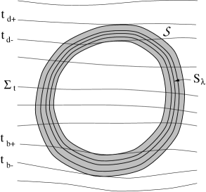
Figure 6: The support ${\cal S}$ of $\Sigma_{i}$ and $F^{i}$ in the 2-sphere solution is shown schematically, as are the 2-spheres $S_{\lambda}$ and the slicing $\Sigma_{t}$ used in the discussion of the phases of evolution of the 2-sphere solution.

The pre-birth phase is quite featureless. Since ${\cal S}_{t}=\emptyset$ for $t<t_{b-}$, $\tilde{w}^{a}=0$, so there is no $\tilde{E}$ or $\tilde{B}$ field. The evolution, which consists purely of $SO(3)$ gauge transformations of the pure gauge $A^{i}_{a}$ field, is generated by the Hamiltonian $H_{o}=-\int_{\Sigma}A^{i}_{0}D_{a}\tilde{E}^{a}_{i}$.

During the lifetime $\tilde{E}$ and $\tilde{B}$ also evolve quite straightforwardly. $\tilde{w}^{a}$ is a divergenceless vector density field living in the torus ${\cal S}_{t}$, defining ‘field lines’ filling this torus. One of the tangent vectors to $S_{\lambda}$, say $t_{2}$, may be taken to be spatial, i.e. to lie along the intersection $\gamma_{\lambda,t}=S_{\lambda}\cap\Sigma_{t}$. But then $0=t_{2}^{\mu}\sigma_{\mu b}=t_{2}^{a}\sigma_{ab}=\frac{1}{2}\epsilon_{abc}t_{2}^{a}\tilde{w}^{c}$, implies that $\tilde{w}^{a}$ lies along $t_{1}^{a}$. The ‘field lines’ of $\tilde{w}$ exactly trace the intersection curves $\gamma_{\lambda,t}$. In fact

$$\tilde{w}^{a}=\int_{\Box}d^{2}\lambda\ {}_{\scriptscriptstyle 3}\Delta^{a}_{\gamma_{\lambda,t}}(x)$$ (194)

where ${}_{\scriptscriptstyle 3}\Delta^{a}_{\gamma}=\int_{\gamma}\delta^{3}(x-z)\ dz^{a}$ is the characteristic distribution of the curve $\gamma$, in three dimensions.

Proof:

$$\tilde{w}^{a}(x)=\epsilon^{abc}\sigma_{bc}=2\int_{\Box}d^{2}\lambda\ \Delta^{0a}_{S_{\lambda}}(x,t)$$ (195)

$\Delta^{0a}_{S_{\lambda}}(x,t)=\int_{S_{\lambda}}\delta(t-z^{0})\delta^{3}(x-z)\ \frac{\partial z^{[0}}{\partial\sigma^{1}}\frac{\partial z^{a]}}{\partial\sigma^{2}}\ d^{2}\sigma$, where $\sigma^{A}$ are coordinates on $S_{\lambda}$. By choosing $\sigma^{1}=z^{0}$ (which can be done since the time, $z^{0}$, has no stationary points on $S_{\lambda}$ during ‘life’) we see that $\Delta^{0a}_{S_{\lambda}}=\frac{1}{2}\int_{\gamma_{\lambda,t}}\delta^{3}(x-z)dz^{a}=\frac{1}{2}{}_{\scriptscriptstyle 3}\Delta^{a}_{\gamma_{\lambda,t}}$, and (194) follows. 

Keeping the choice of coordinate $\sigma^{1}=z^{0}$ on $S_{\lambda}$ take as $t_{1}\$ $\frac{\partial}{\partial\sigma^{1}}$. Then $t_{1}^{0}=1$ and $\sigma_{0a}=-t_{1}^{b}\sigma_{ba}=-\frac{1}{2}\epsilon_{abc}\tilde{w}^{b}t_{1}^{c}$. This gives us a $\Sigma_{i\,0a}$ of the lapse-shift form (81):

$$\Sigma_{i\,0a}=e_{i}\sigma_{0a}=\frac{1}{2}\epsilon_{abc}\tilde{E}^{b}_{i}N^{c},$$ (196)

where $N^{c}=-t_{1}^{c}$.

Evolution is thus generated by

$$H_{l}=-\int_{\Sigma}A_{0}^{i}D_{a}\tilde{E}^{a}_{i}+\frac{1}{2}\epsilon_{abc}\tilde{B}^{i\,a}\tilde{E}^{b}_{i}N^{c}\ d^{3}x,$$ (197)

which, like $H_{o}$, is a special case of the Ashtekar Hamiltonian.

$\tilde{E}$ and $\tilde{B}$ evolve only by spatial diffeomorphisms, as can be seen by evolving with $H_{l}$ or, more simply, from the evolution (175) of $\tilde{w}$.

$$\dot{\tilde{w}}^{a} = 2\ \partial_{b}\sigma_{0c}\ \epsilon^{abc}$$ (200)

$$= 2\partial_{b}[\tilde{w}^{[a}N^{b]}]$$ (201)

$$= N^{b}\partial_{b}\tilde{w}^{a}+\tilde{w}^{a}\partial_{b}N^{b}-\partial_{b}N^{a}\tilde{w}^{b}$$ (202)

$$= \pounds_{\vec{N}}\ \tilde{w}^{a},$$ (203)

which then implies $\dot{\tilde{E}}^{a}_{i}=\pounds_{\vec{N}}\>\tilde{E}^{a}_{i}$ and $\dot{\tilde{B}}^{i\,a}=\pounds_{\vec{N}}\>\tilde{B}^{i\,a}$, since $e_{i}$ and $b^{i}$ are constant.

The most interesting aspect of the 2-sphere solution is the birth. During the birth there are points in ${\cal S}_{t}$ at which an $S_{\lambda}$ touches $\Sigma_{t}$ tangentially, and thus both $t_{1}$ and $t_{2}$ are spatial.

Generically such points form a line in $\Sigma_{t}$, but, by chosing a suitable slicing, $t_{1}$ and $t_{2}$ can be made spatial in the slices, ${\cal B}_{t}={\cal B}\cap\Sigma_{t}$, of an open set $\cal B$ in spacetime. For conceptual simplicity let us assume for the moment that such a slicing has been chosen. Then, in ${\cal B}_{t}$, $\tilde{w}^{a}=0$, while $\sigma_{0a}\neq 0$ but is proportional to $\epsilon_{abc}t_{1}^{b}t_{2}^{c}$. In fact $\sigma_{0a}$ is just the dual of the average over $\lambda_{A}$ of the characteristic distributions of the $S_{\lambda}$, which are tangent to the $\Sigma_{t}$ in $\cal B$. That is, in ${\cal B}_{t}$

$$\sigma_{0a}(x)=\bar{\sigma}_{0a}(x) = \frac{1}{2}\epsilon_{abc}\int_{\Box}d^{2}\lambda\ \Delta_{S_{\lambda}\cap{\cal B}}^{bc}(x,t)$$ (204)

$$= \frac{1}{2}\int_{\bf R}d\eta\ f(\eta)\ {}_{\scriptscriptstyle 3}\Delta^{bc}_{S_{\eta,t}}(x).$$ (205)

Here $\eta=g(\lambda)$ is chosen so that $\eta$ and $t_{min}$, the minimum of $t$ on a surface, parametrize the surfaces $\{S_{\lambda}\}$, $S_{\eta,t}=S_{\lambda(\eta,t_{min})}\cap{\cal B}_{t}$, and $f(\eta)=\int_{\Box}d^{2}\lambda\ \delta(t-z^{0}(\lambda))\delta(\eta-g(\lambda))$ is essentially a Jacobian. Note that in ${\cal B}$ $\ z^{0}$ depends only on $\lambda$, since the $S_{\lambda}$ are tangent to the $\Sigma_{t}$ there. Figure 7 illustrates the slicing and the $S_{\eta,t}$.

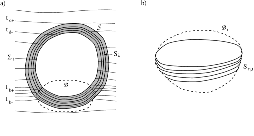
Figure 7: Panel a) shows the special slicing in which the initial equal time slices of the 2-spheres $S_{\lambda}$ are finite patches $S_{\eta,t}$ of 2-surface, and consequently flux loops are born with finite size. Panel b) shows the 3-volume ${\cal B}_{t}={\cal B}\cap\Sigma_{t}$ and the patches $S_{\eta,t}$ of the $S_{\lambda}$ in ${\cal B}_{t}$.

In ${\cal B}_{t}$ $\ \Sigma_{i\,0a}=\beta_{i\,a}\equiv e_{i}\bar{\sigma}_{0a}$, which is not of the lapse-shift form (81), and hence contributes a term to the Hamiltonian,

$$\Delta H_{b}=-\int_{\Sigma}\beta_{i\,a}\tilde{B}^{i\,a},$$ (206)

which is not present in $H_{Ash}$. Note that $\Delta H_{b}$ is independent of $\tilde{E}$, which is zero in ${\cal B}_{t}$.

Outside ${\cal B}_{t}$ $\ \Sigma_{i\,0a}$, and thus the Hamiltonian density, is of the same form as in the ‘life’ interval $(t_{b+},t_{d-})$. The total Hamiltonian during the birth is thus

$$H_{b}=\Delta H_{b}+H_{l}.$$ (207)

Now let’s consider evolution during the birth. $\Delta H_{b}$ contributes to the evolution of $\tilde{E}$

$$\Delta\dot{\tilde{E}}^{a}_{i} = 2\epsilon^{abc}D_{b}\beta_{i\,c}$$ (208)

$$= 2\epsilon^{abc}e_{i}\ \partial_{b}\bar{\sigma}_{0c}+2\epsilon^{abc}D_{b}e_{i}\ \bar{\sigma}_{0c}$$ (209)

$$= 2\int d\eta\ f(\eta)\ [e_{i}\partial_{b}\ {}_{\scriptscriptstyle 3}\Delta^{ab}_{S_{\eta,t}}+D_{b}e_{i}\ {}_{\scriptscriptstyle 3}\Delta^{ab}_{S_{\eta,t}}]$$ (210)

$$= \int d\eta\ f(\eta)\ e_{i}\ {}_{\scriptscriptstyle 3}\Delta^{a}_{\partial S_{\eta,t}}.$$ (211)

$\Delta H_{b}$ thus generates the birth of $\tilde{E}$ field lines $e_{i}\ {}_{\scriptscriptstyle 3}\Delta^{a}_{\partial S_{\eta,t}}$ at the boundary of ${\cal B}_{t}$, or, more specifically along the edges of the $S_{\eta,t}$, the pieces of the surfaces $S_{\lambda}$ lying in $\Sigma_{t}$. The second term in (210) vanishes because $e_{i}$ is covariantly constant on the 2-surfaces $S_{\lambda}$, and thus on $S_{\eta,t}$.

Equivalently, the second term in (209) can be shown to vanish in a more elementary, if less picturesque, way using the constancy of $e_{i}$ and (172), which implies that $\alpha_{b}\sigma_{0c}\epsilon^{abc}=0$ because $\tilde{w}^{a}=0$. Similarly the characteristics of the surviving contribution to $\Delta\dot{\tilde{E}}$, $e_{i}\>\epsilon^{abc}\partial_{b}\bar{\sigma}_{0c}$, can be derived from (175). Since $\dot{\tilde{w}}$ vanishes inside ${\cal B}_{t}$ and $\bar{\sigma}_{0c}$ vanishes outside $\tilde{u}^{a}\equiv 2\epsilon^{abc}\partial_{b}\bar{\sigma}_{0c}$ lives on the boundary of ${\cal B}_{t}$. Moreover $\partial_{a}\tilde{u}^{a}=0$, so $\Delta\dot{\tilde{E}}_{i}^{a}=e_{i}\ \tilde{u}^{a}$ shows, like our previous analysis, that $\Delta H_{b}$ generates the birth of $\tilde{E}$ field lines along the boundary of ${\cal B}_{t}$.

$\Delta H_{b}$ also generates an entirely analogous evolution of the $\tilde{B}$ field that ensures that along with the $\tilde{E}$ field lines are born corresponding $\tilde{B}$ field lines so that (3) is satisfied. The $H_{l}$ term in $H_{b}$ then generates a 3-diffeomorphism that moves the field lines (initially) away from $\partial{\cal B}_{t}$.

In summary, the $\tilde{E}$ and $\tilde{B}$ fields evolve as follows in the 2-sphere solution: Until birth begins $\tilde{E}$ and $\tilde{B}$ are zero. During birth loops of $\tilde{E}$ and $\tilde{B}$ flux, i.e. field lines, are generated by $\Delta H_{b}$. As they are created these field lines move out, forming a torus in space once the birth is completed. This torus expands and recontracts, and then the events of the birth are repeated in reverse during death, leaving ultimately $\tilde{E}=\tilde{B}=0$.

In a generic slicing a given $S_{\lambda}$ and $\Sigma_{t}$ will be tangent only if $t_{min}$ (or $t_{max}$) of $S_{\lambda}$ coincides with $t$, and then only at one point. In other words, the ‘disks’ $S_{\eta,t}$ are points in a generic slicing. The union, over $\lambda_{1}$ and $\lambda_{2}$ of these points of tangency to a fixed $\Sigma_{t}$ then forms a line $\ell$ in $\Sigma_{t}$.

I have used Ashtekar’s Hamiltonian density (which is correct when $\Sigma_{i\,0a}$ is of the lapse-shift form) outside ${\cal B}_{t}$ to emphasize that the evolution there is the same as in Ashtekar’s theory. This approach becomes confusing when the $S_{\eta,t}$ are points. It is then better to treat all of $\Sigma$ uniformly by using the Hamiltonian density $\tilde{\cal H}_{\Sigma}=-A^{i}_{0}D_{a}\tilde{E}^{a}_{i}-\Sigma_{i\,0a}\,[\tilde{B}^{i\,a}-\phi^{ij}\tilde{E}^{a}_{j}]$ everywhere, treating $\Sigma_{i\,0a}$ as independent of $A$ and $\tilde{E}$ in the Poisson brackets, and only afterward substituting the particular form of $\Sigma_{i\,0a}$ into the resulting evolution equation. The occurrence of births and deaths is then indicated by $\Sigma_{i\,0a}\neq 0$ at some points where $\tilde{E}=0$.

We can conclude that the crucial feature of the new Hamiltonian of Section 4 which lets it, unlike Ashtekar’s Hamiltonian, generate births and deaths is the presence of $\tilde{E}$ independent contributions

$$\Delta\tilde{\cal H}_{b}=\beta_{i\,a}\tilde{B}^{i\,a},$$ (212)

where $\beta_{i\,a}$ may be non-zero when $\tilde{E}=0$. The Ashtekar Hamiltonian contains only terms that are positive powers of $\tilde{E}$, so $\{\tilde{E}^{a}_{i},H_{Ash}\}=0$ when $\tilde{E}=0$. $H_{Ash}$ can only generate changes in $\tilde{E}$ in the support of $\tilde{E}$ or its boundary.

Appendix A Faraday lines as the classical limit of graph basis states

In this Appendix it is shown that, in the classical limit, the graph basis state $|\gamma,j\rangle$ associated with a graph consisting of an intersection free loop $\gamma$, carrying spin $j$, essentially represents an isolated line of $\tilde{E}$ flux along $\gamma$. (The result trivially generalizes to the graph basis states corresponding to disjoint collections of such loops.)

More precisely, $|\gamma,j\rangle$ can be written as the sum of two states $|\gamma,j\rangle^{+}$ and $|\gamma,j\rangle^{-}$ such that, in the connection representation (see [Ash91]) in which the operator $\hat{A}^{i}_{a}$ acts by multiplication,

$$\langle A|\hat{\tilde{E}}^{a}_{i}|\gamma,j\rangle^{+} = \tilde{E}_{(\gamma,j)}{}^{a}_{i}\langle A|\gamma,j\rangle^{+}+O(\hbar)$$ (213)

$$\langle A|\hat{\tilde{E}}^{a}_{i}|\gamma,j\rangle^{-} = -\tilde{E}_{(\gamma,j)}{}^{a}_{i}\langle A|\gamma,j\rangle^{-}+O(\hbar),$$ (214)

with

$$\tilde{E}_{(\gamma,j)}{}^{a}_{i}=e_{i}\>{}_{\scriptscriptstyle 3}\Delta^{a}_{\gamma},$$ (215)

${}_{\scriptscriptstyle 3}\Delta^{a}_{\gamma}(x)=\int_{\gamma}\delta^{3}(x-z)dz^{a}$, and $e_{i}=j\hbar n_{i}$, where the unit $SO(3)$ vector $n_{i}$ is covariantly constant on $\gamma$. Unless, that is, the holonomy of $A$ around $\gamma$ is ${\bf 1}$. Notice that when the holonomy is not ${\bf 1}$ all covariantly constant vectors on $\gamma$ are constant multiples of $n$, so $\tilde{E}_{(\gamma,j)}{}$ is uniquely defined, up to sign, by $\gamma$, $j$, and $A$.

As $\hbar$ becomes small $\langle A|\hat{\tilde{E}}^{a}_{i}|\gamma,j\rangle^{\pm}\rightarrow 0$ unless $j\sim O(1/\hbar)$, in which case $e_{i}$ is finite and (215) is an isolated Faraday line carrying flux $e_{i}$. Thus, according to our claim $|\gamma,j\rangle$ in fact represents two Faraday lines, of opposite flux, along $\gamma$.

Let’s prove the claim (213), (214).

In the connection representation the graph basis state $|\gamma,j\rangle$ is represented by [Rei94]

$$\langle A|\gamma,j\rangle=trH^{(j)}[A,\gamma],$$ (216)

(times a normalization $\sqrt{2j+1}$ which will be dropped here). $H^{(j)}[A,\gamma]={\cal P}\>exp(\int_{\gamma}A^{i}J_{i}^{(j)})$ is the spin $j$ holonomy around $\gamma$, and the $J_{i}^{(j)}$ are the spin $j$ representations of the antihermitian $su(2)$ generators. In other words $\langle A|\gamma,j\rangle$ is the spin $j$ Wilson loop.

Now the result (213), (214) can be derived by straightforward mathematics. The holonomy referred to the base point $p\in\gamma$ can be written as

$$H^{(j)}_{p}[A,\gamma]=e^{\theta^{i}(p)J_{i}^{(j)}}.$$ (217)

Its trace (which is independent of $p$) is

$$tr[e^{\theta^{i}(p)J_{i}^{(j)}}] = \sum_{m=-j}^{j}e^{i|\theta|m}$$ (218)

$$= \frac{\sin(j+\frac{1}{2})|\theta|}{\sin\frac{1}{2}|\theta|}$$ (219)

$$= c(|\theta|)e^{i|\theta|j}+c(|\theta|)^{*}e^{-i|\theta|j},$$ (220)

where $c(|\theta|)=\frac{1}{2}[1-i\cot\frac{|\theta|}{2}]$.

It is easy to show that $\theta^{i}(p)$ is covariantly constant on $\gamma$, and that its magnitude is $|\theta|=\int_{\gamma}n_{i}A^{i}$, where $n_{i}$ is the $SO(3)$ unit vector $\theta_{i}/|\theta|$. Thus

$$\langle A|\gamma,j\rangle=c(|\theta|)e^{i\int_{\gamma}n_{i}A^{i}j}+c(|\theta|)^{*}e^{-i\int_{\gamma}n_{i}A^{i}j}.$$ (221)

Taking

$$\langle A|\gamma,j\rangle^{+} = c(|\theta|)e^{i\int_{\gamma}n_{i}A^{i}j}$$ (222)

$$\langle A|\gamma,j\rangle^{-} = c(|\theta|)^{*}e^{-i\int_{\gamma}n_{i}A^{i}j}$$ (223)

we find (213) and (214):

$$\langle A|\hat{\tilde{E}}^{a}_{i}|\gamma,j\rangle^{+} \equiv -i\hbar\frac{\delta}{\delta A^{i}_{a}}\langle A|\gamma,j\rangle^{+}$$ (224)

$$= [j+\frac{\partial}{\partial|\theta|}\log c(|\theta|)]\hbar n_{i}\int_{\gamma}\delta^{3}(x-z)dz^{a}\langle A|\gamma,j\rangle^{+}$$ (225)

$$= \tilde{E}_{(\gamma,j)}{}^{a}_{i}\langle A|\gamma,j\rangle^{+}+O(\hbar).$$ (226)

(214) follows similarly.

$\tilde{E}_{(\gamma,j)}{}^{a}_{i}=e_{i}{}_{\scriptscriptstyle 3}\Delta^{a}_{\gamma}$ might not seem like a proper eigenvalue field, even in the classical limit, because $e_{i}$ depends on $A$, the argument of $\langle A|\gamma,j\rangle$. However, by a gauge transformation one can always make $n_{i}=\delta^{3}_{i}$ on all of $\gamma$, leading to

$$\tilde{E}_{(\gamma,j)}{}^{a}_{i}={}_{0}\tilde{E}_{(\gamma,j)}{}^{a}_{i}\equiv j\hbar\delta^{3}_{i}{}_{\scriptscriptstyle 3}\Delta^{a}_{\gamma},$$ (227)

which is manifestly independent of $A$. While the components of $\tilde{E}_{(\gamma,j)}{}$ depend on gauge, they do not depend on the gauge equivalence class of the $A$ field, which is the true argument of the gauge invariant functions $\langle A|\gamma,j\rangle^{\pm}$. Hence, in a suitable gauge fixing $|\gamma,j\rangle^{\pm}$ is, when $\hbar\rightarrow 0$, an eigenstate of $\hat{\tilde{E}}^{a}_{i}$ with eigenvalue $\pm{}_{0}\tilde{E}_{(\gamma,j)}{}^{a}_{i}$. So $|\gamma,j\rangle^{\pm}$ represent, in the classical limit, Faraday lines, which are described in an arbitrary gauge by $\tilde{E}^{a}_{i}=\pm\tilde{E}_{(\gamma,j)}{}$.

Appendix B Tetrads from bases of self-dual 2-forms

A proof is given of a somewhat elaborated form of a theorem of Capovilla, Dell, Jacobson and Mason [CDJM91]. The very efficient proof given in [CDJM91] relies on spinorial techniques. Here $SO(3)$ tensors are used.

Theorem

$$\Sigma_{i}\wedge\Sigma_{j}=\frac{1}{3}\delta_{ij}\Sigma_{k}\wedge\Sigma^{k}$$ (228)

$$\Sigma_{i}\wedge\Sigma^{i}\neq 0,$$ (229)

1), implies that there exists a non-singular co-tetrad $e^{I}{}_{\mu}$ such that

$$\Sigma_{i}=\frac{1}{2}e^{0}\wedge e^{i}+\frac{1}{4}\epsilon_{ijk}e^{j}\wedge e^{k}.$$ (230)

Furthermore,

2), the metric $g_{\mu\nu}=e^{I}{}_{\mu}\delta_{IJ}e^{J}{}_{\nu}$ is uniquely determined by $\Sigma_{i}$, and is in fact equal to the Urbantke metric [Urb83] defined by

$$\sqrt{g}g_{\mu\nu}=4\Sigma_{1\,\mu\alpha}\Sigma_{2\,\beta\gamma}\Sigma_{3\,\delta\nu}\epsilon^{\alpha\beta\gamma\delta}.$$ (231)

3), $e_{0}{}^{\mu}$ may be chosen to be any unit vector of $g$ ($e_{I}{}^{\mu}$ is the inverse of $e^{I}{}_{\mu}$), but once this vector is chosen $e^{I}{}_{\mu}$ is uniquely determined. Equivalently, $e^{I}{}_{\mu}$ is unique up to the action of the $SO(3)_{R}$ subgroup of $SO(4)$ on the internal index $I$.

4), When $\Sigma_{i}$ is real there exist either real $e^{I}{}_{\mu}$ satisfying (230), corresponding to a positive definite metric, or pure imaginary $e^{I}{}_{\mu}$, corresponding to a negative definite metric.

Proof:

First let’s establish 1) by constructing a cotetrad $e^{I}{}_{\mu}$ satisfying (230). Any vector $t^{\mu}$ allows us to define three 1-forms

$$f^{i}{}_{\mu}=2t^{\sigma}\Sigma_{i\,\sigma\mu}.$$ (232)

These will ultimately, after a rescaling, serve as the ‘spatial’ part, $e^{i}{}_{\mu}$ of $e^{I}{}_{\mu}$.

When $t$ and the $\Sigma_{i}$ are real the $f^{i}$ are easily shown to be linearly independent: if they were not there would exist non-zero, real $a_{i}$ such that $a_{i}f^{i}=0$. This implies $t^{\sigma}[a^{i}\Sigma_{i}]_{\sigma\mu}=0$, which means that $rank[a^{i}\Sigma_{i}]=2$ or $0$, implying, in turn, that

$$0=a^{i}\Sigma_{i}\wedge a^{j}\Sigma_{j}=a^{i}a^{j}\frac{1}{3}\delta_{ij}\Sigma_{k}\wedge\Sigma^{k}.$$ (233)

Since $\Sigma_{k}\wedge\Sigma^{k}\neq 0$ this requires $\delta_{ij}a^{i}a^{j}=0\Rightarrow a^{i}=0$. That is, the $f^{i}$ are linearly independent.

If the $\Sigma_{i}$ and/or $t$ are complex the situation is less simple. The $f^{i}$ may then be complex and linear dependence requires only the existence of non-zero complex $a^{i}$ such that $a_{i}f^{i}=0$. Now $\delta_{ij}a^{i}a^{j}=0$ has non-zero complex solutions. By (233), if $a^{i}$ is such a solution $rank[a^{i}\Sigma_{i}]=2$. ($rank[a^{i}\Sigma_{i}]=0$, i.e. $a^{i}\Sigma_{i}=0$, is excluded because this would imply $0=a^{i}\Sigma_{i}\wedge\Sigma_{j}=a_{j}(\frac{1}{3}\Sigma_{k}\wedge\Sigma^{k})\rightarrow a_{j}=0$.) If $t$ is chosen to be a null vector of $a^{i}\Sigma_{i}$ then the corresponding $f^{i}$ will not be linearly independent.

Nevertheless, it will now be shown that there are $t$ with $f^{i}$ that are independent. Let $N_{3}\subset{\bf C}^{3}$ be the set of solutions to $\delta_{ij}a^{i}a^{j}=0$, and let $N_{4}=\{t\in{\bf C}^{4}|\exists a\in N_{3}\ni t^{\mu}[a^{i}\Sigma_{i}]_{\mu\nu}=0\}$. $N_{4}$ is the set of $t$ having linearly dependent $f^{i}$. $N_{4}$ can be thought of as the subset of ${\bf C}^{4}$ swept out by the two dimensional null plane of $a^{i}\Sigma_{i}$ as $a$ ranges over $N_{3}$. $N_{3}$ is a two dimensional cone in ${\bf C}^{3}$, but one of these dimensions corresponds to rescalings of $a$, which do not affect the null plane of $a^{i}\Sigma_{i}$. Thus $N_{4}$ has, at most, dimension $2+1=3$. This makes it a lower dimensional subset of ${\bf C}^{4}$ so ${\bf C}^{4}-N_{4}$ is not empty. It will be shown below that $N_{4}$ is the null cone of the metric induced by $\Sigma_{i}$.

Choose any $t\in{\bf C}^{4}-N_{4}$. The corresponding $f^{i}$ are linearly independent. Furthermore, $t^{\mu}f^{i}{}_{\mu}=0$ so, if $\alpha$ is a 1-form such that $t^{\mu}\alpha_{\mu}=1$, $\{\alpha,f^{i}\}$ form a basis of 1-forms, which can be used to expand the $\Sigma_{i}$. Taking (232) into account

$$\Sigma_{i}=\frac{1}{2}\alpha\wedge f^{i}+\beta_{ijk}f^{j}\wedge f^{k},$$ (234)

with $\beta_{ijk}$ antisymmetric in $j\>k$.

Using this expansion we may write

$$\Sigma_{i}\wedge\Sigma_{j} = \frac{1}{2}\beta_{jlm}\alpha\wedge f^{i}\wedge f^{l}\wedge f^{m}+\frac{1}{2}\beta_{ilm}f^{l}\wedge f^{m}\wedge\alpha\wedge f^{j}$$ (235)

$$= \epsilon^{lm}{}_{(i}\beta_{j)lm}\alpha\wedge f^{1}\wedge f^{2}\wedge f^{3}.$$ (236)

(228) then implies $\epsilon^{lm}{}_{(i}\beta_{j)lm}\propto\delta_{ij}$, that is,

$$\epsilon^{lm}{}_{i}\beta_{jlm}=\kappa\delta_{ij}+\eta^{k}\epsilon_{ijk}$$ (237)

for some $\kappa\neq 0$ and $\eta^{i}$ ((229) implies $\kappa\neq 0$). Now, since $\beta_{ijk}$ is antisymmetric in $j\>k$,

$$\beta_{ijk}=\frac{1}{2}\epsilon^{n}{}_{jk}[\epsilon^{lm}{}_{n}\beta_{ilm}]=\frac{1}{2}\kappa\epsilon_{ijk}+\delta_{i[j}\eta_{k]}.$$ (238)

Hence,

$$\Sigma_{i} = \frac{1}{2}[\alpha-2\eta_{k}f^{k}]\wedge f^{i}+\frac{1}{2}\kappa\epsilon_{ijk}f^{j}\wedge f^{k}$$ (239)

$$= 2\kappa[\frac{1}{2}f^{0}\wedge f^{i}+\frac{1}{4}\epsilon_{ijk}f^{j}f^{k}],$$ (240)

with $f^{0}=\frac{1}{2\kappa}(\alpha-2\eta_{k}f^{k})$. To arrive at the form (230) of $\Sigma_{i}$ it is simply necessary to absorb the factor $2\kappa$ in a rescaling of the basis 1-forms: let

$$e^{I}{}_{\mu}=\sqrt{2\kappa}f^{I}{}_{\mu}$$ (241)

then

$$\Sigma_{i}=\frac{1}{2}e^{0}\wedge e^{i}+\frac{1}{4}\epsilon_{ijk}e^{j}\wedge e^{k}.$$ (242)

This proves 1).

Now for 2). $e^{I}{}_{\mu}$ determines a spacetime metric $g_{\mu\nu}=e^{I}{}_{\mu}\delta_{IJ}s^{J}{}_{\nu}$. The formulas

$$[det\ e]g_{\mu\nu} = 4\Sigma_{1\,\mu\alpha}\Sigma_{2\,\beta\gamma}\Sigma_{3\,\delta\nu}\epsilon^{\alpha\beta\gamma\delta}$$ (243)

$$det\ e = \frac{1}{6}\Sigma_{i\,\alpha\beta}\Sigma^{i}_{\gamma\delta}\epsilon^{\alpha\beta\gamma\delta}\neq 0$$ (244)

can be verified by substituting the expansion (230) for the $\Sigma_{i}$. Together they show that $g_{\mu\nu}$ is determined by the $\Sigma_{i}$.

3). How unique is $e^{I}{}_{\mu}$? First note that $e^{I}{}_{\mu}$ is the $f^{I}{}_{\mu}$ corresponding to a normalized $t^{\mu}$, namely $t_{0}^{\mu}=\sqrt{2\kappa}t^{\mu}$. Since $t_{0}^{\mu}e^{I}{}_{\mu}=\delta^{I}_{0}$ $t_{0}^{\mu}=e_{0}{}^{\mu}$, the ‘time’ element of $e_{I}{}^{\mu}$, the inverse $e^{I}{}_{\mu}$.

Now let’s suppose we are given a cotetrad $e^{\prime I}{}_{\mu}$ satisfying (230). Are there distinct $e^{I}{}_{\mu}$, also satisfying (230), with $e_{0}{}^{\mu}$ pointing in the same direction as $e^{\prime}_{0}{}^{\mu}$? Take $t^{\mu}=\lambda e^{\prime}_{0}{}^{\mu}$ with $\lambda>0$.

$$f^{i}{}_{\mu}=2t^{\sigma}\Sigma_{i\,\sigma\mu}=\lambda e^{\prime i}{}_{\mu}.$$ (245)

These $f^{i}$ are linearly independent, so $t\in{\bf C}^{4}-N_{4}$. Thus $\Sigma_{i}$ can be expanded according to (240) in $f^{I}\wedge f^{J}$ and according to (230) in $e^{\prime}I\wedge e^{\prime J}$. Making use of (245) we find

$$2\kappa[\frac{1}{2}f^{0}\wedge\lambda e^{\prime i}+\frac{1}{4}\lambda^{2}\epsilon_{ijk}e^{\prime j}\wedge e^{\prime k}]=\frac{1}{2}e^{\prime 0}\wedge e^{\prime j}+\frac{1}{4}\epsilon_{ijk}e^{\prime j}\wedge e^{\prime k}$$ (246)

The linear independence of the $e^{\prime}I\wedge e^{\prime J}$ now demands $2\kappa=1/\lambda^{2}$ and $\frac{1}{\lambda}f^{0}\wedge e^{\prime i}=e^{\prime 0}\wedge e^{\prime i}$ - which implies $f^{0}=\lambda e^{\prime 0}$. Hence

$$e^{I}{}_{\mu}=\sqrt{2\kappa}f^{I}{}_{\mu}=\frac{1}{\lambda}\lambda e^{\prime}I{}_{\mu}=e^{\prime}I{}_{\mu}.$$ (247)

The cotetrads $e^{I}{}_{\mu}$ satisfying (230) are thus in one to one correspondence with the rays of vectors $t\in{\bf C}^{4}-N_{4}$.

Note that $e_{0}{}^{\mu}$ cannot lie in the null cone ${\cal C}\subset{\bf C}^{4}$ of the metric $g$, since $e^{0}{}_{\mu}=g_{\mu\nu}e_{0}{}^{\nu}$ has to be a unit vector and finite. Thus ${\cal C}\subset N_{4}$.

Note also that $\Sigma_{i}=[e\wedge e]^{+i}$, a self-dual component of $e^{I}\wedge e^{J}$. The $\Sigma_{i}$ are therefore invariant under anti-self-dual $SO(4)$ (i.e. $SO(3)_{R}$) transformations on the internal index $I$ of $e^{I}{}_{\mu}$. It follows from the anti-self-duality of the generators of $SO(3)_{R}$ that $SO(3)_{R}$ transformations consist of an $SO(4)$ boost by an arbitrary rapidity $\theta^{i}$, accompanied by a spatial rotation by an angle $|\theta|$ about $\theta^{i}$. Hence $e_{0}{}^{\mu}$ can be boosted to be parallel to any given unit vector $t_{0}^{\mu}$, provided the rest of the tetrad is rotated apropriately. (Note that $e^{I}\rightarrow-e^{I}$ is in $SO(3)_{R}$, so $SO(3)_{R}$ will take $e_{0}$ from the past to the future unit norm shell in the Lorentzian section, though via a path that departs from this section at intermediate points). We see that there is an $e^{I}{}_{\mu}$ corresponding to each $t\in{\bf C}^{4}-{\cal C}$, so $N_{4}={\cal C}$. Furthermore, we see that all $e^{I}{}_{\mu}$ are $SO(3)_{R}$ transforms of one $e^{I}{}_{\mu}$. Thus the freedom in $e^{I}{}_{\mu}$ for given $\Sigma_{i}$ is precisely $SO(3)_{R}$.

4), the case of real $\Sigma_{i}$.

If $t^{\mu}$ is taken to be real then the $f^{i}$ are real, $\kappa$ is real, and, if $\alpha$ is taken to be real, $\eta^{i}$ is real. Hence the $f^{I}$ are real in this case. However, $\kappa$ can be positive or negative, leading to either real $e^{I}$ and a positive definite metric, or pure imaginary $e^{I}$ and a negative definite metric. 

Appendix C The case $rank\tilde{E}=2$

In this appendix it is shown that when $\tilde{E}$ is degenerate but of rank $2$ Ashtekar’s constraints are still equivalent to the new constraints (2) and (3), and $\Sigma_{i\,0a}$ is of the lapse-shift form (81).

When $rank\tilde{E}=2$ both the internal span of $\tilde{E}^{a}_{i}$ (the span of $\tilde{E}^{a}_{i}$ seen as three internal vectors labeled by $a$), and its external span, are two dimensional. Therefore there exists an internal vector $v^{i}$ and an external vector $w_{a}$ such that $v^{i}\tilde{E}_{i}^{a}=w_{a}\tilde{E}_{i}^{a}=0$. Note also that $\tilde{\varepsilon}^{i}_{a}=\frac{1}{2}\epsilon^{ijk}\epsilon_{abc}\tilde{E}^{b}_{j}\tilde{E}^{c}_{k}\propto v^{i}w_{a}$, and is non-zero.

Let’s first show that Ashtekar’s constraints (2), (4), and (5) imply the full constraints, (2) and (3). The Gauss law constraint (2) is the same in both sets, so it remains only to show that the vector and scalar constraints, (4) and (5), imply (3).

The vector constraint implies

$$\epsilon_{ijk}\tilde{B}^{i\,a}\tilde{\varepsilon}^{j}_{a}=0,$$ (248)

and the scalar constraint can be written as

$$\delta_{ij}\tilde{B}^{i\,a}\tilde{\varepsilon}^{j}_{a}=0.$$ (249)

(248) and (249) require that $\psi^{ij}=\tilde{B}^{i\,a}\tilde{\varepsilon}^{j}_{a}$ be trace free and symmetric. On the other hand $\psi^{ij}\propto\tilde{B}^{i\,a}w_{a}v^{j}$, so it is rank $1$. Together these requirements imply that $\psi^{ij}=0$, which in turn implies that $\tilde{B}^{i\,a}w_{a}=0$. In other words, $\tilde{B}^{i\,a}$ is in the external span of $\tilde{E}$:

$$\tilde{B}^{i\,a}=\theta^{ij}\tilde{E}^{a}_{j}$$ (250)

for some $\theta$. Substituting (250) back into the vector constraint gives

$$0=\theta^{ij}\tilde{E}^{a}_{j}\tilde{E}^{b}_{i}\epsilon_{abc},$$ (251)

i.e. the component of $\theta$ acting in the internal span of $\tilde{E}$ is symmetric. From (250) it can be seen that the remaining components of $\theta$ may be chosen freely. $\theta$ may, therefore, be chosen trace free and symmetric. The constraint (3),

$$\exists\phi^{ij}\mbox{trace free, symmetric}\ni\tilde{B}^{i\,a}-\phi^{ij}\tilde{E}^{a}_{j}=0,$$ (252)

is thus satisfied.

Now let’s show that the general solution to the field equation (66),

$$\Sigma_{(i\,0a}\tilde{E}^{a}_{j)}\propto\delta_{ij},$$ (253)

is the lapse, shift form of $\Sigma_{i\,0a}$:

$$\Sigma_{i\,0a}=\frac{1}{4}N\epsilon_{i}{}^{jk}\epsilon_{abc}\tilde{E}^{b}_{j}\tilde{E}^{c}_{k}+\frac{1}{2}\epsilon_{abc}\tilde{E}^{b}_{i}N^{c}.$$ (254)

(253) always implies that

$$\Sigma_{i\,0a}\tilde{E}^{a}_{j}=\tilde{c}_{1}\delta_{ij}+\epsilon_{ikj}\tilde{c}_{2}^{k},$$ (255)

for some $\tilde{c}_{1}$ and $\tilde{c}_{2}$. When $rank\tilde{E}=2$ (255) can be simplified as follows. Contracting (255) with $v^{j}$ gives $0=\tilde{c}_{1}v_{i}+\epsilon_{ikj}\tilde{c}_{2}^{k}v^{j}$, which implies $\tilde{c}_{1}=0$ and $\tilde{c}_{2}\parallel v$. Thus

$$\Sigma_{i\,0a}\tilde{E}^{a}_{j}\propto\epsilon_{ikj}v^{k}.$$ (256)

The component of $\Sigma_{i\,0a}$ in the external span of $\tilde{E}$ has only one degree of freedom. The component transverse to the external span of $\tilde{E}$ is, of course, totally unconstrained by (253), and so has three degrees of freedom. This makes for a total of four degrees of freedom, which is exactly what the lapse, shift form (254) of $\Sigma_{i\,0a}$ has, a good sign.

(256) may be written as

$$\Sigma_{i\,0a}\tilde{E}^{a}_{j}=\frac{1}{4}\epsilon_{ikj}[\epsilon^{klm}\epsilon_{abc}\tilde{E}^{b}_{l}\tilde{E}^{c}_{m}]N^{a}=\frac{1}{2}\epsilon_{abc}\tilde{E}^{b}_{i}N^{c}\tilde{E}^{a}_{j},$$ (257)

in which only the component of $N$ along $w$ contributes. $\Sigma_{i\,0a}$ itself is thus of the form

$$\Sigma_{i\,0a}=\frac{1}{2}\epsilon_{abc}\tilde{E}^{b}_{i}N^{c}+c_{3\,i}w_{a}.$$ (258)

$c_{3\,i}$ captures the three degrees of freedom of the component of $\Sigma_{i\,0a}$ transverse to the external span of $\tilde{E}$. Note, however, that the components of $N$ transverse to $w$ contribute to (258), and that their contribution spans expressions of the form $c_{i}w_{a}$ with $c_{i}v^{i}=0$. Thus $c_{3}$ may be set parallel to $v$, making the last term in (258) proportional to $v_{i}w_{a}\propto\epsilon_{i}{}^{jk}\epsilon_{abc}\tilde{E}^{b}_{j}\tilde{E}^{c}_{k}$. (258) is then of the form (254).

Appendix D Characteristic distributions

Characteristic distributions can be defined for any $n$ dimensional submanifold, $M$, of a $d$ dimensional space:

$$\Delta_{M}^{\mu_{1}...\mu_{n}}=\int_{M}\delta^{d}(x-z)dz^{[\mu_{1}}...dz^{\mu_{n}]}.$$ (259)

These distributions have the important property that for an arbitrary $n$-form, $g$,

$$\int_{M}g=\int_{{\bf R}^{d}}\Delta_{M}^{\mu_{1}...\mu_{n}}g_{\mu_{1}...\mu_{n}}d^{d}x.$$ (260)

The $\Delta$’s of submanifolds and those of their boundaries are connected by the identity

$$\partial_{\mu_{1}}\Delta_{M}^{\mu_{1}\mu_{2}...\mu_{n}}=-\frac{1}{n}\Delta_{\partial M}^{\mu_{2}...\mu_{n}}.$$ (261)

(261) follows directly from Stokes theorem: for an arbitrary $n-1$-form $f$

$$\int_{{\bf R}^{d}}\partial_{\mu_{1}}\Delta_{M}^{\mu_{1}\mu_{2}...\mu_{n}}f_{\mu_{2}...\mu_{n}}d^{d}x = -\int_{{\bf R}^{d}}\Delta_{M}^{\mu_{1}...\mu_{n}}\partial_{[\mu_{1}}f_{\mu_{2}...\mu_{n}]}d^{d}x$$ (262)

$$= -\frac{1}{n}\int_{M}d\wedge f$$ (263)

$$= -\frac{1}{n}\int_{\partial M}f$$ (264)

$$= -\frac{1}{n}\int_{{\bf R}^{d}}\Delta_{\partial M}^{\mu_{2}...\mu_{n}}f_{\mu_{2}...\mu_{n}}d^{d}x,$$ (265)

the arbitrariness of $f$ implying (261).