Head-on collision of two black holes:
comparison of different approaches

Abstract

A benchmark problem for numerical relativity has been the head-on collision of two black holes starting from the “Misner initial data,” a closed form momentarily stationary solution to the constraint equations with an adjustable closeness parameter $\mu_{0}$. We show here how an eclectic mixture of approximation methods can provide both an efficient means of determining the time development of the initial data and a good understanding of the physics of the problem. When the Misner data is chosen to correspond to holes initially very close together, a common horizon surrounds both holes and the geometry exterior to the horizon can be treated as a non-spherical perturbation of a single Schwarzschild hole. When the holes are initially well separated the problem can be treated with a different approximation scheme, “the particle-membrane method.” For all initial separations, numerical relativity is in principle applicable, but is costly and of uncertain accuracy. We present here a comparison of the different approaches. We compare waveforms, for $\ell=2$ and $\ell=4$ radiation, for different values of $\mu_{0}$, from the three different approaches to the problem.

I Introduction

The advent of LIGO and VIRGO [1], and other gravitational radiation detectors in the coming years, adds motivation to achieve a better understanding of the physics of black hole collisions, physics that is already interesting for many other reasons. Not the least of these is that black hole collisions were the earliest testbed for numerical relativity, the solution of the differential equations of Einstein’s theory with numerical codes. Smarr and Eppley[2, 3, 4], more than 15 years ago, computed the radiation waveforms for the axisymmetric problem of two holes, starting from rest and falling into each other in a head-on collision. Partly to gauge the progress of the past 15 years, both in computing machinery and in its application to the problem, the problem has recently been reconsidered and recomputed[5, 6]. One of the reasons for the importance of this problem is that it is a starting point for a major initiative in state-of-the-art computing, the Grand Challenge project[7] to compute the spiraling coalescence of binary black hole systems in the absence of symmetries. This project will rely on both large scale numerical computations to solve the fully nonlinear Einstein equations and on a new set of semi-analytic techniques, such as those presented here, to gain a physical understanding of the numerical results and to provide testbed calculations to verify the new generation of numerical codes under development[8].

The technical difficulties of solving the dynamics of black hole interactions are daunting, as will be clear in the limits of progress reported below. The difficulties make it important, or even necessary, that the numerical work be supported by other approaches. In particular, the numerical challenge would be greatly aided by analytic or semi-analytic methods of computing black hole solutions in cases where such methods can be devised, so that those developing numerical codes would be guided. Most important, distinctly different methods of finding solutions can provide a measure of the errors, especially the systematic errors, in the numerical schemes.

There is a very separate motivation for developing alternative methods of finding solutions. While numerical treatment gives us the data representing the physical process, analytical methods provide a structure for understanding these data, for perceiving what is interesting, what is expected and is new, and what generalizations are plausible, and what questions should be asked next.

We report here on work done with just such motivations. The problem is the head-on collision of two holes, the classic problem of Smarr and Eppley. The initial data is the analytical solution of the Einstein initial value equations given by Misner[9]. This solution represents two symmetric, momentarily stationary, “throats” with a proper separation $L$, in a spacetime with ADM mass $M$ (thus representing two momentarily stationary holes each of mass roughly $M/2$)[10]. In this solution the dimensionless measure of initial separation $L/M$ of the throats is given by a parameter $\mu_{0}$.

Initial data with large values of $\mu_{0}$ represent infall scenarios starting from large separations. Small $\mu_{0}$ corresponds to very different collapses starting with close throats. Three distinctly different methods are used to study the problem: (i) Over a broad range of separations, the more-or-less established approach to numerical relativity, the numerical solution of the Einstein equations in 3+1 form, is used to find the spacetime evolved from the initial data. (ii) For large separations (“far limit”) we use the “particle-membrane” method, which starts with a point particle infall treated using perturbation theory, and then introduces factors describing the internal dynamics of the black holes, using the black hole membrane paradigm. (iii) In the “close limit,” when initial separations are small, we exploit the fact that the initial geometry is nearly spherical outside the initial horizon; the evolved spacetime outside the horizon is therefore nearly spherical and its development can be approximated with the theory of non-spherical perturbations of a single black hole.

The range of validity of the three methods is shown below and their strengths and weaknesses discussed. The conclusion that emerges is that the eclectic approach to this problem, using a mixture of distinctly different computational methods, gives a very robust set of answers, with good limits on errors, and much improved understanding of the meaning of the answers. We argue that similar approaches should be developed, wherever possible, as the forefront of the Grand Challenge initiative moves forward.

The remainder of the paper is organized as follows: In Sec. II an outline is given of how the problem is translated into a problem suitable for numerical computation, and how information is extracted about the outgoing radiation. The “particle-membrane” method suitable for large initial separations is discussed in Sec. III and numerical results from this method are presented. In Sec. IVA an introduction is given to the “close limit,” the techniques of perturbation theory applied to collisions with small initial separations. In Sec. IVB numerical results of the close limit are shown and are compared with the methods of Sec. II and  III. Conclusions are briefly presented in Sec. V.

II Numerical Relativity for the Head-on Black Hole Collision

We use the standard $3\!+\!1$ (ADM) formalism as the framework for building a numerical code to solve the fully nonlinear Einstein equations, and evolve the Misner initial data sets without making any approximations. The Čadež coordinate system [11] is used, for the most part, as it provides natural spherical boundaries at the black hole throats and in the asymptotic wave zone where radiation is extracted. It also utilizes a logarithmic “radial” coordinate to extend grid coverage beyond where radiation can propagate within a typical run time. However, this coordinate system has a singular saddle point midway between the two holes, making numerical evolution quite difficult. For this reason an overlapping cylindrical coordinate system is used as a coordinate patch to cover this region, independently of the Čadež grid except at the interface boundaries. The nonsingular cylindrical metric and extrinsic curvature components are then used to correct the corresponding singular Čadež components in the overlapping patched regions throughout the evolution. We mention this detail because although this procedure was very effective in suppressing numerical instabilities that can develop at the singular point, it also has the effect of introducing low amplitude signals in the evolution that have a bearing on the interpretation of the gravitational radiation waveforms presented below. This work has been discussed extensively in Refs. [6, 12, 13], where complete details of our numerical calculations and results can be found. Here we focus the discussion on the extraction of waveforms from the numerically generated spacetime metric. In later sections of this paper, we compare the waveforms extracted to those obtained using the semi-analytic approaches.

Our waveform calculations are based on the gauge invariant extraction technique developed by Abrahams and Evans [14] and applied in Ref. [15] to black hole spacetimes. This work, in turn, is derived from the gauge-invariant formalism developed by Moncrief [16]. The basic idea is to split the numerical spacetime metric into a spherically symmetric background and a small non-spherical perturbation. First, we expand the metric perturbation in $m=0$ spherical harmonics $Y_{\ell 0}(\theta)$ and their tensor generalizations. Then, as described in Appendix A of Ref. [15], Moncrief’s perturbation functions $H_{2}$, $G$, and so forth, are projected out of the numerically computed metric components using the orthogonality of the $Y_{\ell 0}(\theta)$’s by performing angular integrals. For example, for each $\ell$–mode, if the background is written in Schwarzschild coordinates, the perturbation function $H_{2}$ can be computed by performing an integral of the numerically evolved radial metric function $g_{rr}$ over a 2–sphere

$$H_{2}^{(\ell)}=2\pi\left(1-\frac{2M}{r}\right)\int_{0}^{\pi}g_{rr}Y_{\ell 0}(\theta)\sin\theta d\theta\quad.$$ (1)

The other perturbation functions are computed in a similar way. These perturbation functions will be discussed in more detail below in section IV where they are computed in a different way using analytic approximation techniques.

Once these perturbation functions are known numerically, they are used to construct the gauge invariant Zerilli function $\psi$. Following Moncrief [16] we define the following quantities

$$k_{1}\equiv K+SrG,_{r}-2\frac{S}{r}h_{1}\quad,$$ (2)

$$k_{2}\equiv \frac{H_{2}}{2S}-\frac{1}{2S^{\frac{1}{2}}}\frac{\partial}{\partial r}\left(rS^{-\frac{1}{2}}K\right)\quad,$$ (3)

where $S=1-2M/r$. Then the quantity defined by

$$\psi_{\rm num}\equiv\sqrt{\frac{2(\ell-1)(\ell+2)}{\ell(\ell+1)}}\,\frac{\left[4rS^{2}k_{2}+\ell(\ell+1)rk_{1}\right]}{\Lambda}\quad,$$ (4)

where

$$\Lambda\equiv\left[\ell(\ell+1)-2+\frac{6M}{r}\right]\quad,$$ (5)

is gauge invariant and satisfies the Zerilli equation describing the propagation of gravitational waves on a black hole background. With our choice of normalization given by Eq. (4), the asymptotic energy flux carried by the gravitational wave is given by

$$\frac{dE}{dt}=\frac{1}{32\pi}\left({\frac{\partial\psi}{\partial t}}\right)^{2}$$ (6)

for each $\ell$ mode.

It is important to note that this procedure for extracting the Zerilli function $\psi$ differs slightly from the procedure used in Sec. IV. Here we imagine the spacetime at a large distance to be well represented by spherical plus non-spherical pieces, corresponding to various $\ell$–poles. Although we assume such nonspherical pieces to be small enough that nonlinear terms in the non-spherical pieces can be neglected with impunity, the procedure described above simply lumps “everything not spherical” into the perturbation terms, whether it is small or not. In this sense our numerically extracted waveforms could be considered “nonlinear.” In the semi-analytic approximation methods discussed below higher-order terms are explicitly dropped everywhere in the spacetime, so that only the “true” first-order part is included. Of course we expect the methods to agree in the regime where the approximations we use are valid, such expectations are borne out as we show in section IV B.

We have extracted both the $\ell=2$ and $\ell=4$ waveforms, using the method described above, at radii of 15, 20, 25, 30, and $35\,M$, where $M$ is the ADM mass of the spacetime. By comparing results at each of these radii we are able to check the propagation of waves and the consistency of our energy calculations. Possible sources of numerical errors in the gravitational wave signals include: (i) truncation error, (ii) artificial diffusion, (iii) grid spacing that increases exponentially with “radius”, (iv) severe pathological behavior arising from the singularity avoiding (maximal) time slicing, and (v) coordinate patch implementation. These effects have been discussed in detail in Ref. [13] where we have performed a number of convergence studies and demonstrated the robustness of the $\ell=2$ waveform extraction to a few percent under significant changes in computational parameters such as grid resolution, patch width, numerical diffusion, etc. The most prominent numerically induced feature in the $\ell=2$ waveform is a slight broadening of the wavelength at late times. The $\ell=4$ waveform is less certain than $\ell=2$ (especially at low values of $\mu_{0}$) due to its much smaller amplitude which makes it difficult to extract from the background noise level. Moreover, the more complicated angular distribution of the $\ell=4$ component requires more angular zones to be fully resolved than the $\ell=2$ component. Our convergence studies indicate that although we are unable to determine with great certainty the absolute amplitude of the $\ell=4$ signal, the damping rate, frequency and phase of these waveforms are significantly more reliable. We shall see the confirmation of these points, together with new insights into the numerical data, from the comparison with the results from the semi-analytic approaches.

III The Particle-Membrane Approach

In this section we consider the case in which the two black holes are initially well separated — the “far limit.” In this case the evolution of the system can be separated into two phases. The first is the infall phase, during which the radiation emitted depends almost uniquely on the motion of the two bodies, and almost not at all on their nature (that is, whether or not they are black holes). The second is the interaction phase, during which the radiation emitted can depend significantly on the nature of the two bodies; it is during this phase that most of the gravitational-wave energy is produced.

We describe a semi-analytic approach, first presented in Ref. [6], for calculating the gravitational radiation produced in the head-on collisions described by the Misner data. The approach consists of two parts. In the first (particle) part, we calculate the radiation by assuming that only one body is a black hole, and that the other is a much less massive (structureless) point particle; then we extrapolate the results to allow for a mass ratio of unity. The first part of the calculation incorporates completely the infall phase of the collision, but only partially the interaction phase. In the second (membrane) part of the calculation, we promote the point particle to a black hole, and compute corrections due to the internal dynamics of that black hole. These corrections are important only during the interaction phase of the evolution. The first part of the calculation is carried out using black-hole perturbation theory; the second is carried out using the membrane paradigm for black-hole dynamics.

The particle-membrane approach was used in Ref. [6] to estimate the energy carried off by gravitational radiation. The result was found to be in excellent agreement with the numerical calculation; see Fig. 1 in Sec. III A. Here we push the comparison one step further: We use the particle-membrane approach to calculate the waveforms, which we then compare to those obtained numerically.

In Sec. III A (infall from infinity) we construct the waveform by considering a particle falling in toward the black hole from infinity. We shall see that although at late times the agreement is very good, the waveform differs from the numerical one by some low frequency components at earlier times. This is to be expected, because the physical situations considered are very different from each other at early times: infall from infinity versus infall from a finite distance. These differences in waveforms are nevertheless compatible with a good agreement in the total energy outputs, as the early part of the infall does not generate much radiation.

In Sec. III B (time-symmetric trajectory) we compute improved waveforms based on particle motions bearing a closer resemblance to the numerical set-up. We consider a particle emerging out of the white-hole (past) horizon, coming to a stop at some finite distance away from the black hole, and then falling back. The waveforms obtained are compared to the numerically generated ones in detail.

A Infall from Infinity

We begin by outlining the particle-membrane calculation presented in Ref. [6]. The emphasis will be put on those steps which are relevant for the computation of the waveforms.

The starting point is the twenty-three-year old computation [17] of the energy radiated by a particle falling into a black hole from infinity. The particle has mass $m_{1}$, while the mass of the (non-rotating) black hole is denoted $m_{2}$. Under the assumption $m_{1}\ll m_{2}$, the total energy radiated can be calculated using black-hole perturbation theory [17]. The result is

$$E=\kappa{m_{1}}^{2}/m_{2},\qquad\kappa=0.0104.$$ (7)

To compare this with the numerical results, we must first (i) extrapolate to a mass ratio of unity, (ii) take into account the fact that in the numerical simulations, the infall proceeds not from infinity but from a finite distance, and (iii) correct for the internal dynamics of the infalling black hole.

To extrapolate to the case $m_{1}=m_{2}$, we begin by first understanding the origin of the factor ${m_{1}}^{2}/m_{2}$ in Eq. (7). This, we do by invoking the quadrupole formula for gravitational radiation. If $I$ denotes a typical component of the system’s quadrupole moment, then

$$I\sim m_{1}r^{2},$$ (8)

where $r$ is the distance to the origin (where $m_{2}$ is assumed to sit). The gravitational-wave luminosity $L=dE/dt$ is then given by

$$L\sim\left(\frac{d^{3}I}{dt^{3}}\right)^{2}\sim\left(m_{1}\frac{dr}{dt}\frac{d^{2}r}{dt^{2}}\right)^{2}\sim\frac{{m_{1}}^{2}{m_{2}}^{3}}{r^{5}}.$$ (9)

To obtain the total energy radiated, we integrate this over time. The dominant contribution comes from the strong-field region, so

$$E\sim L_{\mbox{strong field}}\,\Delta t_{\mbox{strong field}},$$ (10)

where $\Delta t_{\mbox{strong field}}$ is the time required by the particle to cross the strong-field region, which has an extension $r_{\mbox{strong field}}\sim m_{2}$, so that $\Delta t_{\mbox{strong field}}\sim m_{2}$. Putting these into Eq. (9) and Eq. (10) yields $E\sim{m_{1}}^{2}/m_{2}$, as in Eq. (7). In particular, we point out that $E$ is inversely proportional to $m_{2}$, the length scale associated with the strong-field region.

We now repeat this argument having in mind an infalling particle which has a mass $m_{1}$ not negligible compared with the mass $m_{2}$ of the black hole. The quadrupole moment must now be replaced by $I\sim\mu r^{2}$, where $\mu=m_{1}m_{2}/(m_{1}+m_{2})$ is the reduced mass and $r$ the relative separation. On the other hand, quite independent of the value of $m_{1}$, the extension of the strong-field region as seen by the infalling particle is still $r_{\mbox{strong field}}\sim\Delta t_{\mbox{strong field}}\sim m_{2}$. Hence Eq. (10) now leads to $E\sim\mu^{2}/m_{2}$. Finally, taking the limiting case $m_{1}=m_{2}$, and inserting the numerical factor $\kappa$ from Eq. (7), we arrive at

$$E=2\kappa\mu^{2}/M=\kappa M/8,$$ (11)

where $M=m_{1}+m_{2}$ is the total mass of the system. Notice that, say, if one replaces $m_{1}$ by $\mu$, but $m_{2}$ by $M$ in (3.1), the result will be different by a factor of 2. We note that while there is no definite way to carry out the extrapolation, to the extent that a factor of 2 is meaningful in such arguments, our way of doing it is physically motivated. We discuss this point in detail here as in a different consideration below, $m_{2}$ will be extrapolated to $M$ instead of $M/2$.

Next, we modify Eq. (11) to reflect the fact that in the numerical simulation, the infall proceeds from a finite initial separation (denoted $r_{0}$) instead of infinity. This modification was described in detail in Ref.[6], and we will not repeat this discussion here. Suffice it to say that an infall from a finite distance produces less radiation than an infall from infinity. This is because (i) there is less time for the system to radiate, and (ii) the infall velocity is smaller at a given separation. The reduction in the total energy output can be obtained by inserting a factor ${\cal F}_{r_{0}}\leq 1$ in Eq. (11), such that

$$E=2\kappa{\cal F}_{r_{0}}\mu^{2}/M.$$ (12)

An expression for ${\cal F}_{r_{0}}$ can be found in Ref. [6].

The last step consists of invoking the membrane paradigm to calculate the corrections due to the internal dynamics of the infalling object, which is now taken to be another black hole instead of a structureless point particle. These corrections can also be put into the form of additional factors to be inserted into the expression for $E$. These factors are all of order unity, implying that the internal dynamics of the black hole is unimportant in the infalling process. so far as gravitational wave generation is concerned, a black hole falling into another black hole is not much different from that of a point particle falling into a black hole. It is found  [6] that the largest effect comes from the tidal heating of the black hole horizon, which is distorted by the gravitational field of the other hole as they approach each other. The corresponding factor ${\cal F}_{h}$ is found to be a function of $r_{0}$, with its smallest value $\sim 0.86$ realized when $r_{0}\rightarrow\infty$. For the range of $r_{0}$ covered by the numerical evolutions described in Sec. II, the total energy

$$E=2\kappa{\cal F}_{r_{0}}{\cal F}_{h}\mu^{2}/M,$$ (13)

is reduced just by a few percent by ${\cal F}_{h}$. (There are other factors with less than one percent effects. They are not considered in this paper. For details see Ref. [6])

We compare the predictions of the particle-membrane approach with the numerical results in Fig. 1. In the figure, the total energy radiated is plotted as a function of both $L$, the proper initial separation (a function of $r_{0}$), and the Misner parameter $\mu_{0}$. The clustered symbols show the energy extracted at various detector locations, as obtained from the numerical results. The procedure for carrying out this calculation was described in Sec. II. The solid line is a plot of Eq. (13). We see that for sufficiently large initial separations, the agreement is quite good. Equation (13) overestimates the energy output when the initial separation is such that $\mu_{0}\leq 1.8$. This is to be expected, because for such small initial separations, the two holes are surrounded by a common horizon [18]. For such cases the particle-membrane approach, which is based on an object falling into a black hole, is clearly inappropriate. Much better suited is the close-limit approach, to be discussed in Sec. IV.

FIG. 1.: Comparison of the particle-membrane approach computation of the energy vs. the full numerical results. The solid line gives the results of the particle-membrane approach, while the clusters of symbols represent energies computed numerically for a series of simulations carried out for different values of $\mu_{0}$. For each value of $\mu_{0}$, the different symbols correspond to energies extracted at different radii. For small initial separations with $\mu_{0}\leq 1.8$, with the two holes surrounded by a common horizon at the initial time, the particle-membrane approach overestimates the energy output.

We now turn to a discussion of the waveforms. In Fig. 2 we represent by a solid line the numerically-obtained waveform $\psi_{\rm num}(t)$, as measured by a detector at $r=35M$, resulting from a collision with Misner parameter $\mu_{0}=2.7$ (corresponding to $L=6.35M$). We wish to compare this with a waveform obtained using the particle-membrane approach.

FIG. 2.: Comparison of the particle-membrane approach computation of the waveform (dotted line) vs. the full numerical results (solid line). The waveforms were extracted at $r=35M$ and the initial data are for two black holes separated by a distance $L=6.35M$ ($\mu_{0}=2.7$).

To construct a waveform with the particle-membrane approach, we begin with $\psi_{\infty}$, the waveform resulting from the infall of a particle of mass $m_{1}$ into a black hole of mass $m_{2}\gg m_{1}$, with the infall starting at infinity. The waveform is measured by a detector situated near future null infinity; it is a function of retarded time $t-r^{*}$,

$$\psi_{\infty}=\psi_{\infty}\left(\frac{t-r^{*}}{m_{2}}\right),$$ (14)

where $r^{*}=r+2m_{2}\ln(r/2m_{2}-1)$. The function $\psi_{\infty}$ has been calculated, using perturbation theory, by several authors [19, 20].

To convert $\psi_{\infty}$ into a “perturbation-membrane” waveform, $\psi_{\rm pm}$, we proceed in three steps. First, we renormalize the amplitude of $\psi_{\infty}$ in such a way that the total energy carried off by that wave agrees with Eq. (13). Second, we replace $m_{2}$ in Eq. (14) by $M$, the total mass of the spacetime. This is justified by noting that the waves reaching an observer situated at a large distance from the system are scattered (except for some high frequency components) by the curvature of the spacetime whose length scale is determined mainly by the total mass $M$ of the system. [This is different from what was used earlier for the total energy, which depends on the length scale of the strong field region experienced by the particle falling into the black hole. The generation of radiation energy (which strongly depends on near zone physics) involves a different scale compared to that of wave propagation through the field of the combined holes.] In particular, at late times the waveform must be dominated by quasinormal ringing of the final black hole, which has a mass $m_{1}+m_{2}=M$. Third, to compare with the numerical result $\psi_{\rm num}$ which is calculated for a detector at radius $r=35M$ (instead of at future null infinity where $\psi_{\rm p}$ is given), we have chosen the phase of $\psi_{\rm pm}$ so as to match that of $\psi_{\rm num}$ at late times. The final result is displayed as a dotted line in Fig. 2.

The numerical and particle-membrane waveforms are in reasonably good agreement when their respective behavior is dominated by quasinormal ringing. We notice that at late times, the wavelength of $\psi_{\rm num}$ becomes longer than that of $\psi_{\rm pm}$. This is an artifact of the numerical calculation, as was already noted in Ref. [6]. (The behavior of $\psi_{\rm num}$ at late times is sensitive to the choice of various parameters, such as resolution, used in the numerical computation.) There is also a significant discrepancy at early times: $\psi_{\rm pm}$ displays a long downward ramp corresponding to the slow infall of the particle at early times. Because in the Misner data the black holes collide from a finite initial separation, this ramp is not found in the numerically-obtained waveform. Indeed, the numerical simulation can cover only cases with relatively small initial separation, namely, less than $10\,M$. For larger separations, there are difficulties associated with the coordinate system used in the numerical calculation, see the previous section. We note that this low frequency downward ramp part of $\psi_{\infty}$ does not correspond to much radiation energy, as the luminosity is related to the time derivative of $\psi$. We therefore have the good agreement in the total energy, as shown in Fig. 1, despite the differences in the waveforms.

This discrepancy in the early part of the waveforms suggests a refined treatment of the particle part of the particle-membrane approach, to which we now turn.

B Time-Symmetric Trajectory

The Misner data describe two Einstein-Rosen throats which first fly apart from one another, then turn around and fall back in a time symmetric manner. The geometry is time symmetric about the $t=0$ slice at which the Misner data is given [although the evolution of the black hole horizons are not time symmetric (Ref. [21])]. In this subsection we refine our particle-membrane approach by considering, instead of an infall from infinity, a time-symmetric trajectory such as depicted in Fig. 3. In this refined model, the particle emerges from the white-hole (past) horizon, travels up to a radius $r_{0}$, and then falls back. The trajectory is a geodesic of the Schwarzschild spacetime, and is time-symmetric about the turning point $r=r_{0}$.

FIG. 3.: A time symmetric particle trajectory used in the membrane-particle approximation model. The particle emerges from the past horizon at the point $E$ and falls back in to the future horizon at a later time. The times labeled $\tau_{w}$ and $\tau_{s}$ are the times at which signals reach the detector from the events when the particle leaves the white hole and crosses the point of time symmetry, respectively.

This problem not only provides a better model for the collision of two black holes, it is also interesting in its own right. We will see that the particle’s emergence from the past horizon causes the excitation of the white-hole quasinormal modes. When the particle falls back, it is the black-hole quasinormal modes which are now excited, as we have seen previously. The white-hole and black-hole modes are generated with different amplitudes: Although both the background spacetime and the trajectory are time-symmetric about $t=0$, the radiation pattern is not. This should not be surprising, because the radiation is calculated using retarded integrals, which break the time symmetry. To the best of our knowledge, perturbation-theory calculations of time-symmetric trajectories have never been carried out before, and the quasinormal ringing of white holes has never been observed.

To treat this problem we use Teukolsky’s perturbation formalism [22], as presented in detail in Ref. [23]. Schematically, the equation to be solved is of the form

$$\Box\Psi=\rho,$$ (15)

where $\Psi$ represents the perturbation, $\Box$ a certain wave operator, and $\rho$ the source term (which is constructed from the particle’s stress-energy tensor). The solution to Eq. (15) can be expressed as

$$\Psi=\Box^{-1}_{r}\rho$$ (16)

with $\Box^{-1}_{r}$ designating the retarded integral, which consists of three components: (i) the retarded Green’s function, which is determined by the operator $\Box$, (ii) the source term $\rho$, and (iii) the initial data on a Cauchy surface. Our goal is to represent with perturbation theory a physical situation which is as close as possible to that of the Misner data. For (ii), we take the source term $\rho$ to be given by the time symmetric trajectory depicted in Fig. 1, as discussed above. For (iii), we shall first study the case of no outgoing wave from the past horizon $r=2m_{2}$ and no incoming wave from past null infinity $r=\infty$. We shall return to a more careful consideration of this point later.

With (ii) and (iii) so specified, it is straightforward to write down the Zerilli function expressed for each multipole $\ell$ as the Fourier integral

$$\psi_{p}(t-r^{*})=2\sqrt{2}m_{1}\int_{-\infty}^{\infty}d\omega\,Z_{\ell}(\omega)e^{-i\omega(t-r^{*})},$$ (17)

where

$$Z_{\ell} (\omega)=\frac{i}{\omega A_{\ell}(\omega)}\frac{\sqrt{(\ell-1)\ell(\ell+1)(\ell+2)}}{(\ell-1)\ell(\ell+1)(\ell+2)-12im_{2}\omega}$$ (20)

$$\,\times\sqrt{\frac{2\ell+1}{4\pi}}\sqrt{\frac{r_{0}}{2m_{2}}}\int_{-\eta_{H}}^{\eta_{H}}d\eta\,\left(\frac{\sqrt{1-2m_{2}/r_{0}}+\dot{r}}{1-2m_{2}/r}\right)^{2}$$

$$\times e^{i\omega t}\,\Gamma_{\ell}(\omega)X_{\ell}(\omega;r).$$

Here, $\eta$ is a parameter along the trajectory, such that $r=(r_{0}/2)(1+\cos\eta)$, $\dot{r}\equiv dr/d\tau=-(2m_{2}/r_{0})^{1/2}(1+\cos\eta)^{-1}\sin\eta$, with $\tau$ denoting proper time, and

$$t= \frac{1}{2}r_{0}\sqrt{\frac{r_{0}}{2m_{2}}-1}\left[\left(1+\frac{4m_{2}}{r_{0}}\right)\eta+\sin\eta\right]$$ (22)

$$+2m_{2}\ln\left|\frac{\sqrt{r_{0}/2m_{2}-1}+\tan\frac{1}{2}\eta}{\sqrt{r_{0}/2m_{2}-1}-\tan\frac{1}{2}\eta}\right|;$$

$\eta$ increases monotonically along the trajectory, and takes the values $\mp\eta_{H}$, where $\eta_{H}=\cos^{-1}(4m_{2}/r_{0}-1)$, at the past and future horizons, respectively. The function $X_{\ell}(\omega;r)$ satisfies the Regge-Wheeler equation,

$$\Biggl{\{}\frac{d^{2}}{dr^{*2}}+\omega^{2}\!-\!\Biggl{(}1\!-\!\frac{2m_{2}}{r}\Biggr{)}\Biggl{[}\frac{\ell(\ell-1)}{r^{2}}\!-\!\frac{6m_{2}}{r^{3}}\Biggr{]}\Biggr{\}}X_{\ell}\!=\!0,$$ (23)

with boundary condition $X_{\ell}(\omega;r\to 2m_{2})\sim e^{-i\omega r^{*}}$. At large values of $r$, the Regge-Wheeler function becomes $X_{\ell}(\omega;r\to\infty)\sim A_{\ell}(\omega)e^{-i\omega r^{*}}+O(e^{i\omega r^{*}})$, which defines the constant $A_{\ell}(\omega)$ appearing in Eq. (20). Finally, $\Gamma_{\ell}(\omega)$ is the differential operator

$$\Gamma_{\ell}(\omega) = 2(1-2m_{2}/r+i\omega r)r(1-2m_{2}/r)\frac{d}{dr}$$ (26)

$$+(1-2m_{2}/r)\left[\ell(\ell+1)-6m_{2}/r\right]$$

$$\mbox{}+2i\omega r(1-2m_{2}/r+i\omega r).$$

In Fig. 4a we show the $\ell=2$ component of $\psi_{p}$ for the case $r_{0}=15m_{2}$; the Zerilli function is plotted as a function of coordinate time $t$, and is measured by a detector situated at radius $r=40m_{2}$. At $t=-29.5m_{2}$ a sharp feature appears, corresponding to the particle emerging from the past horizon ($\tau_{w}$ in  Fig. 3). The white hole subsequently goes into quasinormal ringing. In Fig. 4a the dotted line represents a pure quasinormal-mode signal, the superposition of the first two (the least damped) $\ell=2$ quasinormal modes of a Schwarzschild spacetime of mass $m_{2}$, with amplitude and phase determined by matching to the white-hole ringing. The dotted line was plotted starting from $t=-22m_{2}$, but it is practically indistinguishable from the solid line in the early part. The good agreement between the wavelengths confirms that the early-time portion of $\psi_{p}$ is indeed quasinormal ringing. The ringing eventually stops, and the subsequent low-frequency signal at $30m_{2}<t<80m_{2}$ is the bremsstrahlung radiation coming directly from the particle as it emerges from the strong field region. As the particle moves outside $r=3m_{2}$, which is the peak of the potential barrier for the scattering of gravitational waves, the bremsstrahlung radiation can reach the observer without much scattering by the spacetime curvature. The ray emitted at the turning point reaches the detector at time $t=27m_{2}$ (cf. point $\tau_{s}$ in  Fig. 3). The particle then turns around and falls back. As the particle once again goes through the strong field region while approaching the future horizon of the black hole, quasinormal modes are excited once more. It can be seen from the figure that the black-hole ringing has a smaller amplitude than the white hole’s.

FIG. 4.: The $\ell=2$ and $\ell=4$ components of $\psi_{p}$ for the case $r_{0}=15m_{2}$; the Zerilli function is plotted as a function of coordinate time $t$, and is measured by a detector situated at radius $r=40m_{2}$. There are three components in the waveform: white hole ringing, direct bremsstrahlung radiation, and black hole ringing. The dotted lines show the quasinormal mode fit to the white hole ringings.

In Fig. 4b, we show the $\ell=4$ component of $\psi_{p}$ for the same case. We see that the radiation is again consist of the same three components, except that the bremsstrahlung contribution to $\ell=4$ is much weaker. The quasinormal mode nature in the early part of the waveform is clear, with the dotted line giving the quasinormal mode fit (first two $\ell=4$ modes). The dotted line begins at $t=-25m_{2}$ and is nearly indistinguishable from the actual waveform. Notice that the black hole ringing has a much lower amplitude.

The waveforms given in Figs. 4ab point to the fact that the Misner data represent more than just two black holes in time symmetric trajectories. If there were no wave coming from the past null infinity in the Misner data, we expect that there would be “white hole ringing” as shown in Figs. 4ab, for black holes in time symmetric motion  [21]. As the Misner data produces no white-hole ringing for $t>0$, independent of the location of the detector, the initial data given at $t=0$ must contain the right amount of waves traveling inward to cancel the out-going “white hole ringing”. The time symmetry implies that there is no net flux at $t=0$. The fact that there must be waves coming in from past null infinity is also guaranteed by time symmetry: there are as many waves coming in from past null infinity as going out to future null infinity. The same argument can also be applied to waves in and out of future and past horizons.

These considerations suggest that, for a meaningful comparison to the Misner data, the perturbation calculation we should carry out is not exactly the $\psi_{p}$ given by Eq. (17) above, which assumes no out going waves from the past horizon ( $\it H^{-}$) and no in coming waves from past null infinity ( $I^{-}$). Instead, nontrivial initial data [component (iii) in the specification of the retarded integral, Eq. (16)] should be imposed on $\it H^{-}$ and $I^{-}$ to ensure that there is no net flux at $t=0$. In particular, the Cauchy development of these data should cancel the white hole ringing.

Obviously, the construction of such data on $\it H^{-}$ and $I^{-}$ is difficult, if at all practical. We circumvent this difficulty by directly subtracting the “offending” components of $\psi_{p}$ shown in Figs. 4. [What this subtraction corresponds to at $\it H^{-}$ and $I^{-}$ can in principle be determined by integrating backward in time. But that is not the concern of this paper.] The result of this subtraction is shown in figure 5. The components that we want to subtract can readily be identified: First, the white hole ringing. Second, we note that the portion of the wave given as a dashed line has retarded time less than 0. It is emitted by the particle as it is flying out before reaching $r_{0}$ ($t<\tau_{s}$ in Fig. 3), and therefore has no corresponding part in the Misner data. [As the scattering due to the potential is weak once the particle is outside the peak of the potential barrier at $r=3m_{2}$, this contribution to the waveform can be identified by its retarded time. This is not so for quasinormal ringing, which is a multiple scattering phenomenon.]

These subtractions based on physical understanding of the system, although not expected to yield mathematically exact time symmetric spacetimes, make it possible to use perturbation theory to construct a waveform which is comparable to that computed numerically. Both its similarities and differences with the numerical results shed light on the physical meaning of the Misner data.

The next step in the construction of the waveform is to extrapolate our results to the equal-mass case. One reasonable choice is to replace $m_{1}$ with $\mu$ (the reduced mass), while all $m_{2}$ in Eqs. (17)–(26) with $M=m_{1}+m_{2}=2m_{2}$ (the total mass). This respectively fixes the amplitude of the Zerilli function, and the units of the time coordinate $t$. We also correct for the internal dynamics of the “particle” (now imagined to be a black hole) by multiplying the Zerilli function by $({\cal F}_{h})^{1/2}$ [c.f. Eqs. (13)]. The result is our particle-membrane waveform, $\psi_{\rm pm}$, displayed in Fig. 5 for the $\ell=2$ component. This figure corresponds to the case where the maximum separation between the two black hole is $r_{0}=15m_{2}$.

FIG. 5.: We show the $\ell=2$ component of the particle-membrane waveform for the case $r_{0}=15m_{2}$. The present numerical relativity code cannot evolve initial data sets with such large separations long enough to determine the full waveform.

It was useful to consider the case $r_{0}=15m_{2}$ because the gravitational-wave signal shows (before subtraction) three relatively well separated portions: white-hole ringing, particle bremsstrahlung, and black-hole ringing. However, and unfortunately, numerical results are not available for such a large initial separation. (Difficulties associated with the Čadež coordinate system make the numerical evolution unreliable when the initial separation is large). So Fig. 5 can be regarded as a “prediction” of what the numerical evolution of the Misner initial data should produce when pushed to such initial separations.

To compare $\psi_{\rm pm}$ to existing numerical waveforms, we consider the cases $r_{0}=6.8M$ (corresponding to a value $\mu_{0}=3.0$ for the Misner parameter) and $r_{0}=5.4M$ ($\mu_{0}=2.7$). For such initial separations, the three portions of the waveforms are not cleanly separated. In Fig. 6a we consider the case $\mu_{0}=3.0$, and display the $\ell=2$ component of three distinct waveforms; the waveforms are measured by a detector situated at $r=35M$. The first is $\psi_{p}$ represented by the dotted line, obtained from Eq. (17) (with extrapolation $m_{1}=\mu$,$m_{2}=M$ ). The second is $\psi_{\rm pm}$ represented by the dashed line, obtained from $\psi_{p}$ by subtracting the white-hole ringing and including the corrections due to internal dynamics. The third is the numerical waveform, $\psi_{\rm num}$ as solid line. In Fig. 6b we do the same for the case $\mu_{0}=2.7$ (the detector is situated at $r=20M$).

FIG. 6.: Comparison of the $\ell=2$ particle-membrane waveforms with the numerical results for separations $\mu_{0}=3.0$ and $\mu_{0}=2.7$. The dotted line is the result of the particle trajectory before the “white hole” part has been subtracted, the dashed line is the particle-membrane waveform corrected for the white hole ringing, and the solid line is the full numerical result.

In Fig. 6a, the white-hole ringing produces peaks at around $t/M=(19,35,52)$; the last peak overlaps with the black-hole ringing. The bremsstrahlung radiation is also contained in the overlap. Because of the overlap with the bremsstrahlung radiation, the white-hole ringing cannot be subtracted efficiently, and the resulting $\psi_{\rm pm}$ remains contaminated. The contamination is less in Fig. 6b, because less bremsstrahlung is present in the signal (the magnitude of the bremsstrahlung radiation is determined by the speed of the particle in the part of the trajectory with $r>3M$). Moreover, in this case the white-hole ringing is more in phase with the black hole’s, hence the contamination less noticeable. We do not see any “hump” like the one that appeared at $t=52M$ in Fig. 6a. Instead, the contamination showed up as a slight lengthening of the wavelength of $\psi_{\rm pm}$. Apart from these effects, the agreement between $\psi_{\rm pm}$ and $\psi_{\rm num}$ is reasonably good.

The flat plateau at early times ($t=0$ to 37 for $\mu=3.0$ and $t=0$ to 25 for $\mu=2.7$) in $\psi_{\rm num}$ is a non-radiative component in the Misner data. It’s magnitude depends on the location of the detector, chosen to be located at $35\,M$ for $\mu=3.0$ and $20\,M$ for $\mu=2.7$, with the former one having a much smaller amplitude. Should the detector be put further out, this component would be even smaller. After the quasi-mode ringing sets in, we see that $\psi_{\rm num}$ agrees very well with $\psi_{\rm pm}$ both in their phases and amplitude. This is remarkable, in view of the fact that the matching involves no adjustable parameters.

FIG. 7.: Comparison of the $\ell=2$ particle-membrane waveforms with the numerical results for separations $\mu_{0}=2.2$ and 2.0.

In Figs. 7a and 7b we push the particle-membrane approach to even smaller initial separations. In Fig. 7a we display the waveforms corresponding to the case $\mu_{0}=2.2$ ($r_{0}=3.7M$), while in Fig. 7b we consider the case $\mu_{0}=2.0$ ($r_{0}=3.2M$). We see that, for such initial separations, the waveform $\psi_{p}$ obtained from the perturbation calculations (dotted lines in Figs. 7a and 7b ) has its white-hole and black-hole ringing parts merged to a large extent. This is expected, because $r_{0}$ is very close to $3M$, the location of the peak of the potential barrier surrounding the hole. For such cases, in order to separate out the white hole ringing, we match $\psi_{p}$ to two sets of quasinormal modes which are excited at two different times. The first set is denoted $\psi_{\rm w}$ (“w” stands for “white”), and is composed of the first two $\ell=2$ quasinormal modes. The second set which sets in at a later time is denoted $\psi_{\rm b}$ (with “b” standing for “black”), has the same frequencies. With the amplitude of $\psi_{\rm w}$ determined through such a matching, we obtain $\psi_{\rm pm}$ by subtracting $\psi_{\rm w}$ from $\psi_{p}$. In Figs. 7a and 7b, $\psi_{\rm pm}$ is represented as dashed lines. The agreement between $\psi_{\rm pm}$ and $\simeq\psi_{\rm num}$ is quite satisfactory except for the initial pulse. The disagreement in the initial pulse is due to the difficulty in determining $\psi_{\rm w}$ from the merged white hole-black hole ringing. For the case of $\mu_{0}=2.0$, we find that the the white hole ringing $\psi_{\rm w}$, which is to be subtracted away, is quite sensitive to the fine details in the form of $\psi_{p}$. This signals the beginning of the breakdown of the method. As pointed out above, we do not expect our particle-membrane approach to be applicable for small initial separation between the two holes. For initial data with $\mu_{0}=1.8$ or smaller, the two holes are surrounded by a common event horizon. This breaking down of the method at around $\mu_{0}=2.0$ is consistent with the results on energy radiated as shown in Fig. 1. The particle-membrane result also begins to deviate from the numerical result at around $\mu_{0}=2.0$ there.

In Figs. 8, we compare the $\ell=4$ components of the waveforms for various cases. The dotted lines give $\psi_{p}$. The dashed lines give the particle-membrane waveform $\psi_{\rm pm}$ extracted from $\psi_{p}$. They are superimposed on the numerical results (solid lines). Fig. 8a is for the case $\mu_{0}=3.0$, while Fig. 8b is for $\mu_{0}=2.7$. We see that the white-hole ringing has much larger amplitude than the black-hole ringing (which are shown blown up in the insets), making the extraction more difficult. However, we believe that the $\psi_{\rm pm}$ so obtained is still more reliable than the numerical ones, which are considerably larger in amplitude. In the next section we shall see a similar situation for small $\mu$ values under the “close approximation”. Although the numerical calculations give waveforms agreeing very accurately with the semi-analytic methods for the $\ell=2$ components, the agreement for the $\ell=4$ components is much less satisfactory.

FIG. 8.: Comparison of the $\ell=4$ particle-membrane waveforms with the numerical results for separations $\mu_{0}=2.7,3.0$.

We conclude this subsection with the following remarks. In view of the complications associated with the removal of the white-hole ringing from the perturbative waveform, it is tempting to rule that only the infall part of the trajectory should be included as source from the first place. Thus, one might ignore the first half of the motion, in which the particle travels from the past horizon to the turning point at $r=r_{0}$. One might then modify Eq. (20) so that the integral is now evaluated between $\eta=0$ and $\eta=\eta_{H}$. However, such a truncation would produce nonsense: It corresponds to the sudden creation of a particle at $r=r_{0}$. Such a violation of the Einstein’s equations, which guarantee the conservation of energy-momentum, produces unacceptable results even at the linearized level considered here. This has also been observed previously in Ref. [24].

We should note that our present calculation, as given by Eqs. (17)–(26), has also violated the Einstein equations. The Teukolsky equation was integrated assuming no outgoing radiation from the entire past horizon. However, this is not possible with a particle flying out of it (cf., Fig. 3). If one imposes a no out going wave condition as initial data for the portion of the horizon at times later than the emergence point of the particle (point $E$ in Fig. 3), then we cannot impose the same on the portion of the horizon before point $E$. Otherwise, Einstein’s equations are violated at the point $E$, with the source term $\rho$ being a $\delta$ function having support there. To satisfy Einstein’s equations, one has two options. One can let the particle trajectory extend all the way back to the initial singularity, eliminating the need of specifying boundary conditions on the past horizon. While allowing the passage through the coordinate singularity at $r=2m_{2}$ should be straightforward, the difficulty is that there is no a priori clear way to pick the initial data at the past singularity that best corresponds to the Misner data. Another option is, while imposing a no out going radiation condition for the portion of the horizon at times later than the emergence point $E$ of the particle, we integrate the Teukolsky equation backward along the past horizon across the point $E$ to determine the suitable data on the earlier part of the horizon. However, we note that doing this extra work to get a more “correct” set of initial data will not affect much our final waveform $\psi_{\rm pm}$. This is because for the data so determined on the early part of the past horizon, the high frequency components of it will propagate out unscattered, reaching the detector at a very early retarded time and hence cannot not interfere with the waveform we want to extract, while the low frequency components of it will be trapped by the potential barrier and appear later as quasinormal ringing of the white hole, which we subtract away anyway. There will only be a negligibly small part multi-scattered by the potential outside and away from its peak $(r\gtrsim 3\,M)$ that can reach the detector at the time of our interest. Hence we see that, for our present purpose, carrying out this extra step of imposing correct data on the early part of the past horizon can have only negligible effect on our final waveform $\psi_{\rm pm}$. This also explains why violating the Einstein equations in our present setup is not troublesome (whereas it is troublesome if the trajectory is truncated at the turning point), as evident in the close matching of our results to the numerical results shown above.

To sum up, in this section we have calculated the waveform generated by a particle in time symmetric motion, with no wave coming from the past horizon and the past null infinity. We then subtract away the part of the radiation emitted by the particle before the time symmetric point $t=0$. The resulting waveform, with a correction factor (of order unity) put in to correct for the internal dynamics of a black hole, is compared to the waveform obtained by numerically evolving the Misner data. We find that for $\mu>2.0$, the agreements in the phases, frequencies and amplitudes of the two waveforms are satisfactory. This implies that the Misner data represents, to a good approximation, such a physical situation, namely, two throats in time symmetric motion with radiation from the $t<0$ part of the trajectories balanced by waves from the past horizon and the past null infinity. For cases with smaller $mu$ values, we have difficulty in identifying, and hence subtracting the radiation emitted by the “particle” before the time symmetric point, and we cannot obtain a waveform from this semi-analytic approach. Fortunately, for smaller $mu$ values, we have developed a different semi-analytic treatment which we now turn to.

IV Perturbation Theory for The Close Limit

A Formulation

When black holes start sufficiently close to each other the analysis of the radiation generation can be considerably simplified. From numerical evolution computations it is known that for $\mu_{0}$ less than $\sim 1.8$ a common horizon initially surrounds both throats of the Misner geometry [18]. We describe here how the spacetime exterior to this horizon can be viewed as a distorted Schwarzschild geometry and can be treated with methods from perturbation theory.

Our starting point for the perturbation analysis is the Misner geometry[9],

$$ds^{2}_{\rm Misner}=a^{2}\varphi^{4}_{\rm Misner}\left[d\mu^{2}+d\eta^{2}+\sin^{2}{\eta}\,d\phi^{2}\right]\,,$$ (27)

where

$$\varphi_{\rm Misner}=\sum_{n=-\infty}^{n=-\infty}\frac{1}{\sqrt{\cosh(\mu+2n\mu_{0})-\cos\eta}}\,,$$ (28)

and where the coordinates have the range

$$-\mu_{0}\leq\mu\leq\mu_{0}\,\qquad 0\leq\eta\leq\pi\,\qquad 0\leq\phi\leq 2\pi\quad.$$ (29)

This geometry represents an asymptotically flat three geometry with ADM mass

$$M=4a\sum_{n=1}^{\infty}\frac{1}{\sinh{n\mu_{0}}}\equiv 4a\Sigma_{1}\quad.$$ (30)

The geometry has two “throats” which end at $\mu=\pm\mu_{0}$. These throats can be considered to be joined to form a wormhole, as in the original Misner paper, in which case the Misner solution is viewed as periodic in $\mu$, with period $2\mu_{0}$. Alternatively both throats can be extended into a second asymptotically flat space[25], in which case the period is $4\mu_{0}$ and range $\mu_{0}\leq\mu\leq 3\mu_{0}$ may be considered to describe the mirror image solution with the second asymptotically flat space.

The nature of the Misner metric as a single perturbed hole becomes clearer if new coordinates $R,\theta$ are introduced as if $\mu,\eta$ were bispherical coordinates being transformed to spherical polars:

$$R\equiv a\sqrt{\frac{\cosh{\mu}+\cos{\eta}}{\cosh{\mu}-\cos{\eta}}}\qquad\tan{\theta}\equiv\frac{\sin{\eta}}{\sinh{\mu}}\quad.$$ (31)

If we want to restrict our $R,\theta$ coordinates to the region $-\mu_{0}\leq\mu\leq\mu_{0}$ we must in principle remove the interiors of two “circles” corresponding to $|\mu|>\mu_{0}$.

In terms of these new coordinates, the Misner geometry takes the form

$$ds^{2}_{\rm Misner}=\Phi^{4}(R,\theta;\mu_{0})\left(dR^{2}+R^{2}\left[d\theta^{2}+\sin^{2}\theta\,d\phi^{2}\right]\right)$$ (32)

with the conformal factor $\Phi$ given by,

$$\Phi=1+\sum_{n\neq 0} \sqrt{\cosh{\mu}-\cos{\eta}}\times$$ (35)

$$\left\{2\sinh^{2}{n\mu_{0}}+\sinh{\mu}\sinh{2n\mu_{0}}\right.$$

$$\left.+(\cosh{\mu}-1)\cosh{2n\mu_{0}}+1-\cos{\eta}\right\}^{-1/2}.$$

This can be rewritten as,

$$\Phi = 1+\delta\sum_{n\neq 0}\left[(1+\delta^{2})\sinh^{2}{n\mu_{0}}\right.$$ (37)

$$\quad\left.+\delta\cos\theta\sinh{2n\mu_{0}}+\delta^{2}\right]^{-1/2}$$

where $\delta\equiv a/R=M/4R\Sigma_{1}$, and where we have eliminated $a$ by using (30).

The sum in (37) is recognized as the generating function for the Legendre polynomials, so the conformal factor can be rewritten as

$$\Phi=1+2\sum_{\ell=0,2,4...}\kappa_{\ell}(\mu_{0})\left(M/R\right)^{\ell+1}P_{\ell}(\cos\theta)\quad.$$ (38)

The only $\mu_{0}$ dependence occurs in the $\kappa_{\ell}$ coefficients,

$$\kappa_{\ell}(\mu_{0})\equiv\frac{1}{\left(4\Sigma_{1}\right)^{\ell+1}}\sum_{n=1}^{\infty}\frac{(\coth{n\mu_{0}})^{\ell}}{\sinh{n\mu_{0}}}$$ (39)

and this dependence is shown in figure 9.

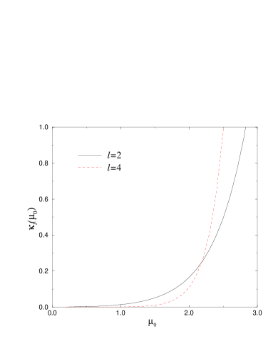
FIG. 9.: The $\kappa_{\ell}$ coefficient as a function of $\mu_{0}$.

If the $\ell=0$ term in the sum for $\Phi$ is explicitly evaluated (note that $\kappa_{0}(\mu_{0})=1/4$) the result is

$$\Phi=\left(1+\frac{M}{2R}\right){\cal F},$$ (40)

with

$${\cal F}\equiv 1+2\left(1+\frac{M}{2R}\right)^{-1}\!\!\sum_{\ell=2,4...}\!\!\kappa_{\ell}(\mu_{0})\left(M/R\right)^{\ell+1}P_{\ell}(\cos\theta).$$ (41)

Since $R$ is analogous to the radial coordinate in isotropic coordinates for a spherical geometry, we introduce a Schwarzschild-like radial coordinate $r$ by the transformation

$$R=\frac{1}{4}\left(\sqrt{r}+\sqrt{r-2M}\right)^{2}$$ (42)

that relates the two coordinates in the Schwarzschild geometry. With this transformation we arrive, finally, at

$$ds^{2}_{\rm Misner}={\cal F}(r,\theta)^{4}\left(\frac{dr^{2}}{1-2M/r}+r^{2}d\Omega^{2}\right)$$ (43)

in which the $r$ and $\theta$ dependence of ${\cal F}$ are given by (41) and (42). It is easy to show that a choice of time coordinate $t$ can be made so that the 4-geometry generated by the Misner initial data takes the form

$$ds^{2}= -\left(1-\frac{2M}{r}\right)dt^{2}$$ (45)

$$+{\cal F}(r,\theta)^{4}\left[\frac{dr^{2}}{1-2M/r}+r^{2}d\Omega^{2}\right]$$

at $t=0$ with all first time derivatives of the metric vanishing.

The function ${\cal F}$ may therefore be thought of as containing the mathematical description of how the Misner geometry initially deviates from the Schwarzschild geometry.

In treating (45) as a distorted Schwarzschild geometry we are taking the range of $r$ to be $2M<r<\infty$ and hence, by (42), our range of coordinates must include all points with $R>M/2$. But according to the transformation in (31) the values of $R$ at $\eta=0$ are limited (by the condition $|\mu|<\mu_{0}$) to values for which

$$R\geq a\coth{\mu_{0}/2}=(M/4\Sigma_{1})\coth{\mu_{0}/2}\quad.$$ (46)

Thus our coordinates can reach down to $R=M/2$, while corresponding to $|\mu|\geq\mu_{0}$ only if $\coth{\mu_{0}/2}\leq 2\Sigma_{1}$, and this condition turns out to be satisfied only for $\mu_{0}\leq 1.191$. We ignore this restriction and find (see below) that the perturbation approach gives reasonably accurate answers for values of $\mu_{0}$ somewhat larger than 1.191. The explanation is that all the strong non-spherical deviations are very close to the horizon and end up not having important consequences for emitted radiation.

Note that the Misner geometry with the $\kappa_{\ell}$ set to zero would be precisely a $t=$ const. slice of the Schwarzschild geometry. The deviations from Schwarzschild are determined by the $\kappa_{\ell}$’s in (41). If they are sufficiently small then the Misner geometry may be considered initially to be a perturbed Schwarzschild geometry. Since the Schwarzschild geometry is stable, sufficiently small initial perturbations will remain perturbations, and the spacetime generated from the Misner initial data will be a perturbed Schwarzschild spacetime. A crucial point is that the form of the initial data interior to the initial horizon cannot affect the evolution of the exterior. We can, therefore, view the generation of outgoing waves — a process confined to the exterior of the horizon — as nearly spherically symmetric if the initial data is nearly spherically symmetric only outside the horizon. More specifically: if $M/R$ is of order unity, or smaller, outside the initial horizon, and if the $\kappa_{\ell}(\mu_{0})$ coefficients are small, then the evolved spacetime outside the horizon will be a perturbed Schwarzschild geometry.

This picture makes sense only if the coefficients ${\kappa}_{\ell}$’s become small when $\mu_{0}\rightarrow 0$, and if this limit corresponds to the “close limit” in which the separation of the two black holes vanishes. To show the former we notice that $(\coth{n\mu_{0}})^{\ell}/\sinh{n\mu_{0}}\approx(n\mu_{0})^{\ell+1}$ for $n\mu_{0}<<1$. We assume that this approximation is valid for small $\mu_{0}$, and we keep terms in summations only up to $N\sim 1/\mu_{0}$. With these approximations we have, for $\ell\geq 1$.

$$\sum_{n=1}^{\infty}\frac{(\coth{n\mu_{0}})^{\ell}}{\sinh{n\mu_{0}}}\approx\frac{1}{({\mu_{0}}^{\ell+1})}\sum_{1}^{N}\frac{1}{n^{\ell+1}}\approx\frac{\zeta(\ell+1)}{{\mu_{0}}^{\ell+1}}$$ (47)

and similarly

$$\Sigma_{1}\equiv\sum_{1}^{\infty}\frac{1}{\sinh{n\mu_{0}}}\approx\frac{1}{\mu_{0}}\sum_{1}^{N}\frac{1}{n}\approx\frac{\ln{N}}{\mu_{0}}\approx\frac{|\ln{\mu_{0}}|}{\mu_{0}}\quad.$$ (48)

These approximations in (39) give us

$$\kappa_{\ell}(\mu_{0})\approx\frac{\zeta(\ell+1)}{|4\ln{\mu_{0}}|^{\ell+1}}\quad.$$ (49)

Although the steps used to derive this result were very rough approximations, the result is in good agreement with numerical values of the $\kappa_{\ell}(\mu_{0})$ s.

We turn now to the question of the separation of the throats in the limit of small $\mu_{0}$. The proper distance $L$ between the throats (more specifically, the distance from $\mu=-\mu_{0}$ to $+\mu_{0}$ along the line $\eta=\pi$) can be written as the sum[26]

$$L=2a\left(1+2\mu_{0}\sum_{1}^{\infty}\frac{n}{\sinh{n\mu_{0}}}\right)\quad.$$ (50)

Here it will be more useful to use an equivalent result in which $L(\mu_{0})$ is given implicitly in terms of $K$ and $E$, the complete elliptic integrals of the first and second kind:

$$L=(4a/\pi)K\left[(1-k^{2})^{1/2}\right]E(k)$$ (51)

$$\mu_{0}=\pi K(k)/K\left[(1-k^{2})^{1/2}\right]\quad.$$ (52)

If $\mu_{0}$ is small, then this forces $k\ll 1$ so that $E(k)\approx K(k)\approx\pi/2$, and

$$L=(\pi^{2}a/\mu_{0})\left[1+{\cal O}(k^{2})\right]$$ (53)

with $k\approx 4\exp{(-\pi^{2}/2\mu_{0})}$. We then have

$$\frac{L}{M}\approx\frac{\pi^{2}}{4\mu_{0}\Sigma_{1}}\approx\frac{\pi^{2}}{4|\ln{\mu_{0}}|}\quad,$$ (54)

and hence the separation decreases as $\mu_{0}$ decreases.

We can then consider $\epsilon\equiv 1/|\ln{\mu_{0}}|$ to be a perturbation parameter, with which we can evolve the Misner initial using perturbation theory. The form of the series in (41) appears to give a multipole decomposition of the deviations from spherical symmetry. This is not quite true. The metric perturbations involve ${\cal F}$ raised to the fourth power. When this is done terms of different multipolarity in ${\cal F}$ mix to give each multipole of ${\cal F}^{4}$. The quadrupole term in ${\cal F}^{4}$, for example, will contain contributions from the product of the $\ell=2$ and $\ell=4$ terms in ${\cal F}$, from the square of the $\ell=2$ term, etc. The total quadrupole term will contain products of the form $\kappa_{2}\kappa_{4},\kappa_{2}^{2},\kappa_{8}\kappa_{2}\kappa_{4}$, and so forth. This complexity causes no difficulty in practice. Of all the contributions to the quadrupole in ${\cal F}^{4}$, that of lowest order is the O($\epsilon^{3}$) term linear in $\kappa_{2}$; the next lowest order contribution ${\cal O}(\epsilon^{6}$) is that from $\kappa_{2}^{2}$. If we are evolving the initial data with the evolution equations of linear perturbation theory for the quadrupole then we must keep only the part of ${\cal F}^{4}$ that is linear in $\kappa_{2}$. It would be inconsistent to keep any higher order terms since we are ignoring the contributions of order ${\cal O}(\epsilon^{6})$ due to the nonlinear evolution of the initial data. A variation of the same argument applies in the case of other multipoles. If we are using the $\ell$-pole linear equations to evolve the $\ell$-pole initial data, we must keep only the term in ${\cal F}^{4}$ that is linear in $\kappa_{\ell}$. All other $\ell$-pole contributions will be higher order in $\epsilon$. Thus if we are only interested, for each $\ell$-pole order, in the terms that can be treated with linearized perturbation theory, we may write ${\cal F}^{4}$ as

$${\cal F}^{4}\approx 1+8\,(1+\frac{M}{2R})^{-1}\!\!\sum_{\ell=2,4...}\kappa_{\ell}(\mu_{0})\left(M/R\right)^{\ell+1}P_{\ell}(\cos\theta),$$ (55)

where

$$P_{\ell}(\cos\theta)=\sqrt{\frac{4\pi}{2\ell+1}}Y_{\ell 0}(\theta,\phi)\quad.$$ (56)

To evolve these even parity perturbations we use the formalism and the notation of Moncrief [16]. From Eqs. (5.1)–(5.8) of that paper, applied to the perturbed spacetime of our Eqs. (45)–(55), we find that Moncrief’s perturbation functions $h_{1}$ and $G$ vanish, and

$$H_{2}=K={\cal G}_{\ell}(r;\mu_{0})=8\sqrt{\frac{4\pi}{2\ell+1}}\kappa_{\ell}(\mu_{0})\frac{(M/R)^{\ell+1}}{1+M/2R}$$ (57)

and Moncrief’s $q_{1}$ is

$$q_{1}= 2r\left(1-\frac{2M}{r}\right)\left[{\cal G}_{\ell}-\sqrt{1-\frac{2M}{r}}\frac{d}{dr}\left(\frac{r{\cal G}_{\ell}}{\sqrt{1-\frac{2M}{r}}}\right)\right]$$ (59)

$$+\ell(\ell+1)r{\cal G}_{\ell}\quad.$$

We then define, for any $\ell$

$$\psi_{\rm pert}\equiv\frac{(\ell+2)(\ell-1)}{(\ell+2)(\ell-1)+6M/r}q_{1}\quad.$$ (60)

For $\ell=2$ note that $\psi_{\rm pert}$ is identical to the $\psi$ of [27]. Note also that the definitions here for the metric perturbations are closely related to those in Eqs.(2)-(4), except that the normalization used for $\psi$ is different (see below).

At this point it should be observed that in Eqs. (57) to (60) the metric perturbations are proportional to $\kappa_{\ell}(\mu_{0})$ and that there is no other $\mu_{0}$ dependence in the perturbations. We may therefore view these expressions, for each $\ell$-pole moment, as first-order perturbation theory in $\kappa_{\ell}(\mu_{0})$. From a formal point of view we may consider that we have a family of spacetimes parameterized by $\mu_{0}$, and we are approximating the metric by

$$g_{\alpha\beta}\approx\left.g_{\alpha\beta}\right|_{\kappa_{\ell}(\mu_{0})=0}+\left.\frac{\partial g_{\alpha\beta}}{\partial\kappa_{\ell}(\mu_{0})}\right|_{\kappa_{\ell}(\mu_{0})=0}\times\kappa_{\ell}(\mu_{0})\ .$$ (61)

It is important to realize that we could just as well do perturbation theory using another expansion parameter $\tilde{\kappa}_{\ell}(\mu_{0})$ that agrees to linear order with $\kappa_{\ell}(\mu_{0})$; we might for example use $\tilde{\kappa}_{\ell}(\mu_{0})=\kappa_{\ell}(\mu_{0})+\left[\kappa_{\ell}(\mu_{0}\right]^{2}$. In terms of this parameter our first-order approximation would be

$$g_{\alpha\beta}\approx\left.g_{\alpha\beta}\right|_{\tilde{\kappa}_{\ell}(\mu_{0})=0}+\left.\frac{\partial g_{\alpha\beta}}{\partial\tilde{\kappa}_{\ell}(\mu_{0})}\right|_{\tilde{\kappa}_{\ell}(\mu_{0})=0}\times\tilde{\kappa}_{\ell}(\mu_{0})$$

$$=\left.g_{\alpha\beta}\right|_{\kappa_{\ell}(\mu_{0})=0}+\left.\frac{\partial g_{\alpha\beta}}{\partial\kappa_{\ell}(\mu_{0})}\right|_{\kappa_{\ell}(\mu_{0})=0}\times\tilde{\kappa}_{\ell}(\mu_{0})$$ (62)

The perturbations here differ from those in (61) by the factor $\tilde{\kappa}_{\ell}(\mu_{0})/\kappa_{\ell}(\mu_{0})$. The approximation given by first-order perturbation theory, then, is dependent on our choice of expansion parameter. This, of course, is a reflection of the fact that first-order perturbation theory must be uncertain to second-order in the expansion factor, but it should be kept in mind that the remarkably good predictions of perturbation theory at unexpectedly large values of $\mu_{0}$ are to some extent due to the particular (though rather natural) use of $\kappa_{\ell}(\mu_{0})$ as the effective expansion parameter.

The function $\psi_{\rm pert}$ is evolved with the Zerilli equation

$$\frac{\partial^{2}\psi_{\rm pert}}{\partial t^{2}}-\frac{\partial^{2}\psi_{\rm pert}}{\partial r^{\ast 2}}-V(r^{\ast})\psi_{\rm pert}=0$$ (63)

in which $r^{\ast}$ is a “tortoise” coordinate such that $r^{\ast}\rightarrow\infty$ corresponds to spatial infinity and $r^{\ast}\rightarrow-\infty$ corresponds to the horizon,

$$r^{\ast}\equiv r+2M\ln{\left(\frac{r}{2M}-1\right)}\quad.$$ (64)

and the Zerilli potential is given by,

$$V(r^{\ast})= \left(1-\frac{2M}{r}\right)\left\{\frac{1}{\lambda^{2}}\left[\frac{9M^{3}}{2r^{5}}-\frac{3M}{r^{3}}\left(1-\frac{3M}{r}\right)\right]\right.$$ (66)

$$\left.+\frac{6}{r^{2}\lambda}\right\}$$

and $\lambda\equiv 1+3M/2r$.

The initial form of $\psi_{\rm pert}$, given by Eqs. (57)-(60), is shown in Fig. 10 along with the potential for the Zerilli equation. Both the and $\ell=2$ and $\ell=4$ figures are shown.

FIG. 10.: We show the initial perturbation waveform, computed at $t=0$ directly from the Misner initial data, and the Zerilli potential for $\ell=2,4$.

It is straightforward to show that, in terms of $\psi_{\rm pert}$, the radiation power is given by

$$\frac{d{\rm Power}}{d\Omega}= \frac{1}{16\pi}\left(\frac{d\psi_{\rm pert}}{dt}\right)^{2}\left[\frac{(\ell-2)!}{(\ell+2)!}\right]^{2}$$ (68)

$$\times\left(\frac{\partial^{2}Y_{\ell 0}}{\partial\theta^{2}}-\cot\theta\frac{\partial Y_{\ell 0}}{\partial\theta}\right)^{2}$$

and therefore,

$${\rm Power}=\frac{1}{16\pi}\left(\frac{d\psi_{\rm pert}}{dt}\right)^{2}\frac{(\ell-2)!}{(\ell+2)!}$$ (69)

Since the waveforms and power depend on $\mu_{0}$ only through factors of $\kappa_{\ell}(\mu_{0})$, we can compute with $\kappa_{\ell}$ set to unity, and get the correct results for any $\mu_{0}$ by multiplying waveforms and power expressions respectively by $\kappa_{\ell}(\mu_{0})$ and $\kappa_{\ell}(\mu_{0})^{2}$.

The above formalism has been used to generate the waveforms and the energies that are presented below and compared to the results of numerical relativity. In the comparisons we must take account of the fact that different normalization conventions than those above have been used to define the wave function $\psi_{\rm num}$. The comparisons will be made by converting the perturbation waveform according to

$$\psi_{\rm num}=\sqrt{2\frac{(\ell-2)!}{(\ell+2)!}}\psi_{\rm pert}$$ (70)

B Comparison of results

Probably the most important comparison to be made is the radiated energy computed by the different methods for dealing with the outgoing radiation. In Fig. 11 this comparison is given. The numerical relativity supercomputer results are shown along with error bars indicating the range of energies found by extracting waveforms at different radii. There are no analogous formal errors for the close-limit or the perturbation-paradigm approach.

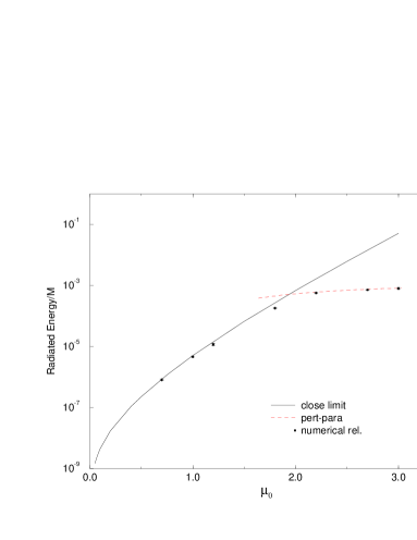
FIG. 11.: Comparison of the close approximation energy with the full numerical results and the particle-membrane approximation

The results show remarkable agreement (already noted in [27]) between the close-limit prediction and the results of fully nonlinear numerical relativity. This agreement is reasonably good even up to $\mu_{0}=2$, where the energy results differ by only 15%. Above $\mu_{0}=2$ the results quickly diverge, with the close-limit results seriously overestimating the radiated energy. For these cases, however, the perturbation-paradigm method gives excellent agreement with computed results (as has already been noted in [5, 6]).

The energies shown in Fig. 11 are strongly dominated by the quadrupole contribution. It is instructive to look at the $\ell=4$ energy predictions of numerical relativity and of the close limit. In the case of the close limit, the $\ell=4$ energy is computed in the manner explained in Sec. IVA. In the numerical relativity results the $\ell=4$ results must be extracted by fitting the angular pattern as explained in Sec. II. The numerical $\ell=4$ results lack the clear trend, seen in Fig. 12, of agreement at small $\mu_{0}$, monotonically growing worse with increasing $\mu_{0}$.

FIG. 12.: Comparison of energies for both the $\ell=2$ and $\ell=4$ modes. The numerical relativity results are denoted by symbols showing the specific case computed, while the close approximation results are denoted by lines.

A better understanding of the sources of disagreement of the method follows from an examination of the “waveforms,” the time dependence of the perturbation function $\psi$ at a constant radius. Figure 13 shows a series of waveforms “observed” at $r=25M$ (where here and below $M$ refers to the ADM mass of the initial data), and show the astonishingly good agreement at small $\mu_{0}$, agreeing in form not only in the region dominated by “ringing” at the quasinormal frequency, but also agreeing at early times. As $\mu_{0}$ increases, the curves continue to agree in general character, but disagree in the amplitude of the quasinormal ringing. Only a single interesting feature (aside from the agreement!) appears in these curves. There is a consistent phase drift between the close-limit waveforms, and the numerical relativity waveforms; the late-time quasinormal ringing of the numerical relativity waveforms has a frequency too low by 10–20%. (The correct values of the quasinormal frequencies are well known from other calculations. See e.g., [28]). As pointed out in Sec. II, this suggests that there is a systematic effect in the present numerical relativity computations causing this phase drift and leading to underestimates of radiated energy. Any increase in the numerical computed energy at large $\mu_{0}$ will, of course, improve the agreement with the close-limit estimates.

FIG. 13.: Comparison of the $\ell=2$ waveforms obtained by the close approximation and those obtained by full numerical relativity for several cases.

The comparison of $\ell=4$ waveforms, at $r=25M$, shown in Fig. 14, clarifies the trends in Fig. 12. For small $\mu_{0}$ numerical errors in the multipole extraction scheme result in waveforms which are clearly in error. Not only do the waveforms lack the expected quasinormal ringing, they have a non-physical trend at late times. These errors are so large simply because at small $\mu_{0}$ the radiation is overwhelmingly dominated by the quadrupole part. At $\mu_{0}=1.0$, for example, the $\ell=4$ contribution is only 1% of the amplitude of the wave. As pointed out in Sec. II, extraction of this very small part is very sensitive to numerical noise. As $\mu_{0}$ increases the relative size of the $\ell=4$ contribution increases, and the numerical error involved in extracting it decreases. For $\mu_{0}\approx 1.2-1.3$ the numerical errors are small enough so that the waveforms show overall reasonable agreement (along with curious features at early and late times). At larger values of $\mu_{0}$ it would be expected that the extracted waveforms would continue to be more accurate, but the lack of a monotonic increase in energy shows that the errors in the waveforms are still very large. Though the large errors make conclusions uncertain, the results suggest that the linearized approach in the close-limit method has a smaller range of validity for $\ell=4$ than for $\ell=2$. Despite this somewhat smaller range of validity the point should not be missed that at the present state of the art in numerical relativity, the close-limit waveforms and energies, for a range of $\mu_{0}$, are the only reliable estimates available for $\ell>2$.

FIG. 14.: Comparison of the waveforms for $\ell=4$ from the close approximation and from numerical relativity.

The waveforms presented above have been “observed” at radius $r=25\,M$. That is, the figures showed $\psi(r=25\,M,t)$. To explore the sensitivity of the comparisons to different observation radii, in Figs. 15 we present $\mu_{0}=1.2$ waveforms observed at different radii. Close-limit waveforms are shown in Fig. 15a, and those of numerical relativity in Fig. 15b.

FIG. 15.: (a,b)Comparison of the waveforms “observed” at different radii for the close approximation and full numerical cases for $\mu_{0}=1.2$. (a) shows the results of the close approximation and (b) shows the full numerical relativity results. The phases have been adjusted for comparison of the waveform shape at the different radii.

In these figures the phases of all waveforms have been made compatible with each other, and with Figs. 13 and 14. Each waveform has been shifted by a time equal to the difference in observation values of $r^{\ast}$, and the value of $r^{\ast}$ equivalent to $r=25\,M$. In Figs. 15 we see that these phase corrected waveforms agree very well at late times, but have somewhat different initial shapes. At early times the waveform observed at smaller radius is larger than if observed at larger radius. This, of course, is a manifestation of the fact that at very early times what we are seeing is essentially the initial data, which – unlike the outgoing radiation – falls off in radius. This effect, the presence of a non-radiative part of the waveform, is significant up to around the first peak of quasinormal ringing. It is important to note that the differences in waveforms observed at different radii are present in both the close-limit and the numerical relativity results. In fact, the differences in the waveforms for different radii are much larger than the differences between the waveforms computed by numerical relativity and by the close-limit approximation.

The waveform comparison to this point has been between the computations of numerical relativity and the close-limit approximation. We now tie this work together with the particle-membrane calculation described in section III B. Although the two approximations are based on different limits, as we have seen they nearly overlap if the two holes are not too far or too close. In Fig. 16 we show results from all three approaches we have used in this paper for the case $\mu_{0}=2.0$. The solid line shows the close approximation, the dashed line shows the results from the full numerical relativity calculation, and the dotted line shows the particle-membrane calculation for the time symmetric particle perturbation. It is important to emphasize that the three graphs shown contain no adjustable parameters.

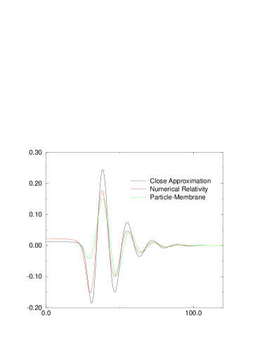
FIG. 16.: Comparison of the waveforms for the particle-membrane approximation, numerical relativity and the close approximation for the case $\mu_{0}=2.0$. These three calculations, containing no adjustable parameters, agree remarkably well, although for this separation the close approximation is near the limit of its applicability.

The waveforms show good agreement at late retarded time, when the behavior is dominated by quasinormal ringing. The waveform computed from the close limit has a higher amplitude, as this approximation is not as accurate for holes at such a large separation parameter. There is, however, a more significant difference in the shape of the early waveforms. Here it is the particle-membrane approach that differs from the other calculations. As discussed in Sec. III B, for this $\mu_{0}=2.0$ case, the extraction of a waveform is difficult and is sensitive to the details of the extraction procedure. Overall, in view of the very different nature of the three calculations, and their different regimes of validity, the agreement among these results is remarkable.

V Discussion and Conclusion

Conventional wisdom holds that events involving colliding black holes are so nonlinear that they can only be studied using numerical relativity. We have shown in this paper that this is not necessarily the case. In particular, we have shown that the head-on collision of two black holes (whose starting point is the Misner initial data) is amenable to semi-analytic treatments giving reliable results in a considerable range of the parameter space.

In the Misner data, the initial separation of the two black holes is determined by the value of the parameter $\mu_{0}$. At present, our numerical techniques are capable of evolving the Misner data, and of extracting waveforms, for the range $0.7\leq\mu_{0}\leq 3.0$, corresponding to initial proper separations $L$ ranging from $1.51M$ to $7.92M$. For $\mu_{0}<1.8$ ($L<3.38M$, corresponding to $r_{0}=2.82M$), the black holes are surrounded by a common event horizon. In such cases the perturbative treatment (“close limit”) described in Sec. IV provides a reliable framework for approximating the true evolution of the spacetime, and the resulting waveforms match nicely those obtained numerically. For $\mu_{0}>1.8$, the black holes are truly distinct, and we find that the waveforms can be well reproduced using the “particle-membrane” treatment described in Sec. III. This approach can also be used to “predict” the waveforms produced during large-$\mu_{0}$ collisions, cases which should be amenable to numerical calculation in the near future.

We note that in Sec. III B and IV B, the comparisons between the numerical and semi-analytic waveforms are made without using a single adjustable parameter. For the $\ell=2$ component of the waveforms (the dominant component), the agreement between the numerical and semi-analytic approaches is remarkable. For $\ell=4$, extraction of the waveforms from the numerical data is less accurate, especially for smaller values of $\mu_{0}$. As a result, and as shown in Sec. IV B, the numerical and semi-analytic $\ell=4$ waveforms differ significantly when $\mu_{0}\leq 1.0$. For larger values of $\mu_{0}$, the $\ell=4$ waveforms agree well in wavelength and in phase, but less so in amplitude. This is illustrated in Figs. 14. To explain this, we note that the waveform amplitude is more sensitive than other waveform attributes (such as wavelength) to the choice of parameters (such as resolution) used in the numerical calculation.

What have we learned about the Misner data through the semi-analytic studies? For gravitational waves observed at large radii, the small $\mu_{0}$ cases of the Misner data actually represent just one single black hole with non-spherical perturbations, although the spacetime in the near field region can be very different. For larger values of $\mu_{0}$, we have seen that the initial data sets represent not just two throats in time symmetric motions. The waves coming from the past null infinity and the past horizon play important roles, namely, they cancel, to a large extent, the radiation emitted before the time symmetric point of the trajectories. We have also seen that the internal dynamics of the black holes do not have much effect on energies or waveforms observed at large radii.

We are currently extending the semi-analytic approaches to other types of black-hole events. We feel that such alternative approaches are an important complement to the direct numerical integration of the Einstein equations. Although these techniques cannot replace numerical relativity, which will be the only means of computing detailed waveforms in more complicated spacetimes such as the full 3D inspiral of two black holes, they can augment it in a number of ways. First, they can be used to test the accuracy of the numerical results, as was illustrated in this paper. Second, they can predict results well in advance of the full-blown numerical treatment. Third, they are inexpensive computationally, and can therefore be used to search the parameter space (initial separation, angular momenta, mass ratio, etc.) for potentially interesting phenomena, to be further investigated using numerical relativity. Fourth, and perhaps most important, alternative approaches help provide a physical understanding of the numerical results.

- [1] A. A. Abramovici, et al., Science 256, 325 (1992).
- [2] L. Smarr, Ph.D. Thesis, University of Texas, Austin, 1975.
- [3] K. Eppley, Ph.D. thesis, Princeton University, 1975.
- [4] L. Smarr, in Sources of Gravitational Radiation, edited by L. Smarr (Cambridge University Press, Cambridge, England, 1979), p. 245.
- [5] P. Anninos, D. Hobill, E. Seidel, L. Smarr, and W.-M. Suen, Phys. Rev. Lett. 71, 2851 (1993).
- [6] P. Anninos, D. Hobill, E. Seidel, L. Smarr, and W.-M. Suen, Phys. Rev. D (1995) (to appear).
- [7] Proceedings of the November, 1994 meeting of the Grand Challenge Alliance to study black hole collisions may be obtained by contacting E. Seidel at NCSA (unpublished).
- [8] P. Anninos, K. Camarda, J. Massó, E. Seidel, W.-M. Suen, and J. Towns, Phys. Rev. D (1995) (in preparation).
- [9] C. Misner, Phys. Rev. 118, 1110 (1960).
- [10] Beware that denotes the total mass in this paper, while in Ref. [6], it is the mass of one hole.
- [11] A. Čadež, Ph.D. thesis, University of North Carolina at Chapel Hill, (1971).
- [12] P. Anninos, D. Bernstein, S. Brandt, D. Hobill, E. Seidel, and L. Smarr, Phys. Rev. D 50, 3801 (1994).
- [13] P. Anninos, D. Hobill, E. Seidel, L. Smarr, and W.-M. Suen, Technical Report No. 24, National Center for Supercomputing Applications.
- [14] A. Abrahams and C. Evans, Phys. Rev. D 42, 2585 (1990).
- [15] A. Abrahams, D. Bernstein, D. Hobill, E. Seidel, and L. Smarr, Phys. Rev. D 45, 3544 (1992).
- [16] V. Moncrief, Annals of Physics 88, 323 (1974).
- [17] M. Davis, R. Ruffini, H. Press, and R. H. Price, Phys. Rev. Lett. 27, 1466 (1971).
- [18] P. Anninos, D. Bernstein, S. Brandt, J. Libson, J. Massó, E. Seidel, L. Smarr, W.-M. Suen, and P. Walker, Phys. Rev. Lett. (1995) (in press).
- [19] S.L. Detweiler and E. Szedenits, Astrophys. J. 231, 211 (1979).
- [20] L. Petrich, S. Shapiro, and I. Wasserman, Astrophys. J. Suppl. Ser. 58, 297 (1985).
- [21] The time symmetry of the event horizon is broken by the definition of the horizon involving the future null infinity but not the past. For further discussion, see R. Matzner, E. Seidel, S. Shapiro, L. Smarr, W.-M. Suen, S. Teukolsky and J. Winicour, submitted to Science.
- [22] S.A. Teukolsky, Astrophys. J. 185, 635 (1973).
- [23] E. Poisson and M. Sasaki, Phys. Rev. D (in press).
- [24] In Black Holes: The Membrane Paradigm, edited by K. S. Thorne, R. H. Price and D. A. Macdonald (Yale University Press, London, 1986), page 284.
- [25] C. W. Misner, Ann. Phys. 24, 102 (1963).
- [26] R. W. Lindquist, Jour. Math. Phys. 4, 938 (1963).
- [27] R. H. Price and J. Pullin, Phys. Rev. Lett. 72, 3297 (1994).
- [28] E. Leaver, Proc. R. Soc.London A402, 285 (1985).