Four Dimensional Quantum Topology Changes of Spacetimes

Abstract

We investigate topology changing processes in the WKB approximation of four dimensional quantum cosmology with a negative cosmological constant. As Riemannian manifolds which describe quantum tunnelings of spacetime we consider constant negative curvature solutions of the Einstein equation i.e. hyperbolic geometries. Using four dimensional polytopes, we can explicitly construct hyperbolic manifolds with topologically non-trivial boundaries which describe topology changes. These instanton-like solutions are constructed out of 8-cell’s, 16-cell’s or 24-cell’s and have several points at infinity called cusps. The hyperbolic manifolds are non-compact because of the cusps but have finite volumes. Then we evaluate topology change amplitudes in the WKB approximation in terms of the volumes of these manifolds. We find that the more complicated are the topology changes, the more likely are suppressed.

I Introduction

In classical gravity the topology change of the universe can be considered only in the case that normally assumed principle like causality is violated[1]. In quantum gravity, on the other hand, topology changing processes are rather ubiquitous. For example, topology changes can happen in the birth of the universe, in the evaporation of a black hole and so on. Moreover, the topology changes, if possible by any mechanism either in classical or quantum gravity, may induce important physical effects.

Recently there have been new progresses in the investigation of topology changes. In (2+1)-dimensional simplified models, the topology changes have been demonstrated to happen indeed by some explicit examples. In three dimensional spacetimes with a negative cosmological constant, two kinds of topology changes have been investigated. The first one was associated with the existence of a compactified three dimensional black hole solution (or a higher genus universe with a negative cosmological constant). One of present authors (M. S.) showed that its analytical continuation around the coordinate singularity of the spacetime may provide a process of topology change[2]. The second one was in the context of quantum cosmology. Fujiwara, Higuchi, Hosoya, Mishima and one of the present authors (M. S.)[3] constructed topology changing solutions by quantum tunneling. To discuss more physical topology changes these works should be generalized to four dimensional spacetimes. The former will be generalized to the (3+1)-dimensional compact hyperbolic cosmology[4]. The purpose of the present article is the generalization of the latter. That is to say, we investigate quantum topology changes in a cosmological model through tunneling processes in four dimensions.

According to Gibbons and Hartle[5], a quantum tunneling spacetime is semi-classically approximated by a Riemannian manifold with totally geodesic boundaries. In Ref.[3], the authors found some constantly curved Riemannian manifolds with topologically non-trivial, totally geodesic boundaries. If such a manifold has two connected pieces of boundary components with different topologies, it describes a process of topology change between the two Lorentzian spacetimes connected on the boundaries. Such 3-manifolds were constructed out of regular truncated polyhedra embedded in a hyperbolic 3-space. In the present article, we discuss the topology change of the universe along the same line but in four dimensions. The four dimensional analogue of polyhedra is called polytope and we shall construct four dimensional Riemannian manifolds by four dimensional regular truncated polytopes embedded in a hyperbolic 4-space[6]. The resultant manifolds describe topology change of a vacuum universe with a negative cosmological constant.

In the next section II we briefly review quantum tunnelings of spacetimes in general, and give a mathematical preliminary for hyperbolic space and quotient manifolds. The section III gives topology changing solutions in four dimensional spacetimes of a constant negative curvature. We investigate their amplitudes and discuss the strong rigidity of the tunneling manifolds in the section IV. The final section V is devoted to summary and discussions.

II Quantum Tunneling of Spacetimes and Hyperbolic Manifolds

A Quantum Tunneling of Spacetimes — formalism

In the context of quantum cosmology, a quantum tunneling should be described by Riemannian path integral formalism proposed by Hartle and Hawking [7]. We would like to appeal to the WKB approximation to compute tunneling amplitudes, since exact computations are almost hopeless in four dimensions. In this case, a quantum tunneling means a transition (classically forbidden) from a spatial hypersurface ${\Sigma}_{i}$ to another spatial hypersurface ${\Sigma}_{f}$. By topology change of spacetime it is meant that ${\Sigma}_{f}$ is topologically different from ${\Sigma}_{i}$. These hypersurfaces may consist of some disconnected components.

Gibbons and Hartle [5] showed that, in the WKB approximation, the tunneling process is described by a Riemannian manifold which has the boundary components $\Sigma_{i}$ and $\Sigma_{f}$. In the ADM-formalism, a spatial hypersurface $\Sigma$ is characterized by a spatial metric $h_{ij}$ and an extrinsic curvature $K_{ij}$ on it. In a semi-classical picture, an ordinary spacetime manifold $M_{L}$ with a Lorentzian signature (Lorentzian manifold) and a quantum tunneling manifold $M_{R}$ with a Euclidean signature (Riemannian manifold) are connected on the hypersurface $\Sigma$ (see Fig.1). The spatial metric $h_{ij}$ can be uniquely defined in the viewpoints of both of regions, because it is independent of the time coordinates. However, the hypersurfaces connecting $M_{L}$ and $M_{R}$ cannot be arbitrarily chosen. Now we work out the condition the connecting hypersurfaces should satisfy. By a lapse function $N$ and a shift vector $N^{i}$, the extrinsic curvature of $\Sigma$ is defined as

$$K_{ij}=-{1\over 2N}\left({\partial h_{ij}\over\partial\tau}-D_{(i}N_{j)}\right),$$ (1)

in the Riemannian manifold, where $\tau$ is the time coordinate in this region, and it is defined as

$$K_{ij}=-{1\over 2N}\left({\partial h_{ij}\over\partial t}-D_{(i}N_{j)}\right),$$ (2)

in the Lorentzian manifold, where $t$ is the time coordinate in this region. In these definitions, $D_{i}$ is the covariant derivative with respect to $h_{ij}$. Since the time $\tau$ in $M_{R}$ is analytically continued to the time $t$ in $M_{L}$ as $\tau=it$ at $\Sigma$, the analytical continuation of geometrical variables, $h_{ij}$ and $K_{ij}$, requires vanishing $K_{ij}$ and $N_{i}$ at $\Sigma$. Hereafter the boundary hypersurfaces with vanishing extrinsic curvature will be called totally geodesic boundaries. Then on the connecting hypersurface, it must be totally geodesic.

For the sake of cosmological interest and simplicity, in the present article, we consider a vacuum spacetime with a cosmological constant. If we further assume vanishing Weyl curvature, the spacetime has a geometry with constant curvature. Thus the Riemannian tunneling manifold $M_{R}$ becomes locally isometric to one of the following cases, $S^{4}$ (4-sphere), $R^{4}$ (4-plane) or $H^{4}$ (4-hyperboloid). In Ref.[5], however, it was proved that if a 4-manifold has two pieces of disconnected boundaries $\Sigma_{i}$ and $\Sigma_{f}$, the spacetime should violate the energy condition at some points. The energy condition states

$$R_{\mu\nu}V^{\mu}V^{\nu}>0$$ (3)

for all vector $V^{\mu}$. Therefore we can exclude $S^{4}$ from our considerations of topology changing manifolds because the curvature of it is positive definite.

From the Gauss-Codazzi equation, the vanishing extrinsic curvature makes $\Sigma_{i}$ and $\Sigma_{f}$ also have constant curvatures (locally isometric to $S^{3},R^{3}$ or $H^{3}$) if the 4-manifold has a constant curvature. To consider topology changes we need variety of the topologies. The Riemannian manifold locally isometric to $R^{4}$ does not satisfy this requirement because the topology of $\Sigma$ is too restricted (see [17]). On the other hand, since the variety of hyperbolic 3-manifolds (Riemannian manifolds locally isometric to $H^{3}$) is very rich, we will consider the Riemannian manifolds which is locally isometric to $H^{4}$. A vacuum spacetime with a negative cosmological constant can just serve our purpose. Then the main question we want to answer in the present article is posed as

Can we construct a hyperbolic 4-manifold with totally geodesic boundaries $\Sigma_{i}$ and $\Sigma_{f}$ which have different topologies?

Mathematically, hyperbolic 4-manifolds are quotient manifolds of a 4-hyperboloid $H^{4}$ by discrete subgroups of its isometry group $SO(4,1)$. The fundamental region of this quotient 4-manifold is a 4-polytope (four dimensional objects bounded by a collection of polyhedra) embedded into $H^{4}$. Intuitively, a quotient manifold means taking some copies of the fundamental regions with their faces identified pairwisely. If we need a 4-manifold with boundaries, some of the 3-faces of the fundamental regions should remain unidentified which form the 3-boundaries of the 4-manifold. Previously, some (2+1)-dimensional analogues of this have been discussed[3]. Although it is more complicated in four dimensions, by similar procedures, we can determine the fundamental region and then the identifications of its 3-faces in hyperbolic geometry [6].

B Hyperbolic Geometry and Klein Model

To give a hyperbolic structure of four dimensional polytopes we embed them into $H^{4}$. In our constructions, we use $n$-dimensional Klein model (projective model)[6] as the model of hyperbolic geometry. The $n$-Klein model is a model on an open $n$-disk

$$D^{n}=\{x^{i}\in R^{n}|x^{i}x_{i}<1\},$$ (4)

in which a metric is

$$ds^{2}={1\over 1-r^{2}}\left({dr^{2}\over 1-r^{2}}+r^{2}d\Omega_{n-1}^{2}\right).$$ (5)

As $r$ goes to $1$, one approaches a sphere at infinity $\partial D^{n}$. This metric gives a constant sectional curvature $-1$ and has a hyperbolic structure. Then this Klein-model is isometric to the spatial hypersurface of the well-known $n$-dimensional open-universe ($k=-1$).

Here we briefly review the important properties of this model. First, it is easy to find that all totally geodesic (extrinsic curvature vanishing) $m(<n)$-hypersurfaces are $m$-planes in this model. Then we can construct totally geodesic boundaries by connecting such $m$-planes. For example, if $m=n-1$, the $m$-planes bound a polytope. We know that each $m$-plane can be identified with another by the isometry $SO(n,1)$ of $H^{n}$. By these identification we shall construct quotient manifolds. A more important property arises when we consider ideal points outside the sphere at infinity $\partial D^{n}$. As depicted in Fig.2, most of ‘parallel’ $(n$$-$$1)$-planes, which do not intersect each other inside the Klein model $D^{n}$ but intersect outside the sphere at infinity $\partial D^{n}$. For our purpose we consider situations in which some $(n$$-$$1)$-planes share only one point ‘$a$’ outside the sphere at infinity. The $(n$$-$$1)$-planes form a pyramid with the vertex ‘$a$’. There ought to exist a special cone which is tangent to the sphere at infinity. There exists an $(n$$-$$1)$-plane which intersects the cone at the tangent points (exemplified in Fig.3). The virtue of the Klein model is that this $(n$$-$$1)$-plane is orthogonal to all of the planes forming the pyramid.

These facts facilitate our procedure of construction of tunneling manifolds. As an example, we show a simple case of a 2-Klein model of $H^{2}$. In Fig.4, two regular triangles are drawn in the 2-Klein model so that each vertex protrudes from $D^{2}$. As mentioned above, we can draw dotted lines which are orthogonal to the edges of the triangle and truncate off the vertices along these dotted lines. We call such a truncation a regular truncation. Gluing the triangles so that the labeled edges match each other, we get a hyperbolic manifold with three $S^{1}$ boundaries. Since the lines composing the boundaries are geodesic and orthogonal to the edges of the regular triangle, the boundaries become smooth totally geodesic $S^{1}$[8].

Finally we should remark upon the relation between the size of an object bounded by planes and the angles between these planes. In the hyperbolic geometry, if we enlarge the size of the object, the angles decrease. When the size approaches zero, the angles become the same values in Euclidean geometry. An angle on the sphere at infinity $\partial D^{n}$ vanishes. We have no well-defined angle outside the sphere at infinity $\partial D^{n}$.

C Four Dimensional Polytopes

First we prepare regular truncated 4-polytopes in the 4-Klein model of hyperbolic 4-space $H^{4}$. Regular 4-polytopes are 5-cell, 8-cell, 16-cell, 24-cell, 120-cell and 600-cell[10]. For example, “5-cell” means that there are five congruent polyhedra which bound the 4-polytope. We shall consider large polytopes in the 4-Klein model in the following sense:

  1)

All the vertices are outside of the sphere at infinity.

  2)

Each edge of polytopes has intersections with the sphere at infinity.

The above conditions guarantee that a single ideal vertex shared by 3-planes which are cells (polyhedra) bounding the polytope can be regularly truncated off. As a generalization of the discussion in the last subsection, to a vertex, there is a unique 3-plane which is perpendicular to the polyhedra bounding the polytope. Also as mentioned in the previous subsection, the dicellular angle (the angle between two adjacent polyhedra in a 4-dimensional space) decreases as the size of the polytope increases in the hyperbolic geometry. To produce a regular and smooth structure after gluing of polytopes, we choose the size of the polytope to make dicellular angles become $2\pi/n$ ($n$ is an integer). Then the size of the polytopes are restricted further to some discrete values. From a geometrical calculation we can find the allowed dicellular angles of the polytopes. The allowed polytopes are shown in the table 1.

The first column gives the names of polytopes and the second column the polyhedra which bound the polytope. Allowed dicellular angles are shown in the third column. The fourth column shows polyhedra produced by regular truncations. The solid angles of these polyhedra at their vertices are in the fifth column. Here it should be noticed that the edges of the polytope are tangent to the sphere at infinity except for the cases of a 24-cell with a dicellular angle $2\pi/5$ and a 600-cell with a dicellular angle $2\pi/3$. Therefore, in most situations, vertices made by the truncation are on the sphere at infinity (This aspect is reflected in the fifth column since the vertices at infinity have vanishing solid angles). In these cases, the truncated polytopes are of course non-compact (exemplified for the case of 8-cell in the next section). Calculating the volume, however, in the next section, we find that their volumes are finite. In the present article, we only consider these non-compact cases. By allowing the points at infinity, the construction of the tunneling manifold becomes much easier. Because a constructed object is required to be a manifold, we should consider completeness of the construction which gives a restriction at every vertex generally. However, in the special cases with vertices on the sphere at infinity, these restrictions do not exist.

In the next section we shall demonstrate some examples of constructions of Riemannian manifolds which describe topology changing processes. One of such Riemannian manifolds is constructed from twelve 8-cell’s which are 4-polytopes bounded by eight congruent hexahedra. The development of such an 8-cell on 3-space is shown in Fig.5. Gluing faces in four dimensions according to the arrows in Fig.5, we get a 4-dimensional polytope bounded by these eight hexahedra, which has sixteen vertices.

III Riemannian Manifolds with Totally Geodesic Boundaries

A Construction from 8-cell

We can adjust the size of the embedded 8-cell so that all the dicellular angles are $\pi/3$. Then we can show that all vertices are located outside the sphere at infinity $\partial D^{4}$. This 8-cell satisfies the two conditions given in the previous section. The edges of the 8-cell are coincidentally tangent to the sphere at infinity. Each hexahedron of the 8-cell is embedded into an induced 3-Klein model (sub-model of the 4-Klein model) as shown in Fig.6. In this three dimensional figure, all vertices are also outside the sphere at infinity $\partial D^{3}$ and all edges are tangent to the sphere.

To get smooth totally geodesic boundary hypersurfaces, we truncate every vertex of the 8-cell in an analogous way as we did in the 2-dimensional example in IIB. Let us pay attention to the four hexahedra having a vertex in common in Fig.5. The property of the Klein model guarantees the existence of a unique 3-hyperplane which is perpendicular to all of the four hexahedra as mentioned in the previous section. In this way we cut out the regions near the sixteen vertices of the 8-cell by these perpendicular 3-hyperplanes to get a regular truncated 8-cell embedded completely in the 4-Klein model. The truncation of 8-cell induces truncation on every hexahedron bounding the 8-cell. The resultant hexahedron is shown in Fig.6. On each hexahedron the truncation of the vertex of the 8-cell makes a triangle with its vertices on the sphere at infinity $\partial D^{3}$. It is noticed that the triangles share vertices with adjacent triangles (for example, the vertex (u) is shared by the two adjacent triangles $\triangle stu$ and $\triangle uvw$ in Fig.6). In this case, any edge of the original hexahedron can be completely truncated off by the two truncations of the two adjacent vertices connected by the edge (see Fig6).

Because four hexahedra share one vertex in an 8-cell (see Fig.7), each 3-boundary of the 8-cell made by the truncation of a vertex is bounded by four triangles. From Fig.7 we see that the 3-boundary is a tetrahedron whose vertices are on the sphere at infinity (To the cases of other 4-polytopes, see the fourth column of the table 1). Since each tetrahedron is orthogonal to the hexahedra in the hyperbolic 4-space, the dihedral angle of the tetrahedron, which equals the dicellular angle of the 8-cell, is $\pi/3$. The volume integration tells us that such tetrahedra have finite volumes [6] though they are non-compact. A single 8-cell includes sixteen vertices and therefore has sixteen tetrahedra as the boundary after regular truncations.

The next step is to find a certain gluing of appropriate number of regular truncated hyperbolic 8-cell’s by identifying the hexahedra, so that the resultant space becomes a smooth manifold and the collection of the tetrahedra produced by regular truncations form smooth 3-boundaries of the manifold. In mathematical language, we want to find a discrete subgroup of the isometry group $SO(4,1)$ so that the quotient space of $H^{4}$ by the discrete subgroup is a manifold. First we would like to try a generalization to four dimensions of what was illustrated in the simple two dimensional example and see whether a manifold can be formed or not. Below is an example of the trial.

We prepare two regular truncated 8-cell’s and put them in the position so that they have a reflection symmetry as depicted in Fig.8. Gluing the hexahedra $X(=1\sim 8)$ and $X^{\prime}(=1^{\prime}\sim 8^{\prime})$ so that all vertices $(a)\sim(p)$ match, we get a 4-space with sixteen boundary components. To make sure smoothness of this 4-space in terms of hyperbolic geometry, it is sufficient to check the smoothness on the boundaries since the dicellular angles of the 8-cell equal the dihedral angles of the tetrahedra on the boundaries. The inside of a truncated hyperbolic 8-cell is smooth and regular. We can nicely glue the two hexahedra in four dimensions because the hexahedra are totally geodesic. Therefore singular structures possibly appear only on the faces, edges and/or vertices of each hexahedron. From Fig.6 we see that the singularity should appear on the boundary tetrahedra if any. The gluing of the hexahedra induces the gluing on the boundary tetrahedra. Fig.7, for example, shows that the gluing of two tetrahedra corresponding to the vertex $(a)$ both in the unprimed and primed 8-cell’s is determined by the identifications of the truncated hexahedra around the vertex $(a)$. Since each unprimed hexahedron is identified with its primed partner, every face of unprimed tetrahedron is glued with its primed partner so that all vertices match. In this configuration, the topology of this space composed of the two tetrahedra is $S^{3}$. Nevertheless we have only $2\pi/3$ turning around each edge of the tetrahedra after gluing, since only two edges of the tetrahedra with the dihedral angle $\pi/3$ are identified into one edge. This means a singularity by the deficit angle $2\pi-2\times\pi/3=4\pi/3$. Therefore we fail to get a smooth manifold by a simple minded generalization of the 2-dimensional example in the previous section.

However there is a way to improve the construction so that we can get a neat manifold, i.e. without a deficit angle. We consider a branched covering space of this singular space. The appropriate branched covering space can be given by a six-fold cover (twelve tetrahedra) of the original singular space. The faces and vertices of the twelve tetrahedra are labeled as Fig.9 ($i=1\sim 6$). The following pairs of the faces of unprimed and primed tetrahedra are glued so that all labeled vertices match.

$$\begin{array}[]{cccc}A_{1}-A^{\prime}_{1}&B_{1}-B^{\prime}_{3}&C_{1}-C^{\prime}_{2}&D_{1}-D^{\prime}_{4}\\ A_{2}-A^{\prime}_{2}&B_{2}-B^{\prime}_{1}&C_{2}-C^{\prime}_{4}&D_{2}-D^{\prime}_{3}\\ A_{3}-A^{\prime}_{3}&B_{3}-B^{\prime}_{2}&C_{3}-C^{\prime}_{5}&D_{3}-D^{\prime}_{6}\\ A_{4}-A^{\prime}_{4}&B_{4}-B^{\prime}_{6}&C_{4}-C^{\prime}_{1}&D_{4}-D^{\prime}_{5}\\ A_{5}-A^{\prime}_{5}&B_{5}-B^{\prime}_{4}&C_{5}-C^{\prime}_{6}&D_{5}-D^{\prime}_{1}\\ A_{6}-A^{\prime}_{6}&B_{6}-B^{\prime}_{5}&C_{6}-C^{\prime}_{3}&D_{6}-D^{\prime}_{2}\end{array}$$ (6)

For instance, $A_{1}$ is matched with $A^{\prime}_{1}$. All the vertices $p_{1},p_{2},p_{3}$ of $A_{1}$ are identified to the vertices $p_{1},p_{2},p_{3}$ of $A^{\prime}_{1}$, respectively.

Fig.10 shows consistency of the gluing around every edge. There are twelve edges in the six-fold covering space after the gluing. There are six dihedral angles which meet at one edge so that there is no deficit angle since each dihedral angle is $\pi/3$.

On the other hand, the vertices of the tetrahedra are on the sphere at infinity $\partial D^{3}$. By the gluing, these vertices are identified into four points at infinity, $p_{1},p_{2},p_{3},p_{4}$. Such points at infinity are called cusps in the hyperbolic geometry. They are not singularities of the manifold but open boundaries at infinity[6]. Topologically a cusp looks like a torus crossing a half-open interval (see Fig.11). The boundary space composed of twelve tetrahedra is a non-compact smooth manifold, which is called $M_{B8}$ in the present paper.

The cusp will not cause any serious physical problem because one cannot observe the infinity of the universe. On the contrary, the existence of such structures at infinity renders the manifold of primary importance. It is a known fact in mathematics that there is a family of almost isometric compact manifolds limiting a cusped manifold[12]. It is expected that the limiting cusped manifold shares common characters of the family. Furthermore the cusped manifold is the simplest one among the family in some sense. Hence, admitting the cusp to our manifold, we get the following simplest example of topology changing of spacetime by quantum tunneling.

Now we expect that the branched covering proceeded above can be straightforwardly extended to the whole of 8-cell’s. Since the six-fold cover of the boundary 3-space produced by the simple minded identification is the smooth 3-manifold $M_{B8}$, the six-fold cover of the 4-space produced by the simple minded identification will have smooth boundary manifolds, $M_{B8}$’s. We prepare six pairs of unprimed and primed 8-cell’s as Fig.8 (the pairs are labeled by $i=1\sim 6$). Every vertex and cell (hexahedron) of the 8-cell’s are also labeled in Fig.8. All subsequent gluings will be done so that these labeled vertices are matched. We determine the gluing of hexahedra around each vertex $(a)$ of 8-cell’s (cell $1_{i}\sim$ cell $4_{i}$, so that they induce gluing (6) on a tetrahedron made by the truncation of the vertex $(a)$ to form $M_{B8}$. Fig.7 shows the tetrahedron by the truncation of each vertex $(a)$. In this figure, each face of a tetrahedron is labeled by an index of the cell which the face belongs to, and each vertex of the tetrahedron is labeled by the same character as that of the nearest vertex of the hexahedron. From Fig.7 and 9 we find a correspondence, $1_{i}\equiv A_{i},\ 4_{i}\equiv B_{i},\ 3_{i}\equiv C_{i},\ 2_{i}\equiv D_{i}$. By (6), the gluing of the hexahedra, which constructs $M_{B8}$ from the tetrahedra produced by the truncation of the vertex $(a)$ are the following:

$$\begin{array}[]{cccc}1_{1}-1^{\prime}_{1}&4_{1}-4^{\prime}_{3}&3_{1}-3^{\prime}_{2}&2_{1}-2^{\prime}_{4}\\ 1_{2}-1^{\prime}_{2}&4_{2}-4^{\prime}_{1}&3_{2}-3^{\prime}_{4}&2_{2}-2^{\prime}_{3}\\ 1_{3}-1^{\prime}_{3}&4_{3}-4^{\prime}_{2}&3_{3}-3^{\prime}_{5}&2_{3}-2^{\prime}_{6}\\ 1_{4}-1^{\prime}_{4}&4_{4}-4^{\prime}_{6}&3_{4}-3^{\prime}_{1}&2_{4}-2^{\prime}_{5}\\ 1_{5}-1^{\prime}_{5}&4_{5}-4^{\prime}_{4}&3_{5}-3^{\prime}_{6}&2_{5}-2^{\prime}_{1}\\ 1_{6}-1^{\prime}_{6}&4_{6}-4^{\prime}_{5}&3_{6}-3^{\prime}_{3}&2_{6}-2^{\prime}_{2}\ \ .\\ \end{array}$$ (7)

It is a non-trivial problem to determine whether it is possible or not for the tetrahedra produced by the truncations of the other vertices $(b)\sim(p)$ to form $M_{B8}$’s by appropriate choices of gluing of the other cells (cell $5\sim$ cell $8$). Determining the other gluings as shown below, we can see that two adjacent tetrahedra, e.g. formed by the truncations of vertices $(a)$ and $(b)$ (see Fig.12), are symmetric under the inversion because of the symmetry of the 8-cell.

$$\begin{array}[]{cccc}5_{1}-5^{\prime}_{1}&8_{1}-8^{\prime}_{3}&7_{1}-7^{\prime}_{2}&6_{1}-6^{\prime}_{4}\\ 5_{2}-5^{\prime}_{2}&8_{2}-8^{\prime}_{1}&7_{2}-7^{\prime}_{4}&6_{2}-6^{\prime}_{3}\\ 5_{3}-5^{\prime}_{3}&8_{3}-8^{\prime}_{2}&7_{3}-7^{\prime}_{5}&6_{3}-6^{\prime}_{6}\\ 5_{4}-5^{\prime}_{4}&8_{4}-8^{\prime}_{6}&7_{4}-7^{\prime}_{1}&6_{4}-6^{\prime}_{5}\\ 5_{5}-5^{\prime}_{5}&8_{5}-8^{\prime}_{4}&7_{5}-7^{\prime}_{6}&6_{5}-6^{\prime}_{1}\\ 5_{6}-5^{\prime}_{6}&8_{6}-8^{\prime}_{5}&7_{6}-7^{\prime}_{3}&6_{6}-6^{\prime}_{2}\end{array}\ .$$ (8)

Since the inversion of one $M_{B8}$ gives another $M_{B8}$, each group of twelve tetrahedra forms one $M_{B8}$ at each vertex $(b)\sim(p)$. Therefore the glued twelve 8-cell’s have sixteen $M_{B8}$’s on their boundary. Here a fact should be noticed that the tetrahedra are orthogonal to the cells (hexahedra) of the 8-cell, which guarantees that the $M_{B8}$ is smooth at the points at which the tetrahedra join. Then $M_{B8}$ on the boundary is a totally geodesic smooth manifold in $H^{4}$.

Of course these identifications are orientation preserving isometry transformation because of the reflection symmetry between the unprimed and primed 8-cell’s. The resultant space is orientable.

To check that this 4-space is a complete smooth 4-manifold, we consider the neighborhood of the faces, edges and vertices. In four dimensions, when we turn around each face completely, the total angle should be $2\pi$ for consistency. We shall check this consistency on the boundary of it. On the boundary 3-hypersurface, we should check whether it is $2\pi$ or not around the edges ($\alpha,\beta,\gamma...$ in Fig.6) of the tetrahedra. This consistency is guaranteed by our previous analysis where we have shown that the boundary consists of several pieces of the manifolds $M_{B8}$ (see Fig.10). The remaining vertices after the regular truncation ($s,t,u...$ in Fig.6) cause no problem since they form 4-cusps at infinity. Hence this space is a complete smooth non-compact hyperbolic 4-manifold with totally geodesic 3-boundaries. The boundaries are sixteen $M_{B8}$’s.

B Other Solutions

As shown previously in the table 1, there are seven kinds of 4-polytopes admitting regular truncations. Geometrical calculations reveal that two of them, 24-cell with a dicellular angle $2\pi/5$ and 600-cell with a dicellular angle $2\pi/3$, are compact and the others are non-compact after regular truncations. We can apply our method for the twelve non-compact 8-cell’s to these non-compact cases. By a similar method, we can successfully get complete smooth hyperbolic 4-manifolds with totally geodesic 3-boundaries in the two cases. One of them is the case of a 16-cell (bounded by sixteen tetrahedra) with a dicellular angle $\pi/2$ and the other is the case of a 24-cell (bounded by twenty-four octahedra) with a dicellular angle $\pi/3$. Four 16-cell’s form a manifold whose 3-boundaries are eight $M_{B16}$’s (we consider a two-fold cover of a simple minded identifications), where an $M_{B16}$ with six cusps is composed of four octahedra. Similarly, six 24-cell’s also constitute a manifold whose 3-boundaries are twenty-four $M_{B24}$’s (we consider a three-fold cover of a simple minded identifications), where an $M_{B24}$ with eight cusps is composed of six hexahedra.

Here we would like to point out a peculiarity of the hyperbolic manifold by referring to a mathematical fact. For three or four dimensional hyperbolic manifold $M_{3,4}$, the fundamental group $\pi_{1}(M_{3,4})$ determines $M_{3,4}$ uniquely up to an isometry and a choice of normalizing constants[15]. This has been known as the Mostow rigidity. Then it is sometimes sufficient to determine the homology group $H_{1}$ of the hyperbolic manifold in order to distinguish the manifolds, where $H_{1}$ is an Abelian group such that $H_{1}=\pi_{1}/[\pi_{1},\pi_{1}]$. To characterize the boundaries topologically we calculate the corresponding homology groups [16],

$$H_{1}(M_{B8}) = Z+Z+Z+Z;$$ (9)

$$H_{1}(M_{B16}) = Z+Z+Z+Z+Z+Z;$$ (10)

$$H_{1}(M_{B24}) = Z+Z+Z+Z+Z+Z+Z+Z.$$ (11)

Clearly they are topologically inequivalent. Since the rank of the free finite Abelian group part of $H_{1}$ counts the number of two dimensional holes [16], $M_{Bn}$ has a more complicated topological structure than $M_{Bm}$ has if $n>m$. On the other hand, the torsion-free property may be considered as a pleasant feature of the universe because otherwise the universe might be non-orientable. If we had a method which can produce a solution whose boundaries have torsion part, much more solutions could be found.

Incidentally, it is impossible to construct a solution from 5-cell’s or 120-cell’s in our way. The remaining regular truncated polytopes are compact. In the compact case, we should check consistency also around the vertices of the regular truncated polytopes. However it is too complicated for us to work out this consistency check and we need more advanced techniques. This is our project in future [13].

IV Topology Changing Amplitude and Strong Rigidity

We have constructed three hyperbolic 4-manifolds with totally geodesic boundaries. From Gibbons and Hartle[5]; Fujiwara, Higuchi, Hosoya, Mishima and one of the present authors(M. S.) [3], these manifolds can be regarded as instantons causing topology changes by quantum tunneling. For example, the manifold of twelve 8-cell’s can describe the topology changes: ‘from nothing to sixteen $M_{B8}$’s’, ‘from one $M_{B8}$ to fifteen $M_{B8}$’s’ or ‘from two $M_{B8}$’s to fourteen $M_{B8}$’s’, and so on (see Fig.13). It is also worthy of notice that by plumbing them we can get infinite series of topology changing solutions as exemplified in Fig.13. Since each boundary is totally geodesic, the gluing is perfect to make a neat manifold when we identify two boundary components of the same shape and size.

We have demonstrated topology changing processes between non-trivial spatial topologies in four dimensions by quantum tunneling, which cannot be reduced to a lower dimensional subspace. Brill constructed a 4-dimensional topology changing solution which, in fact, is effectively a direct product of a topology changing two dimensional spacetime and the other two dimensional space[8]. Of course, the pair creation of charged black holes[9], in an extended sense, is also a process of topology change. The Riemannian manifold for that process has a single totally geodesic 3-boundary which can be interpreted as a topology change from “nothing” to the space containing a pair of black holes. However, the present paper gives descriptions of processes which include not only the creation of the universe from “nothing” but also the change from $n$ $M_{B}$ to $m$ $M_{B}$ ($n\neq m$). Both of initial and final spatial hypersurfaces ($\Sigma_{i}$ and $\Sigma_{f}$) have non-trivial topologies.

Now let us evaluate the tunneling amplitude for these topology changes. In the context of the Hawking’s Riemannian path integral, the amplitude can be formally described as

$$T(h_{i},h_{f})=\sum_{M_{R}}\int{\cal D}g\exp(-S_{E}[g]),$$ (12)

where $h_{i}$ and $h_{f}$ are the 3-dimensional metrics on the initial and final spatial hypersurfaces $\Sigma_{i}$ and $\Sigma_{f}$, respectively. $S_{E}$ is the Euclidean action,

$$S_{E}=-{1\over 16\pi G}\int_{M_{R}}(R-2\Lambda)\sqrt{g}d^{4}x+{1\over 8\pi G}\int_{\partial M_{R}}K\sqrt{h}d^{3}x\ \ .$$ (13)

The path integral is over smooth 4-metric $g$ on the Riemannian manifold $M_{R}$ which has appropriate boundaries $\Sigma_{i}$ and $\Sigma_{f}$ by assumption. In our cases, $M_{R}$ is one of the 4-manifolds which have been constructed in the previous section. Then we can evaluate the path integral (12) in the WKB approximation for the topology changing processes. The second term comes from the contribution of the boundaries other than $\Sigma_{i,f}$ namely that of the open boundaries at the cusps. It is easy to see by explicit calculation that $K$ vanishes at the cusps. Since our solution has a constant negative curvature $R=4\Lambda<0$, the classical action $\bar{S}_{E}$ is proportional to the 4-volume of the spacetime and is given by

$$\bar{S}_{E}={1\over 8\pi G}{V\over|\Lambda|},$$ (14)

where $V$ is a numerical value of the volume of $M_{R}$ in the case of $\Lambda=-3$. It follows from (14) that the WKB approximation of the tunneling amplitude is exponentially suppressed for a tunneling manifold of a large volume. Then we intuitively expect that the topology change between more complicated topologies requires a larger volume of tunneling manifold and is more suppressed provided that the WKB prefactors are of the same order.

Though our manifolds have cusps, their volumes are finite. Following Kellerhals [14], the hyperbolic volumes of the 4-polytopes that we have used are calculated as

$${\rm Volume(truncated\ 8-cell^{\prime}s)} = {4\pi^{2}\over 3}$$ (15)

$${\rm Volume(truncated\ 16-cell^{\prime}s)} = {4\pi^{2}\over 3}$$ (16)

$${\rm Volume(truncated\ 24-cell^{\prime}s)} = {20\pi^{2}\over 3}$$ (17)

and the volume of the manifolds are summarized in table 2.

The volume of a constant curvature space is given by the Gauss-Bonnet theorem[11],

$$\chi(M)={1\over 32\pi^{2}}\int_{M}\epsilon_{abcd}{\cal R}^{ab}\wedge{\cal R}^{cd}-{1\over 32\pi^{2}}\int_{\partial M}\epsilon_{abcd}(2\theta^{ab}\wedge{\cal R}^{cd}-\frac{4}{3}\theta^{ab}\wedge\theta^{c}_{e}\wedge\theta^{ed}),$$ (18)

where ${\cal R}^{ab}$ and $\theta^{ab}$ are the curvature 2-form and the second fundamental form. Since the boundary $\partial M$ is totally geodesic, $\theta^{ab}$ vanishes there. The Euler numbers $\chi(M)$ are combinatorially determined as

$$\chi({tunneling\ manifold\ consisting\ of\ twelve\ 8-cell^{\prime}s}) = 12,$$ (19)

$$\chi({tunneling\ manifold\ consisting\ of\ four\ 16-cell^{\prime}s}) = 4,$$ (20)

$$\chi({tunneling\ manifold\ consisting\ of\ six\ 24-cell^{\prime}s}) = 30,$$ (21)

and agree with (18) and the volumes given in table 2.

Roughly speaking, more polytopes are needed to get a manifold with a more complicated topological structure. Then we expect that the volumes are largely related to the topological structure (just the Euler number in a constant curvature space). The larger volume will imply a more complicated topological structure. Now let us recall one of the peculiarities of the hyperbolic manifold, Mostow rigidity. For three or four dimensional hyperbolic manifold $M_{3,4}$, the fundamental group $\pi_{1}(M_{3,4})$ determines $M_{3,4}$ uniquely up to an isometry and a choice of normalizing constant[15]. Therefore, our tunneling manifolds include no degrees of freedom of deformation[17] as long as the manifold is hyperbolic. If we include non-zero Weyl curvature, the manifold can become inhomogeneous and the degrees of freedom of deformation becomes dynamical. In such a situation, the quantum theory of the dynamical degrees of freedom have to be developed for a quantum topology change theory.

V Summary and Discussions

In the present paper, we have found instantons which describe topology changing processes by quantum tunneling of spatial hypersurfaces of spacetimes which are locally anti-de Sitter. Here we summarize our results in the table 2.

It may be intuitively expected that the more complicated is the topology of the universe which topologically changes, the larger is the volume of the tunneling manifold. Let us investigate whether this is the case in our examples. From table 2, however, we cannot easily draw a conclusion directly since the number of boundary manifolds are different. Quantitatively, we can compare a set of three topology changing manifolds with $16\times M_{B8}$, a set of six topology changing manifolds with $8\times M_{B16}$ and a set of two topology changing manifolds with $24\times M_{B24}$. All the sets have 48 boundaries though they are not arcwise connected. Then the corresponding manifolds have volumes $48\pi^{2}$, $32\pi^{2}$ and $80\pi^{2}$, respectively. The result is not just what we expected. Although the third one is much larger than the other two, which means that $M_{B24}$ is more unlikely to appear comparing to the other two, the first one and the second one are comparable. What is more, the probability for the first one to appear is smaller than that for the second one. Since $H_{1}(\Sigma)$ characterizes the topological structure of $\Sigma$ by the equations (9), (10) and (11), the boundary of the first one is simpler than that of the second one. However, their volumes imply that the topology of the first one is more complicated than the topology of the second one. Nevertheless, we cannot conclude that the tunneling of $M_{B16}$ has the maximum of probability. There might be a smaller manifold describing the topology change of $M_{B8}$’s. If we could find the relation between the volume of the solution (the Euler number) and the boundary of it, the relation would explain this.

One might think that our constructions are too restricted. First, the identification is determined so as to preserve the symmetry of the polytope. Second, the resultant polytopes are identical with each other. From these restrictions, for example, one cannot consistently identify the polyhedra which bound a single polytope. Our restrictions made the construction simple. However, it may well be the case that there are much more solutions which have been ruled out by the restrictions. To complete the discussion about the topology change by quantum tunneling, we should relax these restrictions. Then the structure of the tunneling manifold becomes more involved. Constructing such complicated cases will need the aid of computer.

When we evaluate the topology changing amplitude, the formalism of Hartle and Hawking has been used. However, the exact no-boundary condition in the original formalism of Hartle and Hawking does not allow the existence of boundary at infinity. In our solutions, the tunneling manifolds have cusped boundaries at infinity. Since the cusped boundaries are infinitely small and the manifolds have finite volumes, we may generalize the formalism of Hartle and Hawking to such a case. If we stick to impose the no-boundary condition in a strict sense, we need compact tunneling manifolds. An investigation in this direction is also in progress[13].

People might be disturbed by the existence of the cusps. If we study the effect of “matter fields” or fluctuations of the metric (“one-loop corrections”), the boundary conditions at the cusps are needed. The conditions and the effects will be studied in appropriately simplified situation[19]. Furthermore, some people might insist that the cusps do not allows one to use Einstein-Hilbert action and the idea of a smooth manifold in this arbitrary small scale. A calculation in the (2+1)-dimensional gravity will reveal something about this as a simplified case. On the other hand, it observationally causes no problem since the cusps are at infinity and we cannot “see” them. We see only the pattern of spatial periodicity[18]. If we observe the pattern of the spatial periodicity as the super large scale structure of the universe, we may be able to determine the topology of our universe and to know whether the universe has the cusps or not.

In the case of the topology change in (2+1)-dimensional quantum tunneling, the rigidity of the hyperbolic manifold is easier to understand. While hyperbolic 2-boundaries have moduli parameters as the dynamical degrees of freedom, the tunneling manifolds do not allow any deformation corresponding to them, which is consistent with the rigidity. In four dimensional case, however, the situation is different because the 3-boundary is also rigid as well as the tunneling manifold itself. The dynamical degrees of freedom will appear only when we allow non-zero Weyl curvature. In such a case the gravitational degrees of freedom should be considered. As a first step we can consider the linear perturbation of them. If we quantize these degrees of freedom, we expect particles be created. This might cause a quantum instability of topology changing solutions if the backreaction to the spacetime is too large.

Acknowledgments

We would like to thank Prof. S. Kojima, Prof. M. Sasaki and Dr. Higuchi for helpful discussions. One of the authors (M. S.) thanks the Japan Society for the Promotion of Science for financial support. This work was supported in part by the Japanese Grant-in-Aid for Scientific Research Fund of the Ministry of Education, Science and Culture.

FIG. 1.: A manifold with a Euclidean signature $M_{R}$ interpolates the two manifolds with a Lorentz signature $M_{L}$ through $\Sigma_{i,f}$

FIG. 2.: A two dimensional example. There are some lines not intersecting each other inside the Klein model $D^{n}$. They are parallel lines and intersect outside the sphere at infinity $\partial D^{n}$.

FIG. 3.: Three planes share the point ‘$a$’ outside the sphere. The cone with the vertex ‘$a$’, is tangent to the sphere at infinity. Then the plane through the tangent points is perpendicular to the three planes.

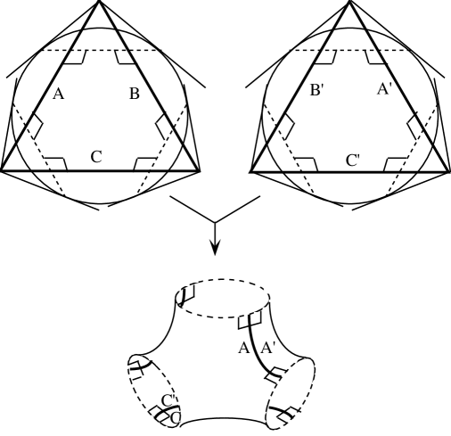
FIG. 4.: Two hexagons made by regular truncations of triangles are glued. The resultant space is one of the simplest topology changing manifolds.

FIG. 5.: The development of an 8-cell. Gluing the faces of the hexahedra along the arrows in four dimensions, we get the 8-cell of a 4-dimensional polytope.

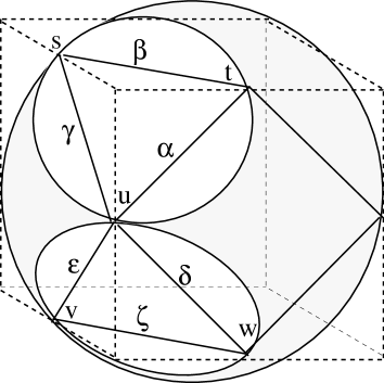
FIG. 6.: The shaded sphere is a sphere at infinity in the 3-Klein model. Each edge of the hexahedra is tangent to the sphere at $s,t,u...$. The sphere is cut by planes through $s,t,u...$. Along these planes we truncate the vertices of the hexahedron.

FIG. 7.: A part of the 8-cell in Fig.5. Four hexahedra meet at a vertex. When we truncate the vertex, a tetrahedron appears. We label the faces and the vertices of the tetrahedra at the vertices $(a)$ by the index number of the cell which the face belongs to and the vertices of the 8-cell’s on the opposite side of $(a)$, respectively.

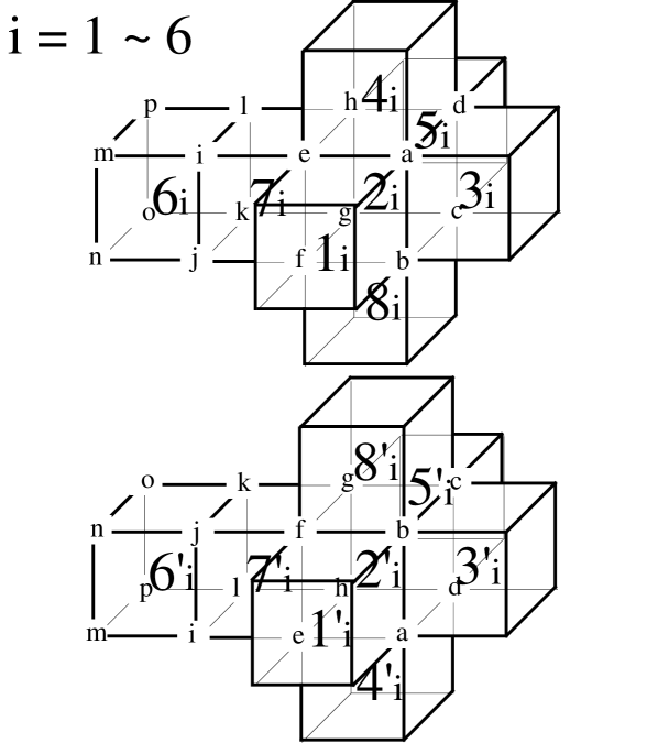
FIG. 8.: Two types of 8-cell’s. Upper ones are left-handed while lower ones (with primes) are right-handed. The corresponding cells with the same number which are primed and unprimed are identified (for example, $1_{1}$ and $1^{\prime}_{1}$, $4_{1}$ and $4_{3}^{\prime}$ …).

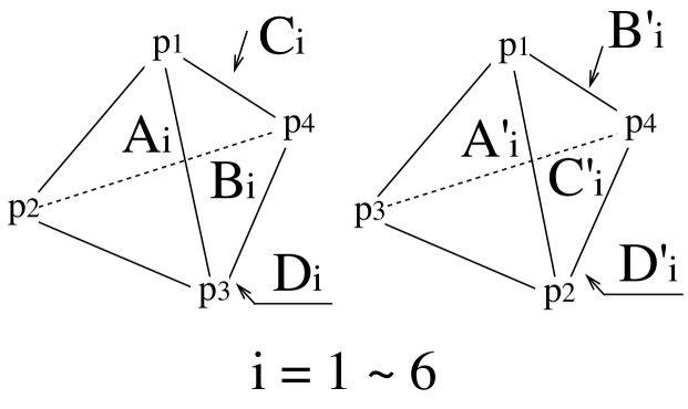
FIG. 9.: Six unprimed tetrahedra and six primed tetrahedra. Twelve tetrahedra constitute $M_{B}8$.

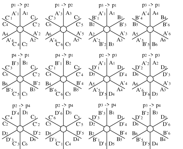
FIG. 10.: The consistency check of the manifold which is composed of the tetrahedra in Fig.9 with the rule of the equation (6). Six dihedral angles meet at the edges in Fig.9. Since each dihedral angle is $\pi/3$, there is no deficit angle.

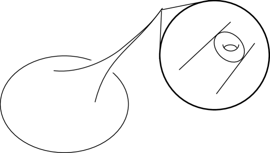
FIG. 11.: An intuitive picture of a cusped hyperbolic manifold. The cusp topologically looks like a torus cross a half-open interval.

FIG. 12.: If we treat $8_{i}$ as if it were $4_{i}$, a tetrahedron from vertex $(a)$ and a tetrahedron from vertex $(b)$ would be symmetric under the inversion.

FIG. 13.: A Riemannian manifold with sixteen boundaries is regarded as a topology change solution ‘from nothing to sixteen $M_{B8}$’s’, ‘from one $M_{B8}$ to fifteen $M_{B8}$’s’ or ‘from two $M_{B8}$’s to fourteen $M_{B8}$’s’, and so on. Furthermore, by plumbing of the solution we can obtain various types of topology change solutions.

polytope bounding dicellular polyhedra made solid angle polyhedra angle by truncation around the vertices 5-cell five tetrahedra $\pi/3$ five tetrahedra 0 8-cell eight hexahedra $\pi/3$ sixteen tetrahedra 0 16-cell sixteen tetrahedra $\pi/2$ eight octahedra 0 24-cell twenty-four octahedra $2\pi/5$ twenty-four hexahedra $4\pi/20$ twenty-four octahedra $\pi/3$ twenty-four hexahedra 0 120-cell 120 dodecahedra $\pi/3$ 600 tetrahedra 0 600-cell 600 tetrahedra $2\pi/3$ 120 icosahedra $4\pi/12$

Table 1

The first column is the name of polytopes, which are bounded by the polyhedra on the second column. The third column gives possible dicellular angles. After regular truncation, there appear new polyhedra shown in the fourth column whose vertices have a solid angle on the fifth column.

building block boundary $\Sigma_{i,f}$ $H_{1}(\Sigma)$ the volume of solutions 8-cell$\times 12$ $16\times M_{B8}$ Z+Z+Z+Z $12\times 6.8009491$ 16-cell$\times 4$ $8\times M_{B16}$ Z+Z+Z+Z+Z+Z $4\times 8.7730176$ 24-cell$\times 6$ $24\times M_{B24}$ Z+Z+Z+Z+Z+Z+Z+Z $6\times 59.2029$

Table 2

The topology changing manifolds that we have constructed. The first column is the polytope we have used. The resultant manifolds have the boundaries on the second column whose homology group $H_{1}$ are shown in the third column. The volume of solutions are displayed on the fourth column.

REFERENCES

- [1] R. P. .Geroch, J. Math. Phys. 8 (1967) 782, P. Yodzis, Gen. Rel. Grav. 4 (1973) 299, D. Gannon, J. Math. Phys. 16 (1975) 2364, F. J. Tipler, Ann. Phys. 108 (1977) 1, R. D. Sorkin, Phys. Rev. D33 (1986) 978.
- [2] M. Siino, Class. Quantum Grav. 11 (1994) 1995.
- [3] Y. Fujiwara, S. Higuchi, A. Hosoya, T. Mishima and M. Siino, Phys. Rev. D44 (1991) 1756, Phys. Rev. D44 (1991) 1763, Class. Quantum Grav. 7 (1992) 163.
- [4] A. Ishibashi, T. Koike, M. Siino, in preparation.
- [5] G. W. Gibbons and J. B. Hartle, Phys. Rev. D42 (1990) 2458.
- [6] W. P. Thurston, The Geometry and Topology of 3-manifold, to be published by Princeton University Press, 1978/79.
- [7] J. B. Hartle and S. Hawking, Phys. Rev. D28 (1983) 2960.
- [8] D. Brill Euclidean Maxwell-Einstein Theory, to appear in Luis Witten Festschrift (World Scientific), gr-qc/9209009.
- [9] D. Garfinkle and A. Strominger, Phys. Lett. 256B (1991) 146; D. Garfinkle, G. Horowitz and A. Strominger, Phys. Rev. D43 (1991) 3140; F. Dowker J. P. Gauntlett, D. A. Kastor and J. Traschen, Phys. Rev. D49 (1994) 2909; D. Garfinkle, S. B. Giddings and A. Strominger, Phys. Rev. D49 (1994) 958; F. Dowker, J. P. Gauntlett, S. B. Giddings and G. T. Horowitz, Phys. Rev. D50 (1995) 2662.
- [10] H. S. M. Coxeter, Regular Polytopes, New York, Dover Publications, 1973.
- [11] T. Eguchi, P. B. Gilkey, and A. J. Hanson, Phys. Rep.66 (1980) 213.
- [12] Private communication with J. Weeks in e-mail.
- [13] M. Siino, in preparation.
- [14] R. Kellerhals, Math. Z.206 (1991) 193.
- [15] G. D. Mostow, Strong Rigidity of Locally Symmetric Spaces, Annals of Mathematics Studies, Princeton, Princeton University Press, 1973.
- [16] C. Nash and S. Sen, Topology and geometry for physicists, London, Academic Press, 1983.
- [17] T. Koike, A. Hosoya and M. Tanimoto J. Math. Phys. 35 (1994) 4855.
- [18] L. Z. Fang and H. Sato, Gen. Rel. Grav.17 (1985) 1117.
- [19] M. Siino, gr-qc/9601001, KUNS 1375.