UCD-95-6

February 1995

gr-qc/9503024

Lectures on (2+1)-Dimensional Gravity
S. Carlip
Department of Physics
University of California
Davis, CA 95616
USA

Abstract

These lectures briefly review our current understanding of classical and quantum gravity in three spacetime dimensions, concentrating on the quantum mechanics of closed universes and the (2+1)-dimensional black hole. Three formulations of the classical theory and three approaches to quantization are discussed in some detail, and a number of other approaches are summarized. An extensive, although by no means complete, list of references is included. (Lectures given at the First Seoul Workshop on Gravity and Cosmology, February 24-25, 1995.)

1. Introduction

General relativity is a notoriously difficult theory. At the classical level, such fundamental issues as cosmic censorship, the nature of singularities, and the conditions for formation of closed timelike curves remain unresolved. At the quantum level, the situation is even worse: despite some sixty years of research, we cannot yet say with any confidence that we understand the basic conceptual foundations of quantum gravity.

Faced with such difficulties, it is natural to look for simpler models that share important features with general relativity. The choice of model depends on what questions one wishes to ask, but for many purposes—especially in the realm of quantum gravity—a particularly useful model is general relativity in three spacetime dimensions. Work on (2+1)-dimensional gravity dates back at least to 1963 [1], and occasional articles appeared over the next twenty years[2, 3, 4]. But credit for the recent growth of interest should probably go to two groups: Deser, Jackiw, and ’t Hooft [5, 6, 7], who examined the classical and quantum dynamics of point sources, and Witten [8, 9, 10], who rediscovered and explored the representation of (2+1)-dimensional gravity as a Chern-Simons theory.

Hundreds of papers about (2+1)-dimensional gravity have appeared since the pioneering work of the mid-1980’s, and the subject has become far too extensive for me to summarize fairly in these lectures. I have therefore chosen to focus on a few key aspects: classical gravity for empty, spatially compact universes, a few approaches to the quantization of this classical physics (“(2+1)-dimensional quantum cosmology”), and the classical and quantum mechanics of the (2+1)-dimensional black hole. I am necessarily leaving out many interesting topics: classical point sources and closed timelike curves (see, for instance, [12, 13, 14, 15]); the classical and quantum behavior of point particles (for a partial sample of extensive work, see [5, 6, 7, 16, 17, 18, 19, 20, 21, 22, 23, 24, 25]); matter couplings (see, for instance, [26, 27, 28, 29, 30, 31]); supergravity (see, for instance, [11, 32, 33, 34, 35]; asymptotic behavior and global “charges” [36, 37, 38]; the radial gauge [39, 40]; topologically massive gravity [41, 42, 43]; Poincaré gauge theory [44, 45, 46]; the construction of observables from topological field theories [47, 48]; and an assortment of other subjects.

The structure of these lectures is as follows. In the next section, I discuss the field equations of classical general relativity in 2+1 dimensions, and obtain the set of solutions for spacetimes with the topology ${\hbox{{\rm I}\kern-1.99997pt\hbox{\rm R}}}\!\times\!\Sigma$, where $\Sigma$ is a closed surface of genus $g\!>\!0$. I summarize three classically equivalent descriptions of these solutions, in terms of gluing patterns of geometric structures, gauge field holonomies arising from a Chern-Simons formalism, and conventional metric (ADM) variables. I next provide a somewhat more detailed analysis of the torus universe (subsection 2.5) and the (2+1)-dimensional black hole (subsection 2.6). In section 3, I use these classical results to formulate and compare three inequivalent approaches to quantization, again giving details for the ${\hbox{{\rm I}\kern-1.99997pt\hbox{\rm R}}}\!\times\!T^{2}$ topology, and I briefly summarize several other approaches to quantization (subsection 3.4). In section 4, I address a few remaining topics, including black hole thermodynamics and topology-changing amplitudes.

2. Classical Gravity in 2+1 Dimensions

The goal of this section is to give a description of the space of classical solutions of general relativity in 2+1 dimensions. In fact, I shall derive three different—although classically equivalent—descriptions, coming from a direct analysis of the geometry (subsection 2.1), a first-order “gauge” formalism (subsection 2.2), and a more traditional metric formalism (subsection 2.3).

Let us begin by examining the reasons for the simplicity of general relativity in 2+1 dimensions. In any spacetime, the curvature tensor may be decomposed into a curvature scalar $R$, a Ricci tensor $R_{\mu\nu}$, and a remaining trace-free, conformally invariant piece, the Weyl tensor $C_{\mu\nu\rho}{}^{\sigma}$. In 2+1 dimensions, however, the Weyl tensor vanishes identically, and the full curvature tensor is determined algebraically by the curvature scalar and the Ricci tensor:

$$R_{\mu\nu\rho\sigma}=g_{\mu\rho}R_{\nu\sigma}+g_{\nu\sigma}R_{\mu\rho}-g_{\nu\rho}R_{\mu\sigma}-g_{\mu\sigma}R_{\nu\rho}-{1\over 2}(g_{\mu\rho}g_{\nu\sigma}-g_{\mu\sigma}g_{\nu\rho})R.$$ (2.1)

In particular, this implies that any solution of the vacuum Einstein field equations is flat, and that any solution of the field equations with a cosmological constant,

$$R_{\mu\nu}=2\Lambda g_{\mu\nu},$$ (2.2)

has constant curvature. Physically, a (2+1)-dimensional spacetime has no local degrees of freedom: there are no gravitational waves in the classical theory, and no gravitons in the quantum theory.

Our aim was to find a simple model with which to explore conceptual issues of general relativity. At first sight, though, this model seems too simple. Indeed, most of us were taught in our first course in general relativity that the vanishing of $R_{\mu\nu\rho\sigma}$ implies that the metric is just the ordinary Minkowski metric $\eta_{\mu\nu}$. Certainly, quantum gravity will be simple if there is no gravity, but it won’t teach us much.

Fortunately, life is a bit more complicated. The vanishing of the curvature tensor means that any point in a spacetime $M$ has a neighborhood that is isometric to Minkowski space $(V^{2,1},\eta)$. If $M$ has a trivial topology, a single neighborhood can be extended globally, and the geometry is indeed trivial; but if $M$ contains noncontractible curves, such an extension may not be possible. The existence of “global geometry” for spacetimes with nontrivial topologies leads us to our first description of the solutions of the field equations (2.2): the description in terms of geometric structures.

2.1 Geometric Structures

To understand the distinction between local and global geometry, let us start with the simpler case of a flat two-dimensional torus $T^{2}$. (This example will be important later.) Any such torus can be described as a parallelogram in the complex plane with opposite sides identified, and up to an overall rescaling, the vertices of such a parallelogram may be placed at the points $0$, $1$, $\tau$, and $\tau+1$, where the modulus $\tau=\tau_{1}+i\tau_{2}$ is an arbitrary complex number with positive imaginary part (see figure 1). The identification of the sides is an isometry of the flat metric on the plane, so $T^{2}$ inherits a flat metric. But it is easy to see that tori with different values of $\tau$ are not, in general, isometric. In other words, the requirement that $R_{\mu\nu\rho\sigma}$ vanish determines the local geometry, but nevertheless leaves us with a two-parameter family of globally inequivalent geometries.

Figure 1: A flat torus of modulus $\tau$ is represented as a parallelogram with opposite sides identified.

This “gluing” process can alternatively be described as a quotient space construction. Consider the group $G_{\tau}$ of isometries of the complex plane generated by the translations

$$z \mapsto z+1$$

$$z \mapsto z+\tau.$$ (2.3)

This group acts properly discontinuously on the plane, and the quotient space ${\ \hbox{{\rm I}\kern-6.00006pt\hbox{\bf C}}}/G_{\tau}$ is precisely the flat torus with modulus $\tau$. A similar quotient construction exists for closed surfaces of genus $g\!>\!1$ [49, 50, 51]. By the uniformization theorem, any such surface $\Sigma$ admits a metric of constant curvature $-1$, which can be lifted to the universal covering space of $\Sigma$, the hyperbolic plane ${\hbox{{\rm I}\kern-1.99997pt\hbox{\rm H}}}^{2}$. Conversely, $\Sigma$ can be recovered as a quotient ${\hbox{{\rm I}\kern-1.99997pt\hbox{\rm H}}}^{2}/G$, where $G$ is a so-called Fuchsian group, a discrete subgroup of $\hbox{PSL}(2,{\hbox{{\rm I}\kern-1.99997pt\hbox{\rm R}}})$. ($\hbox{PSL}(2,{\hbox{{\rm I}\kern-1.99997pt\hbox{\rm R}}})$ is the group of isometries of the constant negative curvature metric on ${\hbox{{\rm I}\kern-1.99997pt\hbox{\rm H}}}^{2}$.)

Let us now apply a similar analysis to a flat (2+1)-dimensional spacetime. The vanishing of the curvature implies that $M$ can be covered by a set of contractible coordinate patches $U_{i}$, each isometric to Minkowski space $V^{2,1}$ with the standard Minkowski metric $\eta_{\mu\nu}$. In general, though, these patches must be “glued together” by transition functions $\gamma_{ij}$ on the intersections $U_{i}\cap U_{j}$, which determine how points are identified. Since the metrics on $U_{i}$ and $U_{j}$ are identical, these transition functions must be isometries of $\eta_{\mu\nu}$, that is, elements of the Poincaré group ISO(2,1). As in the case of the flat torus, the global geometry is hidden in these identifications.

This construction is an example of what Thurston calls a geometric structure [52, 53, 54, 55], in this case a Lorentzian or (ISO(2,1),$V^{2,1}$) structure. In general, a $(G,X)$ manifold is one that is locally modeled on $X$, just as an ordinary $n$-dimensional manifold is modeled on ${\hbox{{\rm I}\kern-1.99997pt\hbox{\rm R}}}^{n}$. More precisely, let $G$ be a Lie group that acts analytically on some $n$-manifold $X$, the model space, and let $M$ be another $n$-manifold. A $(G,X)$ structure on $M$ is a set of coordinate patches $U_{i}$ covering $M$ with “coordinates” $\phi_{i}\!:U_{i}\!\rightarrow\!X$ taking their values in the model space and with transition functions $\gamma_{ij}^{\vphantom{-1}}=\phi_{i}^{\vphantom{-1}}{\scriptstyle\circ}\phi_{j}^{\ -1}|U_{i}\cap U_{j}$ in $G$. While this general formulation is not very widely known among physicists, specific examples are familiar. The flat torus is one; a general Riemann surface is another, since the uniformization theorem guarantees that any surface of genus $g\!>\!1$ admits a hyperbolic (that is, $({\hbox{{\rm I}\kern-1.99997pt\hbox{\rm H}}}^{2},\hbox{PSL(2,${\hbox{{\rm I}\kern-1.99997pt\hbox{\rm R}}}$)})$) structure.

A fundamental invariant of a $(G,X)$ structure is its holonomy group, which can be thought of as a measure of the failure of a single coordinate patch to extend around a closed curve. Let $M$ be a $(G,X)$ manifold containing a closed path $\gamma$. We can cover $\gamma$ with coordinate charts

$$\phi_{i}:U_{i}\rightarrow X,\qquad i=1,\dots,n$$ (2.4)

with constant transition functions $g_{i}\in G$ between $U_{i}$ and $U_{i+1}$, i.e.,

$$\phi_{i}|U_{i}\cap U_{i+1} = g_{i}{\scriptstyle\circ}\phi_{i+1}|U_{i}\cap U_{i+1}$$

$$\phi_{n}|U_{n}\cap U_{1} = g_{n}{\scriptstyle\circ}\phi_{1}|U_{n}\cap U_{1}$$ (2.5)

(see figure 2).

Figure 2: The curve $\gamma$ is covered by coordinate patches $U_{i}$, with transition functions $g_{i}\!\in\!G$. The composition $g_{1}{\scriptstyle\circ}\dots{\scriptstyle\circ}g_{n}$ is the holonomy of the curve.

Let us now try to analytically continue the coordinate $\phi_{1}$ from the patch $U_{1}$ to all of $\gamma$. We begin with a coordinate transformation in $U_{2}$ that replaces $\phi_{2}$ by ${\phi_{2}}^{\prime}=g_{1}{\scriptstyle\circ}\phi_{2}$, thus extending $\phi_{1}$ to $U_{1}\cup U_{2}$. Continuing this process along $\gamma$, we will eventually reach the final patch $U_{n}$, which again overlaps $U_{1}$. If the new coordinate function ${\phi_{n}}^{\prime}=g_{1}{\scriptstyle\circ}\dots{\scriptstyle\circ}g_{n-1}{\scriptstyle\circ}\phi_{n}$ happens to agree with $\phi_{1}$ on $U_{n}\cap U_{1}$, we will have succeeded in covering $\gamma$ with a single patch. Otherwise, the holonomy $\rho$, defined as

$$\rho(\gamma)=g_{1}{\scriptstyle\circ}\dots{\scriptstyle\circ}g_{n}\in G,$$ (2.6)

measures the obstruction to such a covering.

It may be shown that the holonomy of a curve $\gamma$ depends only on its homotopy class [52]. In fact, the holonomy defines a group homomorphism

$$\rho:\pi_{1}(M)\rightarrow G.$$ (2.7)

The homomorphism $\rho$ is not quite uniquely determined by the geometric structure, but it is unique up to conjugation by a constant element $h\!\in\!G$, i.e., $\rho\!\mapsto\!h\cdot\rho\cdot h^{-1}$ [52]. For the case of (2+1)-dimensional gravity, where $G$ is the Poincaré group, we thus obtain a space of holonomies of the form

$${\cal M} = \hbox{Hom}(\pi_{1}(M),\hbox{ISO(2,1)})/\sim,$$

$$\rho_{1} \sim \rho_{2}\ \ \hbox{if}\ \ \rho_{2}=h\cdot\rho_{1}\cdot h^{-1},\quad h\in\hbox{ISO(2,1)}.$$ (2.8)

We shall later make use of the fact (see, for instance, [22] or [56]) that $\cal M$ has the structure of a cotangent bundle, ${\cal M}\!\approx\!T^{*}{\cal N}$, where $\cal N$ is the space of SO(2,1) projections of the ISO(2,1) holonomies,

$${\cal N} = \hbox{Hom}(\pi_{1}(M),\hbox{SO(2,1)})/\sim,$$

$$\hat{\rho}_{1} \sim \hat{\rho}_{2}\ \ \hbox{if}\ \ \hat{\rho}_{2}=\hat{h}\cdot\hat{\rho}_{1}\cdot\hat{h}^{-1},\quad\hat{h}\in\hbox{SO(2,1)}.$$ (2.9)

(I will use the symbol $\hat{\rho}$ to denote holonomies in $\cal N$, that is, SO(2,1)-valued holonomies, reserving $\rho$ to denote ISO(2,1)-valued holonomies in $\cal M$.)

A flat spacetime geometry thus determines a holonomy $\rho\!\in\!{\cal M}$. We can now ask whether, conversely, such a holonomy uniquely determines a geometry. In other words, have we succeeded in completely characterizing the solutions of the vacuum Einstein field equations in 2+1 dimensions?

For a general spacetime $M$, the answer to this question is not known. However, Mess has studied this question for the case of spacetimes with topologies of the form ${\hbox{{\rm I}\kern-1.99997pt\hbox{\rm R}}}\!\times\!\Sigma$, where $\Sigma$ is a closed surface [57]. He shows that the holonomy group determines a unique “maximal” spacetime $M$—to be precise, a spacetime constructed as a domain of dependence of a spacelike surface $\Sigma$. Mess also demonstrates that the holonomy group acts properly discontinuously on a region $W\!\subset\!V^{2,1}$ of Minkowski space, and that $M$ can be obtained as the quotient space $W/\langle\rho[\gamma]\rangle$, thus generalizing the quotient construction for the flat torus we considered above. As we shall see later, this construction can be a powerful tool for obtaining a description of $M$ in reasonably standard coordinates, for instance in a time slicing by surfaces of constant mean curvature.

Note that if $M\!\approx\!{\hbox{{\rm I}\kern-1.99997pt\hbox{\rm R}}}\!\times\!\Sigma$, the fundamental group $\pi_{1}(M)$ is isomorphic to $\pi_{1}(\Sigma)$. The holonomies $\rho\!\in\!{\cal M}$ and $\hat{\rho}\!\in\!{\cal N}$ may thus be determined from data on a single spatial slice $\Sigma$. This is a first indication of the “frozen time” problem that will be a central issue in subsection 3.3.

If the cosmological constant $\Lambda$ is nonzero, a similar construction is possible. Our (2+1)-dimensional spacetime now has constant curvature, and the coordinate patches $U_{i}$ will be isometric to de Sitter or anti-de Sitter space. The gluing isometries correspondingly become elements of $\hbox{SO}(2,2)$ (for $\Lambda\!<\!0$) or $\hbox{SO}(3,1)$ (for $\Lambda\!>\!0$), and the holonomies are now elements of one of these groups. A simple example of such a construction is given by Fujiwara [58].

For topologies ${\hbox{{\rm I}\kern-1.99997pt\hbox{\rm R}}}\!\times\!\Sigma$ with $\Lambda<0$, Mess has shown that the holonomy group again determines a unique maximal spacetime. If $\Lambda\!>\!0$, this is no longer true: a given holonomy group determines an infinite family of nonisometric spacetimes. For the simplest nontrivial topology, $M\!\approx\!{\hbox{{\rm I}\kern-1.99997pt\hbox{\rm R}}}\!\times\!T^{2}$, Ezawa has explicitly obtained the set of geometries that arise from a given holonomy group [59]; see [10] for some speculation about the physical significance of this redundancy.

2.2 The Chern-Simons Formulation

The method of geometric structures gives us an explicit solution of the Einstein field equations in 2+1 dimensions, but it is a rather unusual one. In particular, we have not had to solve a single differential equation. To make contact with more conventional results, let us now consider an alternative approach, starting from the first-order form of the Einstein action. (For a review of the first- and second-order formalism, see [60].)

The fundamental variables are now a triad $e_{\mu}{}^{a}$—technically, a section of the bundle of orthonormal frames—and a spin connection $\omega_{\mu}{}^{a}{}_{b}$. The Einstein-Hilbert action can be written as

$$I_{\hbox{\scriptsize grav}}=2\int_{M}\,e^{a}\wedge\left(d\omega_{a}+{1\over 2}\epsilon_{abc}\omega^{b}\wedge\omega^{c}\right),$$ (2.10)

where $e^{a}=e_{\mu}{}^{a}dx^{\mu}$ and $\omega^{a}={1\over 2}\epsilon^{abc}\omega_{\mu bc}dx^{\mu}$. (My units are such that $16\pi G=1$.) The action is invariant under local SO(2,1) transformations,

$$\delta e^{a} = \epsilon^{abc}e_{b}\tau_{c}$$

$$\delta\omega^{a} = d\tau^{a}+\epsilon^{abc}\omega_{b}\tau_{c},$$ (2.11)

as well as “local translations,”

$$\delta e^{a} = d\sigma^{a}+\epsilon^{abc}\omega_{b}\sigma_{c}$$

$$\delta\omega^{a} = 0.$$ (2.12)

$I_{\hbox{\scriptsize grav}}$ is also invariant under diffeomorphisms of $M$, of course, but this is not an independent symmetry: Witten has shown that when the triad $e_{\mu}{}^{a}$ is invertible, diffeomorphisms in the connected component of the identity are equivalent to transformations of the form (2.11)–(2.12) [8]. An explicit construction of the generators of diffeomorphisms in terms of generators of gauge transformations has been carried out by Bañados [61]; see also [60].

The equations of motion coming from the action (2.10) are easily derived:

$$T^{a}[e,\omega]=de^{a}+\epsilon^{abc}\omega_{b}\wedge e_{c}=0$$ (2.13)

and

$$R^{a}[\omega]=d\omega^{a}+{1\over 2}\epsilon^{abc}\omega_{b}\wedge\omega_{c}=0.$$ (2.14)

The first of these is the standard torsion-free condition that determines $\omega$ in terms of $e$. The second then implies that the connection $\omega$ is flat, or equivalently that the curvature of the metric $g_{\mu\nu}=e_{\mu}{}^{a}e_{\nu}{}^{b}\eta_{ab}$ vanishes, thus reproducing the field equations of the last subsection. In this formulation, the significance of the global geometry is clear: if $M$ is topologically nontrivial, a flat connection can still give rise to nonvanishing Aharonov-Bohm phases around noncontractible curves.

There are several ways to understand the solutions of equations (2.13)–(2.14). The easiest is to note that the flat connection $\omega$ is determined by its holonomies, that is, by a homomorphism $\hat{\rho}\!\in\!{\cal N}$, where $\cal N$ is the same space of homomorphisms that appeared in equation (2.9) of the last subsection. These holonomies are just the Wilson loops of the connection,

$$\hat{\rho}[\gamma]=P\exp\left\{\int_{\gamma}\omega^{a}{\cal J}_{a}\right\},$$ (2.15)

where $P$ denotes path ordering and the ${\cal J}_{a}$ are the generators of the gauge group SO(2,1). Note that the flatness of $\omega$ implies that $\hat{\rho}[\gamma]$ depends only on the homotopy class of $\gamma$. Moreover, equation (2.13) implies that $e$ is a cotangent vector to the space of flat connections. Indeed, if $\omega(s)$ is a curve in the space of flat connections, the derivative of (2.14) with respect to $s$ gives

$$d\left({d\omega^{a}\over ds}\right)+\epsilon^{abc}\omega_{b}\wedge\left({d\omega_{c}\over ds}\right)=0,$$ (2.16)

which can be identified with (2.13) with

$$e^{a}={d\omega^{a}\over ds}.$$ (2.17)

A solution $(\omega,e)$ of the first-order field equations is thus labeled by a point in $T^{*}{\cal N}$, just as in the geometric structure approach. This is not a coincidence: given a $(G,X)$ structure on a manifold $M$, there is a standard direct construction of a corresponding flat connection, as discussed in references [54] and [56].

We can learn more about the field equations (2.13)–(2.14) by observing that the one-forms $e^{a}$ and $\omega^{a}$ can be combined to form a single ISO(2,1) connection [8, 11]. The Lie algebra of ISO(2,1) has generators ${\cal J}^{a}$ and ${\cal P}^{b}$, with commutation relations

$$\left[{\cal J}^{a},{\cal J}^{b}\right]=\epsilon^{abc}{\cal J}_{c},\qquad\left[{\cal J}^{a},{\cal P}^{b}\right]=\epsilon^{abc}{\cal P}_{c},\qquad\left[{\cal P}^{a},{\cal P}^{b}\right]=0.$$ (2.18)

If we write a single connection one-form

$$A=e^{a}{\cal P}_{a}+\omega^{a}{\cal J}_{a}$$ (2.19)

and define a “trace,” an invariant inner product on the Lie algebra, by

$$\hbox{Tr}\left({\cal J}^{a}{\cal P}^{b}\right)=\eta^{ab},\qquad\hbox{Tr}\left({\cal J}^{a}{\cal J}^{b}\right)=\hbox{Tr}\left({\cal P}^{a}{\cal P}^{b}\right)=0,$$ (2.20)

it is easy to check that the first-order action (2.1) is simply the Chern-Simons action [62] for $A$,

$$I_{\hbox{\scriptsize CS}}={k\over 4\pi}\int_{M}\,\hbox{Tr}\left\{A\wedge dA+{2\over 3}A\wedge A\wedge A\right\},$$ (2.21)

where $k=4\pi$ with my choice of units. Furthermore, the gauge transformations (2.11)–(2.12) may now be reinterpreted as standard ISO(2,1) gauge transformations of $A$.

Now, the field equations of a Chern-Simons theory simply require that $A$ be flat [62]. We thus expect solutions to the field equations to be labeled by ISO(2,1) holonomies, that is, homomorphisms $\rho\!\in\!{\cal M}$, where $\cal M$ is precisely the space (2.8) that appeared in our earlier analysis of geometric structures. The equivalence relation in (2.8) is now easy to understand: a gauge transformation $g\!:M\!\rightarrow\!G$ acts on Wilson loops based at $x_{0}$ by conjugation by $g(x_{0})$, so the quotient in (2.8) is simply an expression of gauge invariance.

Note that the traces $\hbox{Tr}\rho[\gamma]$ are automatically invariant under conjugation, and thus provide a set of gauge-invariant observables. In general, these observables form an overcomplete set; Nelson and Regge [63, 64, 65] and Martin [66] have investigated the identities among them, and Loll has recently proposed a complete subset of traces [67].

A similar construction is possible when $\Lambda\!\neq\!0$ [8, 11, 68]. For $\Lambda\!=\!-1/\ell^{2}\!<\!0$, the two SO(2,1) connections

$$A^{(\pm)a}=\omega^{a}\pm{1\over\ell}e^{a}$$ (2.22)

can be treated as independent variables, and the Einstein-Hilbert action becomes

$$I_{\hbox{\scriptsize grav}}=I_{\hbox{\scriptsize CS}}[A^{(+)}]-I_{\hbox{\scriptsize CS}}[A^{(-)}],$$ (2.23)

where now $k=\ell\sqrt{2}/8G$ in the conventions of [69]. (The numerical value of $k$ depends on the choice of representation and the definition of the trace in (2.21).) For $\Lambda\!>\!0$, the Einstein-Hilbert action is equivalent to the Chern-Simons action for the $\hbox{SL}(2,{\ \hbox{{\rm I}\kern-6.00006pt\hbox{\bf C}}})$ connection

$$\tilde{A}^{a}=\omega^{a}+{i\sqrt{\Lambda}}e^{a}.$$ (2.24)

For either sign of $\Lambda$, the holonomies of the gauge field reproduce the holonomies of the corresponding geometric structure discussed in the last subsection.

As a prerequisite for quantizing these models, we shall need the classical Poisson brackets among the physical variables. These are not at all obvious in the geometric structure approach, but their derivation is reasonably straightforward in the Chern-Simons picture. Note first that the brackets of $e_{i}{}^{a}$ and $\omega_{j}{}^{b}$ on a slice of constant time can be read off directly from the action (2.10):

$$\{e_{i}{}^{a}(x),\omega_{j}{}^{b}(x^{\prime})\}={1\over 2}\eta^{ab}\epsilon_{ij}\delta^{2}(x-x^{\prime}).$$ (2.25)

These brackets, in turn, induce Poisson brackets among the traces of holonomies that parametrize the space of solutions. The resulting Poisson algebra is easiest to work out when $\Lambda\neq 0$. The resulting brackets were calculated by hand for the genus 1 and genus 2 cases and then generalized and quantized by Nelson and Regge in reference [65]. Their general form is too complicated to write down here, but the special case of the torus will be described below. It is interesting to note that these brackets are closely related to the symplectic structure on the abstract space of loops on $\Sigma$ first discovered by Goldman [70, 71].

2.3 The ADM Formalism

While the Chern-Simons formalism described above is fairly close to the standard first-order description of general relativity in 3+1 dimensions, it is still rather far from the usual metric description. As Moncrief [72] and Hosoya and Nakao [73] have shown, the metric formalism can also be used to give a full description of the solutions of the vacuum field equations, at least for spacetimes with the topology ${\hbox{{\rm I}\kern-1.99997pt\hbox{\rm R}}}\!\times\!\Sigma$.

To obtain this description, let us consider an Arnowitt-Deser-Misner decomposition of the metric $g_{\mu\nu}$,

$$ds^{2}=N^{2}dt^{2}-g_{ij}(dx^{i}+N^{i}dt)(dx^{j}+N^{j}dt),$$ (2.26)

for which the action takes the usual form

$$I_{\hbox{\scriptsize grav}}=\int\!d^{3}x\sqrt{-{}^{\scriptscriptstyle(3)}\!g}\>({}^{\scriptscriptstyle(3)}\!R-2\Lambda)=\int dt\int\nolimits_{\Sigma}d^{2}x\bigl{(}\pi^{ij}{\dot{g}}_{ij}-N^{i}{\cal H}_{i}-N{\cal H}\bigr{)}.$$ (2.27)

Here the canonical momentum $\pi^{ij}$ is given by

$$\pi^{ij}=\sqrt{g}\,(K^{ij}-g^{ij}K),$$ (2.28)

where $K^{ij}$ is the extrinsic curvature of the surface $t={\rm const.}$, and the momentum and Hamiltonian constraints in 2+1 dimensions are

$${\cal H}_{i}=-2\nabla_{j}\pi^{j}_{\ i}\,,\qquad{\cal H}={1\over\sqrt{g}}\,g_{ij}g_{kl}(\pi^{ik}\pi^{jl}-\pi^{ij}\pi^{kl})-\sqrt{g}(R-2\Lambda).$$ (2.29)

To solve the constraints, we choose the York time slicing [74], in which the mean (extrinsic) curvature is used as a time coordinate, $-K=\pi/\sqrt{g}=T$. In reference [72], Moncrief shows that this is a good global coordinate choice for classical solutions of the field equations. We next select a useful parametrization of the spatial metric and momentum. Up to a diffeomorphism, any two-metric on $\Sigma$ can be written in the form [49, 50]

$$g_{ij}=e^{2\lambda}{\bar{g}}_{ij}(m_{\alpha}),$$ (2.30)

where the $\bar{g}_{ij}(m_{\alpha})$ are a finite-dimensional family of metrics of constant curvature, labeled by a set of moduli $m_{\alpha}$. For the torus, for instance, we can write $\bar{g}_{ij}=\bar{g}_{ij}(\tau)$, where $\tau$ is the modulus introduced at the beginning of subsection 2.1, corresponding to a spatial metric

$$d\sigma^{2}=\left|dx+\tau dy\right|^{2}$$ (2.31)

(where $x$ and $y$ have period $1$). Similarly, any closed surface of genus $g\!>\!1$ admits a hyperbolic structure (that is, an $({\hbox{{\rm I}\kern-1.99997pt\hbox{\rm H}}}^{2},\hbox{PSL(2,${\hbox{{\rm I}\kern-1.99997pt\hbox{\rm R}}}$)})$ geometric structure), and the corresponding identifications on ${\hbox{{\rm I}\kern-1.99997pt\hbox{\rm H}}}^{2}$ are labeled by $6g-6$ parameters $m_{\alpha}$.

The corresponding decomposition of the $\pi^{ij}$ takes the form

$$\pi^{ij}=e^{-2\lambda}\sqrt{\bar{g}}\left(p^{ij}+{1\over 2}\bar{g}^{ij}\pi/\sqrt{\bar{g}}+\,\overline{\mathop{\!\nabla\!}}\,^{i}Y^{j}+\,\overline{\mathop{\!\nabla\!}}\,^{j}Y^{i}-\bar{g}^{ij}\,\overline{\mathop{\!\nabla\!}}\,_{k}Y^{k}\right),$$ (2.32)

where $\,\overline{\mathop{\!\nabla\!}}\,_{i}$ is the covariant derivative for the connection compatible with $\bar{g}_{ij}$, indices are now raised and lowered with $\bar{g}_{ij}$, and $p^{ij}$ is a transverse traceless tensor with respect to $\,\overline{\mathop{\!\nabla\!}}\,_{i}$, i.e., $\,\overline{\mathop{\!\nabla\!}}\,_{i}\,p^{ij}=0$. In the language of Riemann surfaces, $p^{ij}$ is a holomorphic quadratic differential; the space of such differentials parametrizes the cotangent space of the moduli space [49]. Roughly speaking, the $p^{ij}$ are conjugate to the moduli, $\pi$ is conjugate to the scale factor $\lambda$, and the $Y^{i}$ are conjugate to spatial diffeomorphisms.

The momentum constraints ${\cal H}_{i}=0$ now imply that $Y^{i}=0$, while the Hamiltonian constraint,

$${\cal H}=-{1\over 2}\sqrt{\bar{g}}e^{2\lambda}(T^{2}-4\Lambda)+\sqrt{\bar{g}}e^{-2\lambda}p^{ij}p_{ij}+2\sqrt{\bar{g}}\left[\bar{\Delta}\lambda-{1\over 2}\bar{R}\right]=0,$$ (2.33)

uniquely determines $\lambda$ as a function of $\bar{g}_{ij}$ and $p^{ij}$ [72]. The action (2.27) reduces to

$$I_{\hbox{\scriptsize grav}}=\int dT\left(p^{\alpha}{dm_{\alpha}\over dT}-H(m,p,T)\right),$$ (2.34)

where the Hamiltonian is

$$H=\int_{\Sigma}\sqrt{g}\,d^{2}x=\int_{\Sigma}e^{2\lambda(m,p,T)}\sqrt{\bar{g}}\,d^{2}x$$ (2.35)

with $\lambda(m,p,T)$ determined by (2.33), and the $p^{\alpha}$ are momenta conjugate to the moduli, given by

$$p^{\alpha}=\int_{\Sigma}d^{2}x\,p^{ij}{\partial\ \ \over\partial m_{\alpha}}{\bar{g}}_{ij}.$$ (2.36)

The classical Poisson brackets can be read off directly from (2.34):

$$\{m_{\alpha},p^{\beta}\}=\delta_{\alpha}^{\beta},\quad\{m_{\alpha},m_{\beta}\}=\{p^{\alpha},p^{\beta}\}=0.$$ (2.37)

Three-dimensional gravity is thus reduced once again to a finite-dimensional system, albeit one with a complicated, time-dependent Hamiltonian. It is evident from (2.34) that the physical phase space—and hence the space of solutions—is parametrized by $(m_{\alpha},p^{\beta})$, which may be viewed as coordinates for the cotangent bundle of the moduli space of $\Sigma$. But mathematicians have known for some time that the moduli space of a Riemann surface is homeomorphic to the space of holonomies $\cal N$ defined by equation (2.9) [75, 76, 77]. We thus recover the description of the space of solutions as the cotangent bundle $T^{*}{\cal N}$. For the simple case of a torus universe, $M\approx{\hbox{{\rm I}\kern-1.99997pt\hbox{\rm R}}}\!\times\!T^{2}$, the exact relationship between the coordinates $(m_{\alpha},p^{\beta})$ and the holonomies $\rho[\gamma]$ will be described below.

2.4 The Mapping Class Group

In the presentation so far, I have avoided discussing an important symmetry of general relativity on topologically nontrivial spacetimes. The description of a solution of the Einstein field equations in terms of holonomies (subsections 2.1 and 2.2) or moduli and their conjugate momenta (subsection 2.3) is invariant under infinitesimal diffeomorphisms, and therefore under “small” diffeomorphisms, those which can be smoothly deformed to the identity. But if $M$ is topologically nontrivial, its group of diffeomorphisms may not be connected: $M$ may admit “large” diffeomorphisms, which cannot be built up smoothly from infinitesimal deformations. The group of such large diffeomorphisms of $M$ (modulo small diffeomorphisms), ${\cal D}(M)$, is called the mapping class group of $M$; for the torus $T^{2}$, it is also known as the modular group.

The archetype of a large diffeomorphism is a Dehn twist of a torus, which may be described as the operation of cutting $T^{2}$ along a circumference to obtain a cylinder, twisting one end of the cylinder by $2\pi$, and regluing (see figure 3). Similar transformations exist for an arbitrary closed surface $\Sigma$, and in fact the Dehn twists around generators of $\pi_{1}(\Sigma)$ generate ${\cal D}(\Sigma)$ [78, 79].

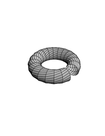
Figure 3: A Dehn twist of a torus is obtained by cutting along one of the circumferences, rotating one end by $2\pi$, and regluing.

It is easy to see that the mapping class group of a spacetime $M$ acts on $\pi_{1}(M)$, and therefore on the holonomies of subsection 2.1. As a group of diffeomorphisms, the group also acts on the constant curvature metrics $\bar{g}_{ij}$, and hence on the moduli $m_{\alpha}$ of subsection 2.3. Classically, geometries that differ by actions of ${\cal D}(M)$ are completely equivalent, so the “true” space of solutions for a spacetime ${\hbox{{\rm I}\kern-1.99997pt\hbox{\rm R}}}\!\times\!\Sigma$ is really

$$T^{*}{\cal N}(\Sigma)/{\cal D}(\Sigma).$$ (2.38)

Quantum mechanically, this equivalence may be relaxed, but wave functions should at least transform under some unitary representation of the mapping class group.

2.5 The Torus Universe

The discussion so far has been rather abstract. For a concrete example, let us consider the torus universe, $M\!\approx\!{\hbox{{\rm I}\kern-1.99997pt\hbox{\rm R}}}\!\times\!T^{2}$, with a negative cosmological constant $\Lambda\!=\!-1/\ell^{2}$ (see [80, 81] for further details). Our goal is to obtain three distinct descriptions of this set of solutions—in terms of geometric structures, Chern-Simons holonomies, and ADM moduli and momenta—and to understand their relationships. As we shall see in section 3, these three desriptions, although classically equivalent, naturally lead to rather different approaches to quantization.

The fundamental group of ${\hbox{{\rm I}\kern-1.99997pt\hbox{\rm R}}}\!\times\!T^{2}$ has two generators, $[\gamma_{1}]$ and $[\gamma_{2}]$, corresponding to the two independent circumferences of the torus. These satisfy the single relation

$$[\gamma_{1}]\cdot[\gamma_{2}]=[\gamma_{2}]\cdot[\gamma_{1}].$$ (2.39)

The holonomy group $\cal M$ is therefore generated by two commuting $\hbox{SO}(2,2)$ matrices, unique up to overall conjugation. It is somewhat more convenient to describe the holonomies as elements of the covering group $\hbox{SL}(2,{\hbox{{\rm I}\kern-1.99997pt\hbox{\rm R}}})\!\times\!\hbox{SL}(2,{\hbox{{\rm I}\kern-1.99997pt\hbox{\rm R}}})$ [68]; I shall do so below. Since the moduli space of the torus is two-dimensional—it is parametrized by a single complex number $\tau$—we expect from subsection 2.3 that the phase space should be four-dimensional; that is, we should find a four-parameter family of holonomies $\rho$.

Let $\rho^{\pm}[\gamma_{a}]$ denote the two $\hbox{SL}(2,{\hbox{{\rm I}\kern-1.99997pt\hbox{\rm R}}})$ holonomies corresponding to the curve $\gamma_{a}$. An $\hbox{SL}(2,{\hbox{{\rm I}\kern-1.99997pt\hbox{\rm R}}})$ matrix $S$ is called hyperbolic, elliptic, or parabolic according to whether $|\hbox{Tr}S|$ is greater than, equal to, or less than 2, and the space of holonomies correspondingly splits into nine sectors. It may be shown that only the hyperbolic-hyperbolic sector corresponds to a spacetime in which the $T^{2}$ slices are spacelike [59, 82, 83]. By suitable overall conjugation, the two generators of the holonomy group can then be taken to be

$$\rho^{\pm}[\gamma_{1}]=\left(\begin{array}[]{cc}e^{r_{1}^{\pm}/2}&0\\ 0&e^{-r_{1}^{\pm}/2}\end{array}\right)$$ (2.42)

$$\rho^{\pm}[\gamma_{2}]=\left(\begin{array}[]{cc}e^{r_{2}^{\pm}/2}&0\\ 0&e^{-r_{2}^{\pm}/2}\end{array}\right),$$ (2.45)

where the $r_{a}^{\pm}$ are four arbitrary parameters.

To obtain the corresponding geometry, we can use the quotient space construction of subsection 2.1. Note first that three-dimensional anti-de Sitter space is naturally isometric to the group manifold of $\hbox{SL}(2,{\hbox{{\rm I}\kern-1.99997pt\hbox{\rm R}}})$. Indeed, anti-de Sitter space can be represented as the submanifold of flat ${\hbox{{\rm I}\kern-1.99997pt\hbox{\rm R}}}^{2,2}$ (with coordinates $(X_{1},X_{2},T_{1},T_{2})$ and metric $dS^{2}=dX_{1}^{2}+dX_{2}^{2}-dT_{1}^{2}-dT_{2}^{2}$) on which

$$\hbox{det}|{\bf X}|=1,\qquad{\bf X}={1\over\ell}\left(\begin{array}[]{cc}X_{1}+T_{1}&X_{2}+T_{2}\\ -X_{2}+T_{2}&X_{1}-T_{1}\end{array}\right),$$ (2.46)

i.e., ${\bf X}\in\hbox{SL}(2,{\hbox{{\rm I}\kern-1.99997pt\hbox{\rm R}}})$. The quotient of anti-de Sitter space by our holonomy group may be obtained by allowing the $\rho^{+}[\gamma_{a}]$ to act on $\bf X$ by left multiplication and the $\rho^{-}[\gamma_{a}]$ to act by right multiplication. It is not hard to show that the induced metric on the resulting quotient space is

$$ds^{2}=dt^{2} - {\ell^{2}\over 4}\left[(r_{1}^{+})^{2}+(r_{1}^{-})^{2}+2r_{1}^{+}r_{1}^{-}\cos{2t\over\ell}\right]dx^{2}$$

$$\qquad-{\ell^{2}\over 2}\left[r_{1}^{+}r_{2}^{+}+r_{1}^{-}r_{2}^{-}+(r_{1}^{+}r_{2}^{-}+r_{1}^{-}r_{2}^{+})\cos{2t\over\ell}\right]dxdy$$

$$\qquad\qquad-{\ell^{2}\over 4}\left[(r_{2}^{+})^{2}+(r_{2}^{-})^{2}+2r_{2}^{+}r_{2}^{-}\cos{2t\over\ell}\right]dy^{2},$$

where $x$ and $y$ are coordinates with period $1$.

It is easy to confirm that the metric (2.5) is indeed that of a space of constant negative curvature. To relate this result to the Chern-Simons picture, observe that the corresponding triad and spin connection are

$$e^{0} = dt$$

$$e^{1} = {\ell\over 2}\left[(r_{1}^{+}-r_{1}^{-})dx+(r_{2}^{+}-r_{2}^{-})dy\right]\sin{t\over{\ell}}$$ (2.48)

$$e^{2} = {\ell\over 2}\left[(r_{1}^{+}+r_{1}^{-})dx+(r_{2}^{+}+r_{2}^{-})dy\right]\cos{t\over{\ell}}$$

$$\omega^{12} = 0$$

$$\omega^{01} = -{1\over 2}\left[(r_{1}^{+}-r_{1}^{-})dx+(r_{2}^{+}-r_{2}^{-})dy\right]\cos{t\over{\ell}}$$ (2.49)

$$\omega^{02} = {1\over 2}\left[(r_{1}^{+}+r_{1}^{-})dx+(r_{2}^{+}+r_{2}^{-})dy\right]\sin{t\over{\ell}}.$$

These can be used to construct a pair of $\hbox{SL}(2,{\hbox{{\rm I}\kern-1.99997pt\hbox{\rm R}}})$ gauge fields $A^{(\pm)a}$ as in (2.22), and it is not hard to check that these have vanishing field strength. Conversely, the holonomies of the $A^{(\pm)a}$ may be shown to reproduce (2.45), as required for consistency.

These expressions may in turn be related to the ADM formalism of subsection 2.3. For the metric (2.5), the extrinsic curvature of a slice of constant $t$ is

$$T=-{d\over dt}\ln\sqrt{g}=-{2\over\ell}\cot{2t\over\ell},$$ (2.50)

which is monotonic in $t$ in the range $(0,\pi\ell/2)$ and is independent of $x$ and $y$. Constant $t$ slices are thus also slices of constant York time. The modulus of a slice of constant $t$ is easily computed by comparing (2.5) to (2.31); one obtains

$$\tau=\left(r_{1}^{-}e^{it/\ell}+r_{1}^{+}e^{-{it/\ell}}\right)\left(r_{2}^{-}e^{it/\ell}+r_{2}^{+}e^{-{it/\ell}}\right)^{\lower 2.0pt\hbox{$\scriptstyle-1$}}.$$ (2.51)

The conjugate momentum $p=p^{1}+ip^{2}$ can be similarly computed from the extrinsic curvature of a constant $t$ slice, using (2.36); it takes the form

$$p=-{i\ell\over 2\sin{2t\over\ell}}\left(r_{2}^{+}e^{it/\ell}+r_{2}^{-}e^{-{it/\ell}}\right)^{\lower 2.0pt\hbox{$\scriptstyle 2$}}.$$ (2.52)

Finally, the ADM Hamiltonian $H$ may also be obtained from the metric, using (2.35):

$$H=\left(T^{2}+{4\over\ell^{2}}\right)^{-1}[\tau_{2}{}^{2}p\bar{p}]^{1/2}={\ell^{2}\over 4}\sin{2t\over\ell}(r_{1}^{-}r_{2}^{+}-r_{1}^{+}r_{2}^{-}).$$ (2.53)

In the limit of vanishing cosmological constant, these relations go over to those of [84] (see [80]).

Let us next consider the Poisson brackets among these variables. From the brackets (2.25), we find that

$$\{r_{1}^{\pm},r_{2}^{\pm}\}=\mp{1\over\ell},\qquad\{r^{+}_{a},r^{-}_{b}\}=0.$$ (2.54)

The corresponding brackets among the moduli and momenta $\tau$ and $p$ may be computed from (2.51) and (2.52); we obtain

$$\{\tau,\bar{p}\}=\{\bar{\tau},p\}=2,\quad\{\tau,p\}=\{\bar{\tau},\bar{p}\}=0,$$ (2.55)

in agreement with (2.37). It may also be shown that these brackets lead to a set of Hamilton’s equations of motion that reproduce the time dependence (2.51) of the moduli. (See [80, 85] for a more detailed description of the dynamics.) Our various descriptions thus all agree, as they must.

It is also useful to exhibit the Poisson brackets among the traces of the holonomies, which serve as a set of gauge-invariant observables. Let

$$R_{1}^{\pm} = {1\over 2}\hbox{Tr}\rho^{\pm}[\gamma_{1}]=\cosh{r_{1}^{\pm}\over 2},$$

$$R_{2}^{\pm} = {1\over 2}\hbox{Tr}\rho^{\pm}[\gamma_{2}]=\cosh{r_{2}^{\pm}\over 2},$$ (2.56)

$$R_{12}^{\pm} = {1\over 2}\hbox{Tr}\rho^{\pm}[\gamma_{1}\cdot\gamma_{2}]=\cosh{(r_{1}^{\pm}+r_{2}^{\pm})\over 2}.$$

It is then not hard to check that

$$\{R_{1}^{\pm},R_{2}^{\pm}\}=\mp{1\over{4\ell}}(R_{12}^{\pm}-R_{1}^{\pm}R_{2}^{\pm})\quad\hbox{\it and cyclical permutations},$$ (2.57)

reproducing the Poisson algebra of Nelson, Regge, and Zertuche [68].

Finally, let us consider the action of the torus mapping class group. This group is generated by two Dehn twists, which act on $\pi_{1}(T^{2})$ by

$$S :\gamma_{1}\rightarrow\gamma_{2}^{-1},\hphantom{\gamma_{2}}\qquad\gamma_{2}\rightarrow\gamma_{1}$$ (2.58)

$$T :\gamma_{1}\rightarrow\gamma_{1}\cdot\gamma_{2},\qquad\gamma_{2}\rightarrow\gamma_{2}.$$

These transformations act on the parameters $r_{a}^{\pm}$ as

$$S :r_{1}^{\pm}\rightarrow r_{2}^{\pm},\hphantom{+r_{2}^{\pm}r}\!\qquad r_{2}^{\pm}\rightarrow-r_{1}^{\pm}$$ (2.59)

$$T :r_{1}^{\pm}\rightarrow r_{1}^{\pm}+r_{2}^{\pm},\qquad r_{2}^{\pm}\rightarrow r_{2}^{\pm},$$

and on the ADM moduli and momenta as

$$S :\tau\rightarrow-{1\over\tau},\hphantom{1}\qquad p\rightarrow\bar{\tau}^{2}p$$ (2.60)

$$T :\tau\rightarrow\tau+1,\qquad p\rightarrow p.$$

It is not hard to show that these transformations are consistent with the relationships between the ADM and holonomy variables, and that they preserve all Poisson brackets.

2.6 The (2+1)-Dimensional Black Hole

I will finish this section by describing another exact solution with a negative cosmological constant, the (2+1)-dimensional black hole. The discovery of this solution by Bañados, Teitelboim, and Zanelli (BTZ) [86, 87] came as a surprise, since it had been generally assumed that physically realistic solutions required the full dynamics of 3+1 dimensions. Indeed, the (2+1)-dimensional black hole differs from its (3+1)-dimensional counterpart in one important way: since the spacetime curvature is constant in 2+1 dimensions, there can be no curvature singularity at the origin. Nevertheless, the BTZ solution shares many of the essential features of a realistic black hole, including an event horizon, an inner horizon (in the rotating case), and thermodynamic properties.

Like the torus universe, the black hole has a geometry that can be described in several different languages. The relationship to the ordinary Schwarzschild and Kerr black holes is most easily exhibited in the metric formalism. The BTZ metric is

$$ds^{2}=-(N^{\perp})^{2}dt^{2}+f^{-2}dr^{2}+r^{2}\left(d\phi+N^{\phi}dt\right)^{2}$$ (2.61)

with lapse and shift functions

$$N^{\perp}=f=\left(-M+{r^{2}\over\ell^{2}}+{J^{2}\over 4r^{2}}\right)^{1/2},\qquad N^{\phi}=-{J\over 2r^{2}}\ .$$ (2.62)

Here, the time coordinate $t$ is not the York time of subsection 2.3, but is rather the “Killing time,” the displacement along a timelike Killing vector at spatial infinity. (The analysis in terms of York time is possible, but considerably more complicated [88].) It is straightforward to check that the metric (2.61) satisfies the Einstein field equations with a cosmological constant $\Lambda=-1/\ell^{2}$.

When $M\!>\!0$ and $|J|\!\leq\!M\ell$, this solution has an outer event horizon at $r=r_{+}$ and an inner horizon at $r=r_{-}$, where

$$r_{\pm}^{2}={M\ell^{2}\over 2}\left\{1\pm\left[1-\left({J\over M\ell}\right)^{2}\right]^{1/2}\right\},$$ (2.63)

i.e.,

$$M={r_{+}^{2}+r_{-}^{2}\over\ell^{2}},\quad J={2r_{+}r_{-}\over\ell}\ .$$ (2.64)

The parameters $M$ and $J$ can be studied either by looking at spatial integrals at infinity [87] or by examining quasilocal expressions at a finite spatial boundary [89]; either analysis shows that they are simply the mass and angular momentum of the black hole.

Since the black hole metric has constant negative curvature, it must be at least locally isometric to anti-de Sitter space. For the region $r\!>\!r_{+}$, this isometry may be exhibited by means of a coordinate change (the corresponding transformations for $r\!<\!r_{+}$ are given in [87]; see also [90]):

$$x = \left({r^{2}-r_{+}^{2}\over r^{2}-r_{-}^{2}}\right)^{1/2}\cosh\left({r_{+}\over\ell^{2}}t-{r_{-}\over\ell}\phi\right)\exp\left\{{r_{+}\over\ell}\phi-{r_{-}\over\ell^{2}}t\right\}$$

$$y = \left({r^{2}-r_{+}^{2}\over r^{2}-r_{-}^{2}}\right)^{1/2}\sinh\left({r_{+}\over\ell^{2}}t-{r_{-}\over\ell}\phi\right)\exp\left\{{r_{+}\over\ell}\phi-{r_{-}\over\ell^{2}}t\right\}$$ (2.65)

$$z = \left({r_{+}^{2}-r_{-}^{2}\over r^{2}-r_{-}^{2}}\right)^{1/2}\exp\left\{{r_{+}\over\ell}\phi-{r_{-}\over\ell^{2}}t\right\},$$

for which the metric becomes

$$ds^{2}={\ell^{2}\over z^{2}}(dx^{2}-dy^{2}+dz^{2}).$$ (2.66)

This expression may be recognized as the standard Poincaré metric for anti-de Sitter space. Note, however, that periodicity in the Schwarzschild angular coordinate $\phi$ requires that we identify points under the action $\phi\!\mapsto\!\phi+2\pi$, that is,

$$( x,y,z)\sim$$

$$\left(e^{2\pi r_{+}/\ell}(x\cosh{2\pi r_{-}\over\ell}-y\sinh{2\pi r_{-}\over\ell}),\,e^{2\pi r_{+}/\ell}(y\cosh{2\pi r_{-}\over\ell}-x\sinh{2\pi r_{-}\over\ell}),\,e^{2\pi r_{+}/\ell}z\right)$$

These identifications are an isometry of the metric (2.66), and thus represent an element of the isometry group $\hbox{SL}(2,{\hbox{{\rm I}\kern-1.99997pt\hbox{\rm R}}})\!\times\!\hbox{SL}(2,{\hbox{{\rm I}\kern-1.99997pt\hbox{\rm R}}})$ of anti-de Sitter space. This element is, in fact, the holonomy of the geometric structure of the black hole in the sense of subsection 2.1. The corresponding $\hbox{SL}(2,{\hbox{{\rm I}\kern-1.99997pt\hbox{\rm R}}})$ matrices $\rho^{\pm}$ may be obtained from the group action described after equation (2.46); a bit of computation gives

$$\rho^{\pm}=\left(\begin{array}[]{cc}e^{\pi r_{\pm}/\ell}&0\\ 0&e^{-\pi r_{\pm}/\ell}\end{array}\right).$$ (2.68)

The $\hbox{SL}(2,{\hbox{{\rm I}\kern-1.99997pt\hbox{\rm R}}})$ Chern-Simons connections (2.22) can also be obtained from (2.66)–(2.6), and it is a simple exercise to check that the holonomy of the connection is the same as the holonomy of the geometric structure. This holonomy was originally computed in the Schwarzschild coordinates (2.61) in reference [91]; the resulting expression differs from (2.68) by a complicated overall conjugation. Note that the Poisson brackets for the black hole spacetime are rather mysterious: the parameters $r_{+}$ and $r_{-}$ are independent, and seem to have no canonical conjugates. We shall return to this issue in subsection 4.1.

3. Quantum Gravity in 2+1 Dimensions

The main goal of studying general relativity in (2+1) dimensions is to gain insight into the problems of quantum gravity. It may therefore seem that I have spent an inordinate amount of time on the details of the classical theory. We shall see, however, that the three classical descriptions of the last section lead very directly to three approaches to quantization. Indeed, one of the main lessons of (2+1)-dimensional gravity seems to be that a thorough understanding of the classical solutions is crucial for the formulation of a quantum theory.

Before starting in on the problem of quantization, it is worth recalling why quantum gravity is so hard. The difficulties are partly technical: general relativity is a complicated, nonlinear theory, and approximation methods that work elsewhere simply break down. In particular, general relativity is perturbatively nonrenormalizable, and while we know a few examples of nonrenormalizable theories that can be sensibly quantized, the general problem is poorly understood.

Beyond these technical failures, however, lie the basic conceptual problems that plague quantum gravity. Conventional quantum theory starts with a fixed, passive spacetime background that provides a setting in which particles and fields interact. According to general relativity, however, spacetime is itself dynamical, and much of the conventional framework becomes, at best, ambiguous. Without a fixed definition of time, we do not know how to describe dynamics or interpret probabilities. Without an a priori distinction between past, present, and future, we do not how to impose causality. Fundamentally, we do not understand what it means to quantize the structure of spacetime.

The usefulness of (2+1)-dimensional gravity comes from the fact that it eliminates the technical problems while preserving the conceptual foundations. We have seen that for typical topologies, (2+1)-dimensional general relativity has only finitely many degrees of freedom. Quantum field theory is thus reduced to quantum mechanics, and the problem of nonrenormalizability disappears. On the other hand, (2+1)-dimensional gravity is still a diffeomorphism-invariant theory of spacetime geometry, and most of the basic conceptual issues of the full theory remain unchanged.

To describe the quantization of (2+1)-dimensional general relativity, I will work backwards through the classical descriptions of the previous section, starting with the ADM formalism and ending with the quantum mechanics of geometric structures. A final subsection will briefly address some other approaches to quantization, including path integral methods and lattice approaches.

3.1 Reduced Phase Space Quantization

Perhaps the simplest approach to quantum gravity in 2+1 dimensions [84, 92] starts from the reduced phase space action (2.34), which was obtained by solving the constraints in the metric formalism. This action describes a finite-dimensional system in classical mechanics, albeit one with a complicated, time-dependent Hamiltonian. We know, at least in principle, how to quantize such a system: we simply replace the Poisson brackets (2.37) with commutators,

$$[\hat{m}_{\alpha},\hat{p}^{\beta}]=i\hbar\delta^{\beta}_{\alpha},$$ (3.1)

represent the momenta as derivatives,

$$p^{\alpha}={\hbar\over i}{\partial\ \over\partial m_{\alpha}},$$ (3.2)

and choose our wave functions to be square integrable functions $\psi(m_{\alpha},T)$ that evolve according to the Schrödinger equation

$$i\hbar{\partial\psi(m_{\alpha},T)\over\partial T}=\hat{H}\psi(m_{\alpha},T),$$ (3.3)

where the Hamiltonian $\hat{H}$ is obtained from (2.35) by some suitable operator ordering. Invariance under the mapping class group can be incorporated by demanding that the $\psi(m_{\alpha},T)$ transform under a suitable representation of ${\cal D}(M)$; a similar requirement can help determine the operator ordering in the Hamiltonian operator, although some ambiguities will remain.

For spatial surfaces of genus $g\!>\!2$, the complexity of the constraint (2.33)—which must be solved to determine $\hat{H}$—may make this approach to quantization impractical. A perturbative expression for $\hat{H}$ might still exist, however, and Puzio has suggested that the Gauss map could provide a useful tool [93]. For spaces of genus 2, there is some hope that the representation of $\Sigma$ as a hyperelliptic surface could lead to an exact solution of the constraint; and for the genus 1 case, the exact expression for $\hat{H}$ is already known.

Indeed, the classical Hamiltonian for the torus universe is given by equation (2.53), which yields, up to operator ordering ambiguities,

$$\hat{H}={\hbar\over\sqrt{T^{2}-4\Lambda}}\Delta_{0}^{1/2},$$ (3.4)

where

$$\Delta_{0}=-\tau_{2}^{\ 2}\left({\partial^{2}\ \over\partial\tau_{1}^{\ 2}}+{\partial^{2}\ \over\partial\tau_{2}^{\ 2}}\right)$$ (3.5)

is the ordinary scalar Laplacian for the constant negative curvature Poincaré metric on moduli space. This Laplacian is invariant under the modular transformations (2.60), and its invariant eigenfunctions, known as weight zero Maass forms, have been studied rather carefully in the mathematical literature [94]. The behavior of the corresponding wave functions is discussed by Puzio [95], who argues that they are well-behaved at the “edges” of moduli space.

While the choice (3.5) of operator ordering is not unique, the number of possible alternatives is smaller than one might naively expect. The key restriction is diffeomorphism invariance: the eigenfunctions of the Hamiltonian should transform under a one-dimensional unitary representation of the mapping class group. The representation theory of the modular group (2.60) has been studied extensively [96, 97]; one finds that the possible inequivalent Hamiltonians are all of the form (3.4), but with $\Delta_{0}$ replaced by

$$\Delta_{n}=-\tau_{2}^{\ 2}\left({\partial^{2}\ \over\partial\tau_{1}^{\ 2}}+{\partial^{2}\ \over\partial\tau_{2}^{\ 2}}\right)+2in\tau_{2}{\partial\ \over\partial\tau_{1}}+n(n+1),\quad 2n\in{\hbox{{\rm Z}\kern-3.99994pt\hbox{\rm Z}}},$$ (3.6)

the Maass Laplacian acting on automorphic forms of weight $n$. (See [99] for details of the required operator orderings.) Note that when written in terms of the momentum $p$, the operators $\Delta_{n}$ differ from each other by terms of order $\hbar$, as expected for operator ordering ambiguities. Nevertheless, the various choices of ordering may have drastic effects on the physics, since the spectra of the various Maass Laplacians are quite different.

This ordering ambiguity may be viewed as arising from the structure of the classical phase space. The torus moduli space is not a manifold, but rather has orbifold singularities, and quantization on an orbifold is generally not unique. Since the space of solutions of the Einstein equations in 3+1 dimensions has a similar orbifold structure [100], we might expect a similar ambiguity in realistic (3+1)-dimensional quantum gravity.

The quantization presented here is an example of what Kuchař calls an “internal Schrödinger interpretation” [101]. It appears to be a completely self-consistent approach, and like ordinary quantum mechanics, it automatically has the correct classical limit on the reduced phase space of subsection 2.3. The key drawback of this approach is that it relies on a classical choice of time slicing. The analysis of subsection 2.3 required that we choose the York time slicing from the start, and it is not at all clear that a different choice would lead to an equivalent quantum theory. In other words, it is not clear that this approach to quantum gravity preserves general covariance.

The problem may be rephrased as a statement about the kinds of questions we can ask in this quantum theory. The model naturally allows us to compute the transition amplitude between the spatial geometry of a time slice of constant mean curvature $-\hbox{Tr}K\!=\!T_{1}$ and the geometry of a later slice of constant mean curvature $-\hbox{Tr}K\!=\!T_{2}$. But it is not clear how to ask for transition amplitudes among other spatial slices, on which $\hbox{Tr}K$ is not constant; such questions would require a different classical time slicing, and hence a different—and perhaps inequivalent—quantum theory.

To try to escape this difficulty, we next turn to an alternative approach to quantization, which starts from the Chern-Simons formalism.

3.2 Chern-Simons Quantum Theory

In the first-order formulation of subsection 2.2, the fundamental gauge-invariant observables of quantum gravity are the traces $\hbox{Tr}\rho[\gamma]$ of the holonomies. These provide an overcomplete set of coordinates for the space of classical solutions, and it is not obvious that the entire set of Poisson brackets can be made into commutators of operators. This problem has been studied systematically by Nelson and Regge [63, 64, 65, 68, 102, 103, 104], who demonstrate the existence of a well-behaved subalgebra of traces for which commutators can be consistently defined.

For the case of the torus universe, this approach is fairly straightforward. To quantize the algebra (2.57), we proceed as follows:

1. We replace the classical Poisson brackets $\{\,,\,\}$ by commutators $[\,,\,]$, with the rule

   $$[x,y]=xy-yx=i\hbar\{x,y\};$$

2. On the right hand side of (2.57), we replace the product by the symmetrized product,

   $$xy\to{1\over 2}(xy+yx).$$

The resulting algebra is defined by the relations

$$\hat{R}_{1}^{\pm}\hat{R}_{2}^{\pm}e^{\pm i\theta}-\hat{R}_{2}^{\pm}\hat{R}_{1}^{\pm}e^{\mp i\theta}=\pm 2i\sin\theta\,\hat{R}_{12}^{\pm}\quad\hbox{\it and cyclical permutations}$$ (3.7)

with

$$\tan\theta=-{\hbar\over 8\ell}\ .$$ (3.8)

The algebra (3.7) is not a Lie algebra, but it is related to the Lie algebra of the quantum group $\hbox{SU}_{q}(2)$ [68], with $q=\exp{4i\theta}$.

In terms of the parameters $r_{a}^{\pm}$ of subsection 2.5, this algebra can be represented by [80, 81]

$$\hat{R}_{1}^{\pm}=\sec\theta\cosh{\hat{r}_{1}^{\pm}\over 2},\quad\hat{R}_{2}^{\pm}=\sec\theta\cosh{\hat{r}_{2}^{\pm}\over 2},\quad\hat{R}_{12}^{\pm}=\sec\theta\cosh{(\hat{r}_{1}^{\pm}+\hat{r}_{2}^{\pm})\over 2}$$ (3.9)

with

$$[\hat{r}_{1}^{\pm},\hat{r}_{2}^{\pm}]=\pm 8i\theta,\qquad[\hat{r}^{+}_{a},\hat{r}^{-}_{b}]=0.$$ (3.10)

For $\Lambda$ small, these commutators differ from the naive quantization of the classical brackets (2.54),

$$[\hat{r}_{1}^{\pm},\hat{r}_{2}^{\pm}]=\mp{i\hbar\over\ell},$$ (3.11)

by terms of order $\hbar^{3}$.

We must next implement the action of the modular group (2.59) on the operators $\hat{R}^{\pm}_{a}$. The action that preserves the algebraic relations (3.7) is

$$S :\hat{R}_{1}^{\pm}\rightarrow\hat{R}_{2}^{\pm},\quad\hat{R}_{2}^{\pm}\rightarrow\hat{R}_{1}^{\pm},\quad\hat{R}_{12}^{\pm}\rightarrow\hat{R}_{1}^{\pm}\hat{R}_{2}^{\pm}+\hat{R}_{2}^{\pm}\hat{R}_{1}^{\pm}-\hat{R}_{12}^{\pm}$$ (3.12)

$$T :\hat{R}_{1}^{\pm}\rightarrow\hat{R}_{12}^{\pm},\quad\hat{R}_{2}^{\pm}\rightarrow\hat{R}_{2}^{\pm},\quad\hat{R}_{12}^{\pm}\rightarrow\hat{R}_{12}^{\pm}\hat{R}_{2}^{\pm}+\hat{R}_{2}^{\pm}\hat{R}_{12}^{\pm}-\hat{R}_{1}^{\pm},$$

which may be recognized as a particular factor ordering of the classical group action.

This approach to quantization is an example of what Kuchař calls “quantum gravity without time” [101]. Like the quantization of subsection 3.1, it appears to be self-consistent, but like that approach, it suffers from an important deficiency. In this case, the observables $\hat{R}_{a}$ characterize the entire spacetime at once, and are therefore time-independent constants of motion. But the classical solutions to (2+1)-dimensional gravity, even for the simple ${\hbox{{\rm I}\kern-1.99997pt\hbox{\rm R}}}\!\times\!T^{2}$ topology, are most certainly not static. Our operators have somehow lost track of the dynamics of spacetime.

As in subsection 3.1, the problem can be phrased as a limitation on the kinds of questions we can ask. In this quantization, we can ask about the overall spacetime geometry, but we have apparently lost the ability to describe dynamics. This “frozen time” problem is characteristic of generally covariant theories: translations in (coordinate) time are diffeomorphisms, and cannot be seen by looking at diffeomorphism-invariant observables. Rovelli has suggested a solution to this difficulty, based on the idea of “evolving constants of motion” [105, 106]. To see this method in action, it is useful to turn to yet another approach to quantum gravity, that of covariant canonical quantization.

3.3 Covariant Canonical Quantization

The starting point of covariant canonical quantization [107, 108, 109, 110] is the simple but profound observation that the phase space of any well-behaved classical theory is isomorphic to the space of classical solutions. Specifically, let $\cal C$ be an arbitrary (but fixed) Cauchy surface. Then a point in the phase space determines initial data on $\cal C$, which in turn determine a unique solution, while, conversely, a classical solution restricted to $\cal C$ determines a point in the phase space. This observation suggests a solution of the old “covariant vs. canonical” debate in quantum gravity [111], by offering a manifestly covariant approach to canonical quantization.

For (2+1)-dimensional gravity on a spacetime with the topology ${\hbox{{\rm I}\kern-1.99997pt\hbox{\rm R}}}\!\times\!\Sigma$, we saw in subsection 2.1 that the space of classical solutions of the vacuum field equations is the simply the space $T^{*}{\cal N}(\Sigma)/{\cal D}(\Sigma)$ of holonomies of geometric structures. As a cotangent bundle, this space has a natural symplectic structure, and it follows from the results of subsection 2.2 (see equations (2.16)–(2.17) and (2.25)) that this structure is closely related to the symplectic structure of the classical Poisson brackets. When $\Lambda\!\neq\!0$, the cotangent bundle structure disappears, but the structure of the fundamental group of a surface induces a symplectic structure on ${\cal M}/{\cal D}$, which is again closely related to the classical Poisson bracket structure. As Goldman has shown [70, 71], this symplectic structure may be described abstractly in terms of Poisson brackets among intersecting loops on $\Sigma$, with added relations that depend on the “gauge group” $G$ of the geometric structure. For any particular parametrization of $\cal M$, explicit expressions for the brackets among parameters may be determined from Chern-Simons quantization or from the operator algebras of Nelson and Regge. For the ${\hbox{{\rm I}\kern-1.99997pt\hbox{\rm R}}}\!\times\!T^{2}$ universe, for example, the $r_{a}^{\pm}$ can be interpreted as coordinates on $\cal M$, and the brackets (2.54) determine a symplectic structure on this space.

To quantize this covariant phase space, we must rewrite a suitable subalgebra of classical Poisson brackets as commutators. We are thus led to a quantum theory in which wave functions are functions of the holonomies $\hat{\rho}\!\in\!{\cal N}$, or, if $\Lambda\!\neq\!0$, of a suitably chosen set of half of the coordinates of $\cal M$. For the torus universe, for instance, we obtain operators $\hat{r}_{a}^{\pm}$ satisfying the commutation relations (3.11), and wave functions of the form $\psi(r_{1}^{+},r_{1}^{-})$. (To recover the results of reference [84] in the limit $\Lambda\!\rightarrow\!0$, we should choose a different “polarization,” writing wave functions as functions of the commuting variables $u_{1}$ and $u_{2}$, where $u_{a}=(r^{+}_{a}-r^{-}_{a})/2$; see [80] for details.)

Like the Chern-Simons quantization of the last subsection, covariant canonical quantization leads to a “frozen time” formalism, in which the fundamental operators are constants of motion that describe an entire classical spacetime. It should be clear, however, that this is not just a problem of the quantization: our classical description of the phase space is already time-independent. But we know how to solve this problem in the classical theory: we simply make use of the isomorphism between the covariant canonical description and the conventional time-dependent description of the phase space.

Let me rephrase this idea, as it applies to (2+1)-dimensional gravity, in a slightly less abstract manner. Given a (time-independent) holonomy $\rho$ of a geometric structure, we can reconstruct a unique classical spacetime. Within that spacetime, we can ask ordinary dynamical questions: for instance, what are the moduli of the slice of York time $-\hbox{Tr}K=T$? Indeed, for the torus universe, this is precisely the content of equation (2.51), which gives the modulus of a torus of fixed $T$ in terms of the coordinates $r_{a}^{\pm}$ of the geometric structure. Similarly, given any other time slicing, the question “What are the moduli of the time $T^{\prime}$ slice?” has a unique classical answer, depending only on $\rho$ and $T^{\prime}$.

To carry this construction over to the quantum theory, we need merely convert equation (2.51), and its counterparts for other time-dependent observables, into operator relations. For example, we can define a one-parameter family of operators $\hat{\tau}(t)$ by

$$\hat{\tau}(t)=\left(\hat{r}_{1}^{-}e^{it/\ell}+\hat{r}_{1}^{+}e^{-{it/\ell}}\right)\left(\hat{r}_{2}^{-}e^{it/\ell}+\hat{r}_{2}^{+}e^{-{it/\ell}}\right)^{\lower 2.0pt\hbox{$\scriptstyle-1$}},$$ (3.13)

where $t$ is now simply a label whose physical significance comes from the classical limit. Similarly, we can use equation (2.52) to define a second one-parameter family of operators that represent the ADM momenta on a slice of constant York time,

$$\hat{p}(t)=-{i\ell\over 2\sin{2t\over\ell}}\left(\hat{r}_{2}^{+}e^{it/\ell}+\hat{r}_{2}^{-}e^{-{it/\ell}}\right)^{\lower 2.0pt\hbox{$\scriptstyle 2$}};$$ (3.14)

and from (2.53), we can define a third family representing the Hamiltonian that generates translations in York time,

$$\hat{H}(t)={\ell^{2}\over 4}\sin{2t\over\ell}(\hat{r}_{1}^{-}\hat{r}_{2}^{+}-\hat{r}_{1}^{+}\hat{r}_{2}^{-}).$$ (3.15)

It may be checked that these operators obey the standard Heisenberg equations of motion, and that they transform correctly under the mapping class group. (The requirement of simple behavior under the action of the mapping class group was, in fact, a key ingredient in determining the operator orderings.)

If we are given a different classical time slicing, labeled by a new coordinate $T^{\prime}$, we can repeat this procedure, using the classical solutions to construct new operators $\{\hat{\tau}^{\prime}(T^{\prime}),\hat{p}^{\prime}(T^{\prime}),\hat{H}^{\prime}(T^{\prime})\}$, which again act on the Hilbert space of the covariant canonical quantum theory. From this viewpoint, the “frozen time” problem is simply a sign that covariant canonical quantization leads to a Heisenberg picture, in which wave functions are time-independent; the dynamics now lies in our choice of families of operators. Of course, this construction involves operator ordering ambiguities, and exact expressions for the “time-dependent” operators require our knowing the exact solutions of the classical field equations. But these problems are in some sense technical, and perhaps not fundamental.

Finally, let me relate the results of this subsection to those of subsections 3.1 and 3.2. The connection to Chern-Simons quantization is straightforward: equation (3.9) expresses the Chern-Simons operators in terms of the $\hat{r}_{a}^{\pm}$, and if we choose the commutators (3.10), we recover the Nelson-Regge operator algebra. To connect covariant canonical quantization to the “internal Schrödinger interpretation” of subsection 3.1, we must transform from a Heisenberg picture to a Schrödinger picture by diagonalizing the operators $\hat{\tau}(t)$. It is easy to construct a formal integral transform to do so (see [98] and [112] for details); one obtains wave functions that formally obey the Schrödinger equation (3.3), but with a Hamiltonian determined by (3.6) with $n=1/2$. Peldan has recently pointed out one potential problem with this transformation, however [113]: the torus mapping class group does not act properly discontinuously on the “configuration spaces” parametrized by $(r_{1}^{+},r_{1}^{-})$ or $(u_{1},u_{2})$, so invariant wave functions cannot be taken to be smooth functions of these configuration space variables. I do not know a resolution to this problem; it may be that the requirement of smoothness is too strong, but further work is needed.

3.4 Other Approaches to Quantization

Let me complete this section by briefly mentioning a few other approaches to quantum gravity in 2+1 dimensions. I cannot hope to do these methods justice in the limited space available; this subsection should be interpreted as a “reading list.” For an earlier review of some of these quantum theories, see reference [114].

1. The Wheeler-DeWitt Equation
   

   One conventional approach to quantum gravity is that of the Wheeler-DeWitt equation. This approach starts with the ADM decomposition of subsection 2.3, but rather than choosing a time slicing and solving the Hamiltonian constraint ${\cal H}\!=\!0$ classically, we impose it as a Klein-Gordon-like equation of motion restricting physical states $\Psi[\bar{g}_{ij},\lambda]$. For the torus universe, this constraint takes the form of a functional differental equation [115]

   $$\Biggl{\{} {\displaystyle{1\over 8}} {\delta\ \over\delta\lambda}e^{-2\lambda}{\delta\ \over\delta\lambda}+{1\over 2}e^{-2\lambda}\Delta_{0}+2\bar{\Delta}\lambda-2e^{-2\lambda}Y^{i}[\pi]\bar{\Delta}Y_{i}[\pi]$$

   $$+ 2e^{-2\lambda}\,\overline{\mathop{\!\nabla\!}}\,_{i}\Biggl{[}\left(2p^{ij}+\,\overline{\mathop{\!\nabla\!}}\,^{i}Y^{j}[\pi]+\,\overline{\mathop{\!\nabla\!}}\,^{j}Y^{i}[\pi]-\bar{g}^{ij}\,\overline{\mathop{\!\nabla\!}}\,_{k}Y^{k}[\pi]\right)Y_{j}[\pi]\Biggr{]}\Biggr{\}}\Psi[\lambda,\tau]=0,$$

   where $Y_{i}[\pi]$ is given by

   $$Y_{i}=-{1\over 2}\bar{\Delta}^{-1}\left[{1\over\sqrt{\bar{g}}}e^{2\lambda}\,\overline{\mathop{\!\nabla\!}}\,_{i}\left(e^{-2\lambda}\pi\right)\right]$$ (3.17)

   and

   $$\pi=-{i\over 2}{\delta\ \over\delta\lambda},\quad p^{ij}=-{i\over\sqrt{\bar{g}}}{\delta\ \over\delta\bar{g}_{ij}}\ .$$ (3.18)

   Note the appearance of nonlocal terms, those involving the $Y_{i}$, which arise from solving the momentum constraints ${\cal H}_{i}=0$. The existence of such nonlocal behavior was first pointed out by Henneaux [116]. The properties of equation (1), and proposals for an inner product for the $\Psi[\lambda,\tau]$, are discussed in [115]; the results do not appear to be equivalent to those of any of the quantizations discussed above, but operator ordering ambiguities in (1) are severe enough that we cannot be certain of this claim. See also [117, 118] for “gauge-fixed” versions of the Wheeler-DeWitt equation, which are essentially minisuperspace models that eliminate the nonlocal terms in (1).

2. Loop Variables
   

   The Chern-Simons variables of subsection 2.2 are, roughly speaking, the (2+1)-dimensional analogues of Ashtekar’s variables in 3+1 dimensions [119, 120]. Work on these variables has led to an interesting “dual” representation, the loop representation [121], in which wave functions and operators are functionals of loops. Wave functions in the loop representation are related to those in the “connection representation” by the loop transform, defined formally as the functional integral

   $$\tilde{\Psi}[\gamma]=\int[d\omega]\,\hat{\rho}[\gamma][\omega]\Psi[\omega],$$ (3.19)

   where $\hat{\rho}[\gamma][\omega]$ is the Wilson loop (2.15). In 2+1 dimensions (with vanishing cosmological constant), $\omega$ is a flat connection, and the wave function $\tilde{\Psi}[\gamma]$ depends only on the homotopy class of $\gamma$. For the torus, in particular, any loop is determined up to homotopy by two winding numbers—in terms of the basis of subsection 2.5,

   $$\gamma\approx\gamma_{1}^{n_{1}}\cdot\gamma_{2}^{n_{2}}.$$ (3.20)

   Wave functions in the loop representation are thus functions $\psi(n_{1},n_{2})$ of a pair of integers, and the loop transform reduces to an ordinary Laplace transform [122, 123]. As Marolf has shown [122], this transform is not an isomorphism, and the loop representation for ${\hbox{{\rm I}\kern-1.99997pt\hbox{\rm R}}}\!\times\!T^{2}$ is consequently inequivalent to the “connection representation” of Chern-Simons quantization. On the other hand, the integration measure in (3.19) can be redefined—although in a rather unpleasant way—to make the transform an isomorphism [124]. There are thus (at least) two loop representations, one equivalent to more conventional quantization and one not.

3. Lattice Methods
   

   We saw in section 2 that the solutions of the vacuum Einstein field equations in 2+1 dimensions are flat. As a consequence, lattice techniques, in which spacetime is approximated by flat polyhedra, are in some sense exact. A number of authors, including Waelbroeck [125, 126, 127], ’t Hooft [14, 128], and Newbury and Unruh [129], have taken advantage of this fact to construct simple lattice models of classical and quantum gravity based on polyhedral decompositions of space or spacetime. These models are for the most part based on the first-order formalism, and should yield quantum theories equivalent to those of subsection 2.2, but the relationships have not been fully explored.

   A second set of lattice models come from Regge calculus. These are based on the old observation of Ponzano and Regge [130, 131] that the (Euclidean) three-dimensional gravitational path integral in Regge calculus variables can be rewritten as a particular sum over 6-j symbols. Turaev and Viro succeeded in regularizing this sum by replacing ordinary 6-j symbols with those of a quantum group [132], and a number of authors [133, 134, 135, 136, 137, 138] have related the states, observables, and expectation values of this model to those of other approaches to quantization. As discussed in reference [114], there are problems with such comparisons, arising from the fact that the Ponzano-Regge action is based on Euclidean gravity; the geometric structures of a manifold with a positive definite metric are quite different from those of a manifold with a Lorentzian metric. Recently, however, Barrett and Foxon have proposed a new approach to the Ponzano-Regge model that may be equivalent to (2+1)-dimensional general relativity with Lorentzian signature [139]; further work on this model could be very interesting.

4. Path Integrals
   

   I will finish this section with a brief discussion of the path integral approach to (2+1)-dimensional gravity, as first developed by Witten [9]. Our starting point is the first-order action (2.10). $I_{\hbox{\scriptsize grav}}$ is not a free field action—it is not quadratic in the fields—but it is nevertheless possible to evaluate the path integral exactly. Roughly speaking, the integral over the triad $e$ gives a delta functional $\delta[R[\omega]]$, where $R^{a}[\omega]$ is the curvature defined by equation (2.14); the delta functional then permits an exact evaluation of the remaining integral over $\omega$. When the Faddeev-Popov determinants that arise from gauge-fixing the ISO(2,1) transformations (2.11)–(2.12) are taken into account, one obtains a partition function consisting of a combination of determinants known as the Ray-Singer torsion,

   $$T[\bar{\omega}]={(\hbox{det}^{\prime}\bar{\Delta}_{(3)})^{3/2}(\hbox{det}^{\prime}\bar{\Delta}_{(1)})^{1/2}\over(\hbox{det}^{\prime}\bar{\Delta}_{(2)})}.$$ (3.21)

   Here $\bar{\omega}$ is a flat connection—the zero of the argument of the delta functional—and $\bar{\Delta}_{(k)}$ is the Laplacian $*D_{\bar{\omega}}\!*\!D_{\bar{\omega}}+D_{\bar{\omega}}\!*\!D_{\bar{\omega}}*$ acting on $k$-forms, where $D_{\bar{\omega}}$ is the covariant derivative. This combination of determinants is a topological invariant of a flat bundle over the spacetime manifold $M$ [140], and is proportional to the Reidemeister torsion, a combinatorial invariant of flat bundles [141, 142]. This same combination of determinants can also be obtained by means of a non-Abelian Hodge decomposition of the “gauge” fields $e$ and $\omega$ [143], or by a BRST analysis of the path integral [144].

   The path integral becomes somewhat more complicated if the Laplacians in (3.21) have zero-modes. This will be the case, for example, if $M$ admits more than one flat connection, as it always does for the topologies we have considered so far. In that case, the partition function will involve an integral of the torsion (3.21) over the moduli space ${\cal M}/{\cal D}$ of flat connections, and will typically acquire infrared divergences. Addition complications arise for spacetimes with boundaries, but the results may still be expressed in terms of standard topological invariants. The full path integral in is considered in all its glory in [145].

   To relate these path integral expressions to the quantizations considered in the subsections 3.1–3.3, we should consider the Ray-Singer torsion for a manifold with the topology $[0,1]\!\times\!\Sigma$, with specified flat connections at the two boundaries $\{0\}\!\times\!\Sigma$ and $\{1\}\!\times\!\Sigma$. It is not hard to show that the result is simply a delta function that equates the initial and final holonomies. The path integral thus reproduces the “frozen time” of Chern-Simons quantization [144].

   We shall see in the next section that more interesting path integrals arise when one considers topology change. Euclidean path integrals have also been used to explore the effects of spacetime topology on the Hartle-Hawking wave function and the partition function in (2+1)-dimensional quantum cosmology [146, 147, 148, 149, 150, 151, 152], and Martinec [153] and Mazur [154] have investigated canonical path integrals in two rather different metric formalisms.

4. Assorted Topics

The previous section gave a brief overview of some of the approaches to quantum gravity in 2+1 dimensions. In this final section, I will briefly discuss two applications of these results: the study of black hole thermodynamics and the investigation of topology-changing amplitudes.

4.1 Black Hole Thermodynamics

Since Hawking’s discovery that quantum mechanical processes cause black holes to radiate [155], black hole thermodynamics has become a natural testing ground for quantum gravity. It is therefore of interest to apply the methods of the last section to the (2+1)-dimensional black hole. Unfortunately, we immediately run into difficulties: as noted at the end of subsection 2.6, the parameters $r_{\pm}$ that determine the geometric structure and the Chern-Simons holonomies for the black hole have no obvious canonical conjugates, and there seems to be no classical Poisson algebra to quantize. This problem arises because the black hole spacetime is not compact; the ordinary Einstein-Hilbert action must be supplemented by boundary terms at infinity and (as a careful analysis shows [90, 156, 157]) at the horizon as well. These boundary terms contain additional parameters that serve as conjugate variables to the $r_{\pm}$.

We can avoid worrying about these boundary terms, however, by making a clever choice of our method of quantization. Rather than using Schwarzschild time $t$ as our time coordinate, let us quantize on surfaces of constant $r$, as is common in conformal field theory [158]. As long as we stay away from the horizons $r=r_{\pm}$ and from spatial infinity, we should not have to deal with boundary terms in such a “radial quantization.”

Let us therefore a consider cylindrical slice of constant $r$ connecting a circle at initial time $t_{1}$ and one at final time $t_{2}$. The geometry of such a slice can no longer be described by the holonomy in the angular direction alone; the Chern-Simons connections $A^{(\pm)}$ now describe parallel transport along open segments between $t_{1}$ and $t_{2}$ as well. The holonomy along a segment $\delta$ starting at $(t_{1},\phi_{1})$ and ending at $(t_{2},\phi_{2})$ will be characterized by two new parameters, $\Delta\phi$ and $\Delta t$. The segment $\delta$ is linked with the closed curve $\gamma$ of subsection 2.6, and the Poisson brackets among $r_{+}$, $r_{-}$, $\Delta\phi$, and $\Delta t$ are consequently nontrivial.

These brackets have been analyzed for the Euclidean black hole in reference [90], where it is shown that they are equivalent to brackets among metric parameters in a minisuperspace model. The Euclidean black hole—which is the configuration relevant for path integral computations of thermodynamic behavior—has constant negative curvature in three dimensions. It is therefore locally isometric to hyperbolic three-space ${\hbox{{\rm I}\kern-1.99997pt\hbox{\rm H}}}^{3}$ with the Poincaré metric

$$ds^{2}={\ell^{2}\over z^{2}}(dx^{2}+dy^{2}+dz^{2}),\quad z>0,$$ (4.1)

the Euclidean counterpart of (2.66). The identifications corresponding to (2.6) now take the form

$$(R,\theta,\chi)\sim(Re^{2\pi r_{+}/\ell},\theta+{2\pi|r_{-}|\over\ell},\chi)$$ (4.2)

where I have expressed the “Cartesian” coordinates $(x,y,z)$ for the upper half-plane in terms of “spherical” coordinates $(R,\theta,\chi)$:

$$(x,y,z)=(R\cos\theta\cos\chi,R\sin\theta\cos\chi,R\sin\chi).$$ (4.3)

Physically, $\ln R$ is an angular coordinate, proportional to the Schwarzschild angle $\phi$; the azimuthal angle $\theta$ of the upper half-plane description is a time coordinate; and $\chi$ measures radial distance. A fundamental region for the identifications (4.2) is shown in figure 4.

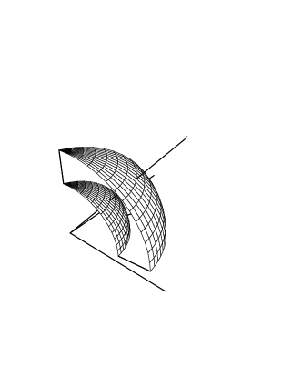
Figure 4: A fundamental region for the Eucidean black hole in the upper half-space representation is obtained by identifying the inner and outer hemispheres along radial lines such as $L$.

For the Euclidean black hole, the $\hbox{SL}(2,{\hbox{{\rm I}\kern-1.99997pt\hbox{\rm R}}})\!\times\!\hbox{SL}(2,{\hbox{{\rm I}\kern-1.99997pt\hbox{\rm R}}})$ holonomy of equation (2.68) is analytically continued to become an $\hbox{SL}(2,{\ \hbox{{\rm I}\kern-6.00006pt\hbox{\bf C}}})$ holonomy,

$$\rho[\gamma]=\left(\begin{array}[]{cc}e^{\pi(r_{+}+i|r_{-}|)/\ell}&0\\ 0&e^{-\pi(r_{+}+i|r_{-}|)/\ell}\end{array}\right).$$ (4.4)

On the other hand, if we consider a segment $\delta$ connecting the points $(R_{1},\theta_{1})$ and $(R_{2}=e^{\Sigma}R_{1},\theta_{2}=\theta_{1}+\Theta)$ along a surface of constant “radius” $\chi$, we find a holonomy

$$\rho[\delta]=\left(\begin{array}[]{cc}e^{\pi(\Sigma+i\Theta)/\ell}&0\\ 0&e^{-\pi(\Sigma+i\Theta)/\ell}\end{array}\right).$$ (4.5)

The Poisson brackets of the Chern-Simons theory then give brackets

$$\left\{r_{+},\Theta\right\} = \left\{|r_{-}|,\Sigma\right\}=4G$$

$$\left\{|r_{-}|,\Theta\right\} = \left\{r_{+},\Sigma\right\}=0,$$ (4.6)

providing us with a starting point for quantization.

What is the significance of the new parameters $\Theta$ and $\Sigma$? Recall that the Euclidean black hole metric is periodic in imaginary time, and that this periodicity determines the Hawking temperature. In the upper half-plane coordinates of (4.1), imaginary Schwarzschild time becomes to the “spherical” coordinate $\theta$, and periodicity requires identifying the two endpoints of the segment $\delta$. The resulting metric may be shown to be smooth at the horizon only if $\Sigma\!=\!0$ and $\Theta\!=\!2\pi$. Other values of these parameters correspond to Euclidean black holes with conical singularities at the horizon; as shown in [90], $2\pi-\Theta$ is a deficit angle, while $\Sigma$ represents a “helical twist.” Historically, this analysis of the three-dimensional black hole was the starting point for the observation [159] that conical singularities at the horizon may play an important role in black hole thermodynamics in arbitrary dimensions.

There is another, potentially even more powerful, way to employ the (2+1)-dimensional black hole to gain insight into black hole thermodynamics. In the Euclidean model discussed above, the horizon shrinks to a circle ($x\!=\!y\!=0$ in the coordinates (4.1)), and the conical singularity must encode its full dynamics. One may instead begin with the Lorentzian black hole and search directly for horizon dynamics that might provide a “microscopic” basis for black hole thermodynamics.

At first sight, this seems an unlikely prospect: as I have stressed throughout these lectures, (2+1)-dimensional gravity is characterized by a small number of global degrees of freedom, and there seems to be no room for “statistical mechanics.” Chern-Simons theories have a very peculiar feature, however: a Chern-Simons theory on a manifold $M$ with boundary can induce a dynamical Wess-Zumino-Witten theory, with an infinite number of degrees of freedom, on the boundary $\partial M$ [160, 161]. This phenomenon occurs because the presence of a boundary breaks the gauge symmetry, allowing would-be “pure gauge” degrees of freedom to become dynamical. It may therefore make sense to look at the event horizon of a black hole as a boundary, as suggested by the idea of “black hole complementarity” [162, 163], and investigate the induced WZW theory.

This program was begun in reference [69]. Starting with the Chern-Simons action (2.21) and boundary conditions corresponding to the presence of an apparent horizon, it is easy to find the induced $\hbox{SL}(2,{\hbox{{\rm I}\kern-1.99997pt\hbox{\rm R}}})\!\times\!\hbox{SL}(2,{\hbox{{\rm I}\kern-1.99997pt\hbox{\rm R}}})$ WZW action. This model is not completely understood, but in the large $k$—i.e., small $\Lambda$—limit, it may be approximated as a theory of six independent bosonic string oscillators. Such a system has an infinite number of states, but a remaining gauge invariance reduces these to a finite number of physical states. With plausible (although by no means certain) assumptions about the relevant boundary conditions and representations of operator algebras, these states can be counted; their number behaves asymptotically as

$$\log n(r_{+})\sim{2\pi r_{+}\over 4G},$$ (4.7)

giving precisely the right expression for the entropy of the (2+1)-dimensional black hole [86, 90]. Important uncertainties remain, but (2+1)-dimensional gravity may be offering a first glimpse into the quantum gravitational dynamics responsible for black hole thermodynamics.

4.2 Topology-Changing Amplitudes

Let me conclude with one more topic, the question of whether quantum gravity allows changes in the topology of space. Classically, it may be shown that topology-changing processes are forbidden [164], but there has long been speculation that quantum mechanical tunneling between spatial topologies may be allowed.

The natural way to approach such a question is by means of a path integral [9]. As discussed in subsection 3.4, path integrals in (2+1)-dimensional gravity may be computed exactly, yielding topological invariants such as Reidemeister torsion. To compute a topology-changing amplitude, we choose a manifold $M$ whose boundary

$$\partial M=\Sigma_{1}\amalg\Sigma_{2}$$ (4.8)

is the disjoint union of an “initial” surface $\Sigma_{1}$ and a “final” surface $\Sigma_{2}$, and we specify an induced spin connection $\tilde{\omega}$ on $\partial M$ as boundary data. We must then consider path integrals of the form

$$Z_{M}[\tilde{\omega}]=\int[d\omega][de]\,\exp\left\{iI_{\hbox{\scriptsize grav}}[M]\right\},$$ (4.9)

where $I_{\hbox{\scriptsize grav}}$ is the first-order action (2.10). Amano and Higuchi have shown that the requirement that the boundaries of $M$ be spacelike leads to “topological selection rules,” essentially requiring that the Euler characteristics of the initial and final spatial slices be equal [165]. These rules prevent a transition from a connected surface of genus $g$ to one of genus $g^{\prime}\!\neq\!g$. Since $\Sigma_{1}$ and $\Sigma_{2}$ may each have many connected components, however, this restriction still leaves room for a good deal of topology change.

The evaluation of the path integral (4.9) requires a careful analysis of the zero-modes of $e$ and $\omega$, whose number depends delicately on the boundary conditions. Such an analysis has been carried out in reference [145]. As Witten first pointed out, one will typically find infrared divergences coming from integrals over zero-modes of $e$; these essentially correspond to integrals over arbitrary lengths of closed curves in $M$, that is, “large universes.” Up to the problem of regulating these divergences, however, the computation may be carried out explicitly for simple topologies. Reference [145], for example, includes a computation of the amplitude for a genus 3 space to split into two disconnected genus 2 pieces. The possibility of performing such an exact computation is certainly peculiar to 2+1 dimensions, but this simple model at least shows that topology change is not forbidden by any fundamental principles. On the other hand, canonical quantum gravity on a manifold ${\hbox{{\rm I}\kern-1.99997pt\hbox{\rm R}}}\!\times\!\Sigma$, with no topology change, is also consistent, so it appears that some choices are available.

5. Conclusion

Spacetime is not three-dimensional, and (2+1)-dimensional gravity is clearly not a physically realistic model of our universe. Nevertheless, I hope I have convinced you that this simple model is rich enough to allow us to learn a good deal about the nature of quantum gravity. In particular, the method of covariant canonical quantization, with the approach to observables described in subsection 3.3, seems to offer a promising approach to some of the basic conceptual problems of quantum gravity. Moreover, the analyses of black hole thermodynamics and topology change may offer genuine physical insight into the real (3+1)-dimensional world.

Needless to say, there remains a great deal to be learned from this model. Of special interest is the problem of coupling matter to quantum gravity. There is an old suggestion that nonperturbative quantum gravitational effects might cut off the divergences of ordinary quantum field theories [166, 167, 168]. Ashtekar and Varadarajan have recently found evidence for this conjecture in 2+1 dimensions, in the form of an observation that the Hamiltonian of a scalar field coupled to (2+1)-dimensional gravity is bounded above [29]. Another interesting observation, due to Witten [169, 170], is that in the presence of gravity in 2+1 dimensions, unbroken supersymmetry may lead to a vanishing cosmological constant without requiring the equality of boson and fermion masses. For researchers in this field, much interesting work remains.

Acknowledgements

This work was supported in part by National Science Foundation grant PHY-93-57203 and Department of Energy grant DE-FG03-91ER40674.

References

- [1] A. Staruszkiewicz, Acta Phys. Polon. 24 (1963) 734.
- [2] H. Leutwyler, Nuovo Cimento 42A (1966) 159.
- [3] P. Collas, Am. J. Phys. 45 (1977) 833.
- [4] G. Clément, Nucl. Phys. B114 (1976) 437.
- [5] S. Deser, R. Jackiw, and G. ’t Hooft, Ann. Phys. 152 (1984) 220.
- [6] S. Deser and R. Jackiw, Commun. Math. Phys. 118 (1988) 495.
- [7] G. ’t Hooft, Commun. Math. Phys. 117 (1988) 685.
- [8] E. Witten, Nucl. Phys. B311 (1988) 46.
- [9] E. Witten, Nucl. Phys. B323 (1989) 113.
- [10] E. Witten, Commun. Math. Phys. 137 (1991) 29.
- [11] A. Achúcarro and P. K. Townsend, Phys. Lett. B180 (1986) 89.
- [12] J. R. Gott, Phys. Rev. Lett. 66 (1991) 1126.
- [13] S. M. Carroll et al., Phys. Rev. D50 (1994) 6190.
- [14] G. ’t Hooft, Class. Quant. Grav. 9 (1992) 1335.
- [15] P. Menotti and D. Seminara, Nucl. Phys. B419 (1994) 189.
- [16] R. Jackiw, in Proc. of the Sixth Marcel Grossmann Meeting on General Relativity, edited by H. Sato and T. Nakamura (World Scientific, Singapore, 1992).
- [17] M. Roček and R. M. Williams, Class. Quant. Grav. 2 (1985) 701.
- [18] G. Clément, Int. J. Theor. Phys. 24 (1985) 267.
- [19] P. Gerbert and R. Jackiw, Commun. Math. Phys. 124 (1989) 229.
- [20] S. Carlip, Nucl. Phys. B324 (1989) 106.
- [21] K. Koehler et al., Nucl. Phys. B348 (1991) 373.
- [22] S. Carlip, Class. Quant. Grav. 8 (1991) 5.
- [23] C. Vaz and L. Witten, Mod. Phys. Lett. A7 (1992) 2763.
- [24] M. K. Falbo-Kenkel and F. Mansouri, J. Math. Phys. 34 (1993) 139.
- [25] D. Kabat and M. E. Ortiz, Phys. Rev. D49 (1994) 1684.
- [26] J. Gegenberg, G. Kunstatter, and H. P. Leivo, Phys. Lett. B252 (1990) 381.
- [27] S. Carlip and J. Gegenberg, Phys. Rev. D44 (1991) 424.
- [28] S. Mizoguchi and H. Yamamoto, Phys. Rev. D50 (1994) 7351.
- [29] A. Ashtekar and M. Varadarajan, Phys. Rev. D50 (1994) 4944.
- [30] P. Peldan, Nucl. Phys. B395 (1993) 239.
- [31] G. Bonacina, A. Gamba, and M. Martellini, Phys. Rev. D45 (1992) 3577.
- [32] O. F. Dayi, Phys. Lett. B234 (1990) 25.
- [33] K. Koehler et al., J. Math. Phys. 32 (1991) 239.
- [34] D. de Wit, H. J. Matschull, and H. Nicolai, Phys. Lett. B318 (1993) 115.
- [35] H. J. Matschull and H. Nicolai, Nucl. Phys. B411 (1994) 609.
- [36] M. Henneaux, Phys. Rev. D29 (1984) 2766.
- [37] S. Deser, Class. Quant. Grav. 2 (1985) 489.
- [38] J. D. Brown, Lower Dimensional Gravity (World Scientific, Singapore, 1988).
- [39] P. Menotti and D. Seminara, Ann. Phys. 208 (1991) 449.
- [40] P. Menotti and D. Seminara, Nucl. Phys. B376 (1992) 411.
- [41] S. Deser, R. Jackiw, and S. Templeton, Ann. Phys. 140 (1982) 372.
- [42] S. Deser and Z. Yang, Class. Quant. Grav. 7 (1990) 1603.
- [43] B. Keszthelyi and G. Kleppe, Phys. Lett. B281 (1992) 33.
- [44] G. Grignani and G. Nardelli, Phys. Lett. B264 (1991) 45.
- [45] G. Grignani and G. Nardelli, Nucl. Phys. B370 (1992) 491.
- [46] T. Kawai, Phys. Rev. D49 (1994) 2862.
- [47] R. Brooks, Mod. Phys. Lett. A8 (1993) 2277.
- [48] R. Brooks and G. Lifschytz, “Quantum Gravity and Equivariant Cohomology,” MIT preprint MIT-CTP-2340 (1994).
- [49] W. Abikoff, The Real Analytic Theory of Teichmüller Space, Lecture Notes in Mathematics 820 (Springer-Verlag, Berlin, 1980).
- [50] A. Fischer and A. Tromba, Math. Ann. 267 (1984) 311.
- [51] For a nice introduction, see L. Keen, Math. Intelligencer 16 (1994) 11.
- [52] W. P. Thurston, The Geometry and Topology of Three-Manifolds, Princeton lecture notes (1979).
- [53] R. D. Canary, D. B. A. Epstein, and P. Green, in Analytical and Geometric Aspects of Hyperbolic Space, London Math. Soc. Lecture Notes Series 111, edited by D. B. Epstein (Cambridge University Press, Cambridge, 1987).
- [54] W. M. Goldman, in Geometry of Group Representations, edited by W. M. Goldman and A. R. Magid (American Mathematical Society, Providence, 1988).
- [55] For examples of geometric structures, see D. Sullivan and W. Thurston, Enseign. Math. 29 (1983) 15.
- [56] S. Carlip, in Knots and Quantum Gravity, edited by J. Baez (Clarendon Press, Oxford, 1994).
- [57] G. Mess, “Lorentz Spacetimes of Constant Curvature,” Institut des Hautes Etudes Scientifiques preprint IHES/M/90/28 (1990).
- [58] Y. Fujiwara, Class. Quant. Grav. 10 (1993) 219.
- [59] K. Ezawa, Phys. Rev. D49 (1994) 5211; addendum in Phys. Rev. D50 (1994) 2935.
- [60] J. D. Romano, Gen. Rel. Grav. 25 (1993) 759.
- [61] M. Bañados, “Sugawara Construction and the Relation between Diffeomorphisms and Gauge Transformations in General Relativity,” Imperial College preprint Imperial-TP-93-94-40 (1994).
- [62] E. Witten, Commun. Math. Phys. 121 (1989) 351.
- [63] J. E. Nelson and T. Regge, Nucl. Phys. B328 (1989) 190.
- [64] J. E. Nelson and T. Regge, Class. Quant. Grav. 9 (1992) 187.
- [65] J. E. Nelson and T. Regge, Phys. Lett. B272 (1991) 213.
- [66] S. Martin, Nucl. Phys. B327 (1989) 178.
- [67] R. Loll, “Wilson Loop Coordinates for 2+1 Gravity,” Penn State preprint CGPG-94-8-1 (1994).
- [68] J. E. Nelson, T. Regge, and F. Zertuche, Nucl. Phys. B339 (1990) 516.
- [69] S. Carlip, Phys. Rev. D51 (1995) 632.
- [70] W. M. Goldman, Adv. Math. 54 (1984) 200.
- [71] W. M. Goldman, Invent. Math. 85 (1986) 263.
- [72] V. Moncrief, J. Math. Phys. 30 (1989) 2907.
- [73] A. Hosoya and K. Nakao, Class. Quant. Grav. 7 (1990) 163.
- [74] J. W. York, Phys. Rev. Lett. 28 (1972) 1082.
- [75] A. M. Macbeath and D. Singerman, Proc. London Math. Soc. 31 (1975) 211.
- [76] W. M. Goldman, in Geometry and Topology, Lecture Notes in Mathematics 1167, edited by J. Alexander and J. Harer (Springer, Berlin, 1985).
- [77] W. M. Goldman, Invent. Math. 93 (1988) 557.
- [78] J. S. Birman and H. M. Hilden, in Advances in the Theory of Riemann Surfaces, Annals of Math. Studies 66, edited by L. V. Ahlfors et al. (Princeton University Press, Princeton, 1971).
- [79] J. S. Birman, in Discrete Groups and Automorphic Functions, edited by W. J. Harvey (Academic Press, New York, 1977).
- [80] S. Carlip and J. E. Nelson, “Comparative Quantizations of (2+1)-Dimensional Gravity,” Davis preprint UCD-94-37 and Torino preprint DFTT/49/94 (1994), to appear in Phys. Rev. D.
- [81] S. Carlip and J. E. Nelson, Phys. Lett. B324 (1994) 299.
- [82] K. Ezawa, “Chern-Simons Quantization of (2+1) Anti-de Sitter Gravity on a Torus,” Osaka preprint OU-HET/201 (1994).
- [83] J. Louko and D. M. Marolf, Class. Quant. Grav. 11 (1994) 311.
- [84] S. Carlip, Phys. Rev. D42 (1990) 2647.
- [85] Y. Fujiwara and J. Soda, Prog. Theor. Phys. 83 (1990) 733.
- [86] M. Bañados, C. Teitelboim, and J. Zanelli, Phys. Rev. Lett. 69 (1992) 1849.
- [87] M. Bañados, M. Henneaux, C. Teitelboim, and J. Zanelli, Phys. Rev. D48 (1993) 1506.
- [88] S. Carlip and A. Hosoya, in preparation.
- [89] J. D. Brown, J. Creighton and R. B. Mann, Phys. Rev. D50 (1994) 6394.
- [90] S. Carlip and C. Teitelboim, Phys. Rev. D51 (1995) 622.
- [91] D. Cangemi, M. Leblanc, and R. B. Mann, Phys. Rev. D48 (1993) 3606.
- [92] A. Hosoya and K. Nakao, Prog. Theor. Phys. 84 (1990) 739.
- [93] R. S. Puzio, Class. Quant. Grav. 11 (1994) 2667.
- [94] See, for example, H. Iwaniec, in Modular Forms, edited by R. A. Rankin (Ellis Horwood Ltd., Chichester, 1984).
- [95] R. Puzio, Class. Quant. Grav. 11 (1994) 609.
- [96] J. D. Fay, J. Reine Angew. Math. 293 (1977) 143.
- [97] H. Maass, Lectures on Modular Functions of One Complex Variable (Tata Institute, Bombay, 1964).
- [98] S. Carlip, Phys. Rev. D45 (1992) 3584.
- [99] S. Carlip, Phys. Rev. D47 (1993) 4520.
- [100] J. Isenberg and J. E. Marsden, Phys. Reports 89 (1982) 179.
- [101] K. Kuchař, in Proc. of the 4th Canadian Conf. on General Relativity and Relativistic Astrophysics, edited by G. Kunstatter et al. (World Scientific, Singapore, 1992).
- [102] J. E. Nelson and T. Regge, Commun. Math. Phys. 141 (1991) 211.
- [103] J. E. Nelson and T. Regge, Commun. Math. Phys. 155 (1993) 561.
- [104] J. E. Nelson and T. Regge, Phys. Rev. D50 (1994) 5125.
- [105] C. Rovelli, Phys. Rev. D42 (1990) 2638.
- [106] C. Rovelli, Phys. Rev. D43 (1991) 442.
- [107] A. Ashtekar and A. Magnon, Proc. Roy. Soc. (London) A346 (1975) 375.
- [108] C. Crnkovic and E. Witten, in Three Hundred Years of Gravity, edited by S. W. Hawking and W. Israel (Cambridge University Press, Cambridge, 1987).
- [109] A. Ashtekar. L. Bombelli, and O. Reula, in Mechanics, Analysis and Geometry: 200 Years after Lagrange, edited by M. Francaviglia (Elsevier Science Publishers, Amsterdam, 1991).
- [110] R. M. Wald, Quantum Field Theory in Curved Spacetime and Black Hole Thermodynamics (University of Chicago Press, Chicago, 1994).
- [111] See, for example, C. J. Isham, in Quantum Gravity, edited by C. J. Isham, R. Penrose, and D. W. Sciama (Clarendon Press, Oxford, 1975).
- [112] K. Ezawa, Int. J. Mod. Phys. A9 (1994) 4727.
- [113] P. Peldan, “Large Diffeomorphisms in (2+1) Quantum Gravity on the Torus,” Penn State preprint CGPG-95-1-1 (1995).
- [114] S. Carlip, in Proc. of the Fifth Canadian Conference on General Relativity and Relativistic Astrophysics, edited by R. B. Mann and R. G. McLenaghan (World Scientific, Singapore, 1994).
- [115] S. Carlip, Class. Quant. Grav. 11 (1994) 31.
- [116] M. Henneaux, Phys. Lett. B134 (1984) 184.
- [117] M. Visser, Phys. Rev. D42 (1990) 1964.
- [118] T. Banks, W. Fischler, and L. Susskind, Nucl. Phys. B262 (1985) 159.
- [119] A. Ashtekar, Lectures on Nonperturbative Quantum Gravity (World Scientific, Singapore, 1991).
- [120] A. Ashtekar et al., Class. Quant. Grav. 6 (1989) L185.
- [121] C. Rovelli and L. Smolin, Nucl. Phys. B331 (1990) 80.
- [122] D. Marolf, Class. Quant. Grav. 10 (1993) 2625.
- [123] L. Smolin, in Knots, Topology, and Quantum Field Theories, edited by L. Lusanna (World Scientific, Singapore, 1989).
- [124] A. Ashtekar and R. Loll, Class. Quant. Grav. 11 (1994) 2417.
- [125] H. Waelbroeck, Class. Quant. Grav. 7 (1990) 751.
- [126] H. Waelbroeck, Phys. Rev. Lett. 64 (1990) 2222.
- [127] H. Waelbroeck and F. Zertuche, Phys. Rev. D50 (1994) 4966.
- [128] G. ’t Hooft, Class. Quant. Grav. 10 (1993) S79.
- [129] W. G. Unruh and P. Newbury, Int. J. Mod. Phys. D3 (1994) 131.
- [130] G. Ponzano and T. Regge, in Spectroscopic and Group Theoretical Methods in Physics, edited by F. Block (North-Holland, Amsterdam, 1968).
- [131] B. Hasslacher and M. J. Perry, Phys. Lett. B103 (1981) 21.
- [132] V. G. Turaev and O. Y. Viro, Topology 31 (1992) 865.
- [133] H. Ooguri and N. Sasakura, Mod. Phys. Lett. A6 (1991) 3591.
- [134] H. Ooguri, Nucl. Phys. B382 (1992) 276.
- [135] F. Archer and R. M. Williams, Phys. Lett. B273 (1991) 438.
- [136] C. Rovelli, Phys. Rev. D48 (1993) 2702.
- [137] J. Iwasaki, “A Reformulation of the Ponzano-Regge Quantum Gravity Model in Terms of Surfaces,” Pittsburgh preprint (1994).
- [138] T. J. Foxon, “Spin Networks, Turaev-Viro Theory and the Loop Representation,” Cambridge preprint DAMTP-R-94-30 (1994).
- [139] J. W. Barrett and T. J. Foxon, Class. Quant. Grav. 11 (1994) 543.
- [140] D. B. Ray and I. M. Singer, Adv. Math. 7 (1971) 145.
- [141] J. W. Milnor, Bull. Amer. Math. Soc. 72 (1966) 358.
- [142] W. Lück, J. Diff. Geom. 37 (1993) 263.
- [143] J. Gegenberg and G. Kunstatter, Ann. Phys. 231 (1994) 270.
- [144] G. Gonzalez and J. Pullin, Phys. Rev. D42 (1990) 3395.
- [145] S. Carlip and R. Cosgrove, J. Math. Phys. 35 (1994) 5477.
- [146] Y. Fujiwara et al., Phys. Rev. D44 (1991) 1756.
- [147] Y. Fujiwara et al., Phys. Rev. D44 (1991) 1763.
- [148] Y. Fujiwara et al., Class. Quant. Grav. 9 (1992) 867.
- [149] S. Carlip, Phys. Rev. D46 (1992) 4387.
- [150] S. Carlip, Class. Quant. Grav. 10 (1993) 207.
- [151] S. Carlip and S. P. de Alwis, Nucl. Phys. B337 (1990) 681.
- [152] S. Mizoguchi, Mod. Phys. Lett. A8 (1993) 3909.
- [153] E. Martinec, Phys. Rev. D30 (1984) 1198.
- [154] P. O. Mazur, Phys. Lett. B262 (1991) 405.
- [155] S. W. Hawking, Nature 248 (1974) 30.
- [156] M. Bañados, C. Teitelboim, and J. Zanelli, Phys. Rev. Lett. 72 (1994) 957.
- [157] J. Louko and B. F. Whiting, “Hamiltonian Thermodynamics of the Schwarzschild Black Hole,” Florida preprint UF-RAP-94-13 (1994).
- [158] See, for example, T. Banks, in The Santa Fe TASI-87, edited by R. Slansky and G. West (World Scientific, Singapore, 1988).
- [159] S. Carlip and C. Teitelboim, “The Off-Shell Black Hole,” IAS preprint IASSNS-HEP-93/84 and Davis preprint UCD-93-34 (1993).
- [160] G. Moore and N. Seiberg, Phys. Lett. B220 (1989) 422.
- [161] S. Elitzur et al., Nucl. Phys. B326 (1989) 108.
- [162] L. Susskind, L. Thorlacius, and J. Uglum, Phys. Rev. D48 (1993) 3743.
- [163] M. Maggiore, Phys. Lett. B333 (1994) 39.
- [164] R. P. Geroch, J. Math. Phys. 8 (1967) 782.
- [165] K. Amano and S. Higuchi, Nucl. Phys. B377 (1992) 218.
- [166] B. S. DeWitt, Phys. Rev. Lett. 13 (1964) 114.
- [167] C. J. Isham, A. Salam, and J. Strathdee, Phys. Rev. D3 (1971) 1805.
- [168] C. J. Isham, A. Salam, and J. Strathdee, Phys. Rev. D5 (1972) 2548.
- [169] E. Witten, “Is Supersymmetry Really Broken?” IAS preprint IASSNS-HEP-94-72 (1994).
- [170] K. Becker, M. Becker, and A. Strominger, “Three-Dimensional Supergravity and the Cosmological Constant,” Santa Barbara ITP preprint NSF-ITP-95-07 (1995).