MIT-CTP-2384

TUTP-94-22

gr-qc/9412040

November 1994

A Note on the Semi-Classical Approximation
in Quantum Gravity^∗

Gilad Lifschytz, Samir D. Mathur Center for Theoretical Physics, Laboratory for Nuclear Science
and Department of Physics,
Massachusetts Institute of Technology, Cambridge MA 02139, USA.
e-mail: gil1 or mathur @mitlns.mit.edu and Miguel Ortiz Institute of Cosmology, Department of Physics and Astronomy,
Tufts University, Medford, MA 02155, USA.
e-mail: mortiz@tufts.edu

Abstract: We re-examine the semiclassical approximation for quantum gravity in the canonical formulation, focusing on the definition of a quasiclassical state for the gravitational field. It is shown that a state with classical correlations must be a superposition of states of the form $e^{iS}$. In terms of a reduced phase space formalism, this type of state can be expressed as a coherent superposition of eigenstates of operators that commute with the constraints and so correspond to constants of the motion. Contact is made with the usual semiclassical approximation by showing that a superposition of this kind can be approximated by a WKB state with an appropriately localised prefactor. A qualitative analysis is given of the effects of geometry fluctuations, and the possibility of a breakdown of the semiclassical approximation due to interference between neighbouring classical trajectories is discussed. It is shown that a breakdown in the semiclassical approximation can be a coordinate dependent phenomenon, as has been argued to be the case close to a black hole horizon.

^∗ This work was supported in part by funds provided by the U.S. Department of Energy (D.O.E.) under cooperative agreement DE-FC02-94ER40818, and in part by the National Science Foundation.

1 Introduction

Although we have few clues about the final form of a quantum theory of gravity, there is at least one constraint that we can be sure of: That the theory should, in some limit, describe quantum matter fields interacting with an essentially classical background spacetime in what is known as the semiclassical limit of quantum gravity. In some formulations of quantum gravity, such as perturbation theory around a fixed background, the semiclassical limit is guaranteed. However, at a more fundamental level we expect the notion of spacetime to be a derived concept. In any theory reflecting this feature, it is interesting to understand how the notion of a classical background emerges.

Some considerable work towards understanding the semiclassical limit has been done in the canonical approach to quantum gravity using the ADM formulation [1]. In this approach there is no background spacetime, since the dynamical variables are the 3-metrics of spacelike hypersurfaces, plus the matter fields on these hypersurfaces. Employing the Dirac procedure, physical states must be annihilated by the momentum and Hamiltonian constraints. The momentum constraints reduce the configuration space to the space of all 3-geometries (the equivalence classes of 3-metrics under spatial diffeomorphisms). The Hamiltonian constraint is imposed by the Wheeler–DeWitt equation

$${\cal H}\Psi[h,\phi]=0$$ (1)

which has the effect of factoring out translations in the time direction, and is a direct analogue of the Klein-Gordon equation for the quantized relativistic particle.

The semiclassical limit is obtained by expanding the Wheeler–DeWitt equation in powers of the gravitational coupling constant $G$. This really involves two separate approximations: A WKB approximation (effectively in $\hbar$) in the gravitational (or more generally classical) sector, and a Born-Oppenheimer approximation separating the gravity and matter (classical and quantum) parts. At each order, one performs first the gravitational WKB approximation, and then solves the remaining equation for the matter state. In this way the complete solution of the Wheeler–DeWitt equation is split into a product of a purely gravitational piece representing the classical geometry and a mixed piece representing quantum field theory on that background (for simplicity we shall assume that the gravitational field is the only classical variable).

To first order, the expansion of the Wheeler–DeWitt equation yields the first WKB approximation

$$\Psi[h,\phi]=e^{iS_{HJ}[h_{ij}]/\hbar G},\qquad{1\over 2}G_{ijkl}{\delta S_{HJ}\over\delta h_{ij}}{\delta S_{HJ}\over\delta h_{kl}}-2\sqrt{h}R=0$$ (2)

to the gravitational Wheeler–DeWitt equation, where $S_{HJ}[h_{ij}]$ is a Hamilton–Jacobi functional for general relativity. We shall refer to a state of this form, without a prefactor, as a first order WKB state. This first order approximation depends only on the gravitational degrees of freedom.

Any functional $S_{HJ}[h_{ij}]$ that solves the Hamilton–Jacobi equation defines a congruence of classical trajectories in superspace, made up of all possible foliations of all solutions of Einstein’s equations defined by $S_{HJ}$ (see Fig. 1).

As was shown by Lapchinski and Rubakov, and later by Banks [2, 3], the next order approximation is obtained by solving two equations: An equation for the gravitational WKB prefactor $D[h]$, and a functional differential equation for the remainder of the state $\chi[h,f]$ that depends on the matter variables $f$. Solving the equation for $\chi[h,f]$ is equivalent to solving the functional Schrödinger equation along each of the congruence of eikonal trajectories corresponding to the set of all foliations of all solutions of Einstein’s equations given by $S_{HJ}[h_{ij}]$.

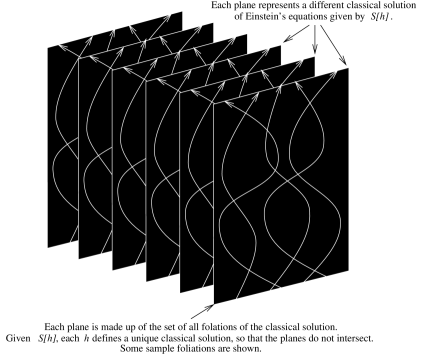
Figure 1: A congruence of classical solutions in superspace. Each classical solution is shown as a plane in the diagram, which contains the different trajectories in superspace corresponding to that solution, given by different choices of the lapse and shift functions.

The semiclassical approximation to second order should yield a state that represents a quantum matter field propagating on a quasiclassical background spacetime. The results we have described are not quite the whole story, since they do not in themselves provide a complete description of such a quantum state. A careful treatment of the gravitational degrees of freedom is needed in order to restrict the semiclassical approximation to the propagation of quantum matter fields on a single background.

A semiclassical state with a gravitational WKB part that defines a congruence of classical trajectories on superspace is not suitable for describing classical behaviour. In Ref. [4], an approximate form of the Wigner function was used to argue that a generic first order gravitational WKB state has classical correlations between coordinates and momenta. However, it was later pointed out in a simple example that the exact Wigner function of a general WKB state does not exhibit such correlations [5, 6], unless a particular form of the WKB prefactor is chosen, corresponding to a coherent superposition of first order WKB states. These results are analogous to the simple statement in quantum mechanics that a plane wave does not exhibit classical correlations, but that plane wave states may be superposed to construct a coherent state.

1.1 An Outline

We shall argue in this paper that in quantum gravity, a quasiclassical state should be a ‘coherent state’ in an appropriately defined sense: The uncertainty of a complete set of spacetime diffeomorphism invariant operators (constants of the motion) should be small (a similar proposal was made some years ago Komar [7]). We shall show that this condition, although somewhat formal, can be realised in a concrete way. Since the classical counterparts of the diffeomorphism invariants together specify a unique classical solution, this point of view reinforces the notion that a classical state in quantum gravity gives rise to only an approximate background spacetime. We shall go on to argue that a coherent state can and must be used as the gravitational state providing a background for the semiclassical approximation. The approximate nature of the background described by such a state will be shown to determine some limits of the semiclassical approximation.

The Hamilton–Jacobi formalism can be used to define a natural complete set of diffeomorphism invariant operators. Through the Hamilton–Jacobi formalism, we shall show that a first order WKB state approximates an eigenstate with respect to half of these operators (the $\alpha$’s of Hamilton–Jacobi theory). Given this simple observation it follows that a coherent or quasiclassical state is approximated by a coherent superposition of first order WKB states. The rewriting of our quasiclassical states in quantum gravity as coherent superpositions of first order WKB states makes direct contact with the work of Gerlach [8]. He observed that a superposition of WKB states can be arranged to have support only in a narrow ‘tube’ in superspace around 3-geometries comprising a solution of Einstein’s equations. This observation relates the metric-dependent and coordinate invariant notions of what constitutes a quasiclassical state. Gerlach’s interpretation seems to have fallen out of favour in recent years, but we hope to revive it in this paper.

The fact that a coherent state can be written in the WKB approximation using the metric representation is important for a second reason. It allows us to use the coherent state in the standard semiclassical approximation as described above. An important consequence of the connection between first order WKB states and $\alpha$ eigenstates is that the expectation value of conjugate operators (the $\beta$ operators of Hamilton–Jacobi theory) in such a state is maximally uncertain. Thus a first order WKB state cannot be expected to have a Wigner function with strong correlations between coordinates and momenta, and so is not appropriate for describing a background spacetime. However, a coherent state can be used as a background for the semiclassical approximation. It exhibits quasiclassical correlations and its WKB approximation is precisely a second order WKB state of the form

$$\Psi[h_{ij}]={1\over D[h_{ij}]}\,e^{iS_{HJ}[h_{ij}]}$$

with an appropriately chosen prefactor $D[h_{ij}]$. $D[h_{ij}]$ is given by rewriting the coherent superposition of first order WKB states as a second order WKB state. Using the language of Vilenkin [9], the WKB prefactor can be regarded as providing a measure on the space of all classical solutions compatible with $S_{HJ}[h_{ij}]$. A coherent superposition is simply a WKB state with this measure concentrated around a minimally narrow band of classical solutions which effectively represent a single classical spacetime (the width of such a band is determined by the condition that the prefactor be of second order in the WKB approximation, and thus not vary too rapidly).

After establishing the validity of the semiclassical approximation using a coherent quasiclassical state, we shall go on to discuss in the last part of the paper the situations that can lead to a breakdown of this approximation scheme. Normally, the breakdown of the semiclassical approximation is thought to be governed by the behaviour of matter fields on a fixed classical background, with large quantum fluctuations in the matter fields leading to a loss of classical behaviour. Even in more careful studies of corrections to the semiclassical approximation [13], the emphasis has been on corrections to the equation describing evolution along individual eikonal trajectories (the functional Schrödinger equation), rather than on interference between neighbouring trajectories.

The notion that a state in quantum gravity can at best describe a small neighbourhood of classical backgrounds indicates a simple limitation of the semiclassical approximation. Recall that the fact that macroscopically different eikonal trajectories in superspace (corresponding to different classical solutions) can lead to different matter evolution, underlies the notion of decoherence between different classical histories. This is commonly believed to provide a promising explanation of the emergence of our classical world. However, because any quasiclassical state describing the gravitational background has a finite spread, the mechanism responsible for decoherence can actually spoil classical behaviour [14]: If neighbouring geometries contained within the spread of a quasiclassical state lead to substantially different matter evolution, then the notion of quantum field theory on a fixed background breaks down. We shall discuss this aspect of the semiclassical approximation in the last section of this paper. It is of particular interest since it has recently been shown that problems of this kind spoil the semiclassical approximation close to a black hole horizon [15, 16, 17].

It is appropriate at this point to mention two caveats to our work. First of all, we shall not discuss the mechanisms by which one may arrive at the quasiclassical states described in this paper. Our emphasis is simply on describing states that could reasonably be called classical and should therefore arise naturally from initial conditions, decoherence or some similar mechanism explaining the emergence of classical configurations. For this reason, we shall also not discuss the possibility of superpositions or ensembles of quasiclassical states. We refer the reader to the extensive literature on quantum cosmology for an open ended discussion of some of these issues. Secondly, the approach we take compares and relates quantisation in the metric representation to that using the constants of the motion as the fundamental observables. One would hope that at some fundamental level these descriptions are equivalent. However, it should be pointed out that this equivalence is not yet understood. For example, It has been noted recently [10] that there can be more than one way of defining the Hilbert space in quantum gravity. More precisely, even though one knows the algebra of operators of a theory, the choice of what states are physical and what states are unphysical can be made in more than one way, thus giving inequivalent quantum theories. The resulting quantum theories are also likely to depend on the classical variables used as a starting point for quantisation. Nevertheless, a valuable tool in resolving ambiguities of this kind is to study the semiclassical limit of quantum gravity, since this gives definite information about the physical spectrum of the desired theory of quantum gravity. Although it is known that there are difficulties in operator ordering the Wheeler–DeWitt operator that block the construction of wavefunctionals [11, 12], any reasonable quantisation in a metric (or connection) representation should be equivalent to quantisation in terms of constants of the motion, at least in the semiclassical limit.

1.2 A simple example

Before beginning a discussion of WKB states in quantum gravity, it is useful to run through the definition of a quasiclassical state for the simple case of the relativistic particle. For the sake of extreme simplicity, we shall work with a massless particle in 1+1 dimensional flat spacetime. The unconstrained phase space for the particle consists of the spacetime coordinates $x^{\mu}$ and their conjugate momenta. Time translations are generated by the constraint $p^{2}=0$ so that physical states in the coordinate representation satisfy the Klein–Gordon equation

$$\hbar^{2}\partial^{\mu}\partial_{\mu}\psi(x^{\mu})=0$$ (3)

In this simple case, we know that the space of physical states is just the set of all functions $\psi^{+}(x^{+})+\psi^{-}(x^{-})$. However, let us try to find solutions in the WKB approximation. We write

$$\psi(x^{\mu})=e^{iS_{0}(x^{\mu})/\hbar+iS_{1}(x^{\mu})+i\hbar S_{2}(x^{\mu})+\ldots}$$ (4)

The first term in an expansion in powers of $\hbar$ yields the Hamilton–Jacobi equation

$$\hbar^{2}(\partial_{\mu}S_{0})(\partial^{\mu}S_{0})=0$$ (5)

for $S_{0}(x^{\mu})$, so that

$$\psi_{0}(x^{\mu};P,\pm)=e^{iS_{0}(x^{\mu};P,\pm)/\hbar}=e^{iP_{\mu}x^{\mu}/\hbar}=e^{iPx^{\pm}/\hbar}$$ (6)

is a first order WKB state. A solution of the Hamilton–Jacobi equation is given by any function of the form $S_{0}=P_{\mu}x^{\mu}=Px^{\pm}$, with $P_{\mu}=(P,\pm P)$ where $P$ and the choice of sign enter as simple constants of integration (we are ignoring an additive constant). $S_{0}$ then defines the congruence of trajectories with momentum $P_{\mu}$, since the Hamilton–Jacobi function assigns a momentum

$$p_{\mu}={\partial S(x^{\mu};P;\pm)\over\partial x^{\mu}}=P_{\mu}$$ (7)

at each spacetime point. For any value of $P$, $P_{\mu}=(P,P)$ defines the congruence of left moving trajectories with momentum $P$ and $P_{\mu}=(P,-P)$ the right-moving trajectories. By specifying a second constant

$$X={\partial S_{0}(x^{\mu};P,\pm)\over\partial P}=x^{\pm}$$ (8)

a particular trajectory is selected from the congruence (essentially by specifying the value of $x$ at $t=0$). Thus specifying a value for $P$ and $X$ completely specifies a classical solution. We may invert the relations (7) and (8) to obtain $X$ and $P$ as functions of $x^{\mu}$ and $p_{\mu}$. $X(x^{\mu},p_{\mu})$ and $P(x^{\mu},p_{\mu})$ are then constants of the motion. They thus have weakly vanishing Poisson brackets with the constraint $p^{2}=0$ . They are also conjugate operators with quantum commutators $\{X,P\}=1$.

The second order WKB state is obtained by solving the Klein–Gordon equation to order $\hbar$. From this it follows that

$$\partial_{\mu}S_{1}\partial^{\mu}S_{0}=0$$

so that $\partial_{\mp}S_{1}=0$. The imaginary part of $S_{1}$ becomes the WKB prefactor so that the second order WKB state is of the form

$$\psi(x^{\mu})={1\over D(x^{\mu})}e^{iS_{0}(x^{\mu})/\hbar}={1\over D(x^{\pm})}e^{iPx^{\pm}/\hbar}$$ (9)

where $D(x^{\mu})=e^{-iS_{1}(x^{\mu})}$, ignoring any lower order correction to $S_{0}$.

In order to get a state that is localised in both momentum and position, we simply construct the relativistic analogue of a coherent state in terms of the constants of the motion $X(x^{\mu},p_{\mu})$ and $P(x^{\mu},p_{\mu})$. These constants of the motion are precisely the functions of $x^{\mu}$ and $p_{\mu}$ that define classical behaviour. In order to define a coherent state, we must first introduce some scales into the problem. We can study a system with a given characteristic momentum and characteristic spacetime resolution whose product is much larger than $\hbar$. We can then define a Gaussian superposition of first order WKB states of the form

$$\psi(x^{\mu})={1\over(16\pi^{3}{\bar{P}}^{2}/\hbar\omega)^{1/4}}\int dPe^{-(P-{\bar{P}})^{2}/2\hbar\omega}e^{iP_{\mu}x^{\mu}/\hbar}e^{-i(P-{\bar{P}}){\bar{X}}/\hbar}$$ (10)

where the last term is a phase that fixes $X$ to be localised around ${\bar{X}}$, and $\omega$ indicates that the uncertainties in position and momentum need not be equal. There is only constructive interference between the oscillating functions when (8) is satisfied.

Performing the integral in (10) gives

$$\psi(x^{\mu})=\left({\hbar\omega\over 4\pi{\bar{P}}^{2}}\right)^{1/4}e^{-\omega(x^{0}\pm x^{1}-{\bar{X}})^{2}/2\hbar}e^{i{\bar{P}}_{\mu}x^{\mu}/\hbar}$$ (11)

This is exactly of the second order WKB form (9), with $S_{1}$ giving a prefactor that is a function of the combination $X=x^{0}\pm x^{1}$ (i.e. gives a measure on the congruence of trajectories with fixed $P$), and is in this sense localised around solutions with $X=\bar{X}$ as expected.

The Wigner function for the quasiclassical state (11) can be easily computed, and is equal to

$$F(x^{\mu},p_{\mu}) = \int du\psi^{*}(x^{\mu}-u^{\mu}/2)\psi(x^{\mu}+u^{\mu}/2)e^{-ip_{\mu}u^{\mu}/\hbar}$$ (12)

$$= \left({4\hbar^{3}\pi\over\omega}\right)^{1/2}e^{-\omega(x^{\pm}-\bar{X})^{2}/\hbar}e^{-({\bar{P}}-p_{0})^{2}/\hbar\omega}\delta(p_{0}\pm p_{1})$$ (13)

which is exactly of the form one expects for a left (right) moving classical particle, localised in momentum and in $x^{+}$ $(x^{-})$.

We could instead have worked directly in terms of eigenstates of the operators $X$ and $P$. For a massless particle, the first order WKB states are exact eigenstates of the operator $P$. A coherent superposition of such states is clearly localised in both $P$ and $X$ and in this sense is quasiclassical. It is easy to check (and follows from the superposition principle) that a state of this kind has support only on $x^{\mu}$ within a narrow tube around the trajectory defined by the mean values of $P$ and $X$.

We are now ready to begin a rudimentary discussion of quasiclassical states in quantum gravity. In section 2, we shall review the standard semiclassical approximation in quantum gravity, obtained by expanding the Wheeler–DeWitt equation in powers of the Planck mass, and show how the WKB approximation for the quantum gravitational degrees of freedom, and the functional Schrödinger equation for the matter degrees of freedom arise. In section 3, we shall discuss the application of the Hamilton–Jacobi formalism to the gravitational field. Much of this discussion is somewhat formal (at least in the context of an infinite number of degrees of freedom), but it is useful for understanding first order WKB states and their relation to gauge invariant quantization on the space of all classical solutions. An appendix contains some details of how the Hamilton–Jacobi formalism leads to the definition of gauge invariant operators in a 1+1 dimensional cosmological model. In section 4, we run through the three equivalent definitions of a quasiclassical state for the gravitational field – as a coherent state in terms of constants of the motion, as a superposition of first order WKB states, and as a second order WKB state with a localised prefactor – making use of some of the ideas discussed in section 3. It follows directly from the last definition that the usual semiclassical approximation applies for this gravitational state and yields the functional Schrödinger equation, but now effectively on a single background spacetime. Section 5 contains a discussion of corrections to the semiclassical approximation arising from an excessive sensitivity of the matter evolution to very small changes in the background spacetime.

2 The semiclassical approximation

Expanding the Wheeler–DeWitt and momentum constraint equations order by order in the gravitational coupling constant $G$ leads to what is now well known as the semiclassical approximation of quantum gravity. In this section, we shall give a brief review of some of the large amount of work on this subject (see [2, 3, 4, 9, 13, 18, 19] and references therein).

We shall ignore the details of the momentum constraint in the following discussion, and assume that spatial diffeomorphism invariance is imposed at all orders. We shall assume a compact spatial topology, although this discussion can be generalized to open spacetimes with well-defined asymptotics (see for example the Appendix).

The Wheeler-DeWitt equation reads

$$-16\pi G\hbar^{2}G_{ijkl}{\delta^{2}\Psi[f,h]\over\delta h_{ij}\delta h_{kl}}-{\sqrt{h}R\over 16\pi G}\Psi[f,h]+{\cal H}_{matter}\Psi[f,h]=0$$ (14)

taking $c=1$. Consider expanding the state $\Psi$ as

$$\Psi=e^{i(S_{0}/G+S_{1}+GS_{2}+\cdots)/\hbar}$$ (15)

where each $S_{i}$ is assumed to be of the same order. Eq. (14) can then be expanded perturbatively in $G$. The zeroth order equation (order $1/G^{2}$) simply states that $S_{0}[f,h]=S_{0}[h]$ is independent of the matter degrees of freedom. At the first non-trivial order (order $1/G$), we find that $S_{0}[h]$ must be a solution of the general relativistic Hamilton–Jacobi equation [8, 20]

$${1\over 2}G_{ijkl}{\delta S_{0}\over\delta h_{ij}}{\delta S_{0}\over\delta h_{kl}}-2\sqrt{h}R=0.$$ (16)

There is a large freedom in specifying solutions of the Hamilton–Jacobi equation (16), since it is necessary to specify a set of integration constants. This is familiar from Hamilton–Jacobi theory, as we shall see in the next section.

At the next order, we obtain an equation for $S_{1}[f,h]$. It is convenient to split $S_{1}[f,h]$ into two functionals $\chi[f,h]$ and $D[h]$, where

$${1\over D[h]}e^{iS_{0}[h]/\hbar G}$$ (17)

is the second order WKB approximation to the purely gravitational Wheeler–DeWitt equation. The equation for the WKB prefactor $D[h]$ is

$$G_{ijkl}{\delta S_{0}[h]\over\delta h_{ij}}{\delta D[h]\over\delta h_{kl}}-{1\over 2}G_{ijkl}{\delta^{2}S_{0}[h]\over\delta h_{ij}\delta h_{kl}}D[h]=0.$$ (18)

The remaining condition on $\chi[f,h]$,

$$i\hbar G_{ijkl}{\delta S_{0}\over\delta h_{ij}}{\delta\chi[f,h]\over\delta h_{kl}}={\cal H}_{matter}\chi[f,h]$$ (19)

is an evolution equation for the functional $\chi[f,h]$ on the whole of superspace (the space of all 3-geometries), and as such, its solution requires initial data for $\chi[f,h]$ on a surface in superspace that is crossed once by each classical trajectory defined by $S_{0}[h_{ij}]$.

Let us now recall how Eq. (19) is closely related to the functional Schrödinger equation. Having specified the initial data, it can be solved by the method of characteristics along the eikonal tracks on superspace defined by $S_{0}$. These tracks are the integral curves of the Hamilton–Jacobi momenta, and are defined as solving the equations

$$\pi^{ij}=\delta S_{0}[h]/\delta h_{ij}\qquad{\rm or}\qquad{dh_{ij}({\bf x},\tau)\over d\tau}=-2N({\bf x},\tau)K_{ij}({\bf x},\tau)+\nabla_{(i}N_{j)}({\bf x},\tau)$$ (20)

These are the set of solutions of Einstein’s equations defined by the Hamilton–Jacobi functional $S_{0}[h]$. The solution of Eq. (20) requires a choice of integration constants and a choice of lapse and shift functions $N({\bf x},\tau)$ and $N_{i}({\bf x},\tau)$. The integration constants specify different classical solutions while the lapse and shift are just choices of coordinates on each of these spacetimes. Along each eikonal, Eq. (19) becomes the functional Schrödinger equation

$$i\hbar{\delta\chi[f,h]\over\delta\tau}=H_{matter}\chi[f,h]$$ (21)

where $\tau$ is the time parameter corresponding to the chosen foliation.

As an aside, we remark that there are two potential integrability conditions to worry about when solving Eq. (19) using the method of characteristics. Firstly, Eq. (20) can be integrated using different lapse and shift functions, corresponding to using different coordinates on the background spacetime. We expect (21) to be covariant under changes of coordinates, but this is not always the case. Integration with different lapse and shift functions can lead to ambiguities in the definition of $\chi[f,h]$, as has been discussed by various authors [21, 12, 22]. We shall ignore this problem here. Secondly, there is the question of different integration constants in the solution of Eq. (20), corresponding to integration of (19) along different classical spacetimes. To the present order this causes no problems, since in general there is at most one solution to Einstein’s equations that passes through any point in superspace and is compatible with a given Hamilton-Jacobi functional $S_{0}[h]$ (that is the eikonals never intersect). However, as we shall see in Sec. 5, evolution along neighbouring eikonals is an important issue when considering corrections to the semiclassical approximation.

It is possible to extend this approximate solution to the Wheeler–DeWitt equation beyond second order. At that point the semiclassical picture of field theory on a fixed background is lost. In principle, though, the approximation scheme can be continued, separating the higher order WKB approximations in the gravitational sector and corrections to the evolution equation in the matter sector [13]. A general understanding of these corrections is useful in determining the validity of the second order approximation.

Although it might seem that obtaining the functional Schrödinger equation is all there is to the semiclassical approximation, there is still the question of whether the construction described above really describes quantum field theory on a single spacetime. Since each eikonal trajectory defined by $S_{0}[h]$ is exactly classical, it does not make sense to regard a WKB state as describing an ensemble of independent classical solutions. Even if some form of decoherence is invoked, it is impossible for a quantum state to describe an ensemble of strictly classical spacetimes. To complete the semiclassical picture, we must understand the nature of the gravitational background provided by the gravitational WKB state.

3 Hamilton–Jacobi formalism in quantum gravity

Let us begin by considering the general relativistic Hamilton-Jacobi equation (16) (see Ref. [7]). In order to specify a solution of (16), it is necessary to supply a series of constants of integration which are usually called $\alpha$–parameters in Hamilton–Jacobi theory (see for example Ref. [23]). Any solution $S$ takes the form $S[h_{ij}(x);\alpha_{I}]$, where ${\alpha_{I}}$ represents an infinite number of integration constants (equivalent to two field theory degrees of freedom in 3+1 dimensions [19]), and so labels different solutions $S[h]$ of the Hamilton–Jacobi equation. Given a Hamilton–Jacobi functional $S[h;{\alpha_{I}}]$, the relation

$$\pi^{ij}={\delta S[h_{ij};{\alpha_{I}}]\over\delta h_{ij}}$$ (22)

gives the momenta conjugate to $h$ in terms of $h$ and ${\alpha_{I}}$. Eqs. (22), replacing $\pi^{ij}$ with $d{h}_{ij}/d\tau$ for some parameter $\tau$, are a set of first order differential equations (c.f. Eqs. (20)), that yield a congruence of solutions to Einstein’s equations, but require a further set of integration constants to pick out a particular solution. Equivalently, a classical solution can be fixed by defining the values of a set of functionals

$${\beta_{I}}={\delta S[h_{ij};{\alpha_{I}}]\over\delta{\alpha_{I}}},$$ (23)

which are precisely the integration constants for (22), and then solving for $h_{ij}$. The set of all $h_{ij}$ that satisfy this equation form sheaf of trajectories in superspace defining a solution of Einstein’s equations (in the same way that (8) specified a set of coordinates making up a classical trajectory). From either (22) or (23) it follows that a single solution of Einstein’s equations requires a choice of values for both the ${\alpha_{I}}$ and ${\beta_{I}}$ parameters. It also follows that given a set of ${\alpha_{I}}$ parameters (i.e. a Hamilton–Jacobi functional), a 3-geometry $h_{ij}$ fixes a unique value of ${\beta_{I}}$ for which the ${\alpha_{I}},{\beta_{I}}$ spacetime contains $h_{ij}$.

Eqs. (22) and (23) can be turned around to give a set of conjugate functionals ${\alpha_{I}}[h_{ij},\pi^{ij}]$ and ${\beta_{I}}[h_{ij},\pi^{ij}]$ which are constants of the motion – that is they have weakly vanishing Poisson bracket with the Hamiltonian constraint. These definitions provide a canonical transformation between the $h_{ij}({\bf x})$ and $\pi^{ij}({\bf x})$ and the ${\alpha_{I}}$ and ${\beta_{I}}$, so that the Hamiltonian vanishes in the new coordinates. We are free to write our theory in terms of these constants of the motion. The ${\alpha_{I}}$ and ${\beta_{I}}$ are coordinates and momenta on the physical phase space (if we assume that we have solved the momentum constraint) and so are the correct variables to use for quantization according to the Dirac procedure. They can be thought of as parameterizing classical solutions of the Einstein equations [24], in the sense that fixing the values of ${\alpha_{I}}[h_{ij},\pi^{ij}]$ and ${\beta_{I}}[h_{ij},\pi^{ij}]$ yields a classical solution simply by solving the equations

$${\alpha_{I}}[h_{ij},\pi^{ij}]=\bar{\alpha_{I}},\qquad{\beta_{I}}[h_{ij},\pi^{ij}]=\bar{\beta_{I}}.$$ (24)

In quantum gravity, classical correlations correspond precisely to the specification of these constants of the motion. Of course it is unreasonable to expect that all of the gravitational degrees of freedom behave classically, but certainly a quantum state representing a classical background spacetime must have a very small spread in those ${\alpha_{I}}$ and ${\beta_{I}}$ that are macroscopically observable. This simple observation can be applied to great effect in understanding the relationship between WKB states and quasiclassical states in quantum gravity.

4 Quasi–classical states in quantum gravity

The standard Hamilton–Jacobi theory of the last section helps one to understand first order WKB states of the form $e^{iS[h_{ij};{\alpha_{I}}]}$. It is clear that a WKB state supplies the values of the ${\alpha_{I}}$ parameters, since $S[h_{ij};{\alpha_{I}}]$ defines a family of solutions to Einstein’s equations with fixed ${\alpha_{I}}$ and arbitrary ${\beta_{I}}$ (it is of course in this sense that the WKB state contains information about a congruence of spacetimes).

Let us now imagine promoting the Poisson bracket algebra

$$\{\alpha_{I},\beta_{J}\}\approx\delta_{IJ},\qquad\{{\cal H},{\alpha_{I}}\}\approx\{{\cal H},{\beta_{I}}\}\approx 0$$ (25)

to an operator algebra in the space of functionals $\Psi[h_{ij}({\bf x})]$, ignoring any anomalies or ordering ambiguities. Although the Hamiltonian vanishes in the ${\alpha_{I}}$ or ${\beta_{I}}$ representation, so that any state $\Psi[{\alpha_{I}}]$ or $\Psi[{\beta_{I}}]$ is automatically a physical state, this is a somewhat formal statement. We can make more useful observations by continuing to work in the metric representation.

The important thing to notice is that the first order WKB state $e^{iS[h_{ij};\bar{\alpha_{I}}]/\hbar G}$ is an approximate eigenstate of the operator $\hat{\alpha_{I}}[\hat{h}_{ij},\hat{\pi}^{ij}]$ with eigenvalue $\bar{\alpha_{I}}$ in the sense that:

$$\hat{\alpha_{I}}e^{iS[h_{ij};\bar{\alpha_{I}}]/\hbar G}=\bar{\alpha_{I}}e^{iS[h_{ij};\bar{\alpha_{I}}]/\hbar G}+O(\hbar G).$$ (26)

Here we assume that some of the $\alpha_{I}$ are large compared to $\hbar G$, which is equivalent to the assumption that underlies the semiclassical approximation that the characteristic (length) scales of the gravitational field are well above the Planck scale. It is easy to see why (26) is true under these conditions: We write ${\alpha_{I}}[h_{ij},\pi^{ij}]$ as an operator by replacing the $\pi^{ij}$ by $i\hbar\delta/\delta h_{ij}$. Then the leading order contribution to the rhs comes when all derivatives bring down the exponent with its accompanying powers of $1/\hbar G$. In this leading term, the derivatives are replaced by $\pi^{ij}=\delta S[h_{ij},\bar{\alpha_{I}}]/\delta h_{ij}$ and by the definition of $\alpha_{I}[h_{ij},\pi^{ij}]$, ${\alpha_{I}}[h_{ij},\delta S[h_{ij},\bar{\alpha_{I}}]/\delta h_{ij}]=\bar{\alpha_{I}}$. This is nothing more than the standard first order WKB approximation in a different guise. It is more difficult to compute the second order correction or prefactor for an eigenstate of $\hat{{\alpha_{I}}}$. An eigenstate of $\hat{\alpha_{I}}$ must have maximal uncertainty in ${\beta_{I}}$: As a functional of $h_{ij}$, $\Psi_{0}[h_{ij},\bar{\alpha_{I}}]$ is damped only where $h_{ij}$ is not found within any classical solution defined by $\bar{\alpha_{I}}$ and ${\beta_{I}}$ for any ${\beta_{I}}$.

The above discussion shows clearly why a first order WKB state endowed with a generic prefactor is not quasiclassical – in general the constants of the motion that define the classical correlations are not well localised. The $\hat{\alpha_{I}}$ eigenstates provide an extreme example of this. Another important aspect of the WKB approximation is evident – that it treats the conjugate variables $\alpha_{I}$ and $\beta_{I}$ asymmetrically, so that the eikonal trajectories that lead to the functional Schrödinger equation in the semiclassical approximation are defined by a single value of the $\alpha_{I}$ but restricted in the $\beta_{I}$ only by the prefactor. On the other hand, a classical spacetime is defined by a pair $\bar{\alpha_{I}}$ and $\bar{\beta_{I}}$ of gauge invariant quantities, and any classical correlations imply a knowledge of both the ${\alpha_{I}}$’s and ${\beta_{I}}$’s to a good degree of accuracy. It is clear that a quasiclassical quantum state should be close to a coherent state, at least with respect to those operators $\hat{\alpha}_{I}$ and $\hat{\beta}_{I}$ that correspond to macroscopic correlations.

Let us write exact eigenstates of $\hat{\alpha_{I}}$ which are also exact physical states as $\Psi_{{\alpha_{I}}}[h_{ij}]$. A general physical state is a superposition of eigenstates of $\hat{\alpha_{I}}$. A quasiclassical state in quantum gravity is a coherent superposition of $\hat{\alpha_{I}}$ eigenstates $\Psi_{\alpha_{I}}[h_{ij}]$:

$$|\Psi\rangle=\int d{\alpha_{I}}\;\omega({\alpha_{I}})|{\alpha_{I}}\rangle\qquad{\rm or}\qquad\Psi[h_{ij}]=\int d{\alpha_{I}}\;\omega({\alpha_{I}})\Psi_{\alpha_{I}}[h_{ij}]$$ (27)

where $\omega({\alpha_{I}})$ is a distribution that ensures a close to minimal uncertainty in both sets of observables ${\alpha_{I}}$ and ${\beta_{I}}$. Thus $\Psi[h_{ij}]$ in (27) has support only on a restricted region of superspace centered around a classical solution, and is compatible with classical correlations which effectively measure the gauge invariant quantities ${\alpha_{I}}$ and ${\beta_{I}}$.

Let us now consider how to write (27) in its second order WKB approximation. We write a state which approximates a classical spacetime with parameters $\bar{\alpha_{I}}$ and $\bar{\beta_{I}}$ as

$$|\Psi\rangle=\int d{\alpha_{I}}\;e^{-i({\alpha_{I}}-\bar{\alpha_{I}})\bar{\beta_{I}}/\hbar G}e^{-({\alpha_{I}}-\bar{\alpha_{I}})^{2}/2\hbar G}|{\alpha_{I}}\rangle$$ (28)

so that $\omega({\alpha_{I}})=e^{-i({\alpha_{I}}-\bar{\alpha_{I}})\bar{\beta_{I}}/\hbar G}e^{-(\alpha_{I}-\bar{\alpha_{I}})^{2}/2\hbar G}$. The phase in $\omega(\alpha_{I})$ fixes the mean value of the $\beta_{I}$. Here we are working with $\alpha_{I}$ and ${\beta_{I}}$ normalized so that they have the same dimensions and that $[\alpha_{I},{\beta_{J}}]=i\hbar G\delta_{IJ}$. We assume that some $\alpha_{I}$ and ${\beta_{I}}$ are large compared to $\sqrt{\hbar G}$ so that there is a large dimensionless parameter with respect to which we can perform the expansion. This is related to the physical criterion that fluctuations should be small compared to the characteristic scale of the solution. For example, a cosmology with a maximal size of the order of the Planck scale (see Sec. 6 for an example) should not be considered classical. The choice of $\omega(\alpha_{I})$ in (28) ensures that $\alpha_{I}$ and ${\beta_{I}}$ are localized to within $\sqrt{\hbar G}$ of their mean values $\bar{\alpha_{I}}$ and $\bar{\beta_{I}}$.

In the metric representation we have by (26) that

$$\Psi_{\alpha_{I}}[h_{ij}]\cong e^{iS[h_{ij};\alpha_{I}]/\hbar G}$$ (29)

to first order, so that

$$\Psi_{G}[h_{ij}]\cong\int d{\alpha_{I}}\;e^{-i(\alpha_{I}-\bar{\alpha_{I}})\bar{\beta_{I}}/\hbar G}e^{-(\alpha_{I}-\bar{\alpha_{I}})^{2}/2\hbar G}e^{iS[h_{ij};\alpha_{I}]/\hbar G}.$$ (30)

The integration in (30) can be performed after expanding $e^{iS[h_{ij};\alpha_{I}]}$ in powers of $\alpha_{I}-\bar{\alpha_{I}}$ (which is forced to be small by the Gaussian). Keeping the relevant terms contributing to $S_{0}$ and $D$ of Sec. 1, the result is

$$\Psi_{G}[h_{ij}]\cong e^{iS[\bar{\alpha_{I}}]/\hbar G}e^{-(S^{\prime}[\bar{\alpha_{I}}]-\bar{\beta_{I}})^{2}/2\hbar G}$$ (31)

where $S[\alpha_{I}]=S[h_{ij};\alpha_{I}]$, $S^{\prime}[\alpha_{I}]=\delta S[h_{ij};\alpha_{I}]/\delta{\alpha_{I}}$. To derive this result, we have used the fact that the integration in (30) is over a Gaussian and that all the eigenvalues of $\delta^{IJ}+i\delta^{2}S/\delta\alpha_{I}\delta\alpha_{J}$ have positive real part. The first term in (31) is the first order WKB approximation for $\alpha_{I}=\bar{\alpha_{I}}$, the center of the Gaussian, and is the only rapidly oscillating term of order $1/\hbar G$. The other term belongs in the next order correction, $S_{1}$ – although it may appear to be of the same order as the first term, the width of the Gaussian makes it an order of magnitude lower. This second term damps 3-geometries $h_{ij}$ which are not compatible with ${\beta_{I}}=\bar{\beta_{I}}$. Although the $\alpha_{I}$ and ${\beta_{I}}$ damping in this representation occur in different ways, the resulting state is damped away from a narrow tube surrounding the mean spacetime given by $\bar{\alpha_{I}}$ and $\bar{\beta_{I}}$. This is precisely what one expects for a Gaussian superposition (27).

The definition of a semiclassical state is not limited to the case where $\omega(\alpha_{I})$ is an exact Gaussian. A general $\omega(\alpha_{I})$ in (27) will do equally well provided that it is peaked around some $\bar{\alpha_{I}}$ and that its Fourier transform $\tilde{\omega}({\beta_{I}})$ is peaked around some $\bar{\beta_{I}}$ so that $\Delta\alpha_{I},\Delta{\beta_{I}}\sim\sqrt{\hbar G}$. Under these conditions one can write (27) to a good approximation as

$$\Psi[h_{ij}]=e^{iS[h_{ij},\bar{\alpha_{I}}]}\tilde{\omega}\left(\frac{S^{\prime}(\bar{\alpha_{I}})-\bar{\beta_{I}}}{\sqrt{\hbar G}}\right)$$ (32)

where $\tilde{\omega}$ contributes the damping in ${\beta_{I}}$, and both it and its derivatives belong to $S_{1}$ or lower order terms.

If any quasiclassical superposition of first order WKB states is approximately of the WKB form (17) once we take the prefactor into account, then it fits into the expansion scheme described in Sec. 2. The matter portion of the WKB state, $\chi[f,h]$, is then still given by solving the functional Schrödinger equation along characteristics, but now these are restricted to be in the neighbourhood of the $\bar{\alpha_{I}}$, $\bar{\beta_{I}}$ classical solution. The characteristics are only those for $\bar{\alpha_{I}}$ and for all ${\beta_{I}}$’s within the spread defined by the prefactor, so that the semiclassical approximation still looks asymmetric with respect to $\alpha_{I}$ and ${\beta_{I}}$. However, the difference between evolving $\chi[f,h]$ on any of the characteristics generically belongs to lower order corrections because of the narrowness of the tube. In this sense we can think only of solving the functional Schrödinger equation on a mean spacetime defined by $\bar{\alpha_{I}}$ and $\bar{\beta_{I}}$. Of course, in a more general sense, a coherent superposition is symmetric in $\alpha_{I}$ and $\beta_{I}$, but this is hidden in the asymmetry of the WKB approximation. Really, one should think of solutions for any $\alpha_{I}$ and $\beta_{I}$ sufficiently close to the mean values $\bar{\alpha_{I}}$ and $\bar{\beta_{I}}$ as being contained within a coherent state, since the state has support on a tube around the mean classical solution. The semiclassical approximation involves the choice of one classical solution from within this tube as the classical background, but there is no canonical choice of background from among all the classical solutions contained within the tube defined by a particular quasiclassical state (see Fig. 2).

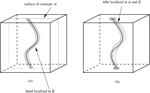
Figure 2: For simplicity, in this figure, each classical trajectory is represented by a single line, so that the box represents a gauge-fixed version of superspace with a fixed choice of lapse and shift functions defining each classical solution. The three dimensions of the box represent the $\alpha_{I}$ and $\beta_{I}$ degrees of freedom and the time direction. (a) shows a narrow band of trajectories with a fixed value of $\alpha_{I}$ and with different values of $\beta_{I}$. The choice of $S_{HJ}$ fixes the value of the $\alpha_{I}$ – the surface shown – and the prefactor then determines the region of superspace on which the functional has support – the band within the surface. The bold line indicates a mean trajectory which is surrounded by other sample trajectories. (b) more accurately represents a quasi-classical state. Since we are considering a superposition of $\alpha_{I}$ eigenstates, the wave functional has support off the surface of constant $\alpha_{I}$, and throughout a narrow tube centered around the mean trajectory. The lines represent classical trajectories with different values of both $\alpha_{I}$ and $\beta_{I}$ in the neighbourhood of the mean trajectory which is shown in bold.

5 Beyond the semiclassical approximation

The fact that a quasiclassical wavefunctional for gravity (31) has support on a tube in superspace rather than on a single eikonal track provides some elementary intuition about going beyond the simple picture of quantum field theory on a single background spacetime. As was mentioned at the end of the last section, there is no preferred choice of classical background from among all of those contained within the tube, and so if the semiclassical approximation is to hold, the physics of the matter fields had better be independent of this choice.

When one wants to talk about quantum gravity either outside or beyond the semiclassical approximation, one has a fundamental problem: The lack of a background spacetime, and of the notion of matter fields living on that background makes life difficult, since it is unclear what is meant by a unitary theory and how to define an inner product under these circumstances. Our discussion of the semiclassical approximation suggests that some or all of these concepts make sense only to the same order as the semiclassical approximation, but nonetheless form the basis of our current description of nature. The semiclassical approximation using states is in this sense much the same as the sentiments expressed over the years by Wheeler [25], since the Planck scale uncertainties in $\alpha_{I}$ and ${\beta_{I}}$ can be related to fluctuations in the underlying spacetimes which are generically on the Planck scale.

In this section we shall examine what we can learn qualitatively about corrections arising from geometry fluctuations. A careful analysis of corrections to the semiclassical approximation was carried out by Kiefer and Singh [26] by expanding the semiclassical approximation to third order. These authors derived a series of correction terms to the functional Schrödinger equation, consisting of corrections in the integration of matter fields along eikonal tracks and interference effects between eikonal tracks. In Ref. [26] the former were shown to be small, but the corrections due to interference, proportional to

$${\delta\chi[f,h_{ij}]\over\delta h_{ij}}$$ (33)

projected in a direction transverse to the eikonal trajectories, were neglected. We shall take a geometrical approach to the computation of these interference effects.

The basic quantity we wish to estimate is the state of matter on any given hypersurface $\bar{h}_{ij}$

$$\Psi_{\bar{h}_{ij}}[f]\equiv\Psi[f,\bar{h}_{ij}].$$

To the order of the semiclassical approximation (equations (18) and (19)), the evolution of this state is given by taking $\bar{h}_{ij}$ to be embedded only in the spacetimes labeled by $\bar{\alpha_{I}}$ and some ${\beta_{I}}$. Then one finds that $\Psi_{{h}_{ij}}[f]$ is a solution to the functional Schrödinger equation on a fixed background.

A set of corrections to this approximation come from taking into account the contributions from all the possible spacetimes labeled by $\alpha_{I}$ and ${\beta_{I}}$ which are not damped in the Gaussian state and which pass through $\bar{h}_{ij}$. A simple way to get qualitative information about these corrections is to consider solving the functional Schrödinger equation on all of these spacetimes and comparing the properties of the solutions. In order to solve the functional Schrödinger equation for the set of spacetimes defined by (31), it is necessary to give initial data on each of them (that is on a surface in superspace transverse to the tube). Sticking to the philosophy that we wish to construct as classical a state as possible, this initial data should be arranged to make the corrections to the semiclassical approximation as small as possible.

If there are to be only Planck scale corrections to the semiclassical approximation, the difference between Schrödinger evolution of matter states on each of the spacetimes should be small, except at the Planck scale. If this difference were large, the results obtained to the order of the semiclassical approximation would not be consistent. It is clear that one situation in which the semiclassical approximation breaks down unexpectedly is when the evolution of the matter state has sensitive dependence on the $\alpha_{I}$ and ${\beta_{I}}$ parameters.

When comparing Schrödinger evolutions on different backgrounds, we need to compare different $\Psi[f,\bar{h}_{ij}]$ for the same $\bar{h}_{ij}$. This must be done in a coordinate invariant fashion and without reference to a spacetime. Some discussion of this issue can be found in Ref. [16]. The comparison of states on entire hypersurfaces is fairly straightforward, but this does not provide a local description of the interference effect. A local comparison of matter states can be made by using matter correlation functions in the different spacetimes within the Gaussian spread. Since the basic variables are 3-metrics, an insertion point (i.e. an event) can only be defined geometrically by its position on a 3-geometry (one might for example define a hypersurface by its intrinsic geometry and then fix a point by its value of the intrinsic curvature). A correlation function should thus be defined by a 3-geometry that contains all the insertion points, and by the location within the given 3-geometry of the points. On a single classical background, the same correlation function can be defined using many different choices of a 3-geometry that passes through all the insertion points. However, quantum mechanically all of these choices are different. When we come to compute the correlation function on different spacetimes within the tube, each choice of 3-geometry identifies a different set of alternative classical spacetimes in which the 3-geometry can be embedded, and so gives different results (see Fig. 3(a)). Forcing an embedding of both surfaces into a second spacetime is possible locally, but in this case the foliation dependence occurs because the location of the insertion points in this second spacetime depends on the choice of surface (see Fig. 3(b)). It follows that the size of the corrections to the semiclassical approximation obtained by comparing correlation functions depends on how one chooses to foliate the original or mean spacetime. This dependence on foliation is inevitable if we wish to compare local quantities.

Figure 3: A pair of surfaces $\Sigma_{1}$ and $\Sigma_{2}$ in a classical spacetime $M_{0}$ are each used to define three insertion points. The computation of a matter state at the points is independent of foliation on $M_{0}$. (a) When quantum gravitational corrections are computed, each surface must be embedded in a different spacetime, since two 3-geometries determine a unique solution of Einstein’s equations. Computing a correlation function after evolution in $M_{1}$ to $\Sigma_{1}$ or in $M_{2}$ to $\Sigma_{2}$ will in general give different answers. (b) If one forcibly embeds both $\Sigma_{1}$ and $\Sigma_{2}$ in $M_{1}$ locally, without worrying about global fitting, then the points will not coincide when defined with respect to the two different surfaces.

However small the dependence on the choice of foliation, for corrections to the functional Schrödinger equation, coordinate invariance is lost. In some dramatic situations where evolution with respect to certain foliations is very sensitive to small differences in $\alpha_{I}$ and $\beta_{I}$, this can lead to very different conclusions about the size of quantum gravity effects in different foliations (or frames of reference). This might look puzzling since we started off with the Wheeler–DeWitt equation which is supposed to impose coordinate invariance. Recall, however, that the familiar notion of coordinate invariance comes from the covariance of matter evolution on a fixed background spacetime, which is valid only in the semiclassical approximation. To this order, observations are independent of a choice of foliations of the mean background spacetime. It is this notion which breaks down when one takes into account the geometry fluctuations which are higher order corrections. This is because the meaning of the Wheeler–DeWitt equation is different at this next order, since the notion of diffeomorphism invariance is now a property of the combined matter–gravity system, not just of matter on a fixed background.

Generally one might expect interference effects of the kind we have described to always be restricted to the Planck scale in any reasonable models. However, it is important to note that we cannot trust our usual intuition about quantum gravity when quantifying these effects, since they are not defined by the quantities one normally associates with a breakdown in the semiclassical approximation such as large curvature or backreaction. What makes this discussion particularly relevant is that in black hole physics, quantum gravity effects that normally occur at the Planck scale can be magnified to the classical scale by the apparently chaotic behaviour of functional Schrödinger evolution on certain hypersurfaces close to the horizon. In a variety of models, it has been shown that the evolution of matter states on foliations corresponding to outside observers close to a black hole horizon is extremely sensitive to very small fluctuations in the background geometry, so that the projection of (33) transverse to the classical solution is very large (see [16], and also [17] for a related discussion). Since large corrections are present in this case for only a very specific foliation, this indicates that a breakdown in coordinate invariance accompanies the breakdown in the semiclassical approximation. In an effective description, the results of certain sets of observations near the black hole horizon are not covariant, providing an explanation for the quantum gravitational origin of the spacetime complementarity proposed by ’t Hooft [27] and Susskind [28].

6 Conclusions

We have shown that the appropriate state to consider as quasiclassical in quantum gravity is a superposition of WKB type states which is peaked around some values of the reduced phase space variables, with close to minimal uncertainty in the reduced phase space variables. A first order WKB state on the other hand is an approximate eigenstate of half of these variables and hence not adequate. When matter is present, this is perfectly compatible with the derivation of the Schrödinger equation from the Wheeler–DeWitt constraint. This makes more precise the meaning of a semiclassical approximation in quantum gravity.

Using a superposition of WKB states, we were able to give a heuristic treatment of higher order effects due to the quantum nature of the background geometry. This allowed us to see that the semiclassical approximation can be inconsistent because of the sensitivity of matter propagation to small fluctuations in the background geometry. An example of this type of situation is given by the breakdown of a semiclassical description of matter propagating on a black hole spacetime [15, 16]. We also showed that as a consequence of quantum fluctuations, coordinate invariance is lost on the Planck scale, and in certain cases, such as near the black hole, this extends to macroscopic scales.

We have not discussed in this paper how it is that a system described by the Wheeler–DeWitt equation comes to find itself in the particular state that exhibits semiclassical behaviour. There is in principle no kinematical reason to prefer this state over any other. Perhaps the most likely answer to this question is that decoherence effectively forces any state to a configuration in which observations are equivalent to those within the Gaussian state. However, the important point is that decoherence cannot drive a state towards any configuration for which the background spacetime is more classical than the one we have described.

Appendix: A two-dimensional example

The use of Hamilton–Jacobi theory to reduce to the physical degrees of freedom was discussed rather abstractly in Sec. 3. It is instructive to illustrate this using a general 1+1 dimensional dilaton gravity model. The model we shall consider was discussed by Louis-Martinez et al [30], and we shall make extensive use of their results. Related work on open and closed spacetimes can be found in Ref. [31].

A.1. Classical theory: closed universe

Let us focus primarily on the case of a closed cosmology. Consider the action,

$$S=\int_{\cal M}d^{2}x\sqrt{-g}\left[\phi R-V(\phi)\right]$$ (34)

where $x$ is a periodic coordinate (with period $2\pi$), so that ${\cal M}=S^{1}\times R$. This model reduces to minisuperspace and string inspired models for particular choices of $V(\phi)$. For example, a constant potential $V(\phi)=-4\lambda^{2}$ gives the closed universe version [32] of the CGHS model [33].

Working with the parameterization

$$ds^{2}=e^{2\rho}\left(-N^{2}dt^{2}+(dx+N_{\perp}dt)^{2}\right)$$ (35)

for the metric $g_{\mu\nu}$, the canonical variables are $\rho(x)$ and $\phi(x)$, with conjugate momenta

$$\Pi_{\phi}={2\over N}\left(N_{\perp}\rho^{\prime}+N_{\perp}^{\prime}-\dot{\rho}\right)$$ (36)

$$\Pi_{\rho}=-{2\over N}\left(\dot{\phi}-N_{\perp}\phi^{\prime}\right)$$ (37)

while the lapse and shift functions $N$ and $N_{\perp}$ are Lagrange multipliers. As usual, the Hamiltonian is just a sum of the Hamiltonian and diffeomorphism constraints

$$H=\int dx\left[N{\cal H}+N_{\perp}{\cal H}_{\perp}\right]$$ (38)

where

$${\cal H}=2\phi^{\prime\prime}-2\phi^{\prime}\rho^{\prime}-{1\over 2}\Pi_{\rho}\Pi_{\phi}+e^{2\rho}V(\phi),$$ (39)

$${\cal H}_{\perp}=\rho^{\prime}\Pi_{\rho}+\phi^{\prime}\Pi_{\phi}-\Pi_{\rho}^{\prime}.$$ (40)

The Hamilton-Jacobi equation reads

$$g[\phi,\rho]+{\delta S\over\delta\phi}{\delta S\over\delta\rho}=0$$ (41)

where

$$g[\phi,\rho]=-4\phi^{\prime\prime}+4\phi^{\prime}\rho^{\prime}-2e^{2\rho}V(\phi).$$ (42)

This is solved by the functional

$$S[\phi,\rho;C]=2\int dx\left\{Q_{C}+\phi^{\prime}\ln\left[{2\phi^{\prime}-Q_{C}\over 2\phi^{\prime}+Q_{C}}\right]\right\}$$ (43)

where $C$ is a constant,

$$Q_{C}[\phi,\rho]=2\left[(\phi^{\prime})^{2}+\left(C+j(\phi)\right)e^{2\rho}\right]^{1\over 2}$$ (44)

and

$${dj(\phi)\over d\phi}=V(\phi).$$ (45)

(43) is also invariant under spatial diffeomorphisms.

In the Hamilton–Jacobi functional (43), we see the presence of a parameter $C$ which is the $\alpha$ parameter in this problem. To deduce $C$ as a functional of $\phi$, $\rho$ and their conjugate momenta, we must invert the relations

$${\delta S\over\delta\phi}={g[\phi,\rho]\over Q_{C}[\phi,\rho]},\qquad{\delta S\over\delta\rho}=Q_{C}[\phi,\rho].$$ (46)

These lead to the definition

$$C=e^{-2\rho}\left({1\over 4}\Pi_{\rho}^{2}-(\phi^{\prime})^{2}\right)-j(\phi)$$ (47)

Similarly we can define the quantity $\beta$, which we shall call $P$ following [30], as

$$P={\delta S\over\delta C}=-\int dx{2e^{2\rho}\Pi_{\rho}\over\Pi_{\rho}^{2}-4(\phi^{\prime})^{2}}.$$ (48)

It is easy to check that $C$ and $P$ are conjugate and that they have weakly vanishing Poisson brackets with the constraints.

From Eq. (43) for the Hamilton–Jacobi functional, we can solve the classical equations of motion, using the relations

$$\Pi_{\phi}={\delta S\over\delta\phi},\qquad\Pi_{\rho}={\delta S\over\delta\rho}$$ (49)

and Eqs. (36) and (37).

For a constant potential $V(\phi)=-4\lambda^{2}$, and taking $\sigma=1$ and $M=0$, there are homogeneous solutions

$$ds^{2}={\lambda^{2}P^{2}\over\pi^{2}}e^{-2\lambda^{2}Pt/\pi}(-dt^{2}+dx^{2})$$ (50)

and

$$\phi={C\over 4\lambda^{2}}-e^{-2\lambda^{2}Pt/\pi}$$ (51)

for all values of $C$ and $P$.

Armed with a solution of the Hamilton–Jacobi equation, it is interesting to look briefly at the quantisation of this model. We may promote ${\Pi}_{\phi}$ and $\Pi_{\rho}$ to operators

$$\hat{\Pi}_{\phi}(x)=-i\hbar{\delta\over\delta\phi(x)},\qquad\hat{\Pi}_{\phi}(x)=-i\hbar{\delta\over\delta\phi(x)}$$ (52)

With any ordering of the constraints, the first order WKB approximation is of course given by

$$\Psi[\phi,\rho]=e^{iS[\phi,\rho;C]/\hbar}$$ (53)

There is however a convenient choice of operator ordering [30]

$${\cal H} = {1\over 2}g[\phi,\rho]+{1\over 4}Q_{C_{0}}[\phi,\rho]\hat{\Pi}_{\phi}Q_{C_{0}}^{-1}[\phi,\rho]\hat{\Pi}_{\rho},$$ (54)

$${\cal H}_{\perp} = \phi^{\prime}\hat{\Pi}_{\phi}+\rho^{\prime}\hat{\Pi}_{\rho}-\hat{\Pi}_{\rho}^{\prime}$$ (55)

which depends on a parameter $C_{0}$. With this choice of ordering (53) is an exact solution of the constraint equations in the particular case where the value of $C$ in $S[\phi,\rho;C]$ is equal to $C_{0}$.

Let us now use this exact solution as a first order WKB solution and continue the WKB expansion (as we did for the relativistic particle where all the first order WKB states $e^{iPx^{\pm}/\hbar}$ were exact solutions of the Klein–Gordon equation). Writing

$$\Psi[\phi,\rho]=e^{iS[\phi,\rho;C_{0}]/\hbar+iS_{1}[\phi,\rho]}$$ (56)

the equation for $S_{1}$ is

$${\delta S_{1}[\phi,\rho]\over\delta\phi}=-{g[\phi,\rho]\over Q_{C_{0}}^{2}[\phi,\rho]}{\delta S_{1}[\phi,\rho]\over\delta\rho}$$ (57)

Note that this equation is not solved by $S[\phi,\rho;C]$ because of the minus sign. We can however find an exact solution of this equation by remembering that we expect the prefactor $-i\ln S_{1}$ to be a weight function over different values of $P$, the conjugate to $C$. Indeed, if we define the functional

$$P[\phi,\rho]\equiv-{1\over 2}\int dx{Q_{C_{0}}[\phi,\rho]\over(C+j(\phi))}$$ (58)

where we have replaced $\Pi_{\rho}$ in (48) by its classical value given by the Hamilton–Jacobi functional, then an arbitrary function of $P$ solves (57) and the WKB approximation centered around $C_{0}$ is of the form

$$\Psi[\phi,\rho]={1\over D[P[\phi,\rho]]}e^{iS[\phi,\rho;C=C_{0}]}$$ (59)

If we take $D[P[\phi,\rho]]$ to be a Gaussian, then we obtain an explicit expression for the quasiclassical state to this order. Note that for a general $D[P[\phi,\rho]]$, (59) is no longer an exact solution of the constraint equation, meaning that at least some of the $S_{i}$, $i\geq 2$ must be non-zero.

A.2. Classical theory: spacetimes with boundary

The case of an open universe has been studied by various authors [31]. It has been shown that the variable $C$ is related to the ADM mass of the spacetime, while $P$, integrated throughout a spacelike slice, is related to the time at infinity (or more precisely, to the synchronization between times at infinity). These results are in keeping with the much earlier work of Regge and Teitelboim [34] on conserved charges in canonical quantum gravity in open universes.

It is interesting to note that while $P$ is associated with a constant of the motion as described in Refs. [31], a closely related quantity provides a local geometric definition of time for different hypersurfaces within a static spacetime. Consider any 1-geometry associated with a hypersurface in a static classical solution. It can be intrinsically described by the function $\phi(s)$, where $s$ is the proper distance along the hypersurface measured from some base point $B$ at infinity, and $\phi$ is the value of the dilaton field. Let $\phi_{0}(s)$ be the function defining a constant time surface $t=t_{1}$ passing through $B=\phi_{0}(0)$. Consider now a set of hypersurfaces passing through $B$ that are defined by $\phi_{i}(s)$ which differ from $\phi_{0}(s)$ only in some finite interval $0<s<s_{0}$. For $s>s_{0}$, $\phi_{i}(s)$ also define constant time hypersurfaces but at some time $t_{i}=t_{0}+\Delta t_{i}$.

Using (47) to give $\Pi_{\rho}$ in terms of $C$ and $\phi$, we can define a quantity

$$T_{i}(S)=-\int_{0}^{S}ds{\left[\left({d\phi_{i}\over ds}\right)^{2}+C+j(\phi_{i})\right]^{1/2}\over(C+j(\phi_{i}))}$$

closely related to $P$. Here $S>s_{0}$ so that the integration extends well into the region where $\phi_{i}(s)=\phi_{0}(s)$.

Now in a static coordinate system

$$ds^{2}=e^{2\rho}(-dt^{2}+dx^{2})$$

we can compute the change in the time coordinate along any hypersurface using

$$\left({dt\over dx}\right)^{2}=1-{e^{-2\rho}\left({d\phi_{i}\over dx}\right)^{2}\over\left({d\phi_{i}\over ds}\right)^{2}}.$$

Since in the static coordinate system $\Pi_{\rho}=0$, it follows that

$$\left({dt\over dx}\right)^{2}=1+{C+j(\phi_{i})\over\left({d\phi_{i}\over ds}\right)^{2}}.$$

From this expression we deduce that

$$\Delta t_{i}=\int dx{\left[\left({d\phi_{i}\over ds}\right)^{2}+C+j(\phi_{i})\right]^{1/2}\over\left({d\phi_{i}\over ds}\right)}=\int^{S}_{0}ds{\left[\left({d\phi_{i}\over ds}\right)^{2}+C+j(\phi_{i})\right]^{1/2}\over e^{\rho}\left({d\phi_{i}\over ds}\right)}.$$

By definition $\Delta t$ is zero for $\phi_{0}$, but is non-zero for any $\phi_{i}(s)$ over the region $0<s<s_{0}$.

The connection between $\Delta t_{i}$ and $T_{i}(S)$ emerges by noting that any static solution has

$$e^{\rho}=c_{0}\left({d\phi\over ds}\right)$$

where $c_{0}$ is some constant of proportionality (this can be shown using Eqs. (39) and (47)). From this it follows that

$$\Delta t_{i}(S)={T_{i}(S)\over c_{0}}.$$

References

- [1] R.Arnowitt, S. Deser and C. Misner Phys. Rev. 117, (1960) 1595.
- [2] V. Lapchinsky and V. Rubakov, Acta Phys. Pol. B10 (1979) 1041
- [3] T. Banks, Nucl. Phys. B249 (1985) 332
- [4] J. J. Halliwell Phys. Rev. D36, (1987) 3626.
- [5] A. Anderson, Phys. Rev. D42, (1990) 585.
- [6] S. Habib and R. Laflamme, Phys. Rev. D42 (1990) 4056.
- [7] P. Bergmann, Phys. Rev. 144 (1966) 1078; A. Komar, Phys. Rev. 153 (1967) 1385; A. Komar, Observables, correspondence and quantized gravitation, in Magic Without Magic, ed. J. Klauder, San Francisco, 1972.
- [8] U. Gerlach, Phys. Rev. 177 (1969) 1929.
- [9] A. Vilenkin, Phys. Rev. D39 (1989) 1116;
- [10] D. Cangemi, R. Jackiw and B. Zwiebach, Physical states in matter coupled dilaton gravity, UCLA Report No. UCLA-95-TEP-16 (hep-th/9505161).
- [11] N.C. Tsamis and R.P. Woodard, Phys. Rev. D36 (1987) 3641-3650.
- [12] D. Cangemi and R. Jackiw, Phys. Lett. B337 (1994) 271.
- [13] C. Kiefer, The semiclassical approximation to quantum gravity, Freiburg University Report No. THEP-93/27, in Canonical Gravity – from Classical to Quantum, edited by J. Ehlers and H. Friedrich (Springer, Berlin 1994) (gr-qc/9312015).
- [14] J-P. Paz and S. Sinha, Phys. Rev. D44 (1991) 1038; S. Mathur, in Banff/CAP Workshop on Thermal Field Theories, Banff, Canada, edited by F. C. Khanna et. al. (World Scientific, Singapore, 1994).
- [15] S. D. Mathur, Black hole entropy and the semiclassical approximation, MIT report No. CTP-2304, to appear in the proceedings of the International Colloquium on Modern Quantum Field Theory II at TIFR (Bombay), January 1994 (hep-th/9404135).
- [16] E. Keski-Vakkuri, G. Lifshytz, S. Mathur and M. E. Ortiz, Phys. Rev. D51 (1995) 1764.
- [17] Y. Kiem, H. Verlinde and E. Verlinde Quantum Horizons and complementarity, CERN-TH.7469/94 (hep-th/9502074).
- [18] J. Hartle, Progress in quantum cosmology, in Proceedings, 12th Conference on General Relativity and Gravitation, Boulder, 1989, edited by N. Ashby, D. F. Bartlett and W. Wyss (CUP, Cambridge, 1990).
- [19] C. J. Isham, Canonical quantum gravity and the problem of time, presented at the 19th International Colloquium of Group Theoretical Methods in Physics, Salamanca, Spain, July 1992 (gr-qc/9210011).
- [20] A. Peres Nuovo Cimento XXVI, (1962) 53.
- [21] K. V. Kuchař, Phys. Rev. D39 (1989) 1579.
- [22] D. Giulini and C. Kiefer, Consistency of semiclassical gravity, Freiburg Report THEP-94-20 (gr-qc/9409014).
- [23] H. Goldstein Classical Mechanics, Addison-Wesley publishing Company, (1980).
- [24] C. Crnkovic and E. Witten, Covariant description of canonical formalism in geometrical theories, in Three Hundred Years of Gravitation, eds. S. Hawking and W. Israel, Cambridge University Press, Cambridge, UK 1987.
- [25] See for instance C. Misner, K. Thorne and J. A. Wheeler, Gravitation, W. H. Freeman, San Francisco (1971).
- [26] C. Kiefer and T. Singh, Phys. Rev. D44, (1991) 1067.
- [27] G. ’t Hooft, Nucl. Phys. B335 (1990) 138, and references therein.
- [28] L. Susskind, Phys. Rev. D49 (1994) 6606.
- [29] J-G. Demers, private communication.
- [30] D. Louis-Martinez, J. Gegenberg and G. Kunstatter, Phys. Lett. B321(1994) 193
- [31] T. Banks and M. O’Loughlin, Nucl. Phys. B362 (1991) 649; A. Ashtekar and J. Samuel, Bianchi cosmologies: the role of spatial topology, Syracuse Report PRINT-91-0253 (1991); K. V. Kuchař, Geometrodynamics of Schwarzschild black holes, Utah Preprint UU-REL-94/3/1, (gr-qc/9403003); H. A. Kastrup and T. Thiemann, Nucl. Phys. B425 (1994) 665.
- [32] F. D. Mazzitelli and J. G. Russo, Phys. Rev. D47 (1993) 4490.
- [33] C. G. Callan, S. B. Giddings, J. A. Harvey and A. Strominger, Phys. Rev. D 45 (1992) R1005. For reviews see J. A. Harvey and A. Strominger, Quantum aspects of black holes, in the proceedings of the 1992 TASI Summer School in Boulder, Colorado (World Scientific, 1993), and S. B. Giddings, Toy models for black hole evaporation, in the proceedings of the International Workshop of Theoretical Physics, 6th Session, June 1992, Erice, Italy, ed. V. Sanchez (World Scientific, 1993).
- [34] T. Regge and C. Teitelboim, Ann. Phys. 88 (1974) 286.