Worldsheet formulations of gauge theories and gravity

Abstract

The evolution operator for states of gauge theories in the graph representation (closely related to the loop representation) is formulated as a weighted sum over worldsheets interpolating between initial and final graphs. As examples, lattice $SU(2)$ BF and Yang-Mills theories are expressed as worldsheet theories, and (formal) worldsheet forms of several continuum $U(1)$ theories are given.

It is argued that the world sheet framework should be ideal for representing GR, at least euclidean GR, in 4 dimensions, because it is adapted to both the 4-diffeomorphism invariance of GR, and the discreteness of 3-geometry found in the loop representation quantization of the theory. However, the weighting of worldsheets in GR has not yet been found.

1 Introduction

This is a talk presented at the 7th Marcel Grossmann Meeting, held at Stanford in July ’94. It is a status report on a spacetime worldsheet formulation of quantum gauge theories (including GR) which the author has been developing Most proofs are omitted.

The idea of this reformulation of gauge theories is to express the evolution operator for states in the loop representation [GT84] [GT86] [RS88] [RS90] as a sum over 2-surfaces interpolating between initial and final loops (see Fig. 1) The overcompleteness of the loop basis complicates the situation somewhat. It is easier to work with the closely related graph basis (defined in Section 2), associated with graphs whose edges, and vertices, carry gauge group representations, instead of loops. In the worldsheet formulation described in the present paper the evolution operator in the graph representation is expressed as a sum over 2-surfaces interpolating between initial and final graphs. See Fig. 1.

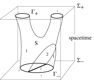
Figure 1: In the worldsheet formulation the amplitude, $U^{\Gamma_{+}}{}_{\Gamma_{-}}$, to evolve from graph state $|\Gamma_{-}\rangle$ on the initial hypersurface $\Sigma_{-}$, to graph state $|\Gamma_{+}\rangle$ on the final hypersurface $\Sigma_{+}$ is given by a sum over interpolating, possibly branched, 2-surfaces $S$. Both the edges, and vertices of valency $r>3$ of the graph and the simple components, and lines of intersection with $r>3$ of $S$ carry irreducible representations of the gauge group.

The chief motivation for developing this version of loop quantization is that it makes the 4-diffeo invariance of generally covariant theories manifest: the weight of each interpolating worldsheet $S$ depends only on the 4-diffeo equivalence class of $S$. Thus the worldsheet integral becomes a sum over 2-knots (or, more precisely, 2-tangles).

A second reason for pursuing a worldsheet formulation is that it may reveal a microstructure of spacetime mandated by GR. In canonical loop quantization it has been found [Smo91] that the quantization of the classical area observable of a 2-surface essentially counts the (unsigned) number of crossings of loops through the 2-surface. of loops (see Fig. 2).

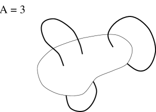
Figure 2: According to [Smo91] both the area operator of a surface $\sigma$ and the volume operator of a region of space, $\mu$, are block diagonalized in the loop basis (and, by a simple extension, in the graph basis) in the sense that they act only within the subspaces of loops, or graphs, having the same shadow, i.e., those having the same edges, differing only in the structure of their intersections. On loop states labeled by collections, $\gamma$, of smooth closed loops the area of $\sigma$ is
$A=\frac{\sqrt{3}}{2}\ (\mbox{Plank length})^{2}\times(\#\ \mbox{intersections of $\sigma$ with $\gamma$})$.
On the full state space the spectra are more complicated, but still discrete.

Thus the loop basis states can be thought of as eigenstates of the 3-geometry of space, and the 3-geometries in the spectrum are “discrete” and determined by the loops. One expects that the sum over worldsheets in the evolution operator represents a sum over discrete spacetime geometries specified by the worldsheets (in which, for instance, the area of a spacetime 2-surface is determined by the number of its intersection points with the loop worldsheet).

A final, concrete, motivation is to check the loop Hamiltonian constraint. By transforming GR from a spacetime connection form directly to a worldsheet form and then going, by a Legendre transformation, to the canonical loop formulation the Hamiltonian constraint can be derived in a new way (see Fig. 3). The derivation of the Hamiltonian constraint has, so far, been the least “natural” step in the loop quantization program.

Figure 3: Maps connecting various forms of classical and quantum GR. The bold lines mark the “beaten paths” thought to be well understood. The loop transform, represented by a bold, dashed arrow, is becoming better understood [AL93]. The author proposes to establish the top chain of links, from the classical Plebanski action to a worldsheet path integral, and then down to the canonical loop representation formulation of GR.

The features of a worldsheet formulation of GR have been described tentatively because no such formulation is known as yet. However, the author has developed, 1), a worldsheet form of $U(1)$ gauge theories in the continuum and, 2), a world sheet form of $SU(2)$ gauge theories formulated on an arbitrary, not necessarily hypercubic, lattice. Using these results, explicit worldsheet actions have been found for regulated, euclidean, compact EM, $U(1)$ F-F dual theory, a $U(1)$ analogue of GR, $SU(2)$ BF theory and $SU(2)$ lattice YM theory. Euclidean GR can be thought of as an $SU(2)$ gauge theory of the left-handed spin connection [Ple77] [CDJ91]. The corresponding worldsheet formulation is being developed by the author.

Before describing the above results in a little more detail, let’s outline how the $SU(2)$ lattice worldsheet formulation is derived.

2 Derivation of the worldsheet formulation

The most obvious basis of $SU(2)$ gauge invariant states on a lattice is the loop basis, given in the link representation by the Wilson loops $W_{\gamma}$ (see Fig. 4a).

$$\langle\{g_{l}\}_{l\in\mbox{\scriptsize links}}|\gamma\rangle=\prod_{l\in\gamma}g_{l}=W_{\gamma}$$ (1)

(A given link, $l$, may appear in the loop, $\gamma$, several times). This basis is overcomplete. There is a convenient, complete, and linearly independent basis closely related to the loop basis. It will be called the “graph” basis here. Its elements are labeled by graphs, $\Gamma$, consisting of edges labeled or “colored” by the spins $j\in\{\frac{1}{2},1,\frac{3}{2},2,...\}$ of non-unit irreducible representations of SU(2), and vertices, of arbitrary valency $r$, colored by $r-3$ $j$’s.(see Fig 4b). The function, $\Gamma(\{g_{l}\})\equiv\langle\{g_{l}\}_{l\in\mbox{links}}|\Gamma\rangle$, representing the graph basis state $|\Gamma\rangle$ in the link representation is given by a factor $U^{(j_{e})m_{+}m_{-}}(g_{e})$ for every edge $e\in\Gamma$ (with $g_{e}=\prod_{l\in e}g_{l}$ ordered along $e$) contracted on $m$’s with a factor $({}^{j_{1}}_{m_{1}}{}^{...}_{...}{}^{j_{r}}_{m_{r}})_{J_{1}...J_{r-3}}$ for each ($r$-edge) vertex. $U^{(j)}(g)$ is the spin $j$ representation of $g\in SU(2)$, and $({}^{j_{1}}_{m_{1}}{}^{...}_{...}{}^{j_{r}}_{m_{r}})_{J_{1}...J_{r-3}}$ is the generalized Wigner coefficient defined in [YLV62].

$({}^{j_{1}}_{m_{1}}{}^{...}_{...}{}^{j_{r}}_{m_{r}})_{J_{1}...J_{r-3}}$ is obtained by expanding the vertex into a tree graph with $r$ external legs and $r-2$ oriented, trivalent vertices connected by $r-3$ internal edges carrying spins $\{J_{i}\}$ and link variables $\{g_{i}={\bf 1}\}$, and contracting with $3-j$ symbols at each 3-vertex. At each vertex a conventional choice must be made of which tree graph to use in the expansion. The internal spins $\{J_{i}\}$ label distinct states within the same graph basis. Different choices of trees, on the other hand, lead to different graph bases. The expansion of vertices is illustrated in Fig. 4c.

Figure 4: Panel a) illustrates a loop state. A closed line travels along the links of the lattice, possibly returning to the same link. Each line segment along a link represents a factor $U^{(\frac{1}{2})}(g)$, the fundamental representation matrix of the link variable $g$, with one index associated with each end of the segment. The connections of the segments represent the contractions of the indices of the $U^{(\frac{1}{2})}$s.
Panel b) illustrates a graph state. A closed graph lies on the links of the lattice, with at most one line segment on each link. The line segments each represent a factor $U^{(j)}(g)$, where the (non-zero) spin $j$ is given by the color of the line. Note that the states shown in a) and b) are not equivalent, although a) is present in an expansion of b) into loop states.
Panel c) illustrates the expansion of a colored 4-valent vertex into a colored trivalent graph, which is used in the definition of graph states.

The graph basis, as well as several ideas used here, are found, at least implicitly, in Ooguri’s paper [Oog92]. Since MG7 two papers have appeared discussing the graph basis in detail: [RS94] and [Bae94].

$SU(2)$ graph states can be expanded in loop basis states by writing the spin $j$ representation matrices $U^{(j)}$ as symmetrized outer products of $2j$ factors of the corresponding fundamental representation matrix $U^{(\frac{1}{2})}$
($U^{(j)}_{m_{+}}{}^{m_{-}}=U^{(\frac{1}{2})}_{(M_{+,1}}{}^{(M_{-,1}}U^{(\frac{1}{2})}_{M_{+,2}}{}^{M_{-,2}}\ ...\ U^{(\frac{1}{2})}_{M_{+,2j})}{}^{M_{-,2j})}$, $m_{\pm}=\sum_{n=1}^{2j}M_{\pm,n}$). For example,

The graph states are orthogonal with respect to the simple, positive definite inner product

$$\langle\theta|\psi\rangle=\prod_{l\in\mbox{\scriptsize links}}\int_{SU(2)}\theta^{*}(\{g_{l}\})\ \psi(\{g_{l}\})\ dg_{l},$$ (2)

where $dg$ is the invariant, or Haar, measure on the gauge group $SU(2)$, with $\int_{SU(2)}dg=1$. The graph states are normalized by multiplying by a factor $\sqrt{2j+1}$ for each edge, including the fictitious ones in the expansion of vertices into trivalent trees. From now on, the graph states will be assumed to be normalized.

The coefficient of each graph state in the graph expansion of an arbitrary state is easily found:

$$|\psi\rangle=\sum_{\Gamma}|\Gamma\rangle\langle\Gamma|\psi\rangle.$$ (3)

Note that states in the loop representation of Gambini and Trias, and Rovelli and Smolin [GT84] [GT86] [RS88] [RS90] are functions of loops defined by $\psi[\gamma]=\langle W_{\gamma}^{*}|\psi\rangle$. $\psi[\gamma]$ is not, in general, the coefficient of $|\gamma\rangle$ in an expansion of $|\psi\rangle$ on the loop basis. In other words, $|\psi\rangle\neq\sum_{\gamma}|\gamma\rangle\langle W_{\gamma}^{*}|\psi\rangle$. The great advantage of the graph representation is that the analogous equation, (3), does hold. The quantity we want to represent as a sum over worldsheets is the evolution operator $\hat{U}$. (In diffeo invariant theories this is just the projector to the physical state space). It maps the state, $|\psi_{-}\rangle$, of the field on the initial time hypersurface, $\Sigma_{-}$, to its evolved image, $|\psi_{+}\rangle$, on the final time hypersurface, $\Sigma_{+}$.

$$|\psi_{-}\rangle=\hat{U}|\psi_{+}\rangle.$$ (4)

Expanding both $|\psi_{+}\rangle$ and $|\psi_{-}\rangle$ in graph basis states leads to

$$|\psi_{+}\rangle = \sum_{\Gamma_{+}}\sum_{\Gamma_{-}}|\Gamma_{+}\rangle\langle\Gamma_{+}|\hat{U}|\Gamma_{-}\rangle\langle\Gamma_{-}|\psi_{-}\rangle$$ (5)

$$\equiv \sum_{\Gamma_{+}}\sum_{\Gamma_{-}}|\Gamma_{+}\rangle\ U^{\Gamma_{+}}{}_{\Gamma_{-}}\ \langle\Gamma_{-}|\psi_{-}\rangle.$$ (6)

$U^{\Gamma_{+}}{}_{\Gamma_{-}}$ is the coefficient of $|\Gamma_{+}\rangle$ in the evolved image of $|\Gamma_{-}\rangle$.

In the link representation (in which states are written as functions of the set of link variables $\{g_{l}\}$) the evolution operator is given by a Feynman “path integral” over link variables belonging to links in the spacetime region ${\cal M}$, bounded by $\Sigma_{+}$ and $\Sigma_{-}$:

$$U^{\{g_{l_{+}}\}}{}_{\{g_{l_{-}}\}}=\prod_{l\in{\cal M}-\Sigma_{+}\cup\Sigma_{-}}\int_{G}dg_{l}\ e^{i\,I}$$ (7)

where the action $I(\{g_{l}\})$ depends on the $g_{l}$ of all $l\in\bar{\cal M}={\cal M}\cup\Sigma_{+}\cup\Sigma_{-}$.

Translating this into the graph representation yields

$$U^{\Gamma_{+}}{}_{\Gamma_{-}} = \langle\Gamma_{+}|\hat{U}|\Gamma_{-}\rangle$$ (8)

$$= \prod_{l\in\bar{\cal M}}\int_{G}dg_{l}\ \Gamma_{+}^{*}\ e^{i\,I}\ \Gamma_{-}.$$ (9)

Gauge invariance implies that the Feynman weight, $e^{i\,I}$, can always be written as a sum of products of factors associated with plaquettes.

$$e^{i\,I} = \sum_{\{j_{p}\}}\ \ [\ \sum_{\{m\}}c_{\{j_{p}\},\{m\}}\prod_{p\in\mbox{\scriptsize plaquettes}}f_{p}\ ]$$ (10)

$$f_{p} = U^{(j_{p})}(g_{l_{1}})\otimes U^{(j_{p})}(g_{l_{2}})\otimes...\otimes U^{(j_{p})}(g_{l_{n}}).$$ (11)

The links $l_{1},...,l_{n}$ make up the boundary of $p$. $\{m\}$ in the sum (10) refers to the indices of the matrices $U^{j_{p}}_{m_{l+}}{}^{m_{l-}}(g_{l})$ in the outer product $f_{p}$. ($m_{l-}$ is associated with the beginning of the link $l$, and $m_{l+}$ with the end).

In a given gauge theory there is a great deal of lattitude in the choice of coefficients $c$ in (10). Theories are “local” if $c$ can be chosen to be a product of factors $c_{s}$, each correlating only the link variables $g_{l}$ of links touching that site. The $c_{s}$ are to depend only on the $j$s of plaquettes touching $s$, and on indices $m$ associated with $s$.

This notion of locality seems fairly reasonable in the link formulation. It holds, in particular, for $SU(2)$ BF and YM theory. Moreover, if a gauge theory is local in this sense, in its worldsheet form the worldsheet will only interact locally.

In the terms of (10) each plaquette carries a particular irrep $j_{p}$. In fact, each term in the sum over $\{j_{p}\}$ can be visualized as a collection of patches of surface, namely the occupied plaquettes $\{p|j_{p}\neq 0\}$, labeled or “colored” by their $j_{p}\in\{\frac{1}{2},1,\frac{3}{2},2,...\}$. (See Fig. 5a.) The sum over $\{j_{p}\}$ in (10) can thus be seen as a sum over surfaces (with boundaries inside $\cal M$, in general) and the coloring of these surfaces.

Expanding the integrand in (9) according to (10) and carrying out the integral over the link variables leads to an expression for the evolution operator a sum over colored surfaces.

Let me stop to mention here a slightly different form of the expansion (10), which leads to a slightly different expression for the evolution operator. Each of the factors $U^{(j_{p})}$ in (10) can be expanded as an outer product of $2j_{p}$ factors of $U^{(\frac{1}{2})}$, symmetrized on first and second indices separately. This expanded form of the terms in (10) can be visualized by replacing each occupied plaquette in the colured surface picture by a stack of $2j_{p}$ copies of itself. (See Fig. 5b). Each edge $l$ of the colored plaquette, which represents $U^{(j_{p})}(g_{l})$, is thus replaced by $2j_{p}$ edges, each representing a factor of $U^{(\frac{1}{2})}(g_{l})$. This is the “elementary surface” picture of the terms in (10). Note that the expansion of spin $j_{p}$ edges into $2j_{p}$ spin $\frac{1}{2}$ edges, used to go from the colored surface picture to the elementary surface picture, is exactly the same as that used to expand colored graph basis states in loop basis states.

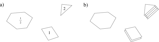
Figure 5: Panel a) shows a term in the sum (10) in the colored surface formulation. The numbers on the polygons, which represent occupied plaquettes, are the spins, $j_{p}$, they carry. Panel b) shows the elementary surface picture of the same term. Each plaquette in a) is replaced by $2j_{p}$ copies of itself.

Back to the colored surface formulation. Inserting (10) in (9) yields an expression for the evolution amplitude which is both a sum over $\{j_{p}\}$ and an integral over the link variables $\{g_{l}\}$. The integration over the $\{g_{l}\}$ of each term in the sum over $\{j_{p}\}$ is easily carried out. The integral is zero unless the surface, $\{p|j_{p}\neq 0\}$, is continous and its edges on $\partial{\cal M}$ match up with the final and initial graphs, $\Gamma_{+}$ and $\Gamma_{-}$, both in space and in coloration. The evolution amplitude can, therefore, be written as a sum over continuous (but possibly branched) surfaces interpolating between $\Gamma_{-}$ and $\Gamma_{+}$. For such continuous interpolating surfaces the integral over $\{g_{l}\}$ yields an outer product of SU(2) invariant tensors (constructed from Wigner 3-j symbols) which contract the indices of the coefficient $c$ in (10) to give the weight $e^{i\,I(S)}$ of $S$ in the sum. Thus

$$U^{\Gamma_{+}}{}_{\Gamma_{-}}=\sum_{\{S|\partial S=\Gamma_{+}\cup\Gamma_{-}\}}e^{i\,I(S)}.$$ (12)

The symbol $S$ stands for both the surface and it’s coloration.

$S$ is the union of a collection of simple (unbranched) surfaces, $\sigma$, bounded by lines on which $3$ or more simple surfaces join. Only those $S$ on which each simple component carries a single uniform color $j_{\sigma}$ contribute to (12). (see Fig. 6a). Furthermore the colors of simple components joining at a line must satisfy polygon inequalities, i.e., the $j$’s must be the edge lengths of a closed polygon of integral perimeter. See Fig. 6b for an illustration of an illuminating alternative formulation of this requirement.

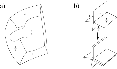
Figure 6: Panel a) illustrates that $S$ in (12) is the union of monochrome simple surfaces bounded by lines on which $3$ or more surfaces meet. The simple components can have nontrivial topology and need not be orientable in SU(2) theories. There can also be transverse intersections of simple components at points. Note that at most one simple component traverses a given plaquette. Panel b) illustrates the polygon inequalities at lines of intersection. One way of stating these is that there must exist a routing of simple surfaces through the line of intersection so that $2j_{\sigma}$ such surfaces enter (or exit) the line of intersection along each simple component $\sigma$ of $S$ meeting at the line, with none of the surfaces returning along the same component.

Instead of colored surfaces one may work with elementary surfaces. Proceeding in exact analogy to the derivation of the colored surface formulation one finds an expression for the evolution amplitude from the initial to the final graph basis state as a sum over continous, elementary surfaces which interpolate between loops present in the decomposition of $|\Gamma_{+}\rangle$ and $|\Gamma_{-}\rangle$ into loop basis states. Unlike the colored surfaces the elemetary surfaces can traverse a given plaquette several times. The elementary surfaces are not branched, in the sense that there are no lines on which $3$ or more non-coplanar surfaces join. However, there can be branch cuts ending at branch points, as occur on Riemann surfaces.

This completes the outline of the derivation of the world sheet formulation of general $SU(2)$ gauge theories. For $U(1)$ theories the world sheet formulation can be derived analogously, on a lattice, or directly in the continuum by a method which will not be discussed here.

3 Worldsheet forms of some specific theories

Let’s first summarize the results for $U(1)$ theories. In the conection formulation, which we take as our starting point, these are theories of $U(1)$ fiber bundle geometries, described by a curvature, or field strength, 2-form $F$. In a neighborhood about any point not on a magnetic monopole worldline one can find a 1-form potential $A$ such that $F=d\wedge A$. The $U(1)$ bundle is not assumed trivial, so Dirac monopoles are allowed, at least kinematically.

In the worldsheet formulation of $U(1)$ theories the evolution operator is a sum, weighted by the world sheet Feynman weight $e^{i\,I_{s}}$, over oriented 2-surfaces interpolating between initial and final graphs.

Oriented 2-surfaces can be added and multiplied by integers in the sense that $\int_{mS_{1}+nS_{2}}=m\int_{S_{1}}+n\int_{S_{2}}$, so they form an infinite dimensional lattice, even in the continuum. The sum over surfaces in the elementary surface formula for the evolution operators of $U(1)$ theories are sums over this lattice, with equal a priori weights for each lattice point. Whether the sums are well defined depends on the Feynman weight function of the particular theory being considered.

For regulated Euclidean compact electrodynamics with connection action $I_{c}[A]=\frac{1}{4}\int F_{\mu\nu}F_{\lambda\rho}\eta^{\mu\lambda}\eta^{\nu\rho}d^{4}x$ the surface action is

$$I_{s}(S)=\frac{e^{2}}{\Lambda^{2}}\int_{S}n^{2}d(\,area\,)$$ (13)

where $\Lambda$ is the regulator length, $e$ is the fundamental electric charge, and $n(x)$ is the representation of $U(1)$ at $x$ on the surface $S$. In the elementary surface formulation the action is still (13), with $n(x)$ the is the number of layers of elementary surface at $x$. It is interesting that, besides the $n^{2}$ dependence, this is just the Nambu-Goto action of string theory. The summation over worldsheets appears to be well defined in this theory.

Compact EM has a well known [BMK77] phase transition from a strong coupling phase, in which electric charges are confined, to a weak coupling phase, in which charges are unconfined and the EM field consists of a collection of non-interacting photons. This transition is currently being studied in the worldsheet formalism. Preliminary indications are that the worldsheet action (13) describes this transition. At the transition the elementary surface form of the worldsheet sum is dominated by spacetime filling worldsheets. Thus the $n^{2}$ factor in the the lagrangian of (13) becomes important at the transition.

F - F dual theory, with $I_{c}[A]=k\int\epsilon^{\mu\nu\lambda\rho}F_{\mu\nu}F_{\lambda\rho}\ d^{4}x=k\int F\wedge F$ has the surface action

$$I_{s}(S)=-\frac{e^{2}}{4k}\ \sum_{i={\rm intersection\ of}\ S}sgn(i)\ n_{1}n_{2}$$ (14)

where $n_{1}$ and $n_{2}$ are the $U(1)$ representations carried by the intersecting pieces of $S$, and $sgn(i)$ is the sign of the intersection. See Fig. Note that $n\rightarrow-n$ if the orientation of $S$ is reversed.

The F - F dual theory is a (somewhat trivial) diffeo invariant theory. Our expectation that world sheet actions of diffeo invariant theories depend on the diffeo equivalence class of the world sheet only is confirmed in the case of this theory. It is not so easy check, however, that the sum over worldsheets is diffeo invariant.

The third $U(1)$ theory the author has examined might be called $U(1)$ gravity. It is diffeo invariant, but it is not a topological theory, having an infinite dimensional state space. Its action is the closest $U(1)$ analogue of the Plebanski action for GR. The Plebanski action for GR is [Ple77][CDJ91][Pel93]:

$$I[\Sigma,A]=\int\Sigma_{a}\wedge F^{a}+\phi^{ab}\Sigma_{a}\wedge\Sigma_{b}$$ (15)

where $A$ is the left-handed spin connection (which takes its values in complexified $su(2)$), $F$ is its curvature, and $\Sigma$ is an $su(2)$ valued 2-form. $\phi^{ab}$ is a symmetric, trace free, matrix in the $su(2)$ indices, which acts as a lagrange multiplier. The $U(1)$ gravity action is obtained from (15) by dropping the $su(2)$ indices:

$$I[\Sigma,A]=\int\Sigma\wedge F+\phi\Sigma\wedge\Sigma.$$ (16)

The worldsheet form of this theory is a little different from that of the preceding theories. Integrating out the lagrange multiplier produces a delta function in the sum over surfaces (12) that restricts this sum to surfaces satifying a condition at intersections. Namely, at an intersection of $r$ parts of $S$

$$\sum_{a,b}sgn(i_{a,b})n_{a}n_{b}=0$$ (17)

where $a,b\in\{1,...,r\}$ label the intersecting parts of $S$. On allowed surfaces the action is identically zero. Thus the evolution operator is given by a democratic sum over a restricted class of allowed surfaces. Note that, as expected, the restriction is diffeo invariant. Possibly the evolution operator for GR is given by a similar sum over a restricted class of surfaces.

Besides $U(1)$ theories the author has also worked out the worldsheet formulation of lattice $SU(2)$ BF theory and YM theory.

The connection action for BF theory is

$$I_{c}=\int tr[B\wedge F]$$ (18)

where $B$ is an $su(2)$ valued 2-form, like $\Sigma$ in the Plebanski action (15). (18) is just the Plebanski action without the lagrange multiplier term.

In the lattice, link formulation BF theory has the Feynman weight

$$e^{i\,I}=\sum_{\{j_{p}\}}\prod_{p\in{\rm plaquettes}}tr[\prod^{\rightarrow}_{l\in\partial p}U^{(j_{p})}(g_{l})]$$ (19)

$\prod^{\rightarrow}_{l\in\partial p}$ is the path ordered product around $\partial p$, so $tr[\prod^{\rightarrow}_{l\in\partial p}U^{(j_{p})}(g_{l})]=W_{\partial p}^{(j_{p})}$. The Wilson loop $W_{\partial p}^{(j_{p})}$ can also be written as a trace of $f_{p}$, so (19) is of the form (10).

The Feynman weight of a worldsheet, $S$, in the colored surface formulation of this theory is obtained by applying the machinery of the last section to (19). It is given by a factor $(2j+1)^{\chi}$ for each simple component of $S$, $\chi$ being the Euler charactersitic of the component, and a Racah-Wigner symbol for each point of intersection (where several lines of intersection meet).

$$e^{i\,I(S)}=\prod_{\sigma\in\mbox{\scriptsize simple components}}(2j_{\sigma}+1)^{\chi_{\sigma}}\prod_{\mbox{\scriptsize intersection points}}\mbox{R-W symbol}$$ (20)

The Racah-Wigner symbol associated with an intersection is computed by placing a small 3-sphere around the intersection point, so that each surface meeting at the intersection point cuts the sphere along a line (including, of course, the 2-cells of the tree surface used to expand lines of intersection of valency $r>3$). These lines form a trivalent graph labeled by the $j$’s of the surfaces (of the same form as the graphs labeling the graph basis, when their vertices are expanded into trivalent trees). The Racah-Wigner symbol associated with the intersection is the evaluation, according to the rules of [YLV62], of this graph. That is, it is the value of the link rep. graph wavefuction evaluated on a flat connection on the sphere. Fig 7 illustrates this the evaluation of intersection factors.

Figure 7: The evaluation of the intersection factor associated with the meeting of four trivalent lines of intersection in $2+1$ GR (= $2+1$ BF theory) is shown. A sphere is placed around the intersection point, and the graph on which the intersecting surfaces cut the sphere is extracted. This is just a tetrahedron with the spins of the surfaces labelling the corresponding edges. This tetrahedron is then evaluated as a 6-j symbol.

The resulting theory is easily shown to be equivalent to Ooguri’s [Oog92] simplicial formulation of BF theory. $2+1$ dimensional GR leads to exactly the same worldsheet action, and the worldsheet formulation is easily seen to be equivalent to the Ponzano-Regge [PR68] form of GR. In fact, Turaev and Viro [TV92], and Kauffman and Lins [KL94] have given a formulation of $2+1$ GR virtually identical to the colored worldsheet form, but with the more general structure $SU(2)_{q}$ replacing $SU(2)$.

Note that, in BF theory, surfaces that intersect transversely (i.e. at a point) do not interact. Our experience with “$U(1)$ gravity” suggests that this is due to the absence of a $B\wedge B$ term in the action, and that in GR such surfaces will interact.

The lack of interaction of surfaces at transverse intersection points in BF theory leads the author to suspect that, in the elementary surface formulation of BF theory, surfaces do not interact at all, the complicated intersection factors in the colored surface formulation coming from counting distinct routings of elementary surfaces. Iwasaki [Iwa94] has formulated an elementary surface form of $2+1$ GR, but his result is too implicit to allow an easy check of this conjecture.

Euclidean $SU(2)$ YM theory can be defined in the continuum connection formulation by the Feynman weight

$$e^{i\,I}=\int{\cal D}B\ \ e^{i\int tr[B\wedge F]}\ e^{-g^{2}\int tr[B_{\alpha\beta}B_{\gamma\delta}]g^{\alpha\gamma}g^{\beta\delta}\sqrt{g}\epsilon},$$ (21)

like that of BF theory, except for the second factor in the integrand. $g^{2}$ is the YM coupling strength.

A very nice form of YM theory on a hypercubic lattice is provided by the heat kernel action [MO81]

$$e^{i\,I}=\sum_{\{j_{p}\}}\prod_{p\in{\rm plaquettes}}tr[\prod^{\rightarrow}_{l\in\partial p}U^{(j_{p})}(g_{l})]\ e^{-g^{2}\,j_{p}(j_{p}+1)},$$ (22)

again, just like BF theory with an extra factor in the summand. (22) then leads to a colored worldsheet Feynman weight like that of BF theory, except that each simple component contributes an extra factor $e^{-j(j+1)(\mbox{area})/a^{2}}$ ($a$ = lattice spacing), in close analogy with euclidean compact EM. This worldsheet formulation of lattice YM theory is, in fact, just a systematization of the strong coupling expansion of Wilson [Wil74], applied to the heat kernel action. See [ID89].

An elemetary surface formulation of $SU(2)$ YM theory would constitute a generalization to a 4-dimensional, lattice of the string representations of 2-d YM theory of Gross and Taylor [GT93b] [GT93a].

References

- [AL93] A. Ashtekar and J. Lewandowski. Representation theory of analytic holonomy algebras. gr-qc 9311010, 1993.
- [Bae94] J. Baez. Spin network states in gauge theory. gr-qc 9411007, 1994.
- [BMK77] T. Banks, R. Meyerson, and J. Kogut. Phase transitions in abelian lattice gauge theories. Nucl. Phys. B, 129:493, 1977.
- [CDJ91] R. Capovilla, J. Dell, and T. Jacobson. A pure spin connection formulation of gravity. Class. Quantum Grav., 8:59, 1991.
- [GT84] R. Gambini and A. Trias. On confinement in pure yang-mills theories. Phys. Lett. B, 141:403, 1984.
- [GT86] R. Gambini and A. Trias. Gauge dynamics in the C-representation. Nucl. Phys. B, 278:486, 1986.
- [GT93a] D. Gross and W. Taylor. Twists and Wilson loops in the string theory of two-dimensional QCD. Nucl. Phys. B, 403:395, 1993.
- [GT93b] D. Gross and W. Taylor. Two dimensional QCD is a string theory. Nucl. Phys. B, 400:181, 1993.
- [HK90] V. Husain and K. Kuchar. General covariance, new variables, and dynamics without dynamics. Phys. Rev. D, 42:4070, 1990.
- [ID89] C. Itzykson and J.-M. Drouffe. Statistical Field Theory. Cambridge University Press, Cambridge, 1989.
- [Iwa94] J. Iwasaki. A reformulation of the Ponzano-Regge quantum gravity model in terms of surfaces. gr-qc, 9410010, 1994.
- [Kau91] L. Kauffman. Knots and Physics. World Scientific, Singapore, 1991.
- [KL94] L. Kauffman and S. Lins. Temperley-Lieb Recoupling Theory and Invariants of 3-Manifolds. Annals of Mathematics studies. Princeton University Press, Princeton, New Jersey, 1994.
- [MO81] P. Menotti and E. Onofri. The action of SU(N) lattice gauge theory in terms of the heat kernel on the group manifold. Nucl. Phys. B, 190:288, 1981. Earlier references that make use of a heat kernel action are listed in this paper.
- [Oog92] H. Ooguri. Topological lattice models in four dimensions. Mod. Phys. Lett. A, 7:2799, 1992.
- [Pel93] P. Peldan. Actions for gravity, with generalizations: A review. gr-qc, 9305011, 1993.
- [Pen69] R. Penrose. Angular momentum: an approach to combinatorial space-time. In T. A. Bastin, editor, Quantum theory and Beyond. Cambridge University Press, 1969.
- [Ple77] J. F. Plebanski. On the separation of Einsteinian substructures. J. Math. Phys., 18:2511, 1977.
- [PR68] G. Ponzano and T. Regge. Semiclassical limit of Racah coefficients. In F. Bloch, S. Cohen, A. De-Shalit, S. Sambursky, and I. Talmi, editors, Spectroscopic and Group Theoretical Methods in Physics, page 1, Amsterdam, 1968. North Holland.
- [RS88] C. Rovelli and L. Smolin. Knots and quantum gravity. Phys. Rev. Lett., 61:1155, 1988.
- [RS90] C. Rovelli and L. Smolin. Loop representation for quantum general relativity. Nucl. Phys. B, 133:80, 1990.
- [RS94] C. Rovelli and L. Smolin. Discreteness of area and volume in quantum gravity. gr-qc, 9411005, 1994.
- [Smo91] L. Smolin. Recent developments in non-perturbative quantum gravity. In Proceedings of the 1991 GIFT seminar on Theoretical Physics: “Quantum Gravity and Cosmology”, Singapore, 1991. World Scientific.
- [TV92] V. Turaev and O. Viro. State sum invariants of 3-manifolds and quantum 6-j symbols. Topology, 31:865, 1992.
- [Wil74] K. Wilson. Confinment of quarks. Phys. Rev. D, 10:2445, 1974.
- [YLV62] A. P. Yutsis, I. B. Levinson, and V. V. Vanagas. Mathematical Apparatus of the Theory of Angular Momentum. Israel Program for Scientific Translations, Jerusalem, 1962.