CERN-TH.7516/94

On the Space-Time Geometry
of Quantum Systems

Dirk Graudenz 
Theoretical Physics Division, CERN
CH–1211 Geneva 23

We describe the time evolution of quantum systems in a classical background space-time by means of a covariant derivative in an infinite dimensional vector bundle. The corresponding parallel transport operator along a timelike curve ${{C}}$ is interpreted as the time evolution operator of an observer moving along ${{C}}$. The holonomy group of the connection, which can be viewed as a group of local symmetry transformations, and the set of observables have to satisfy certain consistency conditions. Two examples related to local $\mbox{SO}(3)$ and $\mbox{U}(1)$-symmetries, respectively, are discussed in detail. The theory developed in this paper may also be useful to analyze situations where the underlying space-time manifold has closed timelike curves.

CERN-TH.7516/94

November 1994

1 Introduction

The state vector in quantum theory is an object that describes the knowledge about a physical system. In the case of a local quantum field theory in a possibly curved space-time background, the maximum knowledge about the system can be encoded in a state vector $\Psi_{S}$ that is defined for a spacelike hypersurface $S$ [1]. This is the case because observables whose space-time supports are separated by a spacelike distance commute and can thus be separately diagonalized. In the definition of states $\Psi_{S}$ it is implicitly assumed that the space-time manifold $M$ can be foliated by a set of spacelike hypersurfaces $S_{\lambda}$, where $\lambda$ is a real parameter; see Fig. 1. The evolution of the system is then given by a Schrödinger equation of the form

$$\frac{{\mbox{d}}}{{\mbox{d}}\lambda}\,\Psi_{S_{\lambda}}\,=\,H_{\lambda}\,\Psi_{S_{\lambda}}.$$ (1)

$\lambda$ plays the rôle of a global time coordinate. The approach of slicing space-time by spacelike hypersurfaces has the disadvantage that the time evolution is not easily generalized to space-time manifolds with closed timelike curves or similar causal obstructions, since sometimes it is not possible to find a global foliation $S_{\lambda}$.

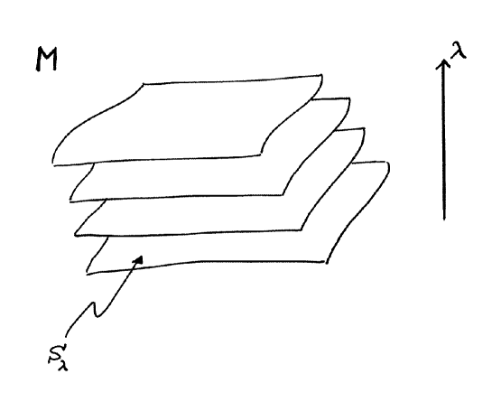
Figure 1: Foliation of space-time by spacelike hypersurfaces.

Here we try to give a formulation of quantum theory that in principle allows a description of the time evolution of a system even in the problematic cases just mentioned. The key observation is that knowledge is always knowledge by an observer $B$. Let ${{C}}_{\tau}$ be $B$’s worldline, where $\tau$ parametrizes ${{C}}$; one can think of $\tau$ as $B$’s eigentime. We will associate with every curve ${{C}}$ a state vector $\Psi_{{C}}(\tau)$ depending on the curve ${{C}}$ and on the curve parameter $\tau$. For $B$, the state evolution will be described by a Hamiltonian operator $H_{{C}}(\tau)$ in the form of a Schrödinger equation

$$\frac{{\mbox{d}}}{{\mbox{d}}\tau}\,\Psi_{{C}}(\tau)\,=\,H_{{C}}(\tau)\,\Psi_{{C}}(\tau).$$ (2)

The Hamiltonian operator depends on the space-time curve ${{C}}$. By integrating Eq. (2) we may define a unitary evolution operator $U_{{C}}(\tau,\tau_{0})$ satisfying the equation

$$\partial_{\tau}\,U_{{C}}(\tau,\tau_{0})\,=\,H_{{C}}(\tau)\,U_{{C}}(\tau,\tau_{0})$$ (3)

with the initial condition $U_{{C}}(\tau_{0},\tau_{0})={1\!\!\!\!\,\,1}$. For a curve ${{D}}:[a,b]\rightarrow M$ we may define $U_{{D}}$ by $U_{{D}}(b,a)$ (i.e. by the evolution operator from the beginning to the end of the curve). We will assume, for simplicity, that all observables under consideration are scalar quantities such that two observers $B_{1}$, $B_{2}$ at the same space-time point $x$ could use the same state vector $\Psi$ regardless of the relative orientation of their coordinate systems and their relative velocity.

For two curves ${{D}}$, ${{E}}$ with the property that the endpoint of ${{D}}$ is the starting point of ${{E}}$, let ${{E}}\circ{{D}}$ be the concatenation of ${{D}}$ and ${{E}}$, i.e. the curve that is obtained by first following ${{D}}$ and then ${{E}}$; see Fig. 2.

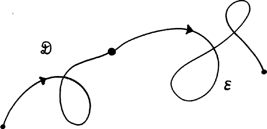
Figure 2: Concatenation of two curves.

We assume that the specific parametrisations of the curves are irrelevant; physics should be independent of the coordinates chosen. We certainly require that the evolution operators satisfy

$$U_{{{E}}\circ{{D}}}\,=\,U_{{E}}\,\circ\,U_{{D}},$$ (4)

which is a compatibility condition with Eq. (3). Moreover, we require that

$$U_{{{D}}^{-1}}\,=\,U_{{D}}^{-1},$$ (5)

where ${{D}}^{-1}$ is the curve ${{D}}$ traversed in the opposite direction. All these properties are precisely those of parallel transport operators. This fact suggests a formulation in the language of differential geometry, which will be developed in Section 1.

The connection of the vector bundle introduced there will, in general, possess a non-trivial holonomy group. Since the expectation values, predicted by two observers $B,\,C$ for a measurement at a system should not differ, the non-trivial holonomy leads to certain consistency conditions. It turns out that the consistency conditions can be interpreted as a structure of local symmetry transformations. The group of these symmetry transformations at a space-time point $x$ is a representation of the loop group at $x$. We investigate this structure in Section 1. Two examples related to local $\mbox{SO}(3)$ and $\mbox{U}(1)$-symmetries, respectively, are discussed in Section 1. The paper closes with a summary and some conclusions.

2 A Formulation in the Language of Differential Geometry

We formulate in this section the evolution of quantum systems in a differential geometric framework. As we have seen in the preceding section, the evolution operators $U_{{D}}$ have the properties of parallel transport operators. In general, they act on a fibre bundle $\pi_{G}:G\rightarrow M$ over the (connected) space-time manifold $M$. The fibre $G_{x}:=\pi_{G}^{-1}(x)$ over $x$ is isomorphic to a Hilbert space ${{H}}$. The state of the quantum system, as described by an observer at $x\in M$, is an element of $G_{x}$.

For a curve ${{D}}:[a,b]\rightarrow M$, $U_{{D}}$ maps $G_{{{D}}_{a}}$ onto $G_{{{D}}_{b}}$. Under suitable differentiablity conditions the parallel transport operators $U_{{D}}$ have an infinitesimal representation in terms of a connection or covariant derivative $D$ on the bundle $\pi_{G}$. In a local coordinate system $\Phi$ given by

$$G\Big{|}_{W}\,\stackrel{{\scriptstyle\Phi}}{{\rightarrow}}\,W\,\times{{H}},\quad W\subset M,\quad G\Big{|}_{W}\,{\stackrel{{\scriptstyle def}}{{\displaystyle=}}}\,\bigcup\limits_{x\in W}\,G_{x},$$ (6)

$D$ can be expressed as $D={\mbox{d}}-H$, where ${\mbox{d}}=\partial_{\mu}\cdot{\mbox{d}}x^{\mu}$ is the differential on $W$, and $H=H_{\mu}\,{\mbox{d}}x^{\mu}$ is an operator-valued one-form on $M$. As will be seen shortly, $H$ transforms like a gauge field under a change of the frame. In the local frame $\Phi$, the evolution operator $H_{{C}}(\tau)$ introduced above is $H_{{C}}(\tau)\,=\,H_{\mu}({{C}}_{\tau})\,\dot{{{C}}}^{\mu}_{\tau}$, where the dot denotes differentiation with respect to the curve parameter. Therefore,

$$\partial_{\tau}\,U_{{C}}(\tau,\tau_{0})\,=\,H_{\mu}({{C}}_{\tau})\,\dot{{{C}}}^{\mu}_{\tau}\,U_{{C}}(\tau,\tau_{0}).$$ (7)

Under a change of coordinates

$$\chi=\Phi_{2}\circ\Phi_{1}^{-1},$$ (8)

the representative $(x,\Psi)=\Phi_{1}(\psi)$ of a vector $\psi$ over $x$ in the frame $\Phi_{1}$ is mapped via $\chi$ into the representative $(x,V(x)\Psi)=\Phi_{2}(\psi)$ in the frame $\Phi_{2}$ , where $V(x)$ is a unitary operator on ${{H}}$ (we assume that the structure group of $\pi_{G}$ is a group of unitary operators). If $H_{\Phi_{1}}$ is the generator of parallel translations in the frame $\Phi_{1}$, then the corresponding generator $H_{\Phi_{2}}$ in the frame $\Phi_{2}$ is

$$H_{\Phi_{2}}(x)\,=\,V(x)\,H_{\Phi_{1}}(x)\,V(x)^{-1}\,+\,{\mbox{d}}V(x)\,V(x)^{-1},$$ (9)

satisfying $({\mbox{d}}-H_{\Phi_{2}})(V\Psi)=V({\mbox{d}}-H_{\Phi_{1}})\Psi$. This transformation law is that of a gauge field. The inhomogeneous term arises because the unitary transformation operator $V$ will, in general, depend on the space-time point $x$.

Up to now, we have just considered the evolution of the state vectors. We now discuss the question of observables. Let ${{M}}$ be a set of observables. We think of $A\in{{M}}$ as some scalar observable like the field strength of a scalar field. In general, however, $A$ may be any scalar quantity that can be measured by means of a suitable ‘infinitesimal measuring device’ at any space-time point. It should be noted that the observables $A$ do not carry a space-time index. In order to associate observables to space-time points, we assume that there is a mapping $\varphi$ of the set of observables into the algebra of operators on $G$, such that $\varphi(A)\equiv A_{\varphi}$ for $A\in{{M}}$ maps every fibre $G_{x}$ into itself.

In order to calculate expectation values of observables, a Hermitian inner product $P(\psi,\xi)\equiv\langle\psi|\xi\rangle$ for vectors $\psi,\,\xi$ from the same fibre of $G$ is needed. The quantity $\langle\psi|A_{\varphi}|\psi\rangle/\langle\psi|\psi\rangle$ is interpreted as the expectation value for the observable $A$ at the space-time point $x$ if the state of the system is described by an observer $B$ at $x$ by means of the state $\psi\in G_{x}$.

Let the prototype Hilbert space ${{H}}$ be equipped with the Hermitian inner product $[\cdot|\cdot]$. Then the expression $\langle\psi|A_{\varphi}|\xi\rangle$ for $\psi,\,\xi\in G_{x}$ can be written in a local frame $\Phi$ as

$$\langle\psi|A_{\varphi}|\xi\rangle=[\Phi(\psi)|P_{\Phi}(x)A_{\varphi\Phi}(x)|\Phi(\xi)],$$ (10)

where $P_{\Phi}(x)$ is a Hermitian operator (Hermitian with respect to $[\cdot|\cdot]$) representing the inner product $P$ in the fibre $G_{x}$ over $x$, and $A_{\varphi\Phi}(x)$ is a Hermitian operator (Hermitian with respect to $[\cdot|P_{\Phi}(x)\cdot]$) corresponding to the observable $A$. Under the change of frame in Eq. (8) the inner product $P$ and the operators $A_{\varphi}$ transform like

$$P_{\Phi_{2}}(x) = V(x)P_{\Phi_{1}}(x)V(x)^{-1},$$ (11)

$$A_{\Phi_{2}}(x) = V(x)A_{\Phi_{1}}(x)V(x)^{-1}.$$ (12)

We assume that the inner product $P$ and the covariant derivative are compatible. In terms of the parallel transport operators this means that

$$\langle U_{{D}}\psi|U_{{D}}\xi\rangle=\langle\psi|\xi\rangle,$$ (13)

where $\psi,\,\xi$ are vectors from the fibre of $G$ over the starting point of ${{D}}$.

So far we have considered the prediction by an observer $B$ at $x$ of expectation values for measurements of observables at $x$. We now give a prescription for the prediction of expectation values of measurements at $y\neq x$. The idea is simple: let $\psi_{B}$ be the state vector used by $B$ at $x$. Choose a curve ${{D}}:[a,b]\rightarrow M$ connecting $x={{D}}_{a}$ and $y={{D}}_{b}$ and transport $\psi_{B}$ from $x$ to $y$ via $\psi_{B}^{{D}}=U_{{D}}\psi_{B}$ along ${{D}}$. Define the expectation value for a measurement of $A$ at $y$ to be $\langle\psi_{B}^{{D}}|A_{\varphi}(y)|\psi_{B}^{{D}}\rangle$ (we assume $\langle\psi_{B}^{{D}}|\psi_{B}^{{D}}\rangle=1$). In general, $\psi_{B}^{{D}}$ depends on the curve ${{D}}$ chosen. The consistency conditions resulting from this dependence will be discussed in the next section. As a preparation of this discussion, we consider the curvature $F=D^{2}$ of the connection $D$. $F$ is an operator-valued two-form, mapping two tangent vectors $v,\,w$ of the tangent space $T_{x}M$ of $M$ at $x$ and a vector $\psi\in G_{x}$ into a vector $F(v,w)\psi\in G_{x}$. $F$ is a measure for how much the parallel transport around an infinitesimal closed loop fails to be the identity,

$$U_{\beta}={1\!\!\!\!\,\,1}+\tau^{2}F(v,w),$$ (14)

where $\beta$ is the infinitesimal closed loop ($\tau\ll 1$) connecting the points $(x,x+\tau v,x+\tau v+\tau w,x+\tau w,x)$.

3 Consistency Conditions and the Local Symmetry Structure

We now consider the dependence on the curve ${{D}}$ joining $x$ and $y$ of predictions for measurements at $y$ by an observer $B$ at $x$. Let ${{E}}$ be another curve joining $x$ and $y$; see Fig. 3. The prediction will then be $\langle\psi_{B}^{{E}}|A_{\varphi}(y)|\psi_{B}^{{E}}\rangle$. Certainly the expectation value should not depend on the path chosen, so we require

$$\langle\psi_{B}^{{D}}|A_{\varphi}(y)|\psi_{B}^{{D}}\rangle=\langle\psi_{B}^{{E}}|A_{\varphi}(y)|\psi_{B}^{{E}}\rangle.$$ (15)

Thus,

$$\langle U_{{D}}\psi_{B}|A_{\varphi}(y)|U_{{D}}\psi_{B}\rangle=\langle U_{{E}}\psi_{B}|A_{\varphi}(y)|U_{{E}}\psi_{B}\rangle.$$ (16)

This condition can be rewritten as

$$\langle U_{{D}}\psi_{B}|U_{\alpha}A_{\varphi}(y)U_{\alpha}^{-1}-A_{\varphi}(y)|U_{{D}}\psi_{B}\rangle=0.$$ (17)

Here the closed loop $\alpha$ is defined by $\alpha={{D}}\circ{{E}}^{-1}$. The condition has to be satisfied for all $y$, for all $\psi_{B}\in G_{x}$ and for all curves ${{D}},\,{{E}}$ joining $x$ and $y$. Therefore, since $U_{{D}}$ is an isomorphism, the condition

$$\langle\xi|U_{\alpha}A_{\varphi}(y)U_{\alpha}^{-1}-A_{\varphi}(y)|\xi\rangle=0$$ (18)

has to hold for all $\xi\in G_{y}$ and for all closed loops $\alpha$ located at $y$. As a consequence,

$$[U_{\alpha},A_{\varphi}(y)]=0$$ (19)

if all vectors $\xi$ are physical.

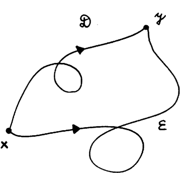
Figure 3: Path independence of expectation values.

The set of all parallel transport operators $U_{\alpha}$ along closed loops $\alpha$ located at the same point $y$ forms a group, the so-called holonomy group ${{H}}(y)$ of the connection $D$ at $y$. The relation Eq. (19) expresses the fact that the holonomy group at $y$ has to commute with all observables at $y$. The $U_{\alpha}$ transform states into states and have to leave observables invariant. This is to say that they act as local symmetry transformations. These transformations are not related to the transformations of the change of coordinates Eq. (8) in Section 1. On the contrary, they do transform state vectors non-trivially.

The holonomy group ${{H}}(y)$ is a representation of the loop group ${{L}}(y)$ of $M$ at $y$ [2]. The loop group as a set consists of classes $[\alpha]$ of closed loops at $y$, where two loops $\alpha,\,\beta$ are equivalent, $\alpha\sim\beta$, if $\beta$ can be obtained from $\alpha$ by inserting or deleting curve segments of the form ${{F}}\circ{{F}}^{-1}$, see Fig. 4. Group multiplication is defined by $[\alpha]\circ[\beta]=[\alpha\circ\beta]$, and the inverse by $[\alpha]^{-1}=[\alpha^{-1}]$. Let ${{L}}^{0}(y)$ be the subgroup of ${{L}}(y)$ consisting of the classes $[\alpha]$ of closed loops $\alpha$ which are homotopic to $0$, i.e. which can be smoothly contracted to the constant curve at $y$. Let ${{H}}^{0}(y)$ be the restricted holonomy group consisting of operators $U_{\alpha}$ for $[\alpha]\in{{L}}^{0}(y)$ (see [3]). It is known that ${{H}}^{0}(y)$ is a normal subgroup of ${{H}}(y)$, and that the factor group ${{H}}(y)/{{H}}^{0}(y)$ is discrete. The first homotopy group $\pi_{1}(M,y)$ of the space-time manifold $M$ has a representation in this discrete group. Thus the topology of space-time is partly reflected in the structure of the observable algebra in the form of a discrete factor group of the group of symmetry transformations. The condition $[U_{\alpha},A_{\varphi}(y)]=0$ for $\{\alpha\}\in\pi_{1}(M,y)$ ($\{\alpha\}$ being the homotopy class of $\alpha$) can alternatively be interpreted as a discrete ‘quantization condition’.

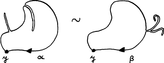
Figure 4: Equivalent closed loops.

If the set of observables ${{M}}$ is complete in the sense that the condition $\mbox{tr}(A_{\varphi}^{{D}}\rho)=0$ for a density matrix $\rho$, for all curves ${{D}}$ and for all observables $A\in{{M}}$ has the consequence that $\rho=0$, then for all closed loops $\alpha$ the corresponding parallel transport operator is a phase transformation, $U_{\alpha}=e^{i\varphi_{\alpha}}$. We can construct a ‘projective bundle’ $\pi_{{{P}}G}:{{P}}G\rightarrow M$ by identifying all $\psi,\psi^{\prime}\in G_{x}\setminus\{0\}$ with $\psi=\lambda\psi^{\prime}$, $\lambda\in{{C}}\setminus\{0\}$. The $U_{{D}}$ define operators ${{P}}U_{{D}}$ acting as parallel transport operators in $\pi_{{{P}}G}$. In the case just mentioned, ${{P}}U_{{D}}=\mbox{id}$. Therefore the bundle $\pi_{{{P}}G}$ is trivial since parallel transport does not depend on the path chosen, and thus a global frame can be constructed.

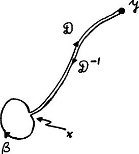
Figure 5: The local consistency condition.

The condition $[U_{\alpha},A_{\varphi}(y)]=0$ for all null homotopic loops can be rewritten in terms of the curvature $F$. For a curve ${{D}}$ joining $x$ and $y$ we define the operator $A_{\varphi}^{{D}}$ on $G_{x}$ by the expression $U_{{D}}^{-1}A_{\varphi}(y)U_{{D}}$. $A_{\varphi}^{{D}}$ maps $G_{x}$ into $G_{x}$ and obviously fulfils the relation

$$\langle\psi_{B}^{{D}}|A_{\varphi}(y)|\psi_{B}^{{D}}\rangle=\langle\psi_{B}|A_{\varphi}^{{D}}|\psi_{B}\rangle.$$ (20)

Now we consider a closed loop $\beta$ at $x$. $\alpha={{D}}\circ\beta\circ{{D}}^{-1}$ is a closed loop at $y$, see Fig. 5. The consistency condition $[U_{\alpha},A_{\varphi}(y)]=0$ can be rewritten as $[U_{\beta},A_{\varphi}^{{D}}]=0$. If we now consider the case of an infinitesimal closed loop $\beta$ at $x$, then the condition finally reads $[F_{\mu\nu}(x),A_{\varphi}^{{{D}}}]=0$, cf. Eq. (14). The curvature tensor at $x$ has to commute with all observables parallel-transported to $x$ along arbitrary curves.

Assume that an observer $B$ at $x\in M$ wants to give a description of measurements performed in a remote space-time region $U\subset M$. We assume that $U$ is contractible. Then there is a map

$$h\,:\,U\times I\,\rightarrow\,M,$$ (21)

where $I=[0,1]$, with the property that $h(y,0)=y$, $h(y,1)=x$ for all $y\in U$ (see Fig. 6). Mathematically, $h$ is a homotopy of the inclusion map $\iota_{U}:U\rightarrow M$ and the constant map $c_{x}:U\rightarrow M$, $c_{x}(y)=x$.

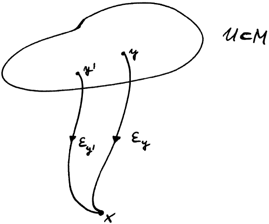
Figure 6: A contraction of $U$ to $x$.

Define the family of curves ${{E}}_{y}$ by ${{E}}_{y}(\tau)=h(y,\tau)$. Thus ${{E}}_{y}$ joins $y$ and $x$. The curves ${{E}}_{y}$ allow us to define a local representation of $U$ at $x$ as follows. Define operators

$$A_{\varphi h}(y)\,{\stackrel{{\scriptstyle def}}{{\displaystyle=}}}\,A_{\varphi{{E}}_{y}}\,{\stackrel{{\scriptstyle def}}{{\displaystyle=}}}\,U_{{{E}}_{y}}\,A_{\varphi}(y)\,U_{{{E}}_{y}}^{-1}\,=\,A_{\varphi}^{{{E}}_{y}^{-1}}.$$ (22)

$A_{\varphi h}(y)$ is an operator on the fibre $G_{x}$. The expectation value for $A$ at $y\in U$, given that $B$’s state vector is $\psi_{B}$, is $\langle\psi_{B}|A_{\varphi h}(y)|\psi_{B}\rangle$. In a local frame, the operators $A_{\varphi{{E}}_{y}|_{\tau}}$ satisfy the equation

$$\partial_{\tau}A_{\varphi{{E}}_{y}|_{\tau}}=[H_{\mu}({{E}}_{\tau})\dot{{{E}}}_{\tau}^{\mu},A_{\varphi{{E}}_{y}|_{\tau}}].$$ (23)

Here ${{D}}|_{\tau}$ is the restriction of the curve ${{D}}:[a,b]\rightarrow M$ to the interval $[a,\tau]$.

4 Applications

In order to develop instructive examples, we study a simple class of systems. We assume that the space-time manifold is a product $M=S\times T$ of a ‘space’ manifold $S$ and a one-dimensional ‘time’ manifold $T$. The bundle under consideration is a trivial bundle $G=M\times{{H}}$. A point in $G$ is of the form $(\vec{x},t,\psi)$, where $\vec{x}\in S$, $t\in T$, $\psi\in{{H}}$. Let $t_{0}\in T$ be a fixed instant of time. Define $S_{t}=S\times\{t\}$, and in particular $S_{0}=S_{t_{0}}$. We assume that there are fields $F_{i}(\vec{x})$ defined on $S_{0}$ fulfilling

$$[F_{i}(\vec{x}),F_{i}(\vec{y})]=0$$ (24)

for $\vec{x}\neq\vec{y}$. $i$ is an index labelling different fields. The parallel transport generators $H_{\mu}$ are assumed to have the following property:

$$[H_{\mu}(\vec{x},t),F_{i}(\vec{y})]=\lambda_{i\mu}^{j}(\vec{x},t,\vec{y})F_{j}(\vec{y}),$$ (25)

where the $\lambda_{i\mu}^{j}(\vec{x},t,\vec{y})$ are complex numbers. Now consider the one-parameter set of operators $F_{i{{E}}|_{\tau}}=U_{{{E}}|_{\tau}}F_{i}(\vec{y})U_{{{E}}|_{\tau}}^{-1}$, where ${{E}}$ is a curve with starting point $(\vec{y},t_{0})$. $F_{i{{E}}|_{\tau}}$ is a solution of the equation

$$\partial_{\tau}F_{i{{E}}|_{\tau}}=[H_{\mu}({{E}}_{\tau})\dot{{{E}}}_{\tau}^{\mu},F_{i{{E}}|_{\tau}}].$$ (26)

We assume ${{E}}$ to be fixed. In order to solve this equation explicitly we make the ansatz

$$F_{i{{E}}|_{\tau}}\,=\,g_{i}^{j}(\tau)\,F_{j}(\vec{y}),\quad g_{i}^{j}(0)=\delta_{i}^{j}.$$ (27)

Inserting the ansatz into Eq. (26) and making use of Eq. (25), we obtain

$$\partial_{\tau}g_{i}^{j}(\tau)\,=\,g_{i}^{l}(\tau)\,\lambda_{l\mu}^{j}({{E}}_{\tau},\vec{y})\,\dot{{{E}}}_{\tau}^{\mu}.$$ (28)

This is an ordinary differential equation for the matrices $g_{i}^{j}(\tau)$. The solution will be denoted by $g_{{{E}}|_{\tau}i}^{j}$. The solution for $F_{i{{E}}|_{\tau}}$ is then $F_{i{{E}}|_{\tau}}=g_{{{E}}|_{\tau}i}^{j}F_{j}(\vec{y})$. In particular, $F_{i{{E}}}=g_{{{E}}i}^{j}F_{j}(\vec{y})$. Now we consider a closed loop $\beta$ at $x$, where ${{E}}$ is assumed to connect $(\vec{y},t)$ and $x$, see Fig. 7.

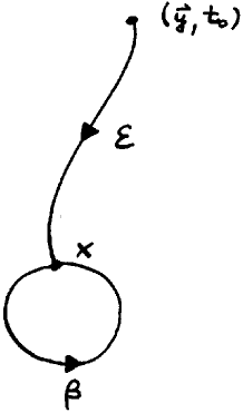
Figure 7: A local symmetry transformation of a field at $(\vec{y},t_{0})$.

Then, in an obvious notation,

$$(F_{i{{E}}})_{\beta}\,=\,F_{i\beta\circ{{E}}}\,=\,g_{\beta\circ{{E}}i}^{j}(\vec{y})\,F_{j}(\vec{y}),$$ (29)

where $g_{\beta\circ{{E}}i}^{j}(\vec{y})=g_{\beta i}^{l}(\vec{y})g_{{{E}}l}^{j}(\vec{y})$, and $g_{{{D}}i}^{j}(\vec{y})$ for a curve ${{D}}:[a,b]\rightarrow M$ satisfies the differential equation

$$\partial_{\tau}g_{{{D}}|_{\tau}i}^{j}(\vec{y})\,=\,g_{{{D}}|_{\tau}i}^{l}(\vec{y})\,\lambda_{l\mu}^{j}({{D}}_{\tau},\vec{y})\,\dot{{{D}}}_{\tau}^{\mu}$$ (30)

with the initial condition $g_{{{D}}|_{a}i}^{j}(\vec{y})=\delta_{i}^{j}$.

Under parallel transport along $\beta$, $F_{i{{E}}}$ is transformed into $g_{\beta i}^{j}(\vec{y})F_{j{{E}}}$. Now assume a homotopy $h$ mapping $U\subset S_{0}$ onto $x$. The representation of the fields $F_{i}$ at $y=(\vec{y},t_{0})$ is $F_{i{{E}}_{y}}$. The transformation of $F_{i{{E}}_{y}}$ depends on $\vec{y}$, namely $(F_{i{{E}}_{y}})_{\beta}=g_{\beta i}^{j}(\vec{y})F_{j{{E}}_{y}}$. Because of this $\vec{y}$-dependence, the transformations are different for every space-time point: they are local.

It can easily be seen that the condition for the matrices $g_{{{E}}i}^{j}$ to be unitary is that

$$\lambda_{j\mu}^{i}=-\overline{\lambda_{i\mu}^{j}}.$$ (31)

If this is the case, an observable $A$ invariant under holonomy transformations can be constructed by $A=\sum_{i}F_{i}^{\dagger}F_{i}$. Since $g_{\beta}^{\dagger}g_{\beta}={1\!\!\!\!\,\,1}$, we obviously have $A_{\beta}=A$.

We now consider two explicit examples. The first one is based on three fields $T_{i}$, $i=1,2,3$ on $M={{R}}^{3}\times{{R}}$. We assume that the $T_{i}$ fulfil the algebra

$$[T_{i}(\vec{x}),T_{j}(\vec{y})]\,=\,i\,{\epsilon_{ij}}^{k}\,T_{k}(\vec{x})\,\delta(\vec{x}-\vec{y}).$$ (32)

The antisymmetric symbol $\epsilon$ is defined by ${\epsilon_{12}}^{3}=(-1)$, $\epsilon_{123}=(+1)$. We define the operators $H_{\mu}$ by

$$H_{\mu}(x)\,=\,-i\,\int_{S_{0}}{\mbox{d}}\vec{z}\,h_{\mu}^{k}(x,\vec{z})\,T_{k}(\vec{z}),$$ (33)

where the $h_{\mu}^{k}(x,\vec{z})$ are real numbers. The commutators of the $H_{\mu}$ with the fields are

$$[H_{\mu}(x),T_{i}(\vec{y})]\,=\,h_{\mu}^{k}(x,\vec{y})\,{\epsilon_{ki}}^{j}\,T_{j}(\vec{y}).$$ (34)

Therefore in this case

$$\lambda_{i\mu}^{j}(x,\vec{y})\,=\,h_{\mu}^{k}(x,\vec{y})\,{\epsilon_{ki}}^{j}.$$ (35)

The condition in Eq. (31) is obviously satisfied. The solutions $g_{{{D}}|_{\tau}i}^{j}(\vec{y})$ of Eq. (30) are therefore $\mbox{SO}(3)$-matrices. For closed curves $\beta$, the parallel transport operator $U_{\beta}$ transforms $T_{i{{E}}_{y}}$ into the $\mbox{SO}(3)$-rotated field $g_{\beta i}^{j}(\vec{y})T_{j{{E}}_{y}}$. If we moreover assume that the $h_{\mu}^{k}(x,\vec{z})$ are $\vec{z}$-independent, i.e.

$$H_{\mu}(x)=-ih_{\mu}^{k}(x)\int_{S_{0}}{\mbox{d}}\vec{z}\,T_{k}(\vec{z}),$$ (36)

then the rotation matrices $g_{\beta i}^{j}(\vec{y})$ are $\vec{y}$-independent; the symmetry is global.

In the second example we assume that the space-time manifold is a torus $M={{R}}^{d-1}\times S^{1}$; this manifold possesses closed timelike curves. We assume fields $q_{i}(\vec{x})$, $i=1,2$, fulfilling

$$[q_{i}(\vec{x}),q_{j}(\vec{y})]=0$$ (37)

and assume that there are conjugated momenta $p_{i}(\vec{x})$ such that

$$[p_{i}(\vec{x}),q_{j}(\vec{y})]=-i\,\delta_{ij}\,\delta(\vec{x}-\vec{y}).$$ (38)

The generators $H_{\mu}$ are defined by

$$H_{\mu}(x)=\frac{1}{2}\,i\,\left[\,\int_{S_{0}}{\mbox{d}}\vec{z}\,h_{\mu}(x,\vec{z})\left(p_{1}(\vec{z})q_{2}(\vec{z})-p_{2}(\vec{z})q_{1}(\vec{z})\right)\,+\,\mbox{h.c.}\right].$$ (39)

They satisfy the equation

$$[H_{\mu}(x),q_{i}(\vec{y})]\,=\,h_{\mu}(x,\vec{y})\,{\epsilon_{i}}^{j}\,q_{j}(\vec{y}).$$ (40)

$\epsilon$ is the antisymmetric symbol with ${\epsilon_{1}}^{2}=1$. Here $\lambda_{i\mu}^{j}(x,\vec{y})=h_{\mu}(x,\vec{y}){\epsilon_{i}}^{j}$. The matrices $g_{{{D}}|_{\tau}i}^{j}(\vec{y})$ are $\mbox{SO}(2)\cong\mbox{U}(1)$-matrices; they simply rotate the fields $q_{1}$, $q_{2}$ into each other. Finally we consider the particularly simple case of quantum mechanics on a closed timelike curve. We set $d=1$, thus reducing the space manifold $S$ to a single point. A closed curve $\alpha$ starting and ending in $T_{0}\in S^{1}$ can, up to homotopy transformations, be classified by its winding number $n\in{{Z}}$. Let

$$g=\left(\begin{array}[]{cc}\cos\theta&\sin\theta\\ -\sin\theta&\cos\theta\end{array}\right)$$ (41)

be the $2\times 2$-matrix corresponding to a parallel transport of $q_{1}$ and $q_{2}$ around a closed curve with winding number $1$. The corresponding transformation for a curve with winding number $n$ is $g^{n}$. If $\theta=2\pi m$, $m\in{{Z}}$, then $g={1\!\!\!\!\,\,1}$. If $\theta=2\pi q$, with $q$ being a rational number, but not an integer, then the set $\{g^{n}\}$ is isomorphic to one of the groups ${{Z}}_{l}$, $l\in{{N}}$, $l>1$. If $\theta=2\pi r$, r being an arbitrary irrational number, then the set $\{g^{n}\}$ is dense in $\mbox{U}(1)$.

5 Summary and Conclusions

In this paper we have developed a geometric formulation of quantum theory on a space-time manifold. The evolution of the state vector is formulated as a parallel transport along the observer’s worldline in a vector bundle over the space-time manifold. A non-trivial holonomy group of the corresponding connection can be viewed as a local symmetry group since the parallel transport of state vectors (or observables) along closed loops should leave expectation values invariant.

The evolution of the state vector is given by a Schrödinger equation and therefore always unitary. This may offer the possibility to formulate a consistent unitary quantum field theory in the presence of closed timelike curves, where the standard formulation fails [4, 5, 6].

Holonomies arise in the case of quantum systems in a different situation as well. A quantum system can acquire a non-trivial Berry phase [7, 8] (or one of its non-Abelian generalizations, see [9, 10]) if, in the case of adiabatic time evolution, its parameters are changed from the outside. In this case time evolution is described by a Hamiltonian $H(\vec{\lambda}(t))$, where $\vec{\lambda}(t)$ denotes the set of external time-dependent parameters. Under certain circumstances, a Berry phase is an observable quantity. In the theory developed in this paper the situation is different. The objects describing the time evolution are the generators of the parallel transport operators themselves. The non-trivial phase is acquired if the point of description of the system is parallel-transported along a closed curve in space-time, not in a parameter space. And, finally, the phase is not observable. Precisely because of the latter property the non-trivial holonomy gives rise to a symmetry.

Open questions are related to the following issues.

• We assumed that the generators $H_{\mu}$ of the parallel transport operators and the representation $\varphi$ of the set of observables were given a priori. In order to study realistic models, the $H_{\mu}$ should be derived from some basic principle. It would certainly be desirable to make contact with Lagrangian field theories.

• The theory was formulated as a way of describing a quantum field, say, in a background space-time. A similar description, however, is applicable for a quantum system located in a small region of space being moved around in space-time. The corresponding parallel transport operators are then active transformations.

• The measurement process must also be formulated consistently. The possibility of a non-trivial ‘twisted’ bundle $\pi_{G}:G\rightarrow M$ may be important here.

• So far only scalar observables have been considered. The theory can easily be extended to vector observables by considering bundles $\pi_{G^{\prime}}:G^{\prime}\rightarrow TM$ over the tangent bundle of $M$. Similarly tensor and spinor objects can be treated. In the cases just mentioned a new structure has to be constructed: that of state transformations at a point, connecting the state vectors of observers whose coordinate systems are related by general coordinate transformations.

• A further complication arises if the Unruh effect is taken into account: accelerated observers will register events even if the system is in the vacuum state [11]. The formalism would have to be extended to mixed states, and the set of states would be a bundle over the jet bundle of $M$, thus allowing us to take into account higher derivatives of the observer’s worldline (i.e. the observer’s acceleration).

• We have interpreted the holonomy group as a group of local symmetry transformations. A very interesting question is whether this local symmetry can in general be related to a gauge symmetry acting on internal degrees of freedom.

• A final remark concerns the use of a classical background space-time. A similar formulation of quantum theory should be possible as soon as the ‘background structure’ admits the geometric objects used in this paper, i.e. bundles and parallel transport operators. This remark may apply to non-commutative structures [12] and to quantum spaces [13], but also to quantum sets [14] and to algebraic and geometric lattices.

Acknowledgements

I wish to thank L. Alvarez-Gaumé, R. Haag and E. Verlinde for conversations and for constructive criticism. Moreover I am grateful to the organizers of the Ringberg workshop in 1994 on ‘Space, Time and Quantum Theory’ for creating a pleasant and fruitful atmosphere for discussions and for the exchange of ideas beyond standard concepts in fundamental physics.

References

- [1]
- [1] N.D. Birrell, P.C.W. Davies, Quantum Field Theory in Curved Space, Cambridge University Press, Cambridge (1982)
- [2] S. Mandelstam, Phys. Rev. D19 (1979) 2391
- [3] S. Kobayashi, K. Nomizu, Foundations of Differential Geometry, John Wiley & Sons, New York (1963)
- [4] J.L. Friedman, N.J. Papastamatiou, J.J. Simon, Phys. Rev. D46 (1992) 4456
- [5] D. Boulware, Phys. Rev. D46 (1992) 4421
- [6] H.D. Politzer, Phys. Rev. D46 (1992) 4470
- [7] M.V. Berry, Proc. R. Soc. Lond. A392 (1984) 45
- [8] B. Simon, Phys. Rev. Lett. 51 (1983) 2167
- [9] F. Wilczek, A. Zee, Phys. Rev. Lett. 52 (1984) 2111
- [10] G. Papadopoulos, J. Phys. A25 (1992) 2071
- [11] W.G. Unruh, Phys. Rev. D14 (1976) 870
- [12] R. Coquereaux, Noncommutative Geometry and Theoretical Physics, CPT-88/P-2147 (1988)
- [13] J. Wess, B. Zumino, Nucl. Phys. Proc. Suppl. 18B (1991) 302
- [14] D. Finkelstein, Quantum Set Theory and Geometry, in Quantum Theory and the Structures of Time and Space, Vol. 4, eds. L. Castell, M. Drieschner, C.F. v. Weizsäcker, Carl Hanser Verlag, München, Wien (1981)