Spin Dynamics of the LAGEOS Satellite in Support of a Measurement of the Earth’s Gravitomagnetism

Abstract

LAGEOS is an accurately-tracked, dense spherical satellite covered with 426 retroreflectors. The tracking accuracy is such as to yield a medium term (years to decades) inertial reference frame determined via relatively inexpensive observations. This frame is used as an adjunct to the more difficult and data intensive VLBI absolute frame measurements. There is a substantial secular precession of the satellite’s line of nodes consistent with the classical, Newtonian precession due to the non-sphericity of the earth. Ciufolini has suggested the launch of an identical satellite (LAGEOS-3) into an orbit supplementary to that of LAGEOS-1: LAGEOS-3 would then experience an equal and opposite classical precession to that of LAGEOS-1. Besides providing a more accurate real-time measurement of the earth’s length of day and polar wobble, this paired-satellite experiment would provide the first direct measurement of the general relativistic frame-dragging effect. Of the five dominant error sources in this experiment, the largest one involves surface forces on the satellite, and their consequent impact on the orbital nodal precession. The surface forces are a function of the spin dynamics of the satellite. Consequently, we undertake here a theoretical effort to model the spin ndynamics of LAGEOS. In this paper we present our preliminary results.

I The LAGEOS-3 Mission.

The Laser Geodynamic Satellite Experiment (LAGEOS-3) is a joint USAF, NASA, and ASI proposed program to measure, for the first time, a quasi-stationary property of the earth – its gravitational magnetic dipole moment (gravitomagnetism) as predicted by Einstein’s theory of general relativity. This gravitomagnetic field causes local inertial frames to be dragged around with the earth at a rate proportional to the angular momentum of the earth, and inversely proportional to the cube of the distance from the center of the earth. Thus the line of nodes of the orbital plane of LAGEOS-3 precesses eastward at $32\ mas/yr$. Although in this example the frame dragging effect is small compared to the torque on the orbital plane due to the oblateness of the earth, it is an essential ingredient in the dynamics of accretion disks, binary systems, and other astrophysical phenomena [1].

Today, almost eighty years after Einstein introduced his geometric theory of gravity, we have just begun to measure – to verify – his gravitation theory. Of no less stature than the “tide producing” $-M/r^{2}$ “electric component” of gravity is the inertial-frame defining “magnetic component” of gravitation $-J/r^{3}$. To see this force in action: first, inject a satellite into a polar orbit about an earth-like mass idealized as not spinning with respect to the distant quasars. The satellite will remain in orbit in a continuous acceleration towards the center-of-mass of the attracting body under the influence of the Newtonian $1/r^{2}$ force, and its orbital plane will remain fixed in orientation with respect to distant quasars. Second, spin the central body, giving it angular momentum, and follow the trajectory of the satellite. Its orbital plane will experience a torque along the central body’s rotation axis. The orbital plane will undergo a precessional motion in the direction of the central body’s rotation. The mass in motion of the central body, or “mass current”, produces a dipole gravitational field – the gravitomagnetic field. In the case of a satellite orbiting at two earth radii, the orbital plane will precess about the body axis of the earth at approximately $32\ mas/yr$. This is the Lense-Thirring effect [2].

The Lense-Thirring force has never been directly measured. A measurement of this gravitomagnetic force can be compared to the pioneering work of Michael Faraday on the measurement of the magnetic force between two current-carrying wires. However, the laboratory setting for this gravity measurement will be the 4-dimensional curved spacetime (approximately Kerr) geometry enveloping the earth. The idea behind the LAGEOS gravity measurement is simple. Whereas the Everitt-Fairbanks experiment (Gravity Probe-B) proposes putting a gyroscope into polar orbit [3], the Ciufolini LAGEOS-3/LAGEOS-1 experiment [4] proposes the use of the orbital planes themselves as a gyroscope.

In 1976 NASA launched the LAGEOS-1 satellite, a totally passive $60~{}cm$ diameter ball of aluminum with $426$ retro-reflecting mirrors embedded in its surface. (There are numerous globally-located laser tracking stations to observe LAGEOS-type satellites.) LAGEOS-1 was injected into a two earth-radii circular orbit at an inclination of $110~{}\deg$. Due to the oblateness of the earth, the orbital plane rotates at a rate of $126~{}\deg/yr$. This torquing can only be modeled to $450~{}mas/yr$ – which is not accurate enough to measure the $32~{}mas/yr$ gravitomagnetic force. The idea of Ciufolini is to launch another LAGEOS satellite (LAGEOS-3) into an orbit identical to that of LAGEOS-1, except that its inclination is supplementary ($70~{}\deg=180~{}\deg-110~{}\deg$). This proposed orbital plane will rotate in the opposite direction, i.e., $-126~{}\deg/yr$. The intersection of the two (LAGEOS-1, LAGEOS-3) orbital planes will sweep out a “tandem-generated gyro plane” (Fig. 1). The utilization of two satellites cancels out many of the large precessional effects due to mass eccentricities of the earth, providing a plane inertial enough for a measurement, accurate to five percent (or better), of the “magnetic component” of gravity.

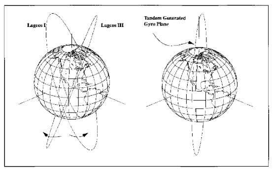
FIG. 1.: The tandem-generated gyro plane and the LAGEOS-3 satellite experiment. Both the Gravity Probe B (GP-B) experiment at Stanford and the LAGEOS-3 experiment share the feature of generating an effective polar orbit so as to cancel the torque on the orbital plane arising from the oblateness of the earth. In the case of the GP-B experiment, a drag-free superconducting gyroscope is launched into a polar orbit. In the case of the LAGEOS-3 experiment, a satellite is launched into an inclination that is supplementary ($70=180-110~{}\deg$) to the LAGEOS-1 satellite. As the orbital planes precess in equal and opposite directions, the line of intersection of these two supplementary planes evolves so as to sweep out a polar plane. Einstein’s theory of general relativity predicts that this tandem-generated gyroplane will precess at a rate of $32~{}mas/yr$. In the GP-B case, the gyroscope is $\sim cm$ in diameter, while it is $12,271.79~{}km$ in diameter for LAGEOS.

II Why Spin Dynamics?

The success of the LAGEOS experiment hinges upon the detection of a $32~{}mas/yr$ eastward drift of the line of nodes of the two satellites. A strong effort is now underway to model the orbital and spin dynamics of these satellites, and to make an assessment of the uncertainties these will add to the desired measurements. Encapsulated in Table I are the five major classes of errors in this experiment: (1) geopotential (other than even zonals) and tides, (2) earth radiation pressure, (3) uncertainty in other relativistic effects, (4) earth and solar-induced thermal forces, and (5) even zonal geopotentials (per $0.1\deg$ inclination injection error). Due to the recent GEM-T1 improvements in the earth’s zonal harmonics, the errors due to solid-earth tides have been significantly reduced, and are now potentially smaller than those due to surface effects [5].

These surface effects (e.g., Yarkowsky thermal drag, neutral and charged particle drag) cause a change in the nodal precession of the satellite, thus contributing to what will be potentially the largest source of error in the LAGEOS-3 measurement of the gravitomagnetic effect. In modeling these surface forces, in particular the Yarkowsky thermal drag (also referred to as the Rubincam effect) due to the satellite’s differential heating and delayed reradiation, the behavior of the spin vector of the satellite is of crucial importance. That the uncertainties induced by the surface forces on LAGEOS are on the order of 4%, out of a 6% experiment, makes such a theoretical modeling of paramount importance. With this in mind, we undertake in this paper a theoretical model of the spin dynamics of LAGEOS-type satellites, and compare our results with observational data.

We must emphasize that we are looking for qualitative, not quantitative, results. We do not intend to predict the exact magnitude and direction of the spin vector at any particular instant. Instead, we desire a rough estimate of its magnitude, and whether its behavior is predictable or chaotic. We seek to answer questions of the sort: “In the asymptotic limit, does the satellite tidally lock, tumble, or have some other behavior?”

Previous studies of the spin dynamics of the LAGEOS-1 satellite [7] were valid only for spin rates much larger than the orbital frequency. Today, however, the spin of the satellite, decaying with a three-year time constant, is rapidly approaching the orbital period. We therefore require an analysis in the low–frequency regime. Unlike the earlier analysis which dealt with orbit-averaged quantities, we will solve numerically the full set of dynamical equations. As we will show, while the low frequency regime exhibits complex behavior, the asymptotic state of this forced, damped system appears to be tidally locked. In this paper we will examine the spin-orbit resonance phase and discuss the asymptotic state of the spin of the satellite. It is the goal of this research to provide an optimum strategy for the measurement of the spin dynamics of the LAGEOS satellites in support of the proposed gravity measurement. In addition, we use our theoretical model to propose an optimum orbital injection procedure for LAGEOS-3: it is our opinion that the LAGEOS-3 satellite should be injected into the orbital plane with as large a spin rate as possible. Our results provide the first analysis of the asymptotic spin dynamics of the LAGEOS satellite. Previous calculations were unable to analyze the spin-orbit resonances of the satellite, nor its asymptotic behavior, which will play a crucial role in the experiment. We demonstrate in this paper that the LAGEOS-1 satellite will be sufficiently predictable to support the gravitomagnetic measurement.

Geopotential and tides	2%
Earth radiation pressure	1%
Uncertainty in other relativistic effects	1%
Thermal forces	1-3%
Even zonal geopotential	$<$1%
Random and stochastic errors	2%
RSS error	3-4%

TABLE I.: The latest error budget for the LAGEOS-3 Lense-Thirring experiment. Errors in geopotential and tides reflect improvement over GEM-T1. Uncertainty in the thermal forces depends mainly on knowledge of spin-axis motion. The even zonal geopotential error calculation assumes less than $0.03~{}\deg$ inclination injection error. The random and stochastic error estimate can accommodate seasonal variations in low degree spherical harmonics of the geopotential.

III Modeling the Spin

It is rather interesting that after 36 years the spin dynamics of passive satellites is once again important to the field of astrodynamics. In 1957 Vinti [8] analyzed the spin dynamics of a non-ferromagnetic spherical satellite in the earth’s magnetic field, which was then of critical importance to the alignment of antennas. Today we perform the same analysis on a slightly oblate satellite, of critical importance to the first measurement of the magnetic component of gravity, as predicted by Einstein.

There are many factors to consider when analyzing the spin dynamics of an oblate, metallic satellite orbiting in the gravitational and magnetic fields of the earth. The most prominent effect is the torqueing due to the gravitational field of the earth. This arises from the oblateness of the satellite, with the oblateness of the earth producing a negligible contribution that can be added to our calculations as an adiabatic correction. If the satellite’s (bulging) equatorial plane lies in the plane of orbit, no such torques are possible. However, when the satellite is not placed exactly in such a position, gravitational torques will arise. In an effort to model these torques, we consider the situation of an oblate spheroid in orbit around a point mass. As was done by Bertotti and Iess, we parallel the development in Goldstein [9].

Bertotti and Iess’s analysis of the effects of gravity on the spin dynamics of the oblate satellite, which resulted in predicting a chaotic spin dynamics of arbitrarily large amplitude in the obliquity at late times, is not appropriate for small rates of spin. Their prediction is based on the “Hipparcos” formula for the rate of precession $\omega_{p}$ of an oblate satellite in the inhomogeneous gravity field of the earth

$$\omega_{p}={3\over 2}\,\Delta\,{\omega_{0}^{2}\over\omega_{3}}\cos\theta,$$ (1)

where $\omega_{0}$ is the orbital angular velocity, $\omega_{3}$ is the satellite spin rate, $\theta$ is the obliquity angle of the satellite (the angle between $\vec{\omega}$ and the normal to the orbital plane) and

$$\Delta={I_{3}-I_{1}\over I_{3}}$$ (2)

is the satellite’s oblateness. Here $I_{3}$ and $I_{1}=I_{2}$ are the principal moments of inertia (the principal direction corresponding to $I_{3}$ is assumed to be that of $\vec{\omega}$ and coincides, by assumption, with the symmetry axis of the oblate satellite).

It is argued by Bertotti and Iess that, since $\omega_{p}\propto 1/\omega_{3}$, the gravitational precession in the asymptotic limit of small $\omega$ becomes very fast and may make the spin dynamics chaotic. This conclusion is based upon a misunderstanding. We have shown, via a careful analysis of assumptions underlying the “Hipparcos” formula, that even in the approximation commonly used in deriving the formula (averaging of the gravitational potential over the satellite orbit, dipole cutoff of the multipole decomposition, etc.) Eqn. (1) can only be used when

$${6\omega_{0}^{2}\Delta\cos^{2}\theta\over\omega_{3}^{2}}\sim{\omega_{0}^{2}\over\omega_{3}^{2}}\ll 1,$$ (3)

i.e., when the spin rate of the satellite is much greater than its orbital angular velocity. The latter restriction is easy to overcome, and the corrected equation for $\omega_{p}$ is

$$\omega_{p}={1\over 2}{\omega_{3}\over\cos\theta}\left(1-\sqrt{1+{6\omega_{0}^{2}\Delta\cos^{2}\theta\over\omega_{3}^{2}}}\right).$$ (4)

This equation imposes a bound on $|\omega_{p}|$:

$$|\omega_{p}|<\omega_{0}\sqrt{{3\over 2}\Delta},$$ (5)

which makes it clear that the rate of precession cannot grow to cause chaoticity of the satellite spin dynamics. A subsequent qualitative investigation [10] by Chris Fuchs has shown that when magnetic forces are included in the picture the precession rate remains bounded, and should be much smaller than $\omega_{0}$. Another conclusion reached in the course of our analysis has been that, when both gravitational and magnetic forces are taken into account, the nutation, although bounded in its amplitude, does not disappear completely even in the asymptotic limit. The value of these results, however, is limited by the fact that they do not yield the exact bounds, nor do they provide any information on the time scale to reach the asymptotic limit. However, they do clearly show that chaoticity of the LAGEOS spin dynamics caused by an unbounded growth of gravitationally-induced precession cannot occur.

Another important factor governing the evolution of the spin vector is the interaction of the metallic core of the satellite with the magnetic field of the earth. The LAGEOS satellite [11] is composed of two aluminum hemispheres bolted together, with a brass cylindrical core along its body axis (the original axis of spin) (Fig. 2). The spinning of this metallic object in the magnetic dipole field of the earth (and the motion through that field) will cause eddy currents within the satellite, which will in turn cause dissipation through Joule heating and a slowdown of the spin, and furthermore will cause torques on the spin vector. These torques can be understood as the interaction of the magnetic dipole, caused by the induced eddy currents, with the magnetic field of the earth. In modeling this effect, we have treated a uniform, spherical object in the orbit of a perfect magnetic dipole. Here we are concerned with a simple qualitative analysis of the spin dynamics of LAGEOS, as the complexity of the true satellite geometry prohibits us from a precise model of the eddy current distribution. Our theoretical model permits us to analyze arbitrary inclinations of the orbital plane to the earth’s magnetic dipole axis. The results presented in this paper correspond to a retrograde $I=109.86~{}\deg$ orbit.

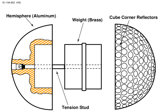
FIG. 2.: A schematic representation of the LAGEOS assembly. The two hemispheres form a $60~{}cm$ diameter sphere and are made of $6061$ aluminum. There are $426$ cube corner reflectors recessed into the satellite’s surface. To obtain the desired surface-to-mass ratio, the inside of the aluminum hemispheres were hollowed out to make room for a brass cylinder of $31.76~{}cm$ diameter and $26.70~{}cm$ height. The LAGEOS-1 satellite was launched June 7, 1976 into an inclination of $109.8585~{}\deg$ and semimajor orbit of $12271.790~{}km$. (This figure is adapted from Ref. [11].)

The problem of a spinning metallic sphere in a constant magnetic field has been treated by Landau and Lifshitz [12], and we avail ourselves of their results. For our purposes, we ignore the torques caused by the changing magnetic field due to the orbit (as opposed to spin) of the satellite. These torques can be shown to be negligible until asymptotically late stages of motion, and have no qualitative effects upon the dynamics.

The source of many of the difficulties in doing analyses of such orbiting, spinning bodies lies in the involved coordinate systems needed to describe their motion. Thus, it is important at this point to give a brief description of the coordinates we will use in this paper. In our analysis of the spin dynamics of the LAGEOS satellite we found it convenient to introduce the following four coordinate systems:

1. The orbit-centered inertial frame (OCI) $\{x_{1},y_{1},z_{1}\}$. Here the $z_{1}$-axis is oriented along the normal to the orbital plane of the satellite ($\sim 70.142\deg$ coinclination). The $x_{1}$-axis is defined to be the intersection of the orbital plane and the earth’s equatorial plane, and the origin is the center of mass of the earth. We have assumed here that this frame is inertial, and have not included the secular drag of the line-of-nodes of the orbital plane due to the oblateness of the earth. This $\sim 126~{}\deg/yr$ precession can be included at the end of our analysis as an adiabatic correction, and again has no qualitative effects upon the dynamics.

2. The earth-centered inertial (ECI) reference frame $\{x_{2},y_{2},z_{2}\}$. Here the $z_{2}$-axis is aligned with the body axis of the earth. The $x_{2}$-axis lies in the earth’s equatorial plane at zero degrees longitude, and the origin coincides with the center of the earth.

3. The body frame (non-inertial) $\{x_{b},y_{b},z_{b}\}$. The origin is at the center of the satellite, and the axes correspond to a set of principal axes. The satellite is assumed to be a slightly oblate ($\sim 3.27\%$) spheroid of brass, and the $z_{b}$-axis is aligned along its body axis. The $x_{b}$ and $y_{b}$ axes are an arbitrary fixed set of orthogonal axes spanning the equatorial plane of the satellite. In our calculations, the body axis is related to the orbit-centered frame through the three Euler angles $\theta$, $\phi$, and $\psi$. The nutation angle $\theta$ is the angle between $z_{b}$ and $z_{1}$, while the angle of precession $\phi$ is the angle between the $x_{1}$-axis and the line of nodes (the intersection of the orbital plane and the equatorial plane of the satellite ($x_{b}$-$y_{b}$ plane)). The spin angle $\psi$ is the angle between the line of nodes and the $x_{b}$-axis.

4. The Landau-Lifshitz (non-inertial) coordinate system $\{x^{ll},y^{ll},z^{ll}\}$. The $z^{ll}$-axis is aligned along the instantaneous angular momentum vector of the satellite ($\vec{\omega}$). The $x^{ll}$-axis is picked so that the instantaneous magnetic field ($\vec{B}$) at the satellite lies in the $x^{ll}-z^{ll}$ plane. Note that $z^{ll}$ need not be aligned with the body axis of the satellite, and in fact, during the asymptotic behavior of the satellite they are vastly different. In particular, the angle ($\xi$) between the symmetry axis of the satellite ($\hat{z}_{b}$) and the instantaneous angular momentum vector ($\hat{z}_{ll}$) can be expressed in terms of the three Euler angles as

$$\sin\xi=\left(1+{I_{3}^{2}\over I_{1}^{2}}{(\dot{\phi}\cos\theta+\dot{\psi})^{2}\over(\dot{\phi}^{2}\sin^{2}\theta+\dot{\theta}^{2})}\right)^{-1/2}$$ (6)

In the early stages of the LAGEOS mission when $\dot{\psi}\gg\dot{\theta}$ and $\dot{\psi}\gg\dot{\phi}$ this angle is rather small ($\bar{\xi}\approx(I_{1}/I_{3})(\bar{\omega}_{\theta}/\omega_{\psi})\approx 6.3516\times 10^{-10}$).

A proper interpretation of the results of the numerical simulation requires a careful distinction between $\omega_{p}$ and $\omega_{\phi}$ (where $\phi$ is the Euler angle of the body frame). The two coincide only under the assumption that the $\omega_{3}$ component of the satellite’s angular velocity is responsible for all of the satellite’s energy, or, to put it differently, the angular momentum of the satellite is directed along the body axis of the satellite. As the satellite’s spinning motion slows down, this last assumption is violated. $\omega_{p}$ represents only a part of $\omega_{\phi}$, the other part being caused by the “tidal locking” effect. As we shall see, this is exactly what happens in the asymptotic phase of the satellite’s motion. Nevertheless, both $\omega_{p}$ and $\omega_{\phi}$ remain bounded.

IV Spin Dynamics of LAGEOS: The Equations.

The spin dynamics are determined by Euler’s equations

$$I_{1}\dot{\omega}_{1}-\omega_{2}\omega_{3}(I_{1}-I_{3}) = N_{1},$$ (7)

$$I_{1}\dot{\omega}_{2}-\omega_{3}\omega_{1}(I_{3}-I_{1}) = N_{2},$$ (8)

$$I_{3}\dot{\omega}_{3} = N_{3},$$ (9)

where $\omega_{1}$, $\omega_{2}$, $\omega_{3}$ are the components of the satellite’s angular velocity in the body frame, $I_{1}=I_{2}$, $I_{3}$ are the principal moments of inertia, and $N_{1}$, $N_{2}$, $N_{3}$ are the components of the torques along the satellite’s principal axes. After substituting the expressions for $\omega_{1}$, $\omega_{2}$, $\omega_{3}$ in terms of the Euler angles

$$\omega_{1} = \dot{\phi}\sin\theta\sin\psi+\dot{\theta}\cos\psi,$$ (10)

$$\omega_{2} = \dot{\phi}\sin\theta\cos\psi-\dot{\theta}\sin\psi,$$ (11)

$$\omega_{3} = \dot{\phi}\cos\theta+\dot{\psi},$$ (12)

the Euler equations become

$$\ddot{\theta} = \ddot{\theta}_{free}+{N_{1}\cos{\psi}-N_{2}\sin{\psi}\over I_{1}},$$ (13)

$$\ddot{\theta}_{free} = \left({I_{1}-I_{3}\over I_{1}}\right)\dot{\phi}^{2}\cos{\theta}\sin{\theta}-{I_{3}\over I_{1}}\dot{\psi}\dot{\phi}\sin\theta,$$ (14)

$$\ddot{\phi} = \ddot{\phi}_{free}+{N_{1}\sin{\psi}+N_{2}\cos{\psi}\over I_{1}\sin{\theta}},$$ (15)

$$\ddot{\phi}_{free} = \left({I_{3}-2I_{1}\over I_{1}}\right){\cos{\theta}\over\sin{\theta}}\dot{\theta}\dot{\phi}+{I_{3}\over I_{1}}{\dot{\theta}\dot{\psi}\over\sin{\theta}},$$ (16)

$$\ddot{\psi} = \ddot{\psi}_{free}+{N_{3}\over I_{1}}-{N_{1}\sin{\psi}+N_{2}\cos{\psi}\over I_{1}}{\cos{\theta}\over\sin{\theta}},$$ (17)

$$\ddot{\psi}_{free} = -\left({I_{3}-I_{1}\over I_{1}}\right){\cos^{2}{\theta}\over\sin{\theta}}\dot{\theta}\dot{\phi}+{\dot{\theta}\dot{\phi}\over\sin{\theta}}-{I_{3}\over I_{1}}{\cos{\theta}\over\sin{\theta}}\dot{\theta}\dot{\psi}.$$ (18)

The torque components $N_{1}$, $N_{2}$, $N_{3}$ are due to gravitational and magnetic forces acting on the satellite

$$N_{i}=N_{i}^{(g)}+N_{i}^{(m)},\quad i=1,2,3.$$ (19)

Gravitational torques in the body frame are given by

$$N_{1}^{(g)} = -\cos\psi{\partial V\over\partial\theta}-{\sin\psi\over\sin\theta}{\partial V\over\partial\phi}+{\cos\theta\sin\psi\over\sin\theta}{\partial V\over\partial\psi},$$ (20)

$$N_{2}^{(g)} = \sin\psi{\partial V\over\partial\theta}-{\cos\psi\over\sin\theta}{\partial V\over\partial\phi}+{\cos\theta\cos\psi\over\sin\theta}{\partial V\over\partial\psi},$$ (21)

$$N_{3}^{(g)} = -{\partial V\over\partial\psi}.$$ (22)

Using the standard dipole approximation, the gravitational potential $V$ is

$$V={GM(I_{3}-I_{1})\over 2R^{3}}\left(3\gamma^{2}-1\right),$$ (23)

where $\gamma$ is the direction cosine between (1) the radial vector from the satellite center of mass to the center of the earth, and (2) the symmetry axis of the satellite. It is related to Euler’s angles via

$$\gamma=\sin\theta\sin(\eta-\eta_{0}-\phi),$$ (24)

where $\eta$ gives the angular position of the center of mass of the satellite in its orbit about the earth, and $\eta_{0}$ is an arbitrary starting position. The potential is given by

$$V={GM(I_{3}-I_{1})\over 2R^{3}}\left(3\sin^{2}\theta\sin^{2}(\eta-\eta_{0}-\phi)-1\right),$$ (25)

and thus

$$-{\partial V\over\partial\theta} = -{3GM(I_{3}-I_{1})\over R^{3}}\sin\theta\cos\theta\sin^{2}(\eta-\eta_{0}-\phi),$$ (26)

$$-{1\over\sin\theta}{\partial V\over\partial\phi} = {3GM(I_{3}-I_{1})\over R^{3}}\sin\theta\sin(\eta-\eta_{0}-\phi)\cos(\eta-\eta_{0}-\phi),$$ (27)

$${\partial V\over\partial\psi} = 0.$$ (28)

Equations (10) and (14) lead to the following final expressions for the components of the gravitational torque in the body frame

$$N^{(g)}_{1} = {3GM(I_{3}-I_{1})\over R^{3}}\sin\theta\sin(\eta-\eta_{0}-\phi)\left\{\begin{array}[]{c}-\cos\theta\cos\psi\sin(\eta-\eta_{0}-\phi)\\ +\sin\psi\cos(\eta-\eta_{0}-\phi)\end{array}\right\},$$ (31)

$$N^{(g)}_{2} = {3GM(I_{3}-I_{1})\over R^{3}}\sin\theta\sin(\eta-\eta_{0}-\phi)\left\{\begin{array}[]{c}\cos\theta\sin\psi\sin(\eta-\eta_{0}-\phi)\\ +\cos\psi\cos(\eta-\eta_{0}-\phi)\end{array}\right\},$$ (34)

$$N^{(g)}_{3} = 0.$$ (35)

As for the magnetic effects, we are interested in the torque components acting on a conducting ball of radius $a$ spinning with angular velocity $\vec{\omega}$ in an external magnetic field $\vec{B}$. We take our expressions from Landau and Lifshitz [12], noting that their results are for what we have dubbed the Landau-Lifshitz frame (as described above), and for our purposes need to be transformed to the body frame.

As already described, the Landau-Lifshitz frame is determined by the vectors $\vec{\omega}$ and $\vec{B}$. If we introduce an arbitrary set of rectangular coordinates $x$, $y$, $z$, in this frame $\vec{\omega}$ and $\vec{B}$ are represented as

$$\vec{\omega} = \omega_{x}\,\hat{x}+\omega_{y}\,\hat{y}+\omega_{z}\,\hat{z}=\langle\omega_{x},\omega_{y},\omega_{z}\rangle,$$ (36)

$$\vec{B} = B_{x}\,\hat{x}+B_{y}\,\hat{y}+B_{z}\,\hat{z}=\langle B_{x},B_{y},B_{z}\rangle,$$ (37)

where hats ($\hat{x}$) denote vectors normalized to unity. The transition between this arbitrary frame and the Landau-Lifshitz frame is given by

$$\left(\begin{array}[]{c}\hat{x}^{ll}\\ \hat{y}^{ll}\\ \hat{z}^{ll}\end{array}\right)=\left(\begin{array}[]{ccc}[(\vec{\omega}\times\vec{B})\times\vec{\omega}]_{x}\over\omega|\vec{\omega}\times\vec{B}|&[(\vec{\omega}\times\vec{B})\times\vec{\omega}]_{y}\over\omega|\vec{\omega}\times\vec{B}|&[(\vec{\omega}\times\vec{B})\times\vec{\omega}]_{z}\over\omega|\vec{\omega}\times\vec{B}|\\ (\vec{\omega}\times\vec{B})_{x}\over|\vec{\omega}\times\vec{B}|&(\vec{\omega}\times\vec{B})_{y}\over|\vec{\omega}\times\vec{B}|&(\vec{\omega}\times\vec{B})_{z}\over|\vec{\omega}\times\vec{B}|\\ \omega_{x}\over\omega&\omega_{y}\over\omega&\omega_{z}\over\omega\end{array}\right)\,\left(\begin{array}[]{c}\hat{x}\\ \hat{y}\\ \hat{z}\end{array}\right),$$ (38)

where $\omega=|\vec{\omega}|$.

The components of the magnetic torque in the Landau-Lifshitz frame are given by

$$N^{ll}_{x} = V\alpha^{\prime\prime}B^{ll}_{x}B^{ll}_{z},$$ (39)

$$N^{ll}_{y} = -V\alpha^{\prime}B^{ll}_{x}B^{ll}_{z},$$ (40)

$$N^{ll}_{z} = -V\alpha^{\prime\prime}(B^{ll}_{x})^{2},$$ (41)

where $V=4\pi a^{3}/3$ is the volume of the ball, $B^{ll}_{x}$, $B^{ll}_{y}$, $B^{ll}_{z}$ are components of the magnetic field in the Landau-Lifshitz frame, and the real and complex parts of the coefficient of magnetization are

$$\alpha^{\prime} = -{3\over 8\pi}\left[1-{3\delta\over 2a}{{\rm sinh}\left(2{a\over\delta}\right)-\sin\left(2{a\over\delta}\right)\over{\rm cosh}\left(2{a\over\delta}\right)-\cos\left(2{a\over\delta}\right)}\right],$$ (42)

$$\alpha^{\prime\prime} = -{9\delta^{2}\over 16\pi a^{2}}\left[1-{a\over\delta}{{\rm sinh}\left(2{a\over\delta}\right)+\sin\left(2{a\over\delta}\right)\over{\rm cosh}\left(2{a\over\delta}\right)-\cos\left(2{a\over\delta}\right)}\right],$$ (43)

with

$$\delta={c\over\sqrt{2\pi\sigma\omega}}.$$

Here $c$ is the speed of light and $\sigma$ is the specific conductivity of the material forming the ball. At small values of $\omega$ ($\delta\gg a$), $\alpha^{\prime}$ and $\alpha^{\prime\prime}$ can be approximated by the expressions

$$\alpha^{\prime} \approx -{4\pi\over 105}{a^{4}\sigma^{2}\omega^{2}\over c^{4}},$$ (44)

$$\alpha^{\prime\prime} \approx {a^{2}\sigma\omega\over 10c^{2}}.$$ (45)

Components of the magnetic field can be evaluated in the ECI frame using the dipole approximation. In the spherical coordinate representation of the ECI frame, the magnetic field components are

$$B_{r_{1}} = -{2M\over R^{3}}\cos\theta_{1},$$ (46)

$$B_{\theta_{1}} = -{M\over R^{3}}\sin\theta_{1},$$ (47)

$$B_{\phi_{1}} = 0,$$ (48)

where $M$ is the magnetic dipole moment of the earth. In the rectangular coordinate representation of the ECI frame (the index 1 is used everywhere for quantities in ECI)

$$B_{x_{1}} = B_{r_{1}}\sin\theta_{1}\cos\phi_{1}+B_{\theta_{1}}\cos\theta_{1}\cos\phi_{1},$$ (49)

$$B_{y_{1}} = B_{r_{1}}\sin\theta_{1}\sin\phi_{1}+B_{\theta_{1}}\cos\theta_{1}\sin\phi_{1},$$ (50)

$$B_{z_{1}} = B_{r_{1}}\cos\theta_{1}-B_{\theta_{1}}\sin\theta_{1}.$$ (51)

Transforming these to the OCI frame:

$$B_{x_{2}} = (B_{r_{1}}\sin\theta_{1}+B_{\theta_{1}}\cos\theta_{1})\cos\phi_{1},$$ (52)

$$B_{y_{2}} = (B_{r_{1}}\sin\theta_{1}+B_{\theta_{1}}\cos\theta_{1})\sin\phi_{1}\cos\xi+(B_{r_{1}}\cos\theta_{1}-B_{\theta_{1}}\sin\theta_{1}),\sin\xi$$ (53)

$$B_{z_{2}} = -(B_{r_{1}}\sin\theta_{1}+B_{\theta_{1}}\cos\theta_{1})\sin\phi_{1}\sin\xi+(B_{r_{1}}\cos\theta_{1}-B_{\theta_{1}}\sin\theta_{1})\cos\xi,$$ (54)

where $\xi$ is the colatitude angle of the orbit with respect to magnetic north, and the index 2 is used for quantities in the OCI. The satellite’s semimajor axis is $R=1.227179\times 10^{9}~{}cm$, and for the earth’s magnetic dipole moment we used $M=7.9\times 10^{25}~{}G-cm^{3}$. Although we do not average the magnetic field in our simulations, it was useful for back of the envelope calculations to note that the the magnetic field, averaged over one orbit, is $|\bar{B}|=0.155814~{}G$, with components,

$$\bar{B}_{x_{2}} = 0~{}G,$$ (55)

$$\bar{B}_{y_{2}} = -0.0388558~{}G,$$ (56)

$$\bar{B}_{z_{2}} = -0.150891~{}G.$$ (57)

The angles $\theta_{1}$ and $\phi_{1}$ are dependent upon the satellite’s position in its orbit. The satellite’s coordinates in the OCI frame are

$$x_{2} = r\cos(\eta-\eta_{0}),$$ (58)

$$y_{2} = r\sin(\eta-\eta_{0}),$$ (59)

$$z_{2} = 0,$$ (60)

where

$$\eta=-{2\pi\over T_{\rm orbit}}t.$$ (61)

In ECI we have

$$x_{1} = R\cos(\eta-\eta_{0}),$$ (62)

$$y_{1} = R\sin(\eta-\eta_{0})\cos\xi,$$ (63)

$$z_{1} = -R\sin(\eta-\eta_{0})\sin\xi.$$ (64)

Hence,

$$\sin\theta_{1} = \sqrt{\cos^{2}(\eta-\eta_{0})+\sin^{2}(\eta-\eta_{0})\cos^{2}\xi},$$ (65)

$$\cos\theta_{1} = -\sin(\eta-\eta_{0})\sin\xi,$$ (66)

$$\cos\phi_{1} = {\cos(\eta-\eta_{0})\over\sin\theta_{1}},$$ (67)

$$\sin\phi_{1} = {\sin(\eta-\eta_{0})\cos\xi\over\sin\theta_{1}}.$$ (68)

The three Euler equations (Eq. 18), with the magnetic and gravitational torques included (properly transformed to the body frame), give us the vehicle to analyze qualitatively the spin dynamics of the LAGEOS-1 satellite. We present our results from the numerical integration of these equations in the following two sections.

V Initial-Value Data.

We solved the Euler equations (Eq. 18) using a fourth-order Bulirsch-Stoer algorithm with adaptive time-stepping [13]. The equations were integrated for $3\times 10^{9}$ seconds, as we wanted to (1) reproduce the experimentally-measured spin rates ($17~{}yrs$ following launch), (2) examine the spin-orbit resonance ($\sim 27~{}yrs$ after launch), and (3) reveal the asymptotics of the spin dynamics ($\sim 79+yrs$ after launch). The experimentally-measured exponential decrease in the spin rate imposed a constraint on our theoretical model, linking the “effective” radius of the satellite ($a$) with the satellite’s “effective” conductivity ($\sigma$):

$$\sigma a^{5}\sim 1.19552\times 10^{24}~{}cm^{5}/s.$$ (69)

The satellite was modeled as a $25.55~{}cm$ radius spheroid of brass ($\sigma=1.098\times 10^{17}~{}s^{-1}$). LAGEOS I’s moment of inertia about the body axis is $I_{z_{b}}=1.314\times 10^{8}~{}g-cm^{2}$, while the moment of inertia perpendicular to the body axis is $I_{x_{b}}=I_{y_{b}}=1.271\times 10^{8}~{}g-cm^{2}$, corresponding to an approximately $3.38\%$ deviation from sphericity.

From the experimental data, we observed a deviation from pure exponential damping of the spin of the satellite at early times. This is presumably due to the satellite’s transition from magnetic opaqueness to transparency in the course of its spin damping. A rapidly rotating conductor, with angular velocity $\omega$ and conductivity $\sigma$, will have an associated magnetic skin depth

$$\delta=c/\sqrt{2\pi\sigma\omega}.$$ (70)

This skin depth starts out considerably smaller than the satellite, but as the satellite’s spin is damped down, the skin depth becomes much larger than the satellite’s diameter. Although this transition effect will be more pronounced for our idealized spherical brass model satellite than for LAGEOS (with its additional surface structure), it helps account for the structure in the experimental spin-down data (for which it would have been convenient to have access to the associated error bars). It is for this reason that we began our calculations within the transparent phase, at $t_{0}=92772864~{}s$. We integrated forward in time to $t=3\times 10^{9}~{}s$, and backwards to $t=0~{}s$. At $t_{0}$, the skin depth of our satellite model, given the experimentally measured spin rate of $\omega_{0}=4.36332~{}s^{-1}$ and a conductivity for brass ($\sigma=1.098\times 10^{17}~{}s^{-1}$), is $\sim 17.3~{}cm$. We started the integration with the satellite in a retrograde circular orbit, at a radius of $1.227179\times 10^{9}~{}cm$ and an inclination of $109.859~{}\deg$. At $t_{0}$, the satellite was located over the equator and positioned along the $x_{2}=x_{1}$ axis ($\eta_{0}=0$). We inserted the body axis of the satellite into the orbital plane with the angular momentum vector parallel to the OCI $y_{1}$-axis. The initial spin of the satellite was determined by the experimental measurements, and was set to $4.36332~{}rad/sec$. The initial conditions were

$$\psi(t_{0})=0,\quad\theta(t_{0})=1.5707963,\quad\phi(t_{0})=0,$$ (71)

$$\dot{\theta}(t_{0})=0,\quad\dot{\phi}(t_{0})=0,\quad\dot{\psi}(t_{0})=4.36332~{}s^{-1}.$$ (72)

In running this initial data backward in time from $t_{0}=927728640~{}s$ to launch at $t=0$, we recovered the following angles and angular velocities (measured in $s^{-1}$):

$$\theta(t=0)=1.304029,\quad\phi(0)=-1.327836,\quad\psi(0)=-0.5542969$$ (73)

$$\dot{\theta}(0)=6.792913\times 10^{-10},\quad\dot{\phi}(0)=3.806309\times 10^{-9},\quad\dot{\psi}(0)=10.77009.$$ (74)

The magnetic field in our simulation was assumed to be a perfect dipole field, of moment $-M=7.9\times 10^{25}~{}G/cm^{3}$ and aligned along the $z_{2}$-axis of the ECI frame.

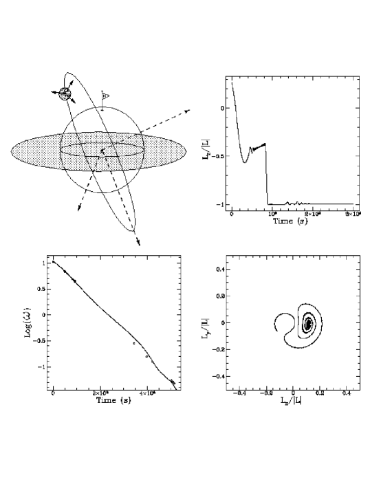
FIG. 3.: The spin dynamics of LAGEOS: Numerical results. We present here results from our numerical simulation of the dynamic evolution of the LAGEOS satellite (here modeled as a slightly oblate spheroid of brass orbiting an earth-like mass idealized as perfectly spherical and endowed with a polar-oriented dipole magnetic field, top left figure). The evolution of the satellite’s angular momentum reveals three unique phases, as demonstrated in the plot of the component of angular momentum orthogonal to the orbital plane (top right). The first phase is characterized by an exponential decrease in spin of the satellite, with negligible nutation and precession. The decay in spin for a $25.55~{}cm$ radius sphere of brass agrees with the data (bottom left). In the spin-orbit resonance phase the angular velocity decays to a value comparable to the orbital angular velocity. The nutation and precession increase, and the angular momentum vector lifts off the orbital plane and settles down orthogonal to the orbital plane (top right). The third phase (asymptotic) is characterized by the tidal locking of the satellite.

VI Results.

We have identified three distinct phases in the spin dynamics of the LAGEOS satellite (Figs. 3-5), which we shall refer to as (1) the Fast Spin Phase, (2) the Spin-Orbit Resonance Phase, and (3) the Asymptotic Phase.

a) Fast Spin Phase. This first phase, from $t=0$ to $t\sim 25~{}yrs$, is characterized by an exponential decrease in the spin rate ($\dot{\psi}$) of the satellite (Fig. 3) from $\dot{\psi}(t=0)=10.7709~{}s^{-1}$ to $\dot{\psi}(t\sim 25~{}yrs)\approx.001~{}s^{-1}$. The body axis of the satellite is aligned with the angular momentum of the satellite in this phase; hence, all other quantities (angular momentum, kinetic energy, etc.) also decrease exponentially. The nutation of the satellite (the angle between the body axis of the satellite and the normal to the orbital plane) undergoes a steady increase from $\theta_{0}=90~{}\deg$ at $t=t_{0}$ to $\theta\sim 126~{}\deg$ over a period of $\sim 6.4~{}yrs$, indicating a nutation angular velocity of $\bar{\omega}_{\theta}\approx 20~{}\deg/yr$. The nutation then settles down to a “pseudo-stable” state at $\theta\approx 115~{}\deg$ over the next $3.2$ years and remains at this value ($\pm 5\%$) until the onset of the spin-orbit resonance at $\sim 25~{}yrs$ (Fig. 6). Finally, within this twenty five year period the satellite precesses in a positive sense by 63 revolutions before unwinding when entering the spin-orbit resonance phase.

b) Spin-Orbit Resonance Phase. The spin dynamics abruptly change at $t\sim 27~{}yrs$. This is precisely when the satellite’s spin, decreased by magnetic damping, approaches the orbital angular velocity

$$\omega_{orbit}=\sqrt{{3.9\times 10^{20}\over(1.227179\times 10^{9})^{3}}}~{}s^{-1}\approx 0.0004593782~{}s^{-1}.$$ (75)

The conductivity of the satelite was chosen to reproduce experimentally observed exponential decay in the spin rate of the satellite,

$$\dot{\psi}(t)=\psi(t_{0})e^{-{(t-t_{0})\over\Delta}},$$ (76)

with ($\Delta\sim 2.96~{}yr$ time constant). Therefore, the spin-orbit resonance should occur at $t_{sp}\sim 30~{}yrs$, which is in agreement with the numerical results. The resonance phase is marked by a movement of the angular momentum vector to a position orthogonal to the orbital plane, and is furthermore characterized by the beginning of satellite wobble (i.e., the point in time when $\xi$ of Eq. (6) becomes nonzero and the body axis becomes misaligned with the instantaneous angular momentum vector). From this point forward it is more illustrative to examine the dynamics of the instantaneous angular velocity and momentum rather than the Euler angles. In addition to the dramatic changes in the spin dynamics, this second phase also gives rise to a reversal in the signs of the precessional velocity ($\omega_{\phi}$) and spin ($\omega_{\psi}$).

c) The Asymptotic Phase. Following the spin-orbit resonance phase, the spin dynamics gradually settled down to an asymptotic regime over the course of $\sim 50~{}yrs$. Not surprisingly, the satellite becomes tidally locked (think of the moon). In particular, the asymptotic value of the total angular velocity is equal to the orbital angular velocity, subject to small fluctuations. We note that in this phase the torques induced from the changing magnetic field due to orbital motion of the satellite will become important, and should no longer be ignored. However, their addition will not significantly change dynamics, as the energies at this point are quite low.

From our numerical runs, a rough estimate of the asymptotic behavior of the satelite model (modulo phase and a finite offset in $\phi$) is given by

$$\theta(t) \simeq 1.57+0.12\cos(4.6\times 10^{-4}t),$$ (77)

$$\phi(t) \simeq -4.59\times 10^{-4}t,$$ (78)

$$\psi(t) \simeq 3.04+0.115\cos(4.6\times 10^{-4}t),$$ (79)

$$\omega_{\theta}(t) \simeq 5.5\times 10^{-5}\cos(4.6\times 10^{-4}t),$$ (80)

$$\omega_{\phi}(t) \simeq -4.59\times 10^{-4}+3.1\times 10^{-3}\cos(1.4\times 10^{-4}t),$$ (81)

$$\omega_{\psi}(t) \simeq 5.3\times 10^{-5}\cos(4.6\times 10^{-4}t).$$ (82)

The asymptotic values of the other relevant parameters (Fig. 4):

$$K.E. \sim 13.42ergs,$$ (83)

$$-{1\over c}(M\dot{B}) \sim 3.2\times 10^{-8}ergs,$$ (84)

$$G.E. \sim -0.45375ergs\ to\ -0.45ergs,$$ (85)

$$E \sim 12.96ergs,$$ (86)

$$L \sim 5.84\times 10^{4}g\,cm^{2}/s,$$ (87)

$$\hat{L}_{x} \sim 0.115,$$ (88)

$$\hat{L}_{y} \sim -0.15\pm 0.05,$$ (89)

$$\hat{L}_{z} \sim -0.9933,$$ (90)

$$\omega \sim 0.0004595s^{-1}$$ (91)

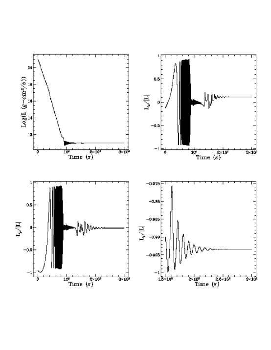
FIG. 4.: The behavior of the angular momentum vector and its components throughout the mission. The evolution of the angular momentum reveals the transition to an asymptotic phase wherein the angular momentum vector is roughly orthogonal to the body axis of the satellite, and is consistent with a precession rate equal to the orbital angular velocity.

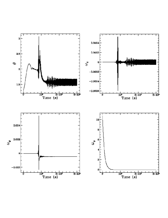
FIG. 5.: Dynamics of the Euler angles. The evolution of the nutation (angle of obliquity, $\theta$) of the model satellite (upper left). In the asymptotic limit the angular velocities of nutation and precession average to zero (upper and lower right, respectively). The precession rate ($\omega_{\phi}$), on the other hand, locks into the orbital velocity (lower left). This last plot demonstrates clearly the dynamics through the spin-orbit resonance phase.

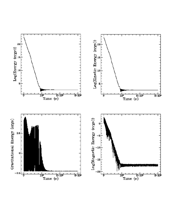
FIG. 6.: Energy. A plot of the logarithm of the total energy of the satellite as a function of time reveals an asymptotic limit of $12.96~{}ergs$ consistent with tidal locking. The linear region early on ($0-9\times 10^{8}~{}s$) reflects the resistive damping phase of the induced eddy currents. Asymptotically, the satellite orients itself so as to minimize the gravitational potential energy (lower left) while the magnetic energy (${1\over c}M\cdot B$) becomes negligible.

VII Conclusions.

Of the five largest sources of error identified in the LAGEOS-3 experiment, the earth and solar-induced surface forces are potentially the most troublesome (Table I). The anisotropic heating of the satellite, and subsequent reradiation, gives a “thermal rocketing” perturbation (referred to as the Rubincam effect or the Yarkowsky thermal drag) which tends to degrade the experiment. To model this effect requires, in part, a detailed knowledge of the behavior of the angular momentum of the satellite. Toward this end we have derived, and solved numerically, a simplified set of Euler equations that evolve the angular momentum vector for a slightly oblate spheroid of brass orbiting an earth-like mass, idealized as being a perfect sphere and having a perfect polar-oriented dipole magnetic field. The Euler equations included both the tidal gravitational torques and the eddy-current torques, as well as the resistive damping torques, as modeled by complex magnetization coefficients. Using this rather simplified model, we have identified three phases of the rotational dynamics – a fast spin phase, a spin-orbit resonance phase, and an asymptotic phase (Fig. 3). We have also identified an error in the previously established model of asymptotic spin dynamics [7]. This error has led to confusion and, in attempts to reconcile observed data with theoretical predictions, has led others to hypothesize erroneous models for the moments of inertia of LAGEOS-1 [14].

Our results have led us to formulate four as yet unresolved questions: (1) Can we obtain the asymptotic solution analytically, and in so doing can we understand the wobbling or slippage of the Euler angles with respect to the relatively stable total instantaneous angular velocity?; (2) Can we understand why the rms fluctuations in the gravitational potential energy cause the asymptotic value of the angular momentum vector to be offset from the orbital plane by $\sim 10~{}deg$?; (3) Can we understand why the nutation angle ($\theta$) drifts initially at a rate of $\sim 20~{}deg/yr$ and reaches a pseudo-stable value of $\sim 115~{}deg$?; and (4) Can we understand the fluctuations in the spin rate ($\dot{\psi}$) over the first $\sim 20~{}yrs$, which do not appear to have been detected experimentally? We are addressing these questions by (1) introducing a more realistic model of the satellite and earth into our calculations [15], and (2) exploring more of phase space by way of Poincare sections. The results presented here provide us with clues that must be pieced together to reveal the physics behind the complex motion we observe.

The current spin dynamics model suggests that we launch LAGEOS-3, with as large a spin $(\dot{\psi})$ as possible, into an obliquity of $\theta\sim 115~{}\deg$; although, due to the qualitative nature of our results, the precise numbers are far from being conclusive.

We are currently working with the Center for Space Research at the University of Texas at Austin to determine the impact this revised model of the spin dynamics of LAGEOS will have on the LAGEOS-3 mission (in particular, how will the Rubincam effect alter the line of nodes of the orbital plane?). In addition, we are working closely with colleagues at the University of Texas and the University of Maryland to reconcile the experimental measurements of the spin dynamics of LAGEOS-1 with our theoretical model [16]. Furthermore, we will propose an optimal experimental measurement schedule in support of the proposed LAGEOS-3 mission.

REFERENCES

- [1] J. M. Bardeen and J. A. Peterson, App. J. Lett. 195, L65 (1975); D. A. MacDonald, K. S. Thorne, R. H. Price and Xiao-He Zhang, Astrophysical Applications of Black Hole Electrodynamics in Black Holes: The Membrane Paradigm, edited by K. S. Thorne, R. H. Price, and D. A. MacDonald (Yale University Press, New Haven, 1986), Ch. 4.
- [2] H. Thirring and J. Lense, Phys. Z. 19, 156 (1918); H. Thirring, ibid 19, 33 (1918), ibid 22, 29 (1921). An English translation is given by B. Mashhoon, F. W. Hehl, and D. S. Theiss, Gen. Relativ. Gravit. 16, 711 (1984).
- [3] C. W. F. Everitt, in Experimental Gravitation, edited by B. Bertotti (Academic, New York, 1973); R. A. VanPatten and C. W. F. Everitt, Phys. Rev. Lett. 36 (1976).
- [4] I. Ciufolini Phys. Rev. Lett. 56, 278 (1986).
- [5] J. Ries, private communication (1993).
- [6] D. P. Rubincam, J. Geophys Research 92, 1278-1294 (1987); ibid 93, 13805 (1988); ibid 95, 4881 (1990); The LAGEOS Along Track Acceleration: A Review, Paper presented at the First William Fairbanks meeting on relativistic gravity experiments in space, Rome, Italy, September 10-14, 1990.
- [7] B. Bertotti B. and L. Iess, J. Geophys. Research 96, 2431 (1991).
- [8] J. P. Vinti, Theory of the Spin of a Conducting Satellite in the Magnetic Field of the Earth, Defense Technical Information Center, BRL-1020 (1957).
- [9] H. Goldstein, Classical Mechanics (Addison-Wesley, Reading, MA, 1981).
- [10] C. Fuchs, Lagrangian formulation of LAGEOS’s spin dynamics, Final Report, 1992 Air Force Summer Research Program, August 1992.
- [11] C. W. Johnson, C. A. Lundquist, and J. L. Zurasky, The LAGEOS satellite, Paper presented at the International Astronautical Federation XXVII Congress, Anaheim, CA, October 10-16, 1976).
- [12] L. D. Landau and E. M. Lifshitz, Electrodynamics of Continuous Media (Pergamon Press, Oxford, 1984).
- [13] W. H. Press, S. A. Teukolsky, W. T. Vetterling, and B. P. Flannery, Numerical Recipes in C (Cambridge University Press, Cambridge, 1992).
- [14] R. Scharroo, K. F. Wakker, B. A. C. Ambrosius, and R. Noomen, J. Geophys. Research 96, 729 (1991).
- [15] R. P. Halverson and H. Cohen, IEEE Trans. Aerosp. Navig. Electron. ANE-11, 118 (1964).
- [16] D. Currie, S. Habib, R. Matzner, and W. A. Miller, (in preparation).