Invariance Properties of Boundary Sets of Open Embeddings of Manifolds and Their Application to the Abstract Boundary

Abstract

The abstract boundary (or a-boundary) of Scott and Szekeres [5] constitutes a “boundary” to any $n$-dimensional, paracompact, connected, Hausdorff, $C^{\infty}$-manifold (without a boundary in the usual sense). In general relativity one deals with a space-time $({\cal M},g)$ (a 4-dimensional manifold ${\cal M}$ with a Lorentzian metric $g$), together with a chosen preferred class of curves in ${\cal M}$. In this case the a-boundary points may represent “singularities” or “points at infinity”. Since the a-boundary itself, however, does not depend on the existence of further structure on the manifold such as a Lorentzian metric or connection, it is possible for it to be used in many contexts.

In this paper we develop some purely topological properties of abstract boundary sets and abstract boundary points (a-boundary points). We prove, amongst other things, that compactness is invariant under boundary set equivalence, and introduce another invariant concept (isolation), which encapsulates the notion that a boundary set is “separated” from other boundary points of the same embedding. It is demonstrated, however, that the properties of connectedness and simple connectedness of boundary sets are not invariant under boundary set equivalence.

We introduce a $T$ neighbourhood property (n$T$NP) of boundary sets, where $T$ is any topological property of a topological space, i.e., a property invariant under all homeomorphisms of the space. It is shown that any such n$T$NP is invariant under boundary set equivalence. The connected neighbourhood property (n$C$NP) and the simply connected neighbourhood property (n$SC$NP) are examined in detail. It is proven, for instance, that any boundary set satisfying the n$C$NP must be connected. We conclude with a consideration of (isolated) boundary sets which are also submanifolds of the enveloping manifold. When the above concepts appear, throughout the paper, they are related to the abstract boundary (i.e., the set of equivalence classes of boundary sets which include a singleton).

1 Introduction

We briefly summarise the construction of the a-boundary as presented in [5], and fix our notation. Only the first part of that paper is needed here, before the introduction of a pseudo-Riemannian metric and the ensuing classification of a-boundary points.

All manifolds will be assumed to be smooth (i.e., $C^{\infty}$), Hausdorff, connected and paracompact manifolds without boundary, unless otherwise stated. We call a $C^{\infty}$ embedding $\phi:{\cal M}\to{\widehat{{\cal M}}}$, where ${\cal M}$, ${\widehat{{\cal M}}}$ are manifolds of the same dimension $n$, an envelopment, and denote this $({\cal M},{\widehat{{\cal M}}},\phi)$ (or sometimes, somewhat loosely, $\phi$). The topological boundary of the image $\phi({\cal M})$ in ${\widehat{{\cal M}}}$, $\partial(\phi({\cal M}))$, is denoted $\partial_{\phi}{\cal M}$ or just $\partial_{\phi}$. A boundary set of an envelopment is a subset $B\subset\partial_{\phi}$. The abstract boundary consists of special equivalence classes of boundary sets, in various envelopments, under a certain equivalence relation. This addresses the difficulty one faces in defining space-time “boundary points” in general relativity, for instance, where the topology of the “boundary point” is certainly not invariant under diffeomorphisms of the space-time (i.e., various envelopments).

The equivalence relation used is defined as follows. Suppose that we are given boundary sets $B,\,B^{\prime}$ of two envelopments $({\cal M},{\widehat{{\cal M}}},\phi)$, $({\cal M},{\widehat{{\cal M}}}^{\prime},\phi^{\prime})$, respectively. We say that $B$ covers $B^{\prime}$, in this paper abbreviated to $B\rhd B^{\prime}$, if for every open neighbourhood ${\cal U}$ of $B$ in ${\widehat{{\cal M}}}$, there is an open neighbourhood ${\cal U}^{\prime}$ of $B^{\prime}$ in ${\widehat{{\cal M}}}^{\prime}$ such that

$$\phi\circ(\phi^{\prime}{)}^{-1}({\cal U}^{\prime}\cap\phi^{\prime}({\cal M}))\subset{\cal U}.$$

This encapsulates the idea that “one cannot approach $B^{\prime}$ from within ${\cal M}$ without also approaching $B$”. In fact, using this notation, we quote a theorem:

Theorem 19 of [5]. $B\rhd B^{\prime}$ if and only if, for any sequence $\{p_{i}\}$ of points of ${\cal M}$ such that the sequence $\{\phi^{\prime}(p_{i})\}$ has a limit point in $B^{\prime}$, the sequence $\{\phi(p_{i})\}$ has a limit point in $B$.

One then says that boundary sets $B$ and $B^{\prime}$ are equivalent, $B\sim B^{\prime}$, if they cover each other: $B\rhd B^{\prime}$ and $B\lhd B^{\prime}$. The equivalence class containing the boundary set $B$ is denoted $[B]$, and is called an abstract boundary set. If $[B]$ contains a singleton boundary set $\{p\}$, then $[B]$ may also be denoted by $[p]$, and is called an abstract boundary point.

The collection of all abstract boundary points constitutes the abstract boundary ${\cal B}({\cal M})$ of ${\cal M}$; that is,

$${\cal B}({\cal M})\mathop{=}\limits^{\hbox{\footnotesize def}}\left\{\>[p]\mathbin{:}p\in\partial_{\phi}{\cal M}\hbox{ for some envelopment }({\cal M},{\widehat{{\cal M}}},\phi)\>\right\}.$$

For further details of this construction, see [5].

We will assume that primed objects belong to an envelopment $({\cal M},{\widehat{{\cal M}}}^{\prime},\phi^{\prime})$ unless otherwise stated, with corresponding unprimed objects belonging to an envelopment $({\cal M},{\widehat{{\cal M}}},\phi)$.

2 Compact boundary sets

We note that any paracompact, connected, Hausdorff, smooth manifold ${\cal M}$ can be given a Riemannian metric $g_{0}$ by using a partition of unity to “smooth out” Riemannian metrics on the domains of local coordinate charts (see, e.g., [2]). Further, any (smooth) Riemannian metric $g_{0}$ on ${\cal M}$ is globally conformal to a (smooth) complete Riemannian metric $g$ [4], i.e., $g=\Omega^{2}g_{0}$ where $\Omega$ is a smooth, positive-valued function on ${\cal M}$. Now $g$ induces a complete [topological] metric $d$, which is the distance function given by $d(p,q)=\inf\{$Riemannian arc lengths of piecewise smooth curves connecting $p$ and $q\}$. We shall use the term “Riemannian metric” for $d$ as well as for $g$, and we will assume them to be complete, unless otherwise stated.

The metric topology of $d$ agrees with the given manifold topology on ${\cal M}$. Since $d$ is complete, the Hopf-Rinow Theorem (see, e.g., [1]) says that every subset $K$ of ${\cal M}$ for which $d$ is bounded (i.e., $\sup\left\{\>d(p,q)\mathbin{:}p,q\in K\>\right\}<\infty$) has compact closure. The ability to connect compactness and boundedness in this way is the reason we implement complete metrics extensively throughout this paper.

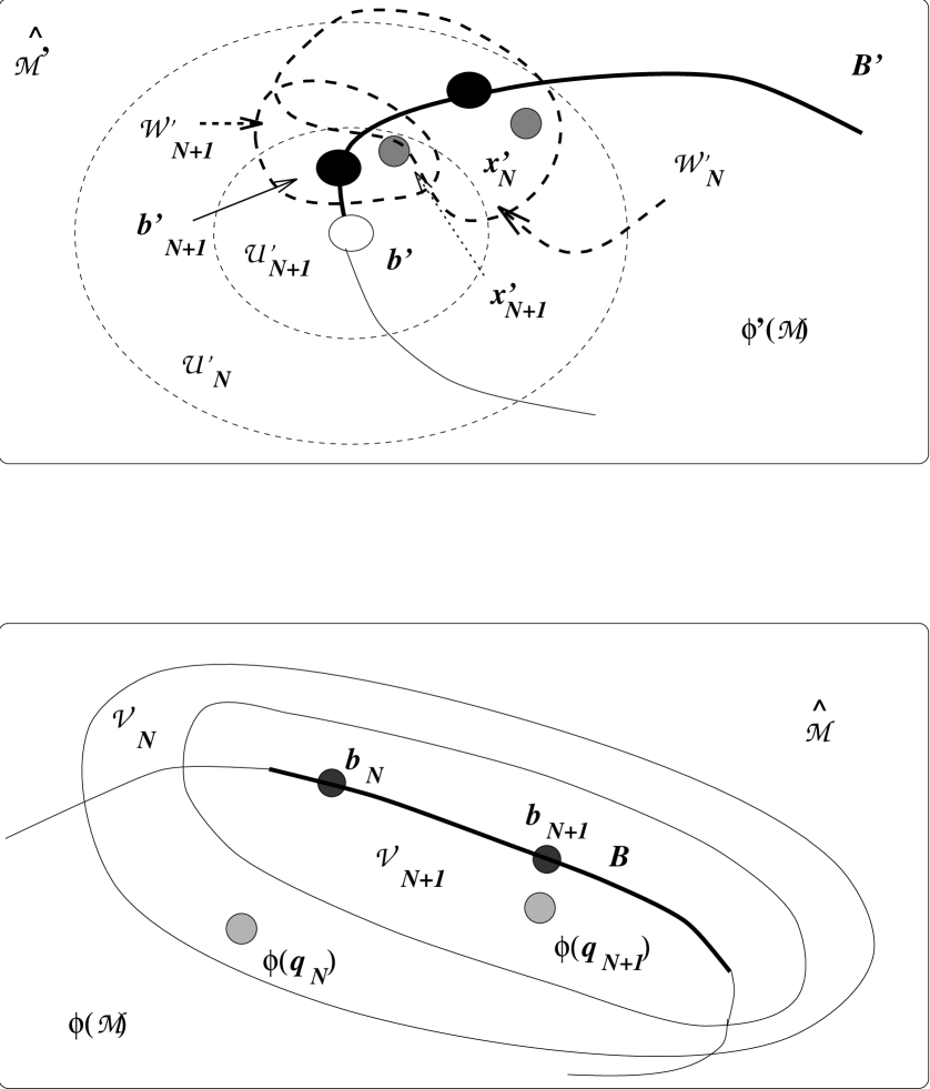
Figure 1: Proof of Lemma 2.1.

The following lemma demonstrates that if a boundary set of a given envelopment is compact, then all boundary sets (of other envelopments) which are equivalent to it must be closed.

Lemma 2.1.

If a boundary set $B\subset\partial_{\phi}$ is compact, then any $B^{\prime}\sim B$ is closed.

Proof 2.2.

(As usual $B\subset\partial_{\phi},B^{\prime}\subset\partial_{\phi^{\prime}}$.)

Let $d,d^{\prime}$ be complete Riemannian metrics on ${\widehat{{\cal M}}},{\widehat{{\cal M}}}^{\prime}$ respectively. Define

$${\cal V}_{N}\mathop{=}\limits^{\hbox{\footnotesize def}}\left\{\>y\in{\widehat{{\cal M}}}\mathbin{:}d(y,b)<1/N\hbox{ for some }b\in B\>\right\},\qquad N\in{\mathbb{N}}.$$

Now suppose that $B^{\prime}\sim B$ and that $b^{\prime}\in\overline{B^{\prime}}\setminus B^{\prime}$. Define

$${\cal U}^{\prime}_{N}\mathop{=}\limits^{\hbox{\footnotesize def}}\left\{\>x^{\prime}\in{\widehat{{\cal M}}}^{\prime}\mathbin{:}d^{\prime}(b^{\prime},x^{\prime})<1/N\>\right\},\qquad N\in{\mathbb{N}}.$$

There exists $b_{N}^{\prime}\in{\cal U}^{\prime}_{N}\cap B^{\prime}$, for each $N$.

Since $B\rhd b_{N}^{\prime}$ [5, Theorem 16], there exists an open neighbourhood ${\cal W}^{\prime}_{N}$ of $b^{\prime}_{N}$ in ${\widehat{{\cal M}}}^{\prime}$ such that

$$\phi\circ(\phi^{\prime}{)}^{-1}({\cal W}^{\prime}_{N}\cap\phi^{\prime}({\cal M}))\subset{\cal V}_{N}.$$

Since $b^{\prime}_{N}$ is in the open set ${\cal U}^{\prime}_{N}\cap{\cal W}^{\prime}_{N}$ and $b_{N}^{\prime}\in\partial_{\phi^{\prime}}$, there clearly exists an $x_{N}^{\prime}\in{\cal U}^{\prime}_{N}\cap{\cal W}^{\prime}_{N}\cap\phi^{\prime}({\cal M})$. See Figure 1.

Let $q_{N}\mathop{=}\limits^{\hbox{\footnotesize def}}(\phi^{\prime}{)}^{-1}(x^{\prime}_{N})$, $\forall\;N\in{\mathbb{N}}$, so that $\{q_{N}\}$ is a sequence of points in ${\cal M}$ such that $\phi^{\prime}(q_{N})=x^{\prime}_{N}\to b^{\prime}$. Since $\phi(q_{N})\in{\cal V}_{N}$, there is a $b_{N}\in B$ such that $d(b_{N},\phi(q_{N}))<1/N$.

Now $\{b_{N}\}$ is an infinite sequence of boundary points in $B$ and so must have a limit point $b^{\ast}$ in $B$ (since $B$ is compact). Choose the first element $b_{N_{1}}$ of the sequence $\{b_{N}\}$ that satisfies $d(b^{\ast},b_{N_{1}})<1$ and set $p_{1}=q_{N_{1}}$. Next choose the first element $b_{N_{2}}$ of the sequence $\{b_{N}\}$ occurring after $b_{N_{1}}$ that satisfies $d(b^{\ast},b_{N_{2}})<1/2$ and set $p_{2}=q_{N_{2}}$. Continue in this manner to form the infinite sequence $\{p_{i}\}$ in ${\cal M}$ where for any $i\in{\mathbb{N}}$, $d(b^{\ast},b_{N_{i}})<1/i$. Since $i\leq N_{i}$, $\forall\;i\in{\mathbb{N}}$,

$$d(b_{N_{i}},\phi(p_{i})) = d(b_{N_{i}},\phi(q_{N_{i}}))$$

$$< 1/N_{i}$$

$$\leq 1/i,$$

and

$$d(b^{\ast},\phi(p_{i})) \leq d(b^{\ast},b_{N_{i}})+d(b_{N_{i}},\phi(p_{i}))$$

$$< 1/i+1/i=2/i.$$

Thus $\phi(p_{i})\to b^{\ast}$.

Since $B^{\prime}\rhd B$, the sequence $\{\phi^{\prime}(p_{i})\}$ must have a limit point in $B^{\prime}$ [5, Theorem 19]. However, $\phi^{\prime}(q_{N})\to b^{\prime}$ and so $\phi^{\prime}(p_{i})\to b^{\prime}\not\in B^{\prime}$, which gives a contradiction.

Thus $\overline{B^{\prime}}=B^{\prime}$.

Note that in the above lemma it is not sufficient to assume that $B$ is merely closed, as opposed to compact. That is, closedness is not invariant under boundary set equivalence, as will be clearly demonstrated by the following example.

Example 2.3.

Let ${\widehat{{\cal M}}}={\mathbb{R}}^{3}$, ${\cal M}=\left\{\>(x,y,z)\in{\mathbb{R}}^{3}\mathbin{:}z<0\>\right\}$, $\phi={}$inclusion, and $B=\partial_{\phi}=\{z=0\}$, a plane (closed, but non-compact).

Now compactify ${\cal M}$ to an open box $\{|x|,|y|,|z|<1,z<0\}$ in ${\mathbb{R}}^{3}$. So ${\widehat{{\cal M}}}^{\prime}={\mathbb{R}}^{3}$, $\phi^{\prime}({\cal M})=\{|x|,|y|,|z|<1,z<0\}$, and $B\sim B^{\prime}$ where $B^{\prime}$ is the “top face” $\{z=0,|x|,|y|<1\}$ of $\phi^{\prime}({\cal M})$, which does not include the perimeter $\{z=0,\,|x|,|y|\leq 1$ and either $|x|$ or $|y|=1\}$. $B^{\prime}$ is most certainly not closed.

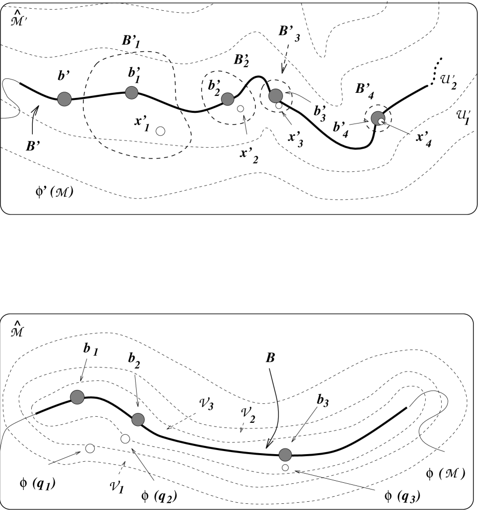
Figure 2: Proof of Theorem 2.4.

Theorem 2.4 which follows establishes that compactness is invariant under boundary set equivalence. So if a boundary set of a given envelopment is compact, then all boundary sets equivalent to it must be compact. This, of course, implies that an abstract boundary set $[B]$ may be labelled “compact” if and only if $B$ is compact.

Theorem 2.4.

If a boundary set $B\subset\partial_{\phi}$ is compact, then any $B^{\prime}\sim B$ is compact.

Proof 2.5.

Assume that $B^{\prime}$ is not compact and let $d,d^{\prime}$ be complete Riemannian metrics on ${\widehat{{\cal M}}},{\widehat{{\cal M}}}^{\prime}$ respectively. Since $B^{\prime}$ is closed by Lemma 2.1, $B^{\prime}$ cannot be bounded with respect to $d^{\prime}$ (see the remark at the beginning of this section).

Fix $b^{\prime}\in B^{\prime}$, and choose $b^{\prime}_{1}\in B^{\prime}$ so that $d^{\prime}(b^{\prime},b^{\prime}_{1})>1$. Next choose $b^{\prime}_{2}\in B^{\prime}$ with $d^{\prime}(b^{\prime},b^{\prime}_{2})>2$ and $d^{\prime}(b^{\prime}_{1},b^{\prime}_{2})>1$. Continue in this manner to form an infinite sequence $\{b^{\prime}_{n}\}$ of boundary points in $B^{\prime}$ such that $d^{\prime}(b^{\prime}_{m},b^{\prime}_{n})>1$, $\forall\>m,n\in{\mathbb{N}}$ ($m\neq n$), and $d^{\prime}(b^{\prime},b^{\prime}_{n})>n$, $\forall\>n\in{\mathbb{N}}$ (this is possible due to the unbounded nature of $B^{\prime}$). Thus $d^{\prime}(b^{\prime},b^{\prime}_{n})\to\infty$ as $n\to\infty$. Now let

$$B_{n}^{\prime}\mathop{=}\limits^{\hbox{\footnotesize def}}\left\{\>x^{\prime}\in{\widehat{{\cal M}}}^{\prime}\mathbin{:}d^{\prime}(b^{\prime}_{n},x^{\prime})<1/2n\>\right\},\qquad n=1,2,\ldots.$$

Each $B^{\prime}_{n}$ is open, and clearly $B_{m}^{\prime}\cap B_{n}^{\prime}=\emptyset$ for all $m\neq n$. Now let

$${\cal V}_{n}\mathop{=}\limits^{\hbox{\footnotesize def}}\left\{\>y\in{\widehat{{\cal M}}}\mathbin{:}d(b,y)<1/2n\hbox{ for some }b\in B\>\right\},\qquad n=1,2,\ldots,$$

again open sets (this time in ${\widehat{{\cal M}}}$).

Since $B\rhd B^{\prime}$, for each ${\cal V}_{n}$ there is an open set ${\cal U}^{\prime}_{n}$ of ${\widehat{{\cal M}}}^{\prime}$ containing $B^{\prime}$ such that

$$\phi\circ(\phi^{\prime}{)}^{-1}({\cal U}^{\prime}_{n}\cap\phi^{\prime}({\cal M}))\subset{\cal V}_{n}.$$

Since $b^{\prime}_{n}\in{\cal U}^{\prime}_{n}\cap B^{\prime}_{n}$ which is open, and $b_{n}^{\prime}\in\partial_{\phi^{\prime}}$, there exists an $x^{\prime}_{n}\in{\cal U}^{\prime}_{n}\cap B^{\prime}_{n}\cap\phi^{\prime}({\cal M})$. Let $q_{n}\mathop{=}\limits^{\hbox{\footnotesize def}}(\phi^{\prime}{)}^{-1}(x^{\prime}_{n})$, $\forall\;n\in{\mathbb{N}}$. Since $\phi(q_{n})\in{\cal V}_{n}$, there exists a $b_{n}\in B$ such that $d(b_{n},\phi(q_{n}))<1/2n$. See Figure 2.

Exactly as in the proof of Lemma 2.1, $\{b_{n}\}$ is an infinite sequence of boundary points in $B$ and so must have a limit point $b^{\ast}$ in $B$ (since $B$ is compact). Choose the first element $b_{n_{1}}$ of the sequence $\{b_{n}\}$ that satisfies $d(b^{\ast},b_{n_{1}})<1/2$, and set $p_{1}=q_{n_{1}}$. Next choose the first element $b_{n_{2}}$ of the sequence $\{b_{n}\}$ occurring after $b_{n_{1}}$ and satisfying $d(b^{\ast},b_{n_{2}})<1/4$, and set $p_{2}=q_{n_{2}}$. Continue in this manner to form the infinite sequence $\{p_{i}\}$ in ${\cal M}$ where for any $i\in{\mathbb{N}}$, $d(b^{\ast},b_{n_{i}})<1/2i$. Since $i\leq n_{i}$, $\forall\;i\in{\mathbb{N}}$,

$$d(b_{n_{i}},\phi(p_{i})) = d(b_{n_{i}},\phi(q_{n_{i}}))$$

$$< 1/2n_{i}$$

$$\leq 1/2i,$$

and

$$d(b^{\ast},\phi(p_{i})) \leq d(b^{\ast},b_{n_{i}})+d(b_{n_{i}},\phi(p_{i}))$$

$$< 1/2i+1/2i=1/i.$$

Thus $\phi(p_{i})\to b^{\ast}$.

Since $B^{\prime}\rhd B$, the sequence $\{\phi^{\prime}(p_{i})\}$ must have a limit point $\tilde{b}^{\prime}$ in $B^{\prime}$ [5, Theorem 19], and $d^{\prime}(b^{\prime},\tilde{b}^{\prime})=X\in{\mathbb{R}},\,X\geq 0$. Also

$$d^{\prime}(b^{\prime},\phi^{\prime}(p_{i})) = d^{\prime}(b^{\prime},\phi^{\prime}(q_{n_{i}}))$$

$$= d^{\prime}(b^{\prime},x^{\prime}_{n_{i}})$$

$$\geq d^{\prime}(b^{\prime},b^{\prime}_{n_{i}})-d^{\prime}(b^{\prime}_{n_{i}},x^{\prime}_{n_{i}})$$

$$> d^{\prime}(b^{\prime},b^{\prime}_{n_{i}})-1/2n_{i}.$$

Thus $d^{\prime}(b^{\prime},\phi^{\prime}(p_{i}))\to\infty$ as $i\to\infty$. However,

$$d^{\prime}(\tilde{b}^{\prime},\phi^{\prime}(p_{i})) \geq d^{\prime}(b^{\prime},\phi^{\prime}(p_{i}))-d^{\prime}(b^{\prime},\tilde{b}^{\prime})$$

$$= d^{\prime}(b^{\prime},\phi^{\prime}(p_{i}))-X.$$

It follows that $d^{\prime}(\tilde{b}^{\prime},\phi^{\prime}(p_{i}))\to\infty$ as $i\to\infty$. This contradicts the fact that $\tilde{b}^{\prime}$ is a limit point of the sequence $\{\phi^{\prime}(p_{i})\}$.

Thus $B^{\prime}$ must be compact.

Corollary 2.6.

All boundary sets equivalent to a boundary point are compact.

In particular, this means that the label “compact” may be transferred to every abstract boundary point $[p]$ contained in the abstract boundary ${\cal B}({\cal M})$ of ${\cal M}$, since for any boundary set $B$ such that $[B]=[p]$, $B$ must be compact. One might ask whether any compact abstract boundary set $[B]$ exists such that $[B]\not\in{\cal B}({\cal M})$. The answer to this question is yes: see Examples 4.19 and 5.1.

3 Isolated boundary sets

3.1 Definition and properties

It is often of interest to consider boundary sets which are, in some sense, not close to any other boundary points of the given envelopment. This notion is encapsulated by the following definition of an isolated boundary set.

Definition 3.1.

A compact boundary set $B$ is said to be isolated if there is an open neighbourhood (in ${\widehat{{\cal M}}}$) ${\cal U}$ of $B$ such that

$${\cal U}\cap\partial_{\phi}=B.$$

Note that compactness is assumed here. The following examples show why closedness and boundedness are both necessary assumptions of the above definition.

• What is wrong with $B$ open?

  Consider $({\cal M},{\widehat{{\cal M}}},\phi)$ to be the same as in Example 2.3. Let ${\cal U}$ be an open ball cutting the $z=0$ plane and let $B={\cal U}\cap\partial_{\phi}$, a boundary set which we obviously would not wish to call “isolated”—it is in no sense “separated” from the rest of the boundary (c.f. Lemma 3.2).

• What is wrong with $B$ unbounded?

  Again we consider Example 2.3. We note that the boundary set $B$ (as given in Example 2.3) would be isolated if compactness were not required, but $B\sim B^{\prime}$ and $B^{\prime}$ is again of the type given in Example (i) above which we would not want to call “isolated”.

The sense in which Examples (i) and (ii) are undesirable is expressed precisely in the following useful lemma. First, we recall some topology.

A subset $Y$ of a topological space $X$ is connected iff it cannot be expressed as the disjoint union of two non-empty sets which are open in the relative topology of $Y$. Equivalently, $Y$ is connected iff it contains no proper, non-empty subsets which are both open and closed in the relative topology of $Y$. A subset which is not connected is disconnected.

A component of a topological space is a maximal connected subset, i.e., a connected subset properly contained in no other. A topological space is the disjoint union of its components.

Note that we do not require that components be open because then, for instance, the closed unit interval $[0,1]$ in

$$[0,1]\cup\Bigl{(}\bigcup_{n\in{\mathbb{N}}}\{-1/n\}\Bigr{)}$$

would lie in no “component”! Components are closed, however, for a component together with any of its limit points which it did not contain would be connected and properly contain the original. Any non-empty subset which is both open and closed is a union of components of the topological space.

It turns out to be useful to use the concept of local finiteness of a collection of subsets of the boundary: we say that the collection $\{{\cal U}_{\alpha}\}$, ${\cal U}_{\alpha}\subset X$, is locally finite if each $p\in X$ has an open neighbourhood ${\cal W}$ which intersects only finitely many of the ${\cal U}_{\alpha}$. A moment’s thought shows that the concept of local finiteness of a collection $\{{\cal U}_{\alpha}\},\,{\cal U}_{\alpha}\subset Y\subset X$, is independent of whether one takes the open neighbourhoods ${\cal W}$ to be sets of the $X$-topology or the relative $Y$-topology. In the following we will choose the former as this fits more with one’s intuitive idea of a “neighbourhood” of a boundary component.

Lemma 3.2.

1. ()en:comp lem 1 An isolated boundary set $B$ is a union of components of $\partial_{\phi}$ (in the latter’s relative topology).

2. ()en:comp lem 2 The boundary $\partial_{\phi}$ consists of a locally finite collection of boundary components if and only if one can find disjoint ${\widehat{{\cal M}}}$-open neighbourhoods of each component. Any boundary component which is compact is thereby an isolated boundary set.

3. ()en:comp lem 3 If $B=\bigcup B_{i}$ is an isolated boundary set, each $B_{i}$ is a boundary component, and the $B_{i}$ are separated by ${\widehat{{\cal M}}}$-open neighbourhoods ${\cal U}_{i}$, all of which are disjoint, then $B$ is a union of a finite number of boundary components.

Remarks. Even though an isolated boundary set is necessarily compact, it may not be expressible as a finite union of components of $\partial_{\phi}$. Consider the boundary set $B=\partial_{\phi}$ defined by

$$\left\{\begin{array}[]{l}\partial_{\phi}=X\times\{0\},\hbox{ where }X=[0,1]\cup\Bigl{(}\bigcup_{n\in{\mathbb{N}}}\{-1/n\}\Bigr{)}\\ \lx@intercol\hfil{\widehat{{\cal M}}}={\mathbb{R}}^{2},\ \phi({\cal M})={\widehat{{\cal M}}}\setminus\partial_{\phi}\lx@intercol.\end{array}\right.$$ (1)

Then $B$ is isolated but consists of an infinite number of boundary components.

Furthermore, a union $B$ of compact components of the boundary $\partial_{\phi}$ (even if these are finite in number) may not be isolated (although LABEL:en:comp_lem_2 shows that local finiteness of the collection of components of $\partial_{\phi}$ is a sufficient condition for $B$ to be isolated, if it is compact). Every open neighbourhood of the compact component $[0,1]\times\{0\}$ of $\partial_{\phi}$ in (1) above has non-empty intersection with $\partial_{\phi}\setminus([0,1]\times\{0\})$, and so is not isolated.

Finally, we note that “locally finite” may, of course, be replaced by “finite” in the statement of LABEL:en:comp_lem_2 above.

Proof 3.3 (of Lemma 3.2).

To show LABEL:en:comp_lem_1, note that $B$ is compact, so $B$ is closed in ${\widehat{{\cal M}}}$ and thus in $\partial_{\phi}$. Since $B$ is isolated one sees from the definition that it is also open in $\partial_{\phi}$. It follows that it must be a union of components of $\partial_{\phi}$.

We next show the “only if” clause of LABEL:en:comp_lem_2. Let $\{B_{A}\}_{A\in{\cal A}}$ represent the locally finite collection of boundary components. Consider any member of this collection, $B_{A}$. Since $B_{A}$ is a boundary component, it is a closed subset of both $\partial_{\phi}$ and ${\widehat{{\cal M}}}$. Now define

$$X_{A}\mathop{=}\limits^{\hbox{\footnotesize def}}\bigcup_{\stackrel{{\scriptstyle\scriptstyle C\in{\cal A}}}{{C\neq A}}}B_{C}.$$

Suppose that $p\in\overline{X_{A}}\setminus X_{A}$, which implies that $p\in B_{A}$. Since $p\in\overline{X_{A}}$, there is a sequence $\{p_{i}\}$ of points of $X_{A}$ such that $p_{i}\to p$. Now because the collection of boundary components is locally finite, there is an open neighbourhood ${\cal W}$ of $p$ such that ${\cal W}$ intersects only finitely many boundary components: let these (distinct) components be $B_{A}$, $B_{C_{1}},\ldots,B_{C_{m}}$. It follows that there is a subsequence of the $\{p_{i}\}$ lying in one of the $B_{C_{j}}$, whence $p\in\overline{B_{C_{j}}}$. Since $B_{C_{j}}$ is closed, $p\in{B_{C_{j}}}$ and so $p\in X_{A}$, which yields a contradiction. Thus $X_{A}$ is closed, and $X_{A}$ and $B_{A}$ are disjoint closed sets.

Now let $d$ be a Riemannian metric on ${\widehat{{\cal M}}}$. For $p\in B_{A}$, define

$$\mu_{A,p}\mathop{=}\limits^{\hbox{\footnotesize def}}\inf\left\{\>d(p,x)\mathbin{:}x\in X_{A}\>\right\}.$$

Clearly $\mu_{A,p}\geq 0$; assume that $\mu_{A,p}=0$. This means that there is an infinite sequence $\{x_{i}\}$ of points in $X_{A}$ such that $d(p,x_{i})\to 0$ as $i\to\infty$. That is, $x_{i}\to p$ as $i\to\infty$ which implies that $p\in\overline{X_{A}}=X_{A}$. This is a contradiction since $B_{A}$ and $X_{A}$ are disjoint, and thus $\mu_{A,p}>0$.

Now define $\epsilon_{A,p}\mathop{=}\limits^{\hbox{\footnotesize def}}\mu_{A,p}/10$, ${\cal V}_{A,p}\mathop{=}\limits^{\hbox{\footnotesize def}}\left\{\>q\in{\widehat{{\cal M}}}\mathbin{:}d(p,q)<\epsilon_{A,p}\>\right\}$ and

$${\cal U}_{A}\mathop{=}\limits^{\hbox{\footnotesize def}}\bigcup_{p\in B_{A}}{\cal V}_{A,p}.$$

Clearly, ${\cal U}_{A}$ is an open neighbourhood of $B_{A}$.

Consider the collection of open neighbourhoods $\{{\cal U}_{A}\}_{A\in{\cal A}}$. Suppose that $r\in{\cal U}_{C}\cap{\cal U}_{D}$ ($C\neq D$). This implies that $r\in{\cal V}_{C,p}$ for some $p\in B_{C}$ and $r\in{\cal V}_{D,q}$ for some $q\in B_{D}$. Without loss of generality assume that $\epsilon_{C,p}\geq\epsilon_{D,q}$, and then

$$d(p,q) \leq d(p,r)+d(q,r)$$

$$< \epsilon_{C,p}+\epsilon_{D,q}$$

$$\leq 2\epsilon_{C,p}$$

$$= \mu_{C,p}/5.$$

This contradicts that $\mu_{C,p}$ is the greatest lower bound of $\left\{\>d(p,x)\mathbin{:}x\in X_{C}\>\right\}$. Thus $\{{\cal U}_{A}\}_{A\in{{\cal A}}}$ is a collection of disjoint ${\widehat{{\cal M}}}$-open neighbourhoods of the boundary components $\{B_{A}\}_{A\in{{\cal A}}}$. Clearly any boundary component $B_{A}$ which is compact must be an isolated boundary set since ${\cal U}_{A}\cap\partial_{\phi}=B_{A}$.

To show the “if” part of LABEL:en:comp_lem_2: let $p\in\partial_{\phi}$. Now $p$ lies in a particular boundary component $B_{A}$. Thus ${\cal U}_{A}$ is an open neighbourhood of $p$ in ${\widehat{{\cal M}}}$ and ${\cal U}_{A}\cap\partial_{\phi}$ is open in the relative topology of $\partial_{\phi}$. Also ${\cal U}_{A}\cap\partial_{\phi}=B_{A}$, demonstrating that $\{B_{A}\}_{A\in{\cal A}}$ is indeed a locally finite collection of boundary components.

Finally, LABEL:en:comp_lem_3 is immediate. The disjoint ${\widehat{{\cal M}}}$-open neighbourhoods ${\cal U}_{i}$ of the boundary components $B_{i}$ form an open cover $\{{\cal U}_{i}\}$ of $B$. Since $B$ is an isolated boundary set, it is compact. The open cover $\{{\cal U}_{i}\}$ must therefore admit a finite subcover, implying that $B$ is a union of a finite number of boundary components.

3.2 Invariance

The utility of the concept of an isolated boundary set is seen through the following theorem, which establishes that the property of being isolated is invariant under boundary set equivalence.

Theorem 3.4.

If $B\subset\partial_{\phi}$ is an isolated boundary set, then any $B^{\prime}\sim B$ is also an isolated boundary set.

Proof 3.5.

$B^{\prime}$ is compact by Theorem 2.4. Assume that it is not isolated.

Since $B$ is isolated, there is an open neighbourhood (in ${\widehat{{\cal M}}}$) ${\cal U}$ of $B$ such that ${\cal U}\cap\partial_{\phi}=B$. Now let $d$ be a complete Riemannian metric on ${\widehat{{\cal M}}}$. For each $b\in B$, there is a real $\alpha_{b}>0$ such that $\tilde{B}_{b}\subset{\cal U}$, where

$$\tilde{B}_{b}\mathop{=}\limits^{\hbox{\footnotesize def}}\left\{\>x\in{\widehat{{\cal M}}}\mathbin{:}d(b,x)<\alpha_{b}\>\right\}.$$

Let

$$B_{b}\mathop{=}\limits^{\hbox{\footnotesize def}}\left\{\>x\in{\widehat{{\cal M}}}\mathbin{:}d(b,x)<\alpha_{b}/2\>\right\}.$$

So ${\cal U}^{\ast}=\bigcup_{b\in B}B_{b}$ is an open neighbourhood of $B$ in ${\widehat{{\cal M}}}$.

Now since $B$ is compact, there is a finite subcover $\{B_{b_{1}},\ldots,B_{b_{m}}\}$ of the collection $\left\{\>B_{b}\mathbin{:}b\in B\>\right\}$. Of course $A\mathop{=}\limits^{\hbox{\footnotesize def}}\bigcup_{i=1}^{m}B_{b_{i}}$ is an open neighbourhood of $B$ in ${\widehat{{\cal M}}}$. Further, $\bar{A}=\bigcup_{i=1}^{m}\bar{B}_{b_{i}}$ is compact.

Let $x\in\bar{A}\setminus B$: say $x\in\bar{B}_{b_{i}}$. Then $x\in\tilde{B}_{b_{i}}$, so $x\in{\cal U}$. Since $x\not\in B$ and ${\cal U}\cap\partial_{\phi}=B$, $x\not\in\partial_{\phi}$, and it follows that $\bar{A}\cap\partial_{\phi}=B$.

Since $B\rhd B^{\prime}$, there is an open neighbourhood ${\cal V}^{\prime}$ of $B^{\prime}$ in ${\widehat{{\cal M}}}^{\prime}$ such that

$$\phi\circ(\phi^{\prime}{)}^{-1}({\cal V}^{\prime}\cap\phi^{\prime}({\cal M}))\subset A.$$

Now $B^{\prime}$ is not isolated so there is a boundary point $\vbox{\halign{\hfil#\hfil\cr$\smash{\scriptscriptstyle\circ}$\crcr\kern 1.0pt\nointerlineskip\cr$b$\crcr}}^{\prime}\in\partial_{\phi^{\prime}}\setminus B^{\prime}$ which lies in ${\cal V}^{\prime}$. Let $\{p_{i}\}$ be a sequence of points in ${\cal M}$ with $\phi^{\prime}(p_{i})\to\vbox{\halign{\hfil#\hfil\cr$\smash{\scriptscriptstyle\circ}$\crcr\kern 1.0pt\nointerlineskip\cr$b$\crcr}}^{\prime}$. There exists an $N\in{\mathbb{N}}$ such that $\phi^{\prime}(p_{i})\in{\cal V}^{\prime}$ for all $i\geq N$, whence $\phi(p_{i})\in A\subset\bar{A}$ ($\forall\;i\geq N$). Since $\bar{A}$ is compact, the sequence $\{\phi(p_{i})\}$ must have a limit point $y\in\bar{A}$. One can show in a straightforward manner that $y\not\in\phi({\cal M})$ and that $y\not\in{\widehat{{\cal M}}}\setminus\overline{\phi({\cal M})}$. That is, $y\in\partial_{\phi}$, so $y\in B$. Now since $B^{\prime}\rhd B$, the sequence $\{\phi^{\prime}(p_{i})\}$ must have a limit point in $B^{\prime}$ [5, Theorem 19], but $\phi^{\prime}(p_{i})\to\vbox{\halign{\hfil#\hfil\cr$\smash{\scriptscriptstyle\circ}$\crcr\kern 1.0pt\nointerlineskip\cr$b$\crcr}}^{\prime}\not\in B^{\prime}$, a contradiction.

Thus $B^{\prime}$ is an isolated boundary set.

4 Connected boundary sets

Unlike compactness and isolation, connectedness of boundary sets is not invariant under boundary set equivalence. Examples of this are easy to construct, in any dimension. We proceed to do so next even for isolated boundary sets.

Example 4.1.

This example shows that for any dimension $n\geq 2$ one can find connected, isolated boundary sets equivalent to boundary sets with any number $g$ of connected components (where $g$ is a positive integer).

First consider the $n=2$ case. Let ${\widehat{{\cal M}}}$ be a compact, connected surface of genus $g$, where $g$ is an integer greater than 0 (so ${\widehat{{\cal M}}}$ is the surface of a sphere with $g$ “handles”, or rather $g$ “holes”—see Figure 3 where the case $g=4$ is depicted; the holes should be arranged in a ring as shown in the Figure). The case $g=2$ is depicted in Figure 4.

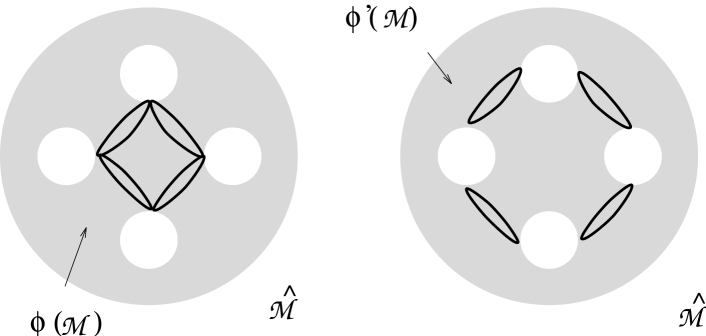
Figure 3: A schematic representation of the compact, connected surface of genus $4$ as discussed in Example 4.1. The shaded areas represent one side of the surface, and the black lines represent the boundary sets in question.

Figure 4: The $g=2$ case of Example 4.1.

Let $B$ consist of $g$ embedded circles (see the Figures). If $g>2$, each circle is to intersect precisely two neighbours, at one point each: each circle “clothes an arm” of the multi-torus. If $g=2$, there is only one neighbouring circle, but there are two intersection points. In the degenerate $g=1$ case there are, of course, no neighbours.

Let ${\cal M}$ be the component of ${\widehat{{\cal M}}}\setminus B$ which does not include those portions of the surface in the centre of ${\widehat{{\cal M}}}$—see the Figures. Let $\phi$ be the inclusion. Then $B=\partial_{\phi}$ is a connected, compact and indeed isolated boundary set.

Let ${\widehat{{\cal M}}}^{\prime}={\widehat{{\cal M}}}$ and $\phi^{\prime}$ be a re-embedding of $\phi({\cal M})$ onto $\phi^{\prime}({\cal M})$, where each “sleeve” of $\phi({\cal M})$, terminating in a circle of $B$, retracts away from the centre of ${\widehat{{\cal M}}}^{\prime}$. Then $B^{\prime}=\partial_{\phi^{\prime}}$ has $g$ components, and clearly we have $B\sim B^{\prime}$.

For $n>2$, consider (with the same notation as above) the envelopments $({\cal M}\times X_{0},{\widehat{{\cal M}}}\times X_{0},\psi\mathop{=}\limits^{\hbox{\footnotesize def}}\phi\times{}$identity$)$ and $({\cal M}\times X_{0},{\widehat{{\cal M}}}^{\prime}\times X_{0},\psi^{\prime}\mathop{=}\limits^{\hbox{\footnotesize def}}\phi^{\prime}\times{}$identity$)$, where $X_{0}$ is any connected, compact manifold. Since $\partial_{\psi}=\partial(\phi({\cal M})\times X_{0})$ is just $\partial_{\phi}\times X_{0}$ (as $X_{0}$ has no boundary, of course), and a product of connected, compact sets is connected and compact, $\partial_{\psi}$ is a connected, isolated boundary set. Similarly, $\partial_{\psi^{\prime}}$ is an isolated boundary set, but consists of $g$ connected components. Now since $\partial_{\psi}\sim\partial_{\psi^{\prime}}$, we have the desired example of a connected, isolated boundary set equivalent to an isolated boundary set with any number of connected components, for any dimension $n\geq 2$.

4.1 The connected neighbourhood property

Example 4.1 demonstrates that connectedness does not “pass to” arbitrary equivalence classes of boundary sets. If, however, a boundary set $B$ of an envelopment $({\cal M},{\widehat{{\cal M}}},\phi)$ satisfies a certain very easily visualised property (the connected neighbourhood property), then one can show that all equivalent boundary sets satisfy this same property. Furthermore, all these equivalent boundary sets must themselves be connected (see Theorem 4.5).

It so happens that this property can very easily be generalised and yet remain invariant under boundary set equivalence (see Theorem 4.9). Below, we define the “connected neighbourhood property” of boundary sets to be a special case of the “$T$ neighbourhood property” of boundary sets, where $T$ is a given topological property.

Definition 4.2.

A topological property $T=T(X)$ of a topological space $X$ is a property of $X$ such that all topological spaces $Y$ which are homeomorphic to $X$ have the same property: i.e., $T(X)\,\Longrightarrow\,T(Y)$ for all $Y$ homeomorphic to $X$.

Definition 4.3.

Let $B$ be a boundary set of an envelopment $({\cal M},{\widehat{{\cal M}}},\phi)$. An open neighbourhood ${\cal U}$ (in ${\widehat{{\cal M}}}$) of $B$ shall be called $T$-nice if its intersection with $\phi({\cal M})$ satisfies $T$ (in the relative topology of ${\cal U}\cap\phi({\cal M})$); i.e., if $T({\cal U}\cap\phi({\cal M}))$ is true.

Definition 4.4.

Using the notation of the previous definition, we will say that $B$ satisfies the $T$ neighbourhood property if all open neighbourhoods ${\cal U}$ of $B$ in ${\widehat{{\cal M}}}$ contain a $T$-nice, open neighbourhood ${\cal V}$ of $B$ (in ${\widehat{{\cal M}}}$). In the following, for the sake of brevity, we will abbreviate “$T$ neighbourhood property” to “n$T$NP”.

In this section we will concentrate on the case

$$T(X)={}\hbox{``$X$ is connected''}{}\mathop{=}\limits^{\hbox{\footnotesize def}}C(X).$$

Thus we have defined the “connected neighbourhood property”, which, in keeping with the abbreviation “n$T$NP”, we shall denote by “n$C$NP”.

We now prove that a boundary set $B$ satisfying the n$C$NP is always connected.

Theorem 4.5.

Let $B$ be a boundary set of an envelopment $({\cal M},{\widehat{{\cal M}}},\phi)$. If $B$ satisfies the n$C$NP, then $B$ is connected.

Proof 4.6.

Suppose that $B$ is disconnected. Then there exist non-empty, open sets ${\cal U}$ and ${\cal V}$ of ${\widehat{{\cal M}}}$ such that

• ${\cal U}\cup{\cal V}$ is an open neighbourhood of $B$,

• ${\cal U}\cap B\neq\emptyset$ and ${\cal V}\cap B\neq\emptyset$, and

• $X\mathop{=}\limits^{\hbox{\footnotesize def}}{\cal U}\cap B$ and $Y\mathop{=}\limits^{\hbox{\footnotesize def}}{\cal V}\cap B$ are disjoint.

That is, $X$ and $Y$ are disjoint, non-empty open sets of the relative topology on $B$, with $X\cup Y=B$.

Let $d$ be a Riemannian metric on ${\widehat{{\cal M}}}$. For any $x\in X$, $y\in Y$, define

$$\rho(x)\mathop{=}\limits^{\hbox{\footnotesize def}}\inf\left\{\>d(x,y)\mathbin{:}y\in Y\>\right\},\qquad\rho(y)\mathop{=}\limits^{\hbox{\footnotesize def}}\inf\left\{\>d(y,x)\mathbin{:}x\in X\>\right\}.$$

Clearly these functions take values in the non-negative reals. We claim that they cannot vanish at any point. Assume that this is not true: without loss of generality, say that $\rho(x)=0$ for some $x\in X$. This implies that there is a sequence $\{y_{m}\}$ of points in $Y$ for which $d(x,y_{m})\mathop{\stackrel{{\scriptstyle m\to\infty}}{{\longrightarrow}}}0$. Since ${\cal U}$ is open, there is some $\mu_{x}>0$ such that $B_{d}(x,\mu_{x})\subset{\cal U}$. This means that $B_{d}(x,\mu_{x})\cap B\subset X$. (Similarly, we define $\mu_{y}$ for $y\in Y$ to be some positive number for which $B_{d}(y,\mu_{y})\subset{\cal V}$, so that $B_{d}(y,\mu_{y})\cap B\subset Y$). It follows, then, that $y_{m}\in X$ eventually, contradicting the disjointness of $X$ and $Y$. Thus $\rho(x),\rho(y)>0$, $\forall\>x\in X,y\in Y$.

For any $x\in X$, $y\in Y$, define

$$\epsilon_{x}\mathop{=}\limits^{\hbox{\footnotesize def}}\min\{\rho(x)/10,\mu_{x}\},\qquad\epsilon_{y}\mathop{=}\limits^{\hbox{\footnotesize def}}\min\{\rho(y)/10,\mu_{y}\}.$$

Clearly $B_{d}(x,\epsilon_{x})\subset{\cal U}$ and $B_{d}(y,\epsilon_{y})\subset{\cal V}$. Let

$$\tilde{\cal U}=\bigcup_{x\in X}B_{d}(x,\epsilon_{x})\qquad\hbox{and}\qquad\tilde{\cal V}=\bigcup_{y\in Y}B_{d}(y,\epsilon_{y}).$$

Assume that $p\in\tilde{\cal U}\cap\tilde{\cal V}$, so $p\in B_{d}(x,\epsilon_{x})$ for some $x\in X$ and $p\in B_{d}(y,\epsilon_{y})$ for some $y\in Y$. Now

$$d(x,y) \leq d(x,p)+d(p,y)$$

$$< 2\max\{\epsilon_{x},\epsilon_{y}\}.$$

Without loss of generality, let us say that $\epsilon_{x}\geq\epsilon_{y}$. Then $d(x,y)<2\epsilon_{x}\leq\rho(x)/5$. This is a contradiction, so that $\tilde{\cal U}$ and $\tilde{\cal V}$ must be disjoint.

Now $\tilde{\cal U}\cup\tilde{\cal V}$ is an open neighbourhood of $B$ in ${\widehat{{\cal M}}}$, and $\tilde{\cal U}\cap B$ and $\tilde{\cal V}\cap B$ are non-empty and disjoint. Since $B$ satisfies the n$C$NP, there exists an open neighbourhood ${\cal W}$ of $B$ with ${\cal W}\subset\tilde{\cal U}\cup\tilde{\cal V}$, for which ${\cal W}\cap\phi({\cal M})$ is connected. Now ${\cal W}\cap\tilde{\cal V}\neq\emptyset$, for were the intersection empty, we would have ${\cal W}\subset\tilde{\cal U}$, which, since ${\cal W}$ is an open neighbourhood of $B$, would contradict the fact that $\tilde{\cal V}\cap B\neq\emptyset$. Similarly, ${\cal W}\cap\tilde{\cal U}\neq\emptyset$. It follows that ${\cal W}\cap\tilde{\cal U}\cap\phi({\cal M})$ and ${\cal W}\cap\tilde{\cal V}\cap\phi({\cal M})$ are two disjoint, non-empty open sets, which contradicts that ${\cal W}\cap\phi({\cal M})$ is connected.

Thus $B$ must be connected, and the result is proven.

4.2 The $T$ neighbourhood property and invariance

We now proceed to a result with very wide applicability. It says that for any topological property $T$, if a boundary set $B$ satisfies the $T$ neighbourhood property (n$T$NP), then all boundary sets which are equivalent to $B$ must also satisfy this property.

To begin with, we need the following lemma, which gives an equivalent formulation of the covering relation to that given in §1 (Definition 14 of [5]).

Lemma 4.7.

$B\rhd B^{\prime}$ if and only if for any open neighbourhood ${\cal U}$ of $B$ in ${\widehat{{\cal M}}}$, there is an open neighbourhood ${\cal U}^{\prime}$ of $B^{\prime}$ in ${\widehat{{\cal M}}}^{\prime}$ with

$$\phi\circ(\phi^{\prime})^{-1}({\cal U}^{\prime}\cap\phi^{\prime}({\cal M}))={\cal U}\cap\phi({\cal M}).$$

Proof 4.8.

Sufficiency is immediate, because for any open neighbourhood ${\cal U}$ of $B$ in ${\widehat{{\cal M}}}$, there is an open neighbourhood ${\cal U}^{\prime}$ of $B^{\prime}$ in ${\widehat{{\cal M}}}^{\prime}$ with

$$\phi\circ(\phi^{\prime})^{-1}({\cal U}^{\prime}\cap\phi^{\prime}({\cal M})) = {\cal U}\cap\phi({\cal M})$$

$$\subset {\cal U}.$$

Thus $B\rhd B^{\prime}$.

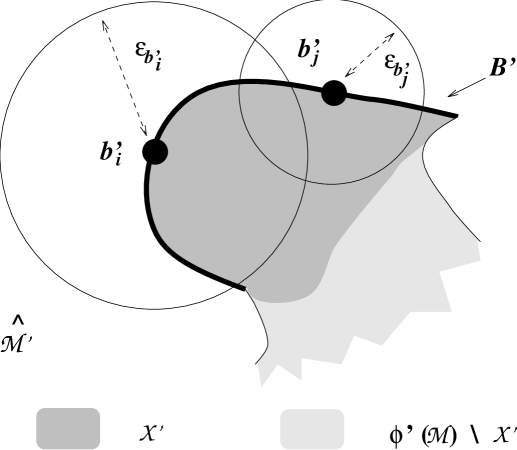
Figure 5: Illustrating the construction of ${\cal U}^{\prime}$ in the proof of Lemma 4.7.

To show necessity, let $B\rhd B^{\prime}$; i.e., for any open neighbourhood ${\cal U}$ of $B$ in ${\widehat{{\cal M}}}$, there is an open neighbourhood ${\cal V}^{\prime}$ of $B^{\prime}$ in ${\widehat{{\cal M}}}^{\prime}$ with

$$\phi\circ(\phi^{\prime})^{-1}({\cal V}^{\prime}\cap\phi^{\prime}({\cal M}))\subset{\cal U}.$$

Let $d^{\prime}$ be a Riemannian metric on ${\widehat{{\cal M}}}^{\prime}$ and let

$$X^{\prime}\mathop{=}\limits^{\hbox{\footnotesize def}}\phi^{\prime}\circ\phi^{-1}({\cal U}\cap\phi({\cal M})).$$

Now suppose that for some $b^{\prime}\in B^{\prime}$, there does not exist an $\epsilon_{b^{\prime}}>0$ such that $B_{d^{\prime}}(b^{\prime},\epsilon_{b^{\prime}})\cap\phi^{\prime}({\cal M})\subset X^{\prime}$. Thus a sequence $\{p_{n}\}$ of points of ${\cal M}$ can be found such that $\phi^{\prime}(p_{n})\not\in X^{\prime}$, but $\phi^{\prime}(p_{n})\mathop{\stackrel{{\scriptstyle n\to\infty}}{{\longrightarrow}}}b^{\prime}$. Since $B\rhd B^{\prime}$, by Theorem 19 of [5], $\{p_{n}\}$ admits a subsequence $\{p_{n_{i}}\}$ such that $\phi(p_{n_{i}})\mathop{\stackrel{{\scriptstyle i\to\infty}}{{\longrightarrow}}}b\in B$ for some $b$. So $\phi(p_{n_{i}})$ must eventually lie in ${\cal U}$ which contradicts that $\phi^{\prime}(p_{n_{i}})\not\in X^{\prime}$.

Thus for each $b^{\prime}\in B^{\prime}$, there exists an $\epsilon_{b^{\prime}}>0$ such that $B_{d^{\prime}}(b^{\prime},\epsilon_{b^{\prime}})\cap\phi^{\prime}({\cal M})\subset X^{\prime}$. (See Figure 5.) Define

$${\cal U}^{\prime}\mathop{=}\limits^{\hbox{\footnotesize def}}X^{\prime}\cup\biggl{(}\bigcup_{b^{\prime}\in B^{\prime}}B_{d^{\prime}}(b^{\prime},\epsilon_{b^{\prime}})\biggr{)}.$$

Then ${\cal U}^{\prime}$ is an open neighbourhood of $B^{\prime}$ satisfying the required property that

$$\phi\circ(\phi^{\prime})^{-1}({\cal U}^{\prime}\cap\phi^{\prime}({\cal M}))={\cal U}\cap\phi({\cal M}).$$

Using this equivalent formulation of “covering”, the main theorem can now be proven in a straightforward manner.

Theorem 4.9.

Let $T$ be a topological property. If $B$ satisfies the n$T$NP and $B\sim B^{\prime}$, then $B^{\prime}$ also satisfies the n$T$NP.

Proof 4.10.

Assume that $B$ satisfies the n$T$NP and $B\sim B^{\prime}$, but that $B^{\prime}$ does not satisfy the n$T$NP. This means that there is an open neighbourhood ${\cal U}^{\prime}$ of $B^{\prime}$ in ${\widehat{{\cal M}}}^{\prime}$ such that ${\cal U}^{\prime}$ contains no $T$-nice, open neighbourhoods of $B^{\prime}$. Since $B\lhd B^{\prime}$, there is an open neighbourhood ${\cal U}$ of $B$ in ${\widehat{{\cal M}}}$ such that

$$\phi^{\prime}\circ\phi^{-1}({\cal U}\cap\phi({\cal M}))\subset{\cal U}^{\prime}.$$ (2)

Since $B$ satisfies the n$T$NP, there is a $T$-nice, open neighbourhood ${\cal V}$ of $B$ contained in ${\cal U}$. By Lemma 4.7, since $B\rhd B^{\prime}$, there is an open neighbourhood ${\cal V}^{\prime}$ of $B^{\prime}$ with

$$\phi\circ(\phi^{\prime})^{-1}({\cal V}^{\prime}\cap\phi^{\prime}({\cal M}))={\cal V}\cap\phi({\cal M}).$$ (3)

Now define ${\cal W}^{\prime}\mathop{=}\limits^{\hbox{\footnotesize def}}({\cal V}^{\prime}\cap{\cal U}^{\prime})\cup({\cal V}^{\prime}\cap\phi^{\prime}({\cal M}))$. It is clear that ${\cal W}^{\prime}$ is an open neighbourhood of $B^{\prime}$, ${\cal W}^{\prime}\subset{\cal U}^{\prime}$, and ${\cal W}^{\prime}\cap\phi^{\prime}({\cal M})={\cal V}^{\prime}\cap\phi^{\prime}({\cal M})$.

Thus we have constructed an open neighbourhood ${\cal W}^{\prime}$ of $B^{\prime}$ which is contained in ${\cal U}^{\prime}$, and satisfies (3) with ${\cal V}^{\prime}$ replaced by ${\cal W}^{\prime}$. Since ${\cal V}$ is $T$-nice and $\phi^{\prime}\circ\phi^{-1}$ is a homeomorphism, it follows that ${\cal W}^{\prime}$ is $T$-nice. This is a contradiction, and the theorem is proven.

Corollary 4.11.

If $T$ is a topological property, then the n$T$NP is a well-defined property of abstract boundary sets $[B]$: we say that $[B]$ satisfies the n$T$NP if and only if the representative boundary set $B$ satisfies the n$T$NP.

Proof 4.12.

By Theorem 4.9, this definition is independent of the representative boundary set chosen.

Remark 4.13.

In particular, the n$T$NP passes to the abstract boundary ${\cal B}({\cal M})$.

For the moment we let $T={}$“connected”, and investigate the n$C$NP. First we find examples of connected boundary sets $B$ not satisfying the n$C$NP.

• Consider the isolated boundary set $B$ of Example 4.1. There, $B$ is connected, but is readily seen by inspection not to satisfy the n$C$NP.

  Alternatively, $B\sim B^{\prime}$, where $B^{\prime}$ consists of $g$ components and thus cannot satisfy the n$C$NP by Theorem 4.5. It then follows from Theorem 4.9 that $B$ cannot satisfy the n$C$NP either.

• In this example, the boundary set in question is non-compact, and thus not isolated. Let ${\widehat{{\cal M}}}={\mathbb{R}}\times S^{1}=\left\{\>(t,\theta)\mathbin{:}t\in{\mathbb{R}},-\pi<\theta\leq\pi\>\right\}$. Define ${\cal M}\mathop{=}\limits^{\hbox{\footnotesize def}}{\widehat{{\cal M}}}\setminus\{\theta=\pi\}$, and let $\phi$ be the inclusion. Then the boundary set $B=\partial_{\phi}=\{\theta=\pi\}$ is connected.

  Let ${\cal U}$ be an open neighbourhood of $B$, given by

  $${\cal U}\mathop{=}\limits^{\hbox{\footnotesize def}}\left\{\>(t,\theta)\mathbin{:}t\in{\mathbb{R}},-\pi<\theta<-a\hbox{ or }a<\theta\leq\pi\>\right\},$$

  where $0<a<\pi$. Then ${\cal U}\cap\phi({\cal M})$ has precisely two components. Furthermore, for any open neighbourhood ${\cal V}$ of $B$ contained in ${\cal U}$, ${\cal V}\cap\phi({\cal M})$ must have at least two components. Thus $B$ does not satisfy the n$C$NP.

  We note that a similar argument to that used at the end of Example (i) could be used here. If ${\widehat{{\cal M}}}^{\prime}={\widehat{{\cal M}}}$ and $\phi^{\prime}$ maps $(t,\theta)$ to $(t^{\prime},\theta^{\prime})=(t,\theta/2)$, then

  $$B^{\prime}=\partial_{\phi^{\prime}}=\{\theta^{\prime}=-\pi/2\}\cup\{\theta^{\prime}=\pi/2\}$$

  is the union of two components, and $B^{\prime}\sim B$.

4.3 Isolated boundary points and the n$C$NP

We now show that, for $n\geq 2$, all boundary sets equivalent to an isolated boundary point must satisfy the n$C$NP. There are, of course, many other types of boundary point which satisfy the n$C$NP—for specific examples this question is often easily settled by inspection.

In the following one wishes to talk about balls of certain radii about an isolated boundary point, so again we fix a Riemannian metric $d$ for ${\widehat{{\cal M}}}$.

Lemma 4.14.

Let $n\geq 2$. If $p$ is an isolated boundary point then, for some $\epsilon>0$, there is an open metric ball $B_{\epsilon}$ about $p$, of radius $\epsilon$, which intersects $\partial_{\phi}$ at n(and only atn) $p$, and is such that $B_{\epsilon}\setminus\{p\}\subset\phi({\cal M})$. It follows that, if $n\geq 2$, an isolated boundary point satisfies the n$C$NP.

Proof 4.15.

Since $p$ is an isolated boundary point, there is an open neighbourhood ${\cal U}$ of $p$ in ${\widehat{{\cal M}}}$ such that ${\cal U}\cap\partial_{\phi}=\{p\}$. Let $B_{\epsilon}\mathop{=}\limits^{\hbox{\footnotesize def}}B_{d}(p,\epsilon)$ be an open $d$-ball about $p$ with radius $\epsilon>0$, such that $B_{\epsilon}\subset{\cal U}$. Clearly $B_{\epsilon}\cap\partial_{\phi}=\{p\}$.

For $n\geq 2$, $B_{\epsilon}\setminus\{p\}$ is connected. We already know that $(B_{\epsilon}\setminus\{p\})\cap\partial_{\phi}=\emptyset$, and $X\mathop{=}\limits^{\hbox{\footnotesize def}}(B_{\epsilon}\setminus\{p\})\cap\phi({\cal M})\neq\emptyset$, since $p$ is a boundary point and so must be a limit point of a sequence of points in $\phi({\cal M})$. Also, $X$ is open in the relative topology of $B_{\epsilon}\setminus\{p\}$, since $\phi({\cal M})$ is open.

Suppose that $Y\mathop{=}\limits^{\hbox{\footnotesize def}}(B_{\epsilon}\setminus\{p\})\cap({\widehat{{\cal M}}}\setminus\overline{\phi({\cal M})})\neq\emptyset$. It is readily seen that $Y$ is also open in the relative topology of $B_{\epsilon}\setminus\{p\}$, since ${\widehat{{\cal M}}}\setminus\overline{\phi({\cal M})}$ is open. This yields a contradiction, since $B_{\epsilon}\setminus\{p\}=X\cup Y$ is the disjoint union of two non-empty open sets, yet it is connected. It follows that $B_{\epsilon}\setminus\{p\}\subset\phi({\cal M})$.

For all open $d$-balls $B_{\mu}\mathop{=}\limits^{\hbox{\footnotesize def}}B_{d}(p,\mu)$, $0<\mu<\epsilon$, it is clear that $B_{\mu}\setminus\{p\}$ is a subset of $\phi({\cal M})$ and is connected. Since any open neighbourhood of $p$ in ${\widehat{{\cal M}}}$ contains such a ball, it follows that $\{p\}$ satisfies the n$C$NP.

Corollary 4.16.

If $n\geq 2$, an isolated abstract boundary point $[p]$ satisfies the n$C$NP. Every boundary set $B\in[p]$ is thus connected.

Proof 4.17.

This follows immediately from Lemma 4.14, Corollary 4.11, and Theorem 4.5.

Example 4.18.

Lemma 4.14 fails trivially for $n=1$, since if ${\cal M}={\mathbb{R}}$, ${\widehat{{\cal M}}}=S^{1}=\left\{\>\theta\mathbin{:}-\pi<\theta\leq\pi\>\right\}$ and $\phi(t)=2\arctan t$, then the boundary point $p$ ($\{p\}=\partial_{\phi}$) given by $\theta=\pi$ is isolated, yet clearly does not satisfy the n$C$NP.

We close this section with an answer to a question posed in [5].

Example 4.19.

We now can find immediately an example of an equivalence class of compact boundary sets which is not an abstract boundary point, answering a question of [5] in the negative. Simply take the equivalence class containing an isolated boundary set with more than one component (examples of such are very easy to come by: e.g., excise two disjoint closed discs from a plane ${\widehat{{\cal M}}}={\mathbb{R}}^{2}$ to obtain ${\cal M}$). For $n\geq 2$, such a set cannot be equivalent to a point: by Theorem 3.4 this point would be isolated, whence all boundary sets equivalent to it would be connected (Corollary 4.16).

5 Simple connectedness and vanishing of higher homotopy groups

Theorem 4.9 can be used for many different topological properties $T$, in addition to $T=C$ (which was examined in detail in §4). Consider the following few examples.

• $T(X)={}$“$X$ is simply connected”${}\mathop{=}\limits^{\hbox{\footnotesize def}}SC(X)$.

• $T(X)={}$“$H_{k}(X)$ is the trivial group”${}\mathop{=}\limits^{\hbox{\footnotesize def}}HOM_{k}(X)$, $k\in{\mathbb{Z}},0\leq k\leq n$.

• Since we are interested in neighbourhood properties of subsets $B$ of a manifold, then the intersection $X$ of an open neighbourhood of $B$ with $\phi({\cal M})$ is itself a manifold, although not necessarily a connected one. Thus we may let $T(X)={}$“$X$ is parallelisable”. Recall that a differentiable manifold $X$ is called parallelisable if the frame bundle $LX$ of $X$ admits a nowhere-vanishing (continuous) section. If $X$ has a pseudo-Riemannian metric, this is the condition that $X$ admit a globally defined, nowhere-vanishing, continuous orthonormal field.

• $T(X)={}$“$X$ is $k$-connected”${}\mathop{=}\limits^{\hbox{\footnotesize def}}\Pi_{k}(X)$, $k\in{\mathbb{Z}},k\geq 1$.

(Note that $\Pi_{1}(X)$ is, of course, the same as $SC(X)$, and $HOM_{0}(X)$ is the same as $C(X)$.) Thus we have defined the n$SC$NP, $\Pi_{k}$nNP and $HOM_{k}$nNP of boundary sets. Corollary 4.11, of course, shows that all of the above neighbourhood properties—the n$C$NP, n$SC$NP and $\Pi_{k}$nNP for $k\geq 1$, in particular—are well-defined properties of abstract boundary sets.

Rather than catalogue a large list of topological properties in detail, in this section we shall just consider the situation where $T=SC$. Since it involves hardly any more effort, we will seek to generalise some of our results to the case where $T=\Pi_{k}$, $k\geq 1$.

We begin by examining the issue of the simple connectedness of the boundary sets themselves (§5.1), then proceed to consider boundary sets which satisfy the n$SC$NP (§5.2).

5.1 Simply connected boundary sets

We immediately note that, just as in the case of connectedness, it may easily be seen that simple connectedness does not pass to abstract boundary sets (including abstract boundary points, i.e., members of the a-boundary). We present here two examples of non-simply-connected boundary sets that are equivalent to boundary points. In the first example the boundary sets involved are not isolated, whereas in the second example they are isolated.

• 

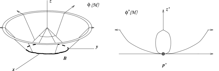
  Figure 6: An illustration of Example (i). On the left is depicted ${\cal M}=\phi({\cal M})\subset{\widehat{{\cal M}}}$, and on the right is shown a cross-section of $\phi^{\prime}({\cal M})$, through a plane containing the $z^{\prime}$-axis. The boundary sets $B$ and $\{p^{\prime}\}$ are equivalent.

  Let $f:{\mathbb{R}}^{+}\cup\{0\}\to{\mathbb{R}}$ (the domain is the non-negative reals) be the map

  $$x\mapsto\cases{1-x,&for $0\leq x\leq 1$,\cr x-1,&for $1<x<2$,\cr 1,&otherwise.\cr}$$

  Introduce cylindrical polar coordinates $r,\theta,z$ on ${\mathbb{R}}^{3}\setminus{}z$-axis. Let ${\cal M}$ be the subset of ${\mathbb{R}}^{3}\setminus{}z$-axis defined by

  $${\cal M}\mathop{=}\limits^{\hbox{\footnotesize def}}\{\>(r,\theta,z)\>\colon\>z>f(r)\>\}$$

  (see Figure 6). Let ${\widehat{{\cal M}}}={\widehat{{\cal M}}}^{\prime}\mathop{=}\limits^{\hbox{\footnotesize def}}{\mathbb{R}}^{3}$, let $\phi$ be the inclusion, and let

  $$\phi^{\prime}:{\cal M}\to{\widehat{{\cal M}}}^{\prime}\qquad\hbox{be given by}\qquad(r,\theta,z)\mapsto(r^{\prime},\theta^{\prime},z^{\prime})=(zr,\theta,z).$$

  This map is smooth and has Jacobian $z$, which vanishes nowhere on ${\cal M}$. It is thus immersive on ${\cal M}$. By the Inverse Function Theorem (or by inspection), its inverse $\phi^{\prime}({\cal M})\to{\cal M}:(r^{\prime},\theta^{\prime},z^{\prime})\mapsto(r,\theta,z)=(r^{\prime}/z^{\prime},\theta^{\prime},z^{\prime})$ is also smooth.

  Let $B=\left\{\>(1,\theta,0)\mathbin{:}0\leq\theta<2\pi\>\right\}\subset\partial_{\phi}$ and $p^{\prime}=(0,0,0)\in\partial_{\phi^{\prime}}$. It is readily seen that $B\sim p^{\prime}$, but $B$ is homeomorphic to $S^{1}$.

  This example admits generalisation to higher dimensions, in the same manner as at the end of Example 4.1.

  Thus, for any dimension $n\geq 3$, a boundary point can be equivalent to a non-simply-connected boundary set. In particular, simple connectedness does not pass to the a-boundary.

• Consider Example 15 of [5]. There ${\widehat{{\cal M}}}={\widehat{{\cal M}}}^{\prime}={\mathbb{R}}^{n}$, for some integer $n\geq 2$. We introduce spherical polar coordinates $r,\hbox{$\theta_{1},\ldots,\theta_{n-1}$}$, on the manifold ${\cal M}\mathop{=}\limits^{\hbox{\footnotesize def}}{\mathbb{R}}^{n}\setminus\{{\mathbb{0}}\}\approx{\mathbb{R}}^{+}\times S^{n-1}$. Let $\phi$ be the inclusion, and $\phi^{\prime}$ be the map

  $$(r,\hbox{$\theta_{1},\ldots,\theta_{n-1}$})\mapsto(r^{\prime},\hbox{$\theta^{\prime}_{1},\ldots,\theta^{\prime}_{n-1}$})=(r+1,\hbox{$\theta_{1},\ldots,\theta_{n-1}$}).$$

  Then let $B^{\prime}\mathop{=}\limits^{\hbox{\footnotesize def}}\partial_{\phi^{\prime}}=\{r^{\prime}=1\}\approx S^{n-1}$, and let $p$ be the origin ${\mathbb{0}}\in{\widehat{{\cal M}}}$. Both $B^{\prime}$ and $\{p\}$ are isolated boundary sets.

  We clearly have $B^{\prime}\sim p$, yet for $n=2$, $B^{\prime}\approx S^{1}$ is not simply connected. (Indeed, $\pi_{n-1}(B^{\prime})$ is non-trivial for any integer $n\geq 2$.)

5.2 The simply connected neighbourhood property

Although we have seen (Corollary 4.16, Example 4.19) that, for $n\geq 2$, no disconnected, isolated boundary set is equivalent to a boundary point, it is of interest to ask whether some connected, isolated boundary sets have the property that they are not equivalent to any boundary point. We show here that there are indeed examples of this kind of boundary set. In particular, we next give an example of a connected, isolated boundary set, failing to satisfy the n$SC$NP, which is equivalent to no boundary point. In fact, for $n\geq 3$, an isolated boundary set which fails to satisfy the n$SC$NP is never equivalent to a boundary point. (We shall delay the proof of this result until Corollary 5.5.)

Example 5.1.

Let ${\cal M}={\mathbb{R}}^{3}\setminus B$, where $B$ is a homeomorph of $S^{1}$: say $B=\{x^{2}+y^{2}=1,z=0\}$. Let ${\widehat{{\cal M}}}={\mathbb{R}}^{3}$ and $\phi$ be the inclusion, so that $\partial_{\phi}=B$ is a non-simply connected, connected, isolated boundary set.

We claim that $B$ does not satisfy the n$SC$NP. Indeed, it is easy to see that any open neighbourhood ${\cal U}$ of $B$ contains an open neighbourhood of the form

$${\cal W}_{\eta}\mathop{=}\limits^{\hbox{\footnotesize def}}\bigcup_{b\in B}B_{d}(b,\eta),$$

for some $0<\eta\leq 1$, where $d$ is the usual Euclidean metric on ${\mathbb{R}}^{3}$. For $0<\eta\leq 1$, the image of the loop

$$\gamma_{\eta}:[0,1]\to{\mathbb{R}}^{3}:t\mapsto(1-\eta/2)(\cos 2\pi t,\sin 2\pi t,0)$$

is contained in ${\cal W}_{\eta}\setminus B={\cal W}_{\eta}\cap\phi({\cal M})$. For any $0<\eta\leq 1$, the loop $\gamma_{\eta}$ is clearly not homotopic to a constant map in ${\cal W}_{\eta}\setminus B={\cal W}_{\eta}\cap\phi({\cal M})$; indeed, neither is $\gamma_{\eta}$ homotopic to a constant map in ${\cal W}_{1}\setminus B={\cal W}_{1}\cap\phi({\cal M})$. No open neighbourhood ${\cal V}$ of $B$, contained in ${\cal W}_{1}$, can be $SC$-nice: were it so, there would be some $0<\eta^{\ast}<1$ for which ${\cal W}_{\eta^{\ast}}\subset{\cal V}$, and the loop $\gamma_{\eta^{\ast}}$ would be homotopic to a constant map in ${\cal V}\setminus B={\cal V}\cap\phi({\cal M})\subset{\cal W}_{1}\cap\phi({\cal M})$. This would be a contradiction, so that ${\cal W}_{1}$ contains no $SC$-nice, open neighbourhoods of $B$. This means that $B$ does not satisfy the n$SC$NP.

Let $p^{\prime}$ be an isolated boundary point of an envelopment $({\cal M},{\widehat{{\cal M}}}^{\prime},\phi^{\prime})$. We claim that $p^{\prime}$ always satisfies the n$SC$NP. Fix a Riemannian metric $d^{\prime}$ for ${\widehat{{\cal M}}}^{\prime}$, and define open balls $B^{\prime}_{\epsilon}\mathop{=}\limits^{\hbox{\footnotesize def}}B_{d^{\prime}}(p^{\prime},\epsilon)$, as in Lemma 4.14. It follows, by the same lemma, that for $\epsilon$ sufficiently small we have $B^{\prime}_{\epsilon}\cap\phi^{\prime}({\cal M})=B^{\prime}_{\epsilon}\setminus\{p^{\prime}\}$, and that this set $B^{\prime}_{\epsilon}\cap\phi^{\prime}({\cal M})$ is homeomorphic to a ball $E^{3}$ without its centre. Hence $B^{\prime}_{\epsilon}\cap\phi^{\prime}({\cal M})$ is homotopic to a 2-sphere, and is thereby simply connected. It follows that $p^{\prime}$ satisfies the n$SC$NP.

By Theorem 4.9, we have $B\not\sim p^{\prime}$, where $p^{\prime}$ is any isolated boundary point. Theorem 3.4 tells us, however, that any boundary point equivalent to $B$ must be isolated, so that $B$ cannot be equivalent to any boundary point; in other words, $[B]\not\in{\cal B}({\cal M})$.

We know that a boundary set $B$ may be simply connected, yet fail to satisfy the n$C$NP (Example (ii) is an example of this, wherein the set $B$ is both connected and simply connected). Such a set, then, cannot satisfy the n$SC$NP. A simply connected boundary set may fail the n$SC$NP for more subtle reasons than this, however—i.e., it is possible to find simply connected boundary sets which satisfy the n$C$NP, yet which fail the n$SC$NP. One example of this is the boundary point $p^{\prime}$ of Example (i).

We now complete our demonstration that the notions of simple connectedness of boundary sets, on the one hand, and the n$SC$NP of boundary sets, on the other, are logically independent. To this end, we will show in the next example that a boundary set $B$ may satisfy the n$SC$NP, yet fail to be simply connected, itself. This means we cannot find an analogue of Theorem 4.5 for simple connectedness, and demonstrates the difficulty of finding criteria which ensure the invariance of simple connectedness of boundary sets under boundary set equivalence.

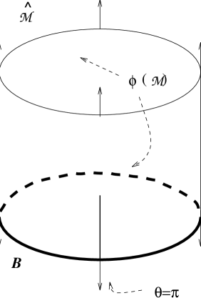
Figure 7: An illustration of Example 5.2, in which $B$ satisfies the n$SC$NP but is not simply connected.

Example 5.2.

Let ${\widehat{{\cal M}}}$ be a cylinder

$${\widehat{{\cal M}}}\mathop{=}\limits^{\hbox{\footnotesize def}}{\mathbb{R}}\times S^{1}=\left\{\>(t,\theta)\mathbin{:}-\infty<t<\infty,-\pi<\theta\leq\pi\>\right\}.$$

Let ${\cal M}\subset{\widehat{{\cal M}}}$ be the region

$$\left\{\>(t,\theta)\in{\widehat{{\cal M}}}\mathbin{:}t>0,\theta\neq\pi\hbox{ if }t\leq 1\>\right\},$$

and let $\phi$ be the inclusion—see Figure 7. So $\partial_{\phi}=B\cup\left\{\>(t,\pi)\mathbin{:}0<t\leq 1\>\right\}$, where $B$ is the circle $B\mathop{=}\limits^{\hbox{\footnotesize def}}\left\{\>(0,\theta)\mathbin{:}-\pi<\theta\leq\pi\>\right\}$. It is easy to see that $B$, which is not simply connected, satisfies the n$SC$NP.

This example admits generalisation to higher dimensions, in the same manner as at the end of Example 4.1, but here the manifold $X_{0}$ should be simply connected. Thus, for any dimension $n\geq 2$, we have an example of a boundary set which is not simply connected, yet which satisfies the n$SC$NP. (In §6 we shall show that, since $B$ is also a differentiable submanifold of ${\widehat{{\cal M}}}$ admitting a nowhere-vanishing normal vector field, this pathology occurs only because $B$ fails to be isolated.)

5.3 Isolated boundary points and the $\Pi_{k}$nNP

When $n\geq 3$, we can prove that there are no isolated boundary points (and thus no isolated abstract boundary points) which fail the n$SC$NP. We can say considerably more than this, however.

Theorem 5.3.

Let $k$ be a positive integer, and assume that the dimension $n$ of ${\cal M}$ satisfies $n\geq k+2$. Then an isolated boundary point satisfies the $\Pi_{k}$nNP. Thus, if $n\geq k+2$, a boundary set which does not satisfy the $\Pi_{k}$nNP is not equivalent to any isolated boundary point.

Proof 5.4.

Let $p$ be an isolated boundary point of the envelopment $({\cal M},{\widehat{{\cal M}}},\phi)$, and equip ${\widehat{{\cal M}}}$ with a Riemannian metric $d$. By Lemma 4.14, for some $\epsilon>0$, there is an open metric ball $B_{\epsilon}\mathop{=}\limits^{\hbox{\footnotesize def}}B_{d}(p,\epsilon)$ about $p$, of radius $\epsilon$, which intersects $\partial_{\phi}$ at (and only at) $p$, and is such that $B_{\epsilon}\setminus\{p\}\subset\phi({\cal M})$. Similarly, for all $\mu$ where $0<\mu<\epsilon$, we let $B_{\mu}\mathop{=}\limits^{\hbox{\footnotesize def}}B_{d}(p,\mu)$. We have $B_{\mu}\cap\partial_{\phi}=\{p\}$ and $B_{\mu}\setminus\{p\}\subset\phi({\cal M})$. Now each $B_{\mu}\setminus\{p\}$ is homeomorphic to a ball without its centre, $E^{n}\setminus\{{\mathbb{0}}\}$. Thus each $B_{\mu}\setminus\{p\}$ has the homotopy type of a sphere $S^{n-1}$. Since $\pi_{k}(S^{n-1})$ is trivial for $k<n-1$, it follows that $\{p\}$ satisfies the $\Pi_{k}$nNP when $n\geq k+2$. This proves the first statement of the theorem.

The second sentence is immediate. Assume that $B$ is an isolated boundary set which is equivalent to a boundary point $p^{\prime}$. Then $p^{\prime}$ is isolated, by Theorem 3.4, whence it satisfies the $\Pi_{k}$nNP, for $n\geq k+2$. Thus $B$ also satisfies the $\Pi_{k}$nNP, by Corollary 4.11.

Since n$SC$NP${}\equiv\Pi_{1}$NP, we have the following corollary as an example of this theorem.

Corollary 5.5.

If $n\geq 3$, then any isolated boundary point satisfies the n$SC$NP. Thus, if $n\geq 3$, a boundary set which does not satisfy the n$SC$NP is not equivalent to any isolated boundary point.

Remarks.

1. If $n=k+1$ then the result of Theorem 5.3 is not true. To see this, let ${\widehat{{\cal M}}}={\mathbb{R}}^{k+1}={\widehat{{\cal M}}}^{\prime}$, and ${\cal M}=\phi({\cal M})={\mathbb{R}}^{k+1}-\{p\}$ ($\phi={}$inclusion), where $p$ is the origin $(0,\ldots,0)$. Let $\phi^{\prime}$, in spherical polar coordinates, be the map $(r,\hbox{$\theta_{1},\ldots,\theta_{k}$})\mapsto(r+1,\hbox{$\theta_{1},\ldots,\theta_{k}$})$ as in Example (ii). Then $p$, an isolated boundary point, is equivalent to a $k$-dimensional sphere $B^{\prime}\approx S^{k}$. There is a base $\{{\cal U}^{\prime}_{A}\}$ of neighbourhoods of $B^{\prime}$ in ${\widehat{{\cal M}}}^{\prime}$, such that each ${\cal U}^{\prime}_{A}\cap\phi^{\prime}({\cal M})$ is homeomorphic to $S^{k}\times(0,1)$, and

   $$\pi_{k}(S^{k}\times(0,1))\approx\pi_{k}(S^{k})\times\pi_{k}((0,1))\approx{\mathbb{Z}}.$$

   Hence no ${\cal U}^{\prime}_{A}\cap\phi^{\prime}({\cal M})$ is $k$-connected, and it follows that $B^{\prime}$, and thus $p$, does not satisfy the $\Pi_{k}$nNP.

2. The (integral) homology groups of the sphere $S^{n-1}$ are

   $$H_{i}(S^{n-1})\approx\cases{0,&if $i\neq 0,n-1$,\cr{\mathbb{Z}},&if $i=0$ or $i=n-1$,\cr}\qquad 0\leq i\leq n-1.$$

   Upon examining the proof of Theorem 5.3, it is easily seen that one can replace the $\Pi_{k}$nNP with the $HOM_{k}$nNP in the statement of that theorem, to obtain a new result. To do this, we need conditions on $k$ and $n$ that will ensure the triviality of $H_{k}(S^{n-1})$, and clearly the condition $1\leq k\leq n-2$ suffices. Thus we have the following result.

   Theorem 5.6.

   Let $k$ be a positive integer, satisfying $1\leq k\leq n-2$, where $n$ is the dimension of ${\cal M}$. Then an isolated boundary point satisfies the $HOM_{k}$nNP. Thus, if $1\leq k\leq n-2$, a boundary set which does not satisfy the $HOM_{k}$nNP is not equivalent to any isolated boundary point.

6 An application to isolated boundary submanifolds

Note that Theorem 5.3 and Corollary 5.5 do not directly help us in deciding whether a boundary set $B$, which fails to be simply connected itself (or is not $k$-connected, for some $k>1$), can be equivalent to an isolated boundary point. In this section we seek conditions on $B$ that will allow us to answer such a question.

Definition 6.1.

A boundary set $B$ of an envelopment $({\cal M},{\widehat{{\cal M}}},\phi)$, which is also a differentiable submanifold of ${\widehat{{\cal M}}}$, will be called a boundary submanifold. If $B$ is also of codimension 1 in ${\widehat{{\cal M}}}$, it will be called a boundary hypersurface.

We will show that isolated boundary submanifolds $B$, which fail to be $k$-connected (i.e., which have non-trivial $k$th homotopy group), and also obey a fairly easily checked criterion, fail to satisfy the $\Pi_{k}$nNP. Thus, such a $B$ cannot be equivalent to a boundary set satisfying the $\Pi_{k}$nNP. In particular, if $n\geq k+2$, $B$ cannot be equivalent to a (necessarily isolated) boundary point.

In considering an isolated boundary submanifold $B$ of codimension $\ell>1$, one might hope to find open neighbourhoods of $B$ homeomorphic to a product $B\times E^{\ell}$, with $B$ carried onto $B\times\{{\mathbb{0}}\}$. Unfortunately, such neighbourhoods do not exist in general. The problem is to do with the possible non-triviality of the normal bundle of a submanifold. To deal with this we use more general neighbourhoods called “tubular neighbourhoods”. (In Appendix A, we give a few definitions that may be of use to those unfamiliar with some of the following terminology.)

Definition 6.2.

Let ${\cal V}$ be a smooth manifold, and let ${\cal M}\subset{\cal V}$ be a differentiable submanifold. A tubular neighbourhood of ${\cal M}$ (or for $({\cal V},{\cal M})$) is a pair $(f,\xi)$, where $\xi=(p,E,{\cal M})$ is a vector bundle over ${\cal M}$ and $f:E\to{\cal V}$ is an embedding such that

1. $f|_{\cal M}={}$the identity on ${\cal M}$, where ${\cal M}$ is identified with the zero section of $\xi$;

2. $f(E)$ is an open neighbourhood of ${\cal M}$ in ${\cal V}$.

We often simply refer to ${\cal W}=f(E)$ as a tubular neighbourhood of ${\cal M}$. To ${\cal W}$ is associated a retraction $q:{\cal W}\to{\cal M}$, making $(q,{\cal W},{\cal M})$ a vector bundle, isomorphic to $\xi$, whose zero section is the inclusion ${\cal M}\subset{\cal V}$.

When $\xi$ is the normal bundle of ${\cal M}$ in ${\cal V}$, ${\cal W}$ is called a normal tubular neighbourhood.

Note that differentiability of all manifolds is required in the above definition, since one requires $f$ to be an embedding.

We now state the very powerful Tubular Neighbourhood Theorem.

Theorem 6.3 ([3, Theorem 4.5.2]).

Any differentiable submanifold ${\cal N}$ of a differentiable manifold ${\cal M}$ has a tubular neighbourhood $(f,\xi)$ n(or ${\cal W}$n). Furthermore, $(f,\xi)$ can be chosen so that $\xi$ is the normal bundle of ${\cal N}$, with respect to any Riemannian metric on ${\cal M}$.

In fact, by “retracting along the fibres” of any tubular neighbourhood and, in particular, any normal tubular neighbourhood, we see that the collection of normal tubular neighbourhoods of ${\cal N}$ forms a base for the neighbourhood system of ${\cal N}$.

Using normal tubular neighbourhoods, we can relate the condition of $k$-connectedness of an isolated boundary submanifold $B$, to the $\Pi_{k}$nNP for $B$.

Theorem 6.4.

Let $B$ be a connected, isolated boundary submanifold of the envelopment $({\cal M},{\widehat{{\cal M}}},\phi)$. Fix any Riemannian structure on ${\widehat{{\cal M}}}$, with respect to which the normal bundle $NB$ of $B$ is defined. Assume that there is a section of the normal bundle $NB$ of $B$ in ${\widehat{{\cal M}}}$ which does not vanish at any point of $B$. If $B$ is not $k$-connected, then $B$ does not satisfy the $\Pi_{k}$nNP.

Proof 6.5.

Let $\sigma:B\to NB$ be a nowhere-vanishing section of $NB$. Since $B$ is isolated, there is a neighbourhood ${\cal U}$ of $B$ in ${\widehat{{\cal M}}}$ such that ${\cal U}\cap\partial_{\phi}=B$. Let ${\cal W}$ be a normal tubular neighbourhood of $B$ contained in ${\cal U}$ (c.f. Theorem 6.3), with projection $q:{\cal W}\to B$, and let $f:NB\to{\cal W}$ be an embedding, as in the definition of tubular neighbourhoods. We will use the map $f\circ\sigma$ to “lift” a map $\lambda:S^{k}\to B$ to a map $S^{k}\to{\cal W}\cap\phi({\cal M})$. Before doing this, though, we must check that $\sigma$ “points into $\phi({\cal M})$”, and replace it if this is not the case.

First, let us assume that the codimension of $B$ in ${\widehat{{\cal M}}}$ is greater than one. Now each point $p$ of $B$ has a neighbourhood $X_{p}\subset{\cal W}$ homeomorphic to ${\mathbb{R}}^{n}$, with $B\cap X_{p}$ corresponding to a linear subspace $V\subset{\mathbb{R}}^{n}$ of dimension $m\leq n-2$. We claim that ${\mathbb{R}}^{n}\setminus V$ is connected. Non-singular linear transformations of ${\mathbb{R}}^{n}$ are homeomorphisms, whence we may assume that $V=\{{\mathbb{x}}=(\hbox{$x_{1},\ldots,x_{n}$})\in{\mathbb{R}}^{n}\>:\>x_{m+1}=\cdots=x_{n}=0\}$. The claim is then obvious, and thus $X_{p}\setminus B\approx{\mathbb{R}}^{n}\setminus V$ is connected. From this it follows that $\bigcup_{p\in B}(X_{p}\setminus B)$, being the union of connected, open sets, none of which is disjoint from all the others (since $B$ is connected), is also connected, whereby it is contained in $\phi({\cal M})$ (c.f. the proof of Lemma 4.14). Finally, we “normalise” $\sigma$ in the following manner. We can easily construct a smooth $t:B\to{\mathbb{R}}^{+}$ such that $f\circ[t(p)\cdot\sigma(p)]\in X_{p}\setminus B$, for all $p\in B$ (recall that $\sigma$ is nowhere-vanishing). Then the section $t\cdot\sigma$ (defined as the map $p\mapsto t(p)\cdot\sigma(p)$) satisfies $f\circ(t\cdot\sigma)\circ\lambda(S^{k})\subset{\cal W}\cap\phi({\cal M})$. We replace $\sigma$ with $t\cdot\sigma$.

It remains to consider the case where the codimension of $B$ in ${\widehat{{\cal M}}}$ is precisely one, i.e., where $B$ is a boundary hypersurface. In a similar manner to the argument of the previous paragraph, we note that each point $p$ of $B$ has a neighbourhood $X_{p}\subset{\cal W}$ homeomorphic to ${\mathbb{R}}^{2}$, with $B\cap X_{p}$ corresponding to an axis ${\mathbb{R}}$. We can also choose the homeomorphisms so that $X_{p}\cap\phi({\cal M})$ either corresponds to ${\mathbb{R}}^{2}\setminus x$-axis, or to the (open) upper half-plane.

As before, we can “normalise” $\sigma$ so that $f\circ\sigma(B)\subset\bigcup_{p\in B}(X_{p}\setminus B)$. Now at any point $p\in B$, either $f\circ\sigma(p)\in X_{p}\cap\phi({\cal M})$ or $f\circ(-\sigma)(p)\in X_{p}\cap\phi({\cal M})$ (or both are true), where $-\sigma\mathop{=}\limits^{\hbox{\footnotesize def}}-1\cdot\sigma$. If only the latter option is true, then we replace $\sigma$ with $-\sigma$ (this corresponds to swapping the “inward” or “outward” character of the “normal field” $\sigma$). It now follows, since the image $f\circ\sigma\circ\lambda(S^{k})$ is a connected subset of ${\cal W}$, and since $f\circ\sigma(p)\in\phi({\cal M})$ for any $p\in B$ (and, in particular, for $p\in\mathop{\operator@font Im}\nolimits\lambda$), that $f\circ\sigma\circ\lambda(S^{k})\subset{\cal W}\cap\phi({\cal M})$.

In both these cases, then, we may assume that $f\circ\sigma\circ\lambda(S^{k})\subset{\cal W}\cap\phi({\cal M})$ (i.e., this assumption is valid, regardless of the codimension of $B$ in ${\widehat{{\cal M}}}$).

Since $\pi_{k}(B)$ is non-trivial, there is a map $\lambda:S^{k}\to B$ which is not homotopic to a constant map. Consider the map $\lambda^{\prime}:S^{k}\to{\cal W}\cap\phi({\cal M})$ defined by

$$\lambda^{\prime}\mathop{=}\limits^{\hbox{\footnotesize def}}f\circ\sigma\circ\lambda.$$

Were $\lambda^{\prime}$ homotopic to a constant map in ${\cal W}\cap\phi({\cal M})$, such a homotopy

$$F:S^{k}\times I\to{\cal W}\cap\phi({\cal M}),\qquad F(\,\cdot\,,0)=\lambda^{\prime}(\,\cdot\,),\qquad F(\,\cdot\,,1)=w_{0}\in{\cal W}\cap\phi({\cal M}),$$

would give rise to a homotopy

$$q\circ F:S^{k}\times I\to B,\qquad q\circ F(\,\cdot\,,0)=\lambda(\,\cdot\,),\qquad q\circ F(\,\cdot\,,1)=q(w_{0}).$$

This would be a contradiction, since we assumed that $\lambda$ was not homotopic to a constant map. Thus the “lift” $\lambda^{\prime}$ cannot be homotopic to a constant map in ${\cal W}\cap\phi({\cal M})$.

We have now established most of the machinery necessary for the proof. To proceed, let us assume that $B$ satisfies the $\Pi_{k}$nNP, and attempt to derive a contradiction. Let ${\cal W}_{0}$ be a normal tubular neighbourhood of $B$ as in the above paragraphs (with $q_{0}:{\cal W}_{0}\to B$ the projection, and $f_{0}:NB\to{\cal W}_{0}$ an embedding, as in the definition of tubular neighbourhoods). Consider the “lift” $\lambda^{\prime}_{0}\mathop{=}\limits^{\hbox{\footnotesize def}}f_{0}\circ\sigma\circ\lambda$. Since $B$ satisfies the $\Pi_{k}$nNP, ${\cal W}_{0}$ contains an open $\Pi_{k}$-nice neighbourhood ${\cal V}$ of $B$. Now ${\cal V}$ contains a normal tubular neighbourhood ${\cal W}_{1}$ of $B$, with projection $q_{1}:{\cal W}_{1}\to B$, and with embedding $f_{1}:NB\to{\cal W}_{1}$. We may assume that ${\cal W}_{1}$ is obtained by “shrinking” ${\cal W}_{0}$: to be more specific, $f_{0}\circ{f_{1}}^{-1}:{\cal W}_{1}\to{\cal W}_{0}$ restricts on each fibre (which has the structure of a vector space) to be a dilatation—see Figure 8.

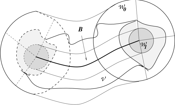
Figure 8: An illustration for the proof of Theorem 6.4. Here ${\cal V}$ is $\Pi_{k}$-nice, ${\cal W}_{0}$ and ${\cal W}_{1}$ are normal tubular neighbourhoods of $B$, and ${\cal W}_{1}\subset{\cal V}\subset{\cal W}_{0}$.

Consider $\lambda^{\prime}_{1}\mathop{=}\limits^{\hbox{\footnotesize def}}f_{1}\circ\sigma\circ\lambda$, which satisfies $\lambda_{1}^{\prime}(S^{k})\subset{\cal V}\cap\phi({\cal M})$. By our assumption on the relationship between ${\cal W}_{1}$ and ${\cal W}_{0}$ at the end of the previous paragraph, we have that $\lambda_{1}^{\prime}$ and $\lambda_{0}^{\prime}$ are homotopic in ${\cal W}_{0}$. Hence $\lambda_{1}^{\prime}$ is not homotopic to a constant map in ${\cal W}_{0}\cap\phi({\cal M})$, and it follows that it cannot be so in ${\cal V}\cap\phi({\cal M})$. This is a contradiction because we assumed that ${\cal V}$ is $\Pi_{k}$-nice, and the result is established.

In the above proof, the condition that $NB$ have a nowhere-vanishing section is a convenient tool for “lifting” a map $S^{k}\to B$ to a map from $S^{k}$ to ${\cal W}\cap\phi({\cal M})$, where ${\cal W}$ is a normal tubular neighbourhood of $B$. This condition should be easily verified (if true), for specific examples—especially when $B$ is contained in a single coordinate chart of ${\widehat{{\cal M}}}$. One such example is Example 5.1, where $NB$ clearly has a nowhere-vanishing section. We thereby see that Theorem 6.4 is a significant generalisation of Example 5.1.

The aforementioned condition can easily be seen to be satisfied automatically in certain cases, two of which now follow.

Corollary 6.6.

Assume that $\dim{\cal M}=2n$, where $n$ is an odd integer. Let $B$ be an oriented, connected, isolated boundary submanifold of the envelopment $({\cal M},{\widehat{{\cal M}}},\phi)$, where $\dim B=n$ and ${\widehat{{\cal M}}}$ is oriented. Then $B$ does not satisfy the $\Pi_{k}$nNP, if $B$ is not $k$-connected.

Proof 6.7.

Fix any Riemannian structure on ${\widehat{{\cal M}}}$, with respect to which the normal bundle $NB$ of $B$ is defined. Then, the result follows immediately from Theorem 6.4, once we note that a necessary and sufficient condition for $NB$ to have a nowhere-vanishing section is that the topological Euler characteristic $X(NB)$ of the normal bundle vanishes. (See §5.2 of [3] and, in particular, Theorems 5.2.2 and 5.2.10.) This invariant does indeed vanish for $n$-dimensional oriented vector bundles over compact, oriented $n$-manifolds [3, Theorem 5.2.5(b)] and, since $NB$ inherits the orientation of ${\widehat{{\cal M}}}$ by the Tubular Neighbourhood Theorem (Theorem 6.3), the result is proven.

Remark 6.8.

It is somewhat unfortunate that we cannot use the simple argument given above for the cases where $B$ is of arbitrary dimension $1\leq m\leq 2n-1$. As noted above, though, the assumption of Theorem 6.4, that $NB$ has a nowhere-vanishing section, was merely a tool for obtaining “lifts” of maps $S^{k}\to B$. Even though this assumption will fail for some compact boundary submanifolds (though certainly not for all such; e.g., see Example 5.1), it could be possible to obtain “lifts” that are still suitable for this purpose, by a different method.

If ${\widehat{{\cal M}}}$ is simply connected and $B$ is a boundary hypersurface (i.e., it has codimension $1$), then we can obtain a result similar to Corollary 6.6, without the condition of orientability of $B$ or ${\widehat{{\cal M}}}$.

Corollary 6.9.

Let $B$ be a connected, isolated boundary hypersurface of a simply connected enveloping manifold ${\widehat{{\cal M}}}$. If $B$ is not $k$-connected, then $B$ fails to satisfy the $\Pi_{k}$nNP.

Proof 6.10.

Assume that the conditions of the statement hold. Fix any Riemannian structure on ${\widehat{{\cal M}}}$, with respect to which the normal bundle $NB$ of $B$ is defined. By Theorem  4.4.6 and Lemma 4.4.4 of [3], a connected, compact, boundary hypersurface of a simply connected manifold ${\widehat{{\cal M}}}$ has trivial normal bundle, so $NB$ is trivial. Thus $NB$ admits a nowhere-vanishing section, and Theorem 6.4 gives the result.

We now apply these corollaries to the abstract boundary in the usual way.

Corollary 6.11.

Let $k$ be a positive integer, and let $B$ be a connected, isolated boundary submanifold of an envelopment $({\cal M},{\widehat{{\cal M}}},\phi)$. Assume that either

• $n$ is an odd integer, $\dim{\cal M}=\dim{\widehat{{\cal M}}}=2n\geq k+2$, $\dim B=n$, and both ${\widehat{{\cal M}}}$ and $B$ are oriented, or

• $B$ is a boundary hypersurface of the simply connected manifold ${\widehat{{\cal M}}}$, and $\dim{\cal M}=\dim{\widehat{{\cal M}}}=n\geq k+2$.

If $B$ is not $k$-connected, then $B$ cannot be equivalent to any boundary point.

Proof 6.12.

This follows immediately from Corollary 6.6, Corollary 6.9, and Theorem 5.3.

7 Summary and discussion

The a-boundary construction deals with arbitrary smooth embeddings of a manifold into other manifolds of the same dimension. In this paper we have demonstrated that, even when dealing with purely topological properties of boundary sets such as compactness, connectedness and simple connectedness, much can be said about the ways in which these properties are preserved (or otherwise) under boundary set equivalence. Indeed, it was shown that compactness is invariant under boundary set equivalence. We proceeded to define a property, “isolation”, of boundary sets, which encapsulates the notion of a boundary set being “distant” from other points of the boundary (in the same envelopment). Isolation is also a property which is invariant under boundary set equivalence.

We introduced the wide-ranging concept of “neighbourhood properties” of boundary sets, examples of which include the “connected neighbourhood property” (n$C$NP) and the “simply connected neighbourhood property” (n$SC$NP). The utility of these neighbourhood properties lies in the fact that they are all invariant under boundary set equivalence. In addition, we proved that a boundary set satisfying the n$C$NP is always, itself, connected.

The n$SC$NP and, more generally, the “$k$-connected neighbourhood property” ($\Pi_{k}$nNP), were examined in some detail. It was shown that neither of these properties of boundary sets $B$ necessarily imply the appropriate conditions on the homotopy groups of $B$ itself (i.e., triviality of $\pi_{1}(B)$ and $\pi_{k}(B)$, respectively). Both isolated and non-isolated boundary sets provided valuable examples here. Finally, the special case of connected, isolated boundary submanifolds was considered. It was shown that, under certain circumstances, if $B$ is such a submanifold which is not $k$-connected, then it cannot satisfy the $\Pi_{k}$nNP. It was noted that, if $\dim{\cal M}\geq k+2$, this means, in particular, that $B$ cannot be a representative boundary set of an abstract boundary point.

Thus, it is quite tenable to study the equivalence properties of boundary sets before one even considers the classification of boundary points (and of abstract boundary points) into regular boundary points, points at infinity, singularities, etc. The problems one encounters when entering the realm of this classification, not surprisingly, tend to be inherently geometrical rather than topological in nature. Such matters are the subject of on-going research, and will be considered in future papers.

Appendix A Submanifolds and normal bundles

Here, we summarise the concepts from differential topology which are used in §6. We recommend the book by Hirsch [3] (from which much of the following comes verbatim), although many books on differential topology contain a treatment of these concepts.

Let $p:E\to B$ be a continuous map between topological spaces. A vector bundle chart $(\varphi,{\cal U})$ on $(p,E,B)$ with domain ${\cal U}$ and dimension $n$ is a homeomorphism $\varphi:{p}^{-1}({\cal U})\approx{\cal U}\times{\mathbb{R}}^{n}$ (${\cal U}\subset B$ open) which makes the following commute:

$$\vbox{\lx@xy@svg{\hbox{\raise 0.0pt\hbox{\kern 15.48785pt\hbox{\ignorespaces\ignorespaces\ignorespaces\hbox{\vtop{\kern 0.0pt\offinterlineskip\halign{\entry@#!@&&\entry@@#!@\cr&&\\&\\}}}\ignorespaces{\hbox{\kern-15.48785pt\raise 0.0pt\hbox{\hbox{\kern 0.0pt\raise 0.0pt\hbox{\hbox{\kern 3.0pt\raise 0.0pt\hbox{$\textstyle{{p}^{-1}({\cal U})\ignorespaces\ignorespaces\ignorespaces\ignorespaces\ignorespaces\ignorespaces\ignorespaces\ignorespaces}$}}}}}}}\ignorespaces\ignorespaces\ignorespaces\ignorespaces{\hbox{\kern 15.48787pt\raise 0.0pt\hbox{\hbox{\kern 0.0pt\raise 0.0pt\hbox{$\textstyle{\hbox{}}$}}}}}{\hbox{\lx@xy@droprule}}\ignorespaces\ignorespaces\ignorespaces{\hbox{\kern 41.75995pt\raise 5.1875pt\hbox{{}\hbox{\kern 0.0pt\raise 0.0pt\hbox{\hbox{\kern 3.0pt\hbox{\hbox{\kern 0.0pt\raise-0.8264pt\hbox{$\scriptstyle{\varphi}$}}}\kern 3.0pt}}}}}}\ignorespaces{\hbox{\kern 76.98785pt\raise 0.0pt\hbox{\hbox{\kern 0.0pt\raise 0.0pt\hbox{$\textstyle{\hbox{\lx@xy@tip{1}\lx@xy@tip{-1}}}$}}}}}{\hbox{\lx@xy@droprule}}{\hbox{\lx@xy@droprule}}\ignorespaces\ignorespaces\ignorespaces{\hbox{\kern 6.56885pt\raise-5.5pt\hbox{\hbox{\kern 0.0pt\raise 0.0pt\hbox{$\textstyle{\hbox{}}$}}}}}\ignorespaces\ignorespaces{\hbox{\lx@xy@drawline@}}\ignorespaces\ignorespaces\ignorespaces{\hbox{\kern 14.36885pt\raise-24.53052pt\hbox{{}\hbox{\kern 0.0pt\raise 0.0pt\hbox{\hbox{\kern 3.0pt\hbox{\hbox{\kern 0.0pt\raise-0.8264pt\hbox{$\scriptstyle{p}$}}}\kern 3.0pt}}}}}}\ignorespaces{\hbox{\kern 39.48785pt\raise-33.0435pt\hbox{\hbox{\kern 0.0pt\raise 0.0pt\hbox{$\textstyle{\hbox{\lx@xy@tip{1}\lx@xy@tip{-1}}}$}}}}}\ignorespaces\ignorespaces{\hbox{\lx@xy@drawline@}}\ignorespaces{\hbox{\lx@xy@drawline@}}{\hbox{\kern 43.23785pt\raise 0.0pt\hbox{\hbox{\kern 0.0pt\raise 0.0pt\hbox{\hbox{\kern 3.0pt\raise 0.0pt\hbox{$\textstyle{}$}}}}}}}{\hbox{\kern 76.98785pt\raise 0.0pt\hbox{\hbox{\kern 0.0pt\raise 0.0pt\hbox{\hbox{\kern 3.0pt\raise 0.0pt\hbox{$\textstyle{{\cal U}\times{\mathbb{R}}^{n}\ignorespaces\ignorespaces\ignorespaces\ignorespaces}$}}}}}}}\ignorespaces\ignorespaces\ignorespaces{\hbox{\kern 89.35608pt\raise-3.83333pt\hbox{\hbox{\kern 0.0pt\raise 0.0pt\hbox{$\textstyle{\hbox{}}$}}}}}\ignorespaces\ignorespaces{\hbox{\lx@xy@drawline@}}\ignorespaces\ignorespaces\ignorespaces{\hbox{\kern 69.02097pt\raise-24.49442pt\hbox{{}\hbox{\kern 0.0pt\raise 0.0pt\hbox{\hbox{\kern 3.0pt\hbox{\hbox{\kern 0.0pt\raise-0.8625pt\hbox{$\scriptstyle{\pi_{1}}$}}}\kern 3.0pt}}}}}}\ignorespaces{\hbox{\kern 52.98787pt\raise-33.22807pt\hbox{\hbox{\kern 0.0pt\raise 0.0pt\hbox{$\textstyle{\hbox{\lx@xy@tip{1}\lx@xy@tip{-1}}}$}}}}}\ignorespaces\ignorespaces{\hbox{\lx@xy@drawline@}}\ignorespaces{\hbox{\lx@xy@drawline@}}{\hbox{\kern-3.0pt\raise-38.68608pt\hbox{\hbox{\kern 0.0pt\raise 0.0pt\hbox{\hbox{\kern 3.0pt\raise 0.0pt\hbox{$\textstyle{}$}}}}}}}{\hbox{\kern 39.48785pt\raise-38.68608pt\hbox{\hbox{\kern 0.0pt\raise 0.0pt\hbox{\hbox{\kern 3.0pt\raise 0.0pt\hbox{$\textstyle{\cal U}$}}}}}}}\ignorespaces\ignorespaces}}}}}\qquad\hbox{where }\pi_{1}(x,v)=x. \textstyle{{p}^{-1}({\cal U})\ignorespaces\ignorespaces\ignorespaces\ignorespaces\ignorespaces\ignorespaces\ignorespaces\ignorespaces} \scriptstyle{\varphi} \scriptstyle{p} \textstyle{{\cal U}\times{\mathbb{R}}^{n}\ignorespaces\ignorespaces\ignorespaces\ignorespaces} \scriptstyle{\pi_{1}} \textstyle{\cal U} \textstyle{{p}^{-1}({\cal U})\ignorespaces\ignorespaces\ignorespaces\ignorespaces\ignorespaces\ignorespaces\ignorespaces\ignorespaces} \scriptstyle{\varphi} \scriptstyle{p} \textstyle{{\cal U}\times{\mathbb{R}}^{n}\ignorespaces\ignorespaces\ignorespaces\ignorespaces} \scriptstyle{\pi_{1}} \textstyle{\cal U}$$

For each $x\in B$ the composition

$${p}^{-1}(x)\stackrel{{\scriptstyle\varphi}}{{\longrightarrow}}\{x\}\times{\mathbb{R}}^{n}\longrightarrow{\mathbb{R}}^{n}$$

will be denoted $\varphi_{x}$.

A vector bundle atlas $\Phi$ is a family of vector bundle charts with values in the same ${\mathbb{R}}^{n}$, whose domains cover $B$, such that whenever $(\varphi,{\cal U}),(\psi,{\cal V})\in\Phi$ and $x\in{\cal U}\cap{\cal V}$, the homeomorphism $\psi_{x}{\varphi_{x}}^{-1}:{\mathbb{R}}^{n}\to{\mathbb{R}}^{n}$ is linear; furthermore the map

$${\cal U}\cap{\cal V}\to\mathop{\operator@font GL}\nolimits(n,{\mathbb{R}}):x\mapsto\psi_{x}{\varphi_{x}}^{-1}$$

is required to be continuous.

If $\xi=(p,E,B)$ admits a vector bundle atlas, it is a vector bundle of (fibre) dimension $n$ with projection $p$, total space $E$ and base space $B$. $E_{x}\mathop{=}\limits^{\hbox{\footnotesize def}}{p}^{-1}(x)\approx{\mathbb{R}}^{n}$ is called the fibre over $x$. $\xi$ may be called an $n$-plane bundle, and denoted $E\to B$ or even $E$.

A section of $\xi$ is a map $\sigma:B\to E$ with $p\circ\sigma={}$identity: thus $\sigma(x)\in E_{x}$. The zero section of $\xi$ is the map $Z:B\to E$ with $Z(b)$ being the zero element of the fibre $E_{x}$, and we can identify $B$ with $Z(B)\subset E$.

A map $F:E_{0}\to E_{1}$ between vector bundles $\xi_{i}=(p_{i},E_{i},B_{i})$, $i=0,1$, is a fibre map covering $f:B_{0}\to B_{1}$ if

commutes. If, as well, each $F_{x}\mathop{=}\limits^{\hbox{\footnotesize def}}F|_{E_{0x}}:E_{0x}\to(E_{1})_{f(x)}$ is linear, $F$ is a morphism of vector bundles. If each $F_{x}$ is $\left\{\begin{array}[]{@{}l@{}}\hbox{injective}\\ \hbox{surjective,}\\ \hbox{bijective}\\ \end{array}\right.$ we call $F$ a $\left\{\begin{array}[]{@{}l@{}}\hbox{monomorphism}\\ \hbox{epimorphism,}\\ \hbox{bimorphism}\\ \end{array}\right.$ respectively. A bimorphism covering a homeomorphism is an equivalence, and if $B_{0}=B_{1}$, a bimorphism covering the identity map is an isomorphism: $\xi_{0}\approx\xi_{1}$.

The above definitions can be phrased “in the $C^{r}$ category” (i.e., when all topological spaces and maps are required to be $C^{r}$ manifolds and maps, respectively), and $r=\infty$ is allowed. In this manner, one defines a $C^{r}$ vector bundle, $0\leq r\leq\infty$. When $r\geq 1$, the zero section identifies $B$ with a differentiable submanifold of $E$.

Barring analyticity, the degree of differentiability of vector bundles (over smooth manifolds) is not really important, because of the following theorem. (Compatibility of vector bundle structures is defined similarly to that for differential structures on manifolds.)

Theorem A.1 ([3, Theorem 4.3.5]).

Every $C^{r}$ vector bundle $\xi$, $0\leq r\leq\infty$, over a $C^{\infty}$ manifold ${\cal M}$ has a compatible $C^{\infty}$ vector bundle structure, unique up to $C^{\infty}$ isomorphism.

This is quite a deep result, using at its heart transversality (the Morse-Sard Theorem) [3, §3]. It is quite surprising for the case $r=0$.

Finally, we define the normal bundle of a submanifold, and orientability of manifolds.

Let ${\cal N}$ be a differentiable manifold with a Riemannian metric (or at least an orthogonal structure [3, §4.2]), and let ${\cal M}\subset{\cal N}$ be a differentiable submanifold. Let $T_{\cal M}{\cal N}$ denote the bundle of vectors of $T{\cal N}$ at points of ${\cal M}$. Since $T{\cal M}$ can be viewed as a subset of $T_{\cal M}{\cal N}$ in a natural way, it makes sense to consider the bundle, over ${\cal M}$, whose fibre at $x\in{\cal M}$ is the orthogonal complement of $T_{x}{\cal M}\subset T{\cal M}$ in $(T_{\cal M}{\cal N})_{x}$. This bundle is called the (geometric) normal bundle of ${\cal M}$ in ${\cal N}$ and is often denoted $N{\cal M}$, or $T^{\perp}{\cal M}$.

A manifold ${\cal M}$ is called orientable if it admits an atlas of coordinate charts

$$\{(U,\varphi),(V,\psi),\ldots\},$$

the transition functions $\varphi\circ\psi^{-1}:\psi(U\cap V)\to\varphi(U\cap V)$ of which have Jacobians of the same sign at each point. (There are several other equivalent definitions of orientability, but this is one of the easiest to state.)

References

- [1] J. K. Beem and P. E. Ehrlich. Global Lorentzian geometry, volume 67 of Pure and applied mathematics. M. Dekker, New York, 1981.
- [2] S. Gallot, D. Hulin, and J. Lafontaine. Riemannian geometry. Universitext. Springer-Verläg, Berlin, 1987.
- [3] M. W. Hirsch. Differential topology, volume 33 of Graduate texts in mathematics. Springer-Verläg, 1976.
- [4] K. Nomizu and H. Ozeki. The existence of complete Riemannian metrics. Proc. Amer. Math. Soc., 12:889–891, 1961.
- [5] S. M. Scott and P. Szekeres. The abstract boundary—a new approach to singularities of manifolds. J. Geom. Phys., 13:223–253, 1994.