The abstract boundary—a new approach to singularities of manifolds.

Abstract

A new scheme is proposed for dealing with the problem of singularities in General Relativity. The proposal is, however, much more general than this. It can be used to deal with manifolds of any dimension which are endowed with nothing more than an affine connection, and requires a family ${\cal C}$ of curves satisfying a bounded parameter property to be specified at the outset. All affinely parametrised geodesics are usually included in this family, but different choices of family ${\cal C}$ will in general lead to different singularity structures. Our key notion is the abstract boundary or $a$-boundary of a manifold, which is defined for any manifold ${\cal M}$ and is independent of both the affine connection and the chosen family ${\cal C}$ of curves. The $a$-boundary is made up of equivalence classes of boundary points of ${\cal M}$ in all possible open embeddings. It is shown that for a pseudo-Riemannian manifold $(\mbox{${\cal M}$},g)$ with a specified family ${\cal C}$ of curves, the abstract boundary points can then be split up into four main categories—regular, points at infinity, unapproachable points and singularities. Precise definitions are also provided for the notions of a removable singularity and a directional singularity. The pseudo-Riemannian manifold will be said to be singularity-free if its abstract boundary contains no singularities. The scheme passes a number of tests required of any theory of singularities. For instance, it is shown that all compact manifolds are singularity-free, irrespective of the metric and chosen family ${\cal C}$. All geodesically complete pseudo-Riemannian manifolds are also singularity-free if the family ${\cal C}$ simply consists of all affinely parametrised geodesics. Furthermore, if any closed region is excised from a singularity-free manifold then the resulting manifold is still singularity-free. Numerous examples are given throughout the text. Problematic cases posed by Geroch and Misner are discussed in the context of the $a$-boundary and are shown to be readily accommodated.

1 Introduction

In general relativity one often wishes to know whether a particular solution of Einstein’s field equations is singular or not. Such a seemingly simple question has frequently been the cause of a great deal of confusion. The most common problem is that a solution usually comes packaged in one of two ways. Either it is embedded in a larger four-dimensional manifold (e.g. the Schwarzschild solution $r>2m$) or no embedding is given at all (e.g. Minkowski space in its usual coordinates). In the latter case there is no edge to the space–time, making it difficult to assess where any singular behaviour might occur. In the former case the metric may look singular with respect to the particular embedding given, but may not look singular at all with respect to another embedding (e.g. Kruskal’s embedding for the Schwarzschild solution [11]).

Historically there have been several approaches to this problem. Starting with the work of G. Szekeres [19], who was probably the first to discuss the importance of geodesic completeness, the next decade saw several attempts to provide explicit boundary constructions for space–times. The most important of these were Geroch’s $g$-boundary [6], the causal or $c$-boundary of Geroch, Kronheimer and Penrose [8] and Schmidt’s $b$-boundary [13]. Excellent reviews of the situation, up till about 1977, can be found in refs. [9, 17, 4, 2]. Since that time there has been little advancement in this field.

Each of the constructions mentioned above, however, suffers from various problems and limitations, perhaps the worst being the difficulty of applying them to specific examples. For instance, the Schmidt construction involves studying the 20-dimensional bundle of frames for the given manifold, a daunting task to say the least. In the few cases where it has been possible to compute the boundary explicitly (in particular the two-dimensional Friedmann model) the results have not been encouraging from the physical point of view [1].

Our approach is motivated by a number of considerations. Firstly, we want a definition of “singularity” which can be used in a reasonably straightforward way on the sorts of examples that commonly arise in general relativity. Secondly, in these examples, one often has an intuitive or physical feeling for the structure of the singularity in question. For example, the singularity at $r=0$ in the Schwarzschild solution seems to be a spacelike hypersurface, while the studies of the Curzon singularity interpret it as being generated by the world lines of points on an infinitely large ring [20, 15, 16]. Our aim is to see if these intuitive notions can be grounded in a more rigorous mathematical procedure.

Thirdly, we feel that too much has been made of the differences between the positive definite case (Riemannian) and the space–time case (Lorentzian). The former, it is true, does have a well posed theory of singularities via the Cauchy completion [9, 10], but once the door is opened to more general metrics it is hard to see why one would want to restrict attention to the case of Lorentzian signature. Indeed, as attention is focussed almost exclusively on the behaviour of the geodesics, there should be a theory of singularities which needs nothing more than an affine connection. A satisfactory singularity theory of this kind could then accommodate other interesting theories such as Einstein–Cartan, Kaluza–Klein, Yang–Mills, etc.

Within general relativity many discussions concentrate only on timelike or causal geodesics, as though spacelike geodesics were of no physical consequence. This seems to be a very shortsighted point of view. In two dimensions, for example, it is purely a matter of interpretation as to which dimension is taken as “space” and which as “time”. Also if the curvature becomes infinite at some point which cannot be approached by causal geodesics but which can be approached by spacelike geodesics (this nearly happens in the Reissner–Nordstrom solution), then surely the space–time should not be called “singularity-free”, since there is an obstruction to continuing certain geometrically important curves.

The key to singularity theory is the concept of an extension of a manifold. Suppose one is given a “boundary point” $p$ of a manifold, arising for example on the boundary of a coordinate patch used in the presentation of a space–time $(\mbox{${\cal M}$},g)$. If ${\cal M}$ is continued through $p$ by making it part of a larger manifold $\widehat{\cal M}$ in which $p$ is covered by a new coordinate patch and the metric extends to a metric $\hat{g}$ on $\widehat{\cal M}$, then $p$ is clearly a regular boundary point. If no such extension exists, however, a further possibility presents itself—it may be a “point at infinity”, unattainable by any geodesics with finite affine parameter. If neither of these conditions apply, i.e., $p$ is approachable by geodesics with finite affine parameter yet no extension of ${\cal M}$ exists through $p$, then we have what we would term a “singularity”.

This all needs to be made more precise, but basically singularities can be thought of simply as “failed” boundary points of open embeddings of a space–time $(\mbox{${\cal M}$},g)$—i.e. points which are neither regular nor points at infinity. For some people this may seem too narrow a concept, since our boundary points always belong to open embeddings. We believe this to be an adequate constraint however. Certainly regular boundary points are always of this type and so it is natural to classify as “singular” all such boundary points which are not regular. In this sense points at infinity are also singular, but we will discard them as being “infinitely far away”.

Our procedure will be to provide a series of precise definitions leading up to the concept of singularity. Many of the terms defined will be appearing for the first time or may have appeared earlier in a different context. We have tried to choose words which are as suggestive as possible of their meaning and liberally sprinkle the text with examples which should clarify the need for the various stratagems adopted in our definitions. Most theorems have short proofs and are needed only to proceed to the next stage of the definitional ladder, leading eventually to the concept of a singularity.

While space–times are clearly our main objective, more general pseudo-Riemannian manifolds, or even manifolds with just an affine connection will fall under our scheme. Thus from the outset we try to define classes of curves which are “geodesic-like” on a manifold. This is done in section 2. Classes of curves whose parameters have a property similar to that possessed by affinely parametrised geodesics will be said to have the bounded parameter property (b.p.p. for short). This notion is what will ultimately be needed to test whether a boundary point is “at infinity” or not. Without such a class of curves singularity theory has no meaning, since boundary points can always be “sent to infinity” by an appropriate change of parameter. Our scheme however is very general and permits discussion of singularities with respect to many different classes of curves such as causal geodesics, smooth curves with generalised affine parameter, etc.

Central to our discussion is the notion of an open embedding, i.e. an embedding $\phi$ of a manifold ${\cal M}$ in another manifold $\widehat{\cal M}$ of the same dimension. It is used so often in this paper that we prefer to give it the special name envelopment. Section 3 introduces the idea of boundary points of an envelopment and develops the key concept of one boundary point covering another one (these belonging, in general, to different envelopments). Basically $p$ covers $q$ if whenever one approaches $q$ (from within ${\cal M}$) then one approaches $p$. In a sense this says that $q$ can be thought of as being a “part of” $p$. Boundary points are then said to be equivalent if they mutually cover each other, the equivalence classes defined by this relation being called abstract boundary points.

In section 4 the special case of pseudo-Riemannian manifolds (any signature metric) is discussed. There is nothing in this section which could not be generalised to manifolds having just an affine connection. The concept of an extension of a pseudo-Riemannian manifold and, successively, the concepts of regular boundary points, points at infinity and singularities are discussed. We define rigorously what it means for a point at infinity or a singularity to be removable or essential. The latter concept is shown to pass to the abstract boundary.

In section 5 a complete classification of boundary points and the abstract boundary is given, including all possible ways in which different types of boundary points can cover each other.

Section 6 is devoted to the problem of singularities. In particular, it is clearly stated what it means for a pseudo-Riemannian manifold to be singularity-free. Several theorems are derived, giving criteria for a manifold to be singularity-free. Geroch’s and Misner’s problematic examples are both discussed and shown to have unequivocal interpretations in our scheme.

In section 7 we summarise the situation and focus on a number of unanswered problems arising out of this paper.

A preliminary version of these ideas has been presented by one of us (S.M.S.) [14]. Some concepts were not optimally developed at that stage and the present version should be regarded as superseding the one given there. It is, however, a useful source of further examples to illustrate our techniques.

2 Parametrised curves

In the following definitions we will always assume that ${\cal M}$, $\widehat{\cal M}$, ${\cal M}$ , etc.  refer to paracompact, connected, Hausdorff, $C^{\infty}$-manifolds all having the same dimension $n$. Unless specifically stated otherwise, it is not assumed in this section or in section 3 which follows that the manifold is endowed with a metric or affine connection.

Definition 1

By a (parametrised) curve in a manifold ${\cal M}$ we shall mean a $C^{1}$ map $\gamma:I\rightarrow\mbox{${\cal M}$}$ where $I$ is a half-open interval $[a,b),\;a<b\leq\infty$, whose tangent vector $\dot{\gamma}$ nowhere vanishes on this interval. Such a curve will be said to start from $p=\gamma(a)$, and the parameter will be said to be bounded if $b<\infty$, unbounded if $b=\infty$.

Definition 2

A curve $\gamma^{\prime}:[a^{\prime},b^{\prime})\rightarrow\mbox{${\cal M}$}\$is a subcurve of $\gamma$ if $a\leq a^{\prime}<b^{\prime}\leq b$ and $\gamma^{\prime}=\gamma|_{[a^{\prime},b^{\prime})}$, i.e., $\gamma^{\prime}$ is the restriction of $\gamma$ to a subinterval. If $a=a^{\prime}$ and $b>b^{\prime}$ then we say $\gamma$ is an extension of $\gamma^{\prime}$.

Definition 3

A change of parameter is a monotone increasing $C^{1}$ function

$$s:[a,b)\longrightarrow[a^{\prime},b^{\prime})=I^{\prime}$$

such that $s(a)=a^{\prime},s(b)=b^{\prime}$ and d$s/$d$t>0$ for $t\in[a,b)$. We say the parametrised curve $\gamma^{\prime}:I^{\prime}\rightarrow\mbox{${\cal M}$}$ is obtained from $\gamma$ by the change of parameter $s$ if

$$\gamma^{\prime}\circ s=\gamma.$$

Definition 4

Let $\cal C$ be a family of parametrised curves in ${\cal M}$ such that

(i) for any point $p\in\mbox{${\cal M}$}\$there is at least one curve $\gamma$ of the family passing through $p$,
(ii) if $\gamma$ is a curve of the family then so is every subcurve of $\gamma$, and
(iii) for any pair of curves $\gamma$ and $\gamma^{\prime}$ in ${\cal C}$ which are obtained from each other by a change of parameter we have either that the parameter on both curves is bounded or it is unbounded on both curves.

Any family ${\cal C}$ satisfying conditions (i), (ii) and (iii) will be said to have the bounded parameter property (b.p.p.).

Examples 5

The following families of curves all have the b.p.p.
(i) Geodesics with affine parameter in a manifold ${\cal M}$ with affine connection. A change of parameter must have the form $s=At+B$ and the bounded parameter property is clearly satisfied. We denote this family by $\mbox{${\cal C}$}_{g}(\mbox{${\cal M}$})$. The term “geodesic” here always refers to a geodesic arc starting from some point $p\in\mbox{${\cal M}$}$.
(ii) $C^{1}$ curves with generalised affine parameter [9] in a manifold ${\cal M}$ having affine connection. This family will be denoted $\mbox{${\cal C}$}_{gap}(\mbox{${\cal M}$})$.
(iii) Timelike geodesics with proper time parameter in a Lorentzian manifold ${\cal M}$, denoted $\mbox{${\cal C}$}_{gt}(\mbox{${\cal M}$})$. If the manifold is time-orientable one can also talk of future-directed and past-directed timelike geodesics, $\mbox{${\cal C}$}_{gt+}(\mbox{${\cal M}$})$ and $\mbox{${\cal C}$}_{gt-}(\mbox{${\cal M}$})$.

Definition 6

We say $p\in\mbox{${\cal M}$}$ is a limit point of a curve $\gamma:[a,b)\rightarrow\mbox{${\cal M}$}$ if there exists an increasing infinite sequence of real numbers $t_{i}\rightarrow b$ such that $\gamma(t_{i})\rightarrow p$.

An equivalent statement of this definition is to say that for every subcurve $\gamma^{\prime}=\gamma|_{[a^{\prime},b)}$ of $\gamma$, where $a\leq a^{\prime}<b$, $\gamma^{\prime}(t)$ enters every open neighbourhood ${\cal U}$ of $p$.

Definition 7

We say $p$ is an endpoint of the curve $\gamma$ if $\gamma(t)\rightarrow p$ as $t\rightarrow b$.

For Hausdorff manifolds this implies that $p$ is the unique limit point of $\gamma$.

Definition 8

Given a manifold ${\cal M}$ with a family ${\cal C}$ of curves having the b.p.p., we say the manifold ${\cal M}$ is ${\cal C}$-complete if every curve $\gamma\in\mbox{${\cal C}$}$ with bounded parameter has an endpoint in ${\cal M}$.

Of course this does not guarantee that every curve of the family ${\cal C}$ with bounded parameter has an extension to a curve in ${\cal C}$. However, the converse is true, since by continuity, every curve $\gamma:[a,b)\rightarrow\mbox{${\cal M}$}$ which has an extension $\gamma^{\prime}:[a,b^{\prime})\rightarrow\mbox{${\cal M}$}$ ($b^{\prime}>b$), where $\gamma^{\prime}|_{[a,b)}=\gamma$, clearly has $p=\gamma^{\prime}(b)$ as its endpoint.

In most practical cases such as families of geodesics with affine parameter, extendability of all curves with bounded parameter and ${\cal C}$-completeness are equivalent.

3 Enveloped manifolds and boundaries

Definition 9

An enveloped manifold is a triple $(\mbox{${\cal M}$},\mbox{$\widehat{\cal M}$},\phi)$ where ${\cal M}$ and $\widehat{\cal M}$ are differentiable manifolds of the same dimension $n$ and $\phi$ is a $C^{\infty}$ embedding $\phi:\mbox{${\cal M}$}\rightarrow\mbox{$\widehat{\cal M}$}$.

Since both manifolds have the same dimension $n$, $\phi(\mbox{${\cal M}$})$ is an open submanifold of $\widehat{\cal M}$. ${\cal M}$ is often identified with $\phi(\mbox{${\cal M}$})$ in the natural way, when there is no risk of ambiguity. The enveloped manifold will also be referred to as an envelopment of ${\cal M}$ by $\widehat{\cal M}$, and $\widehat{\cal M}$ will be called the enveloping manifold.

Definition 10

A boundary point $p$ of an envelopment $(\mbox{${\cal M}$},\mbox{$\widehat{\cal M}$},\phi)$ is a point in the topological boundary of $\phi(\mbox{${\cal M}$})$, i.e. a point $p$ belonging to $\partial(\phi(\mbox{${\cal M}$}))=\overline{\phi(\mbox{${\cal M}$})}-\phi(\mbox{${\cal M}$})$ where $\overline{\phi(\mbox{${\cal M}$})}$ is the closure of $\phi(\mbox{${\cal M}$})$ in $\widehat{\cal M}$.

The characteristic feature of such a boundary point is that every open neighbourhood of it (in $\widehat{\cal M}$) has non-empty intersection with $\phi(\mbox{${\cal M}$})$.

Definition 11

A boundary set $B$ is a non-empty set of such boundary points (for a fixed envelopment), i.e. a non-empty subset of $\partial(\phi(\mbox{${\cal M}$}))$.

Definition 12

We shall say that a parametrised curve $\gamma:I\rightarrow\mbox{${\cal M}$}$ approaches the boundary set $B$ if the curve $\phi\circ\gamma$ has a limit point lying in $B$.

Example 13

It is quite possible to have a boundary point which is not the endpoint of any curve in ${\cal M}$. For instance, let ${\cal M}$ be the open submanifold of ${\mathbb{R}}^{2}$ defined by $\{(x,y);\,y<\sin(1/x),\;x>0\}$ and let $B$ be the boundary set $\{(0,y);\,-1<y\leq 1\}$. All points of $B$ are limit points of the curve $y=\sin(1/x)-x,\;x>0$, but none of these points is the endpoint of any curve on ${\cal M}$ (see Figure 1).

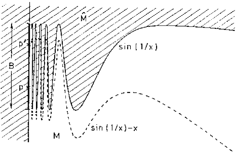
Figure 1: The manifold ${\cal M}$ lies below the curve $y=\sin(1/x)$ and to the right of the $y$-axis. Points of the boundary set $B$ are not the endpoints of any curves on ${\cal M}$.

Definition 14

If $B^{\prime}$ is a boundary set of a second envelopment $(\mbox{${\cal M}$},\mbox{$\widehat{\cal M}$}^{\prime},\phi^{\prime})$ of ${\cal M}$ then we say $B$ covers $B^{\prime}$ if for every open neighbourhood ${\cal U}$ of $B$ in $\widehat{\cal M}$ there exists an open neighbourhood $\mbox{${\cal U}$}^{\prime}$ of $B^{\prime}$ in $\mbox{$\widehat{\cal M}$}^{\prime}$ such that

$$\phi\circ\phi^{\prime-1}\left(\rule[-4.30554pt]{0.0pt}{12.91663pt}\,\mbox{${\cal U}$}^{\prime}\cap\,\phi^{\prime}({\mbox{${\cal M}$}})\,\right)\,\subset\,\mbox{${\cal U}$}\,.$$ (1)

The situation is as depicted in Figure 2. In effect condition (1) says that one cannot get close to points of $B^{\prime}$ by a sequence of points from within ${\cal M}$ without at the same time approaching some point of $B$ (see Theorem 19 for a more precise statement of this).

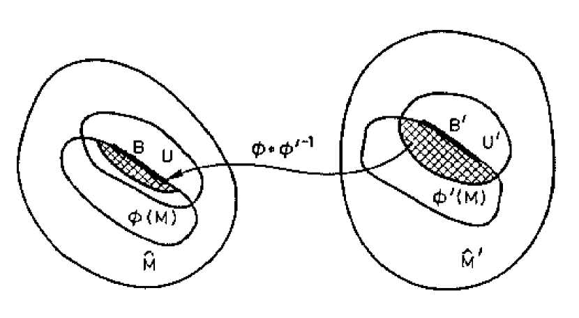
Figure 2: The set $B$ covers the set $B^{\prime}$.

If $p^{\prime}$ is a boundary point of the envelopment $(\mbox{${\cal M}$},\mbox{$\widehat{\cal M}$}^{\prime},\phi^{\prime})$ we shall say the boundary set $B$ covers (respectively is covered by) $p^{\prime}$ to mean $B$ covers (is covered by) the singleton boundary set $\{p^{\prime}\}$. Clearly if $p$ is a boundary point lying in the boundary set $B$ then $B$ covers $p$. It is also possible, however, for a single boundary point to cover a much larger boundary set, as the following example demonstrates.

Example 15

Let $\mbox{${\cal M}$}=\dot{\mathbb{R}}\raise 4.30554pt\hbox{$\scriptstyle n$}={\mathbb{R}}^{n}-\{O\}$ and $\phi=\mbox{id}:\mbox{${\cal M}$}\rightarrow{\mathbb{R}}^{n}$ be the trivial envelopment. Let $\phi^{\prime}:\mbox{${\cal M}$}\rightarrow{\mathbb{R}}^{n}$ be defined by

$$\phi^{\prime}(x_{1},\ldots,x_{n})=\frac{(r+1)}{r}\>(x_{1},\ldots,x_{n}),\mbox{ where }r=\sqrt{{\textstyle\sum_{i=1}^{n}}x_{i}^{2}}\>.$$

The origin $O$ is a boundary point of $\phi$ and covers the entire boundary set $S^{n-1}(O,1)$ [the unit sphere centre $O$] of $\phi^{\prime}$.

Theorem 16

A boundary set $B$ covers a boundary set $B^{\prime}$ if and only if it covers every boundary point $p^{\prime}\in B^{\prime}$.

Proof: The “only if” direction is trivial. To prove the “if” direction suppose $B$ covers every point $p^{\prime}\in B^{\prime}$. Let ${\cal U}$ be any open neighbourhood of $B$ in $\widehat{\cal M}$. For each $p^{\prime}\in B^{\prime}$ let $\mbox{${\cal U}$}^{\prime}_{p^{\prime}}$ be an open neighbourhood of $p^{\prime}$ in $\mbox{$\widehat{\cal M}$}^{\prime}$ such that $\phi\,\circ\phi^{\prime-1}(\mbox{${\cal U}$}^{\prime}_{p^{\prime}}\cap\phi^{\prime}(\mbox{${\cal M}$}))\subset\mbox{${\cal U}$}$. The set $\mbox{${\cal U}$}^{\prime}=\bigcup_{p^{\prime}\in B^{\prime}}\mbox{${\cal U}$}^{\prime}_{p^{\prime}}$ is clearly an open neighbourhood of $B^{\prime}$ in $\mbox{$\widehat{\cal M}$}^{\prime}$ satisfying (1), hence $B$ covers $B^{\prime}$.

 

It is commonly of great interest to compare the approach to two boundary sets along curves in the manifold ${\cal M}$. In this regard the following theorem is very useful.

Theorem 17

If a boundary set $B$ covers a boundary set $B^{\prime}$ then every curve $\gamma$ in ${\cal M}$ which approaches $B^{\prime}$ also approaches $B$.

Proof: Suppose $B$ covers $B^{\prime}$. Let $\gamma:[a,b)\rightarrow\mbox{${\cal M}$}$ be a curve which approaches $B^{\prime}$ and let $p^{\prime}\in B^{\prime}$ be a limit point of $\phi^{\prime}\circ\gamma$. Suppose $\gamma$ does not approach $B$. Let $t_{i}\rightarrow b$ be an increasing infinite sequence of real numbers such that $\phi^{\prime}\circ\gamma(t_{i})\rightarrow p^{\prime}$, and set $A=\{\phi\circ\gamma(t_{i});i\in{\mathbb{N}}\}$. Then $\mbox{${\cal U}$}=\mbox{$\widehat{\cal M}$}-\bar{A}$ is an open neighbourhood of $B$ and since $B$ covers $B^{\prime}$, there exists an open neighbourhood  $\mbox{${\cal U}$}^{\prime}$ of $B^{\prime}$ in $\mbox{$\widehat{\cal M}$}^{\prime}$ satisfying condition (1). As  $\mbox{${\cal U}$}^{\prime}$ is also an open neighbourhood of $p^{\prime}$ there exists an $n$ such that $\phi^{\prime}\circ\gamma(t_{i})\in\mbox{${\cal U}$}^{\prime}$ for all $i>n$. Clearly $\phi\,\circ\,\gamma(t_{i})=\phi\,\circ\,\phi^{\prime-1}\,\circ\,\phi^{\prime}\,\circ\,\gamma(t_{i})\in\mbox{${\cal U}$}$ for $i>n$, which contradicts $A\,\cap\>\mbox{${\cal U}$}\,=\,\mbox{\O}\,$. Hence $\gamma$ must have a limit point in $B$.

 

It is worth pointing out that the converse to this theorem definitely does not hold. For instance, in Example 13 let $p=(0,-1/2)$ and $p^{\prime}=(0,1/2)$. Any curve in ${\cal M}$ approaching $p^{\prime}$ must also approach $p$. $\{p\}$ does not cover $\{p^{\prime}\}$, however, since these two points clearly have non-intersecting open neighbourhoods ${\cal U}$ and $\mbox{${\cal U}$}^{\prime}$ and as $\phi=\phi^{\prime}=\mbox{id}\>$ in this example, condition (1) reduces to $\mbox{${\cal U}$}^{\prime}\cap\mbox{${\cal M}$}\subset\mbox{${\cal U}$}$ (see Figure 1). The following is probably the best that can be said in this respect.

Theorem 18

If every curve in ${\cal M}$ which approaches a boundary set $B^{\prime}$ also approaches a boundary set $B$, and if every neighbourhood of $B$ in $\widehat{\cal M}$ contains an open neighbourhood  ${\cal U}$ of $B$ whose complement in $\phi(\mbox{${\cal M}$})$ is connected, then $B$ covers $B^{\prime}$.

Proof: Suppose that all curves $\gamma$ in ${\cal M}$ which approach $B^{\prime}$ also approach $B$, but assume that $B$ does not cover $B^{\prime}$. Then by Theorem 16 there exists a $p^{\prime}\in B^{\prime}$ such that $B$ does not cover $p^{\prime}$. Hence there exists an open neighbourhood ${\cal U}$ of $B$ in $\widehat{\cal M}$ such that for every open neighbourhood $\mbox{${\cal U}$}^{\prime}$ of $p^{\prime}$ in $\mbox{$\widehat{\cal M}$}^{\prime}$ the set $\phi\circ\phi^{\prime-1}(\mbox{${\cal U}$}^{\prime}\cap\phi^{\prime}(\mbox{${\cal M}$}))$ contains points not belonging to ${\cal U}$. By our hypothesis there is no loss of generality in assuming $\phi(\mbox{${\cal M}$})-\mbox{${\cal U}$}$ to be a connected set. Now by paracompactness we can always make the manifold $\mbox{$\widehat{\cal M}$}^{\prime}$ into a metric space (e.g. by imposing a Riemannian metric on $\mbox{$\widehat{\cal M}$}^{\prime}$ and defining $d(x,y)$ to be the shortest distance for all curves connecting $x$ and $y$). Let $\mbox{${\cal U}$}^{\prime}_{n}=\{q^{\prime}\in\mbox{$\widehat{\cal M}$}^{\prime};d(p^{\prime},q^{\prime})<1/n\}$. For each $n$ select a point $p_{n}\in\phi\circ\phi^{\prime-1}(\mbox{${\cal U}$}^{\prime}_{n}\cap\phi^{\prime}(\mbox{${\cal M}$}))$ such that it does not lie in ${\cal U}$. Let $\gamma$ be a curve connecting $p_{1}$ to $p_{2}$ to $p_{3}$ to … and lying entirely in $\phi(\mbox{${\cal M}$})-\mbox{${\cal U}$}$. This curve can clearly be made $C^{1}$ and does not have any limit points in $B$. It certainly does have $p^{\prime}$ as a limit point, however, since $\phi^{\prime}\circ\phi^{-1}(p_{n})$ is a sequence of points approaching $p^{\prime}$. We therefore have a contradiction and $B$ must cover $B^{\prime}$.

 

Whilst Theorems 17 and 18 represent the best we can achieve in terms of approaches along parametrised curves in ${\cal M}$, a simpler result holds if one only requires approaches by sequences of points in ${\cal M}$. The following theorem is proved by methods essentially following those of Theorems 17 and 18. We therefore omit the proof.

Theorem 19

$B$ covers $B^{\prime}$ if and only if for every sequence $p_{1},p_{2},\ldots$ of points in ${\cal M}$ such that the sequence $\phi^{\prime}(p_{i})$ has a limit point in $B^{\prime}$, the sequence $\phi(p_{i})$ has a limit point in $B$.

Covering is a weak partial order on boundary sets:

1. $B$ covers $B$.

2. If $B$ covers $B^{\prime}$ and $B^{\prime}$ covers $B^{\prime\prime}$ then $B$ covers $B^{\prime\prime}$.

Definition 20

We say boundary sets $B$ and $B^{\prime}$ are equivalent if $B$ covers $B^{\prime}$ and $B^{\prime}$ covers $B$.

This is clearly an equivalence relation on the set of all boundary sets.

Definition 21

An abstract boundary set is an equivalence class of boundary sets, denoted $[B]$.

The covering relation passes to abstract boundary sets in the natural way; we say $[B]$ covers $[B^{\prime}]$ if and only if $B$ covers $B^{\prime}$. This relation is clearly independent of the choice of representatives. For abstract boundary sets, however, the covering relation is a true partial order as it satisfies the further antisymmetric condition:

$$\mbox{3. If }[B]\mbox{ covers }[B^{\prime}]\mbox{ and }[B^{\prime}]\mbox{ covers }[B]\mbox{ then }[B]=[B^{\prime}].$$

One might be tempted at this stage to define “abstract boundary points” as minimal abstract boundary sets, but any such attempt using an argument based on Zorn’s lemma is doomed to failure. Any single boundary point $p$ can always be blown up to a much larger boundary set in a similar way to Example 15. This is done by defining a new envelopment with the property that different curves in ${\cal M}$ which originally all had $p$ as their endpoints now approach separate endpoints (e.g., see [6]). Despite this problem we shall make the following definition of an abstract boundary point.

Definition 22

(The Abstract Boundary) For a manifold ${\cal M}$, an abstract boundary set is an abstract boundary point whenever it has a singleton $\{p\}$ as a representative boundary set. In this case the equivalence class is denoted by $[p]$. The set of all abstract boundary points will be denoted ${\cal B}(\cal M)$ and called the abstract boundary or a-boundary of ${\cal M}$.

It is to be stressed here that the abstract boundary is defined for every manifold ${\cal M}$, irrespective of the existence of further structure on the manifold such as a metric, affine connection or chosen family ${\cal C}$ of curves.

It must be realised, however, that an abstract boundary point $[p]$ is no more “pointlike” than a more general abstract boundary set $[B]$. The equivalence class $[p]$ need not even consist only of connected boundary sets. For example if one embeds the open interval $\mbox{${\cal M}$}=(0,1)$ in the natural way in the real line and then embeds it in the unit circle (using angular coordinate $\theta$) with the map $\theta=\phi(t)=2\pi t$, then clearly the single boundary point $\theta=0$ of the envelopment $(\mbox{${\cal M}$},S^{1},\phi)$ is equivalent to the disconnected boundary set $\{t=0,t=1\}$ of the first embedding.

It is not hard to show that every boundary set belonging to the equivalence class of an abstract boundary point $[p]$ must be a compact set, but whether this is a necessary and sufficient condition is difficult to resolve.

For the remainder of this section it will be assumed that a family ${\cal C}$ of curves with the b.p.p. has been chosen for the manifold ${\cal M}$ and this will be denoted by (${\cal M}$, ${\cal C}$).

Definition 23

If $(\mbox{${\cal M}$},\mbox{$\widehat{\cal M}$},\phi)$ is an envelopment of (${\cal M}$, ${\cal C}$) by $\widehat{\cal M}$, then we say a boundary point $p$ of this envelopment is a ${\cal C}$-boundary point or approachable if it is a limit point of some curve from the family ${\cal C}$ (in other words, if some curve of the family approaches $p$). Boundary points which are not ${\cal C}$-boundary points will be called unapproachable.

If a boundary point $p$ covers another boundary point $p^{\prime}$ and $p^{\prime}$ is a ${\cal C}$-boundary point, then it is clear by Theorem 17 that so is $p$, since any curve which approaches $p^{\prime}$ must also approach $p$. This leads naturally to the following definition.

Definition 24

An abstract boundary point $[p]$ is an abstract ${\cal C}$-boundary point, or simply approachable, if $p$ is a ${\cal C}$-boundary point. Similarly, an abstract boundary point $[p]$ is unapproachable if $p$ is not a ${\cal C}$-boundary point.

This definition is clearly independent of the choice of representative boundary point $p$. We denote the set of abstract ${\cal C}$-boundary points of ${\cal M}$ by ${\cal B}_{\cal C}(\mbox{${\cal M}$})$. Note how properties such as being approachable only have to be preserved one way under covering in order to pass to the abstract boundary. For example, the converse of the statement just prior to Definition 24 is certainly not true—${\cal C}$-boundary points may cover unapproachable boundary points, as the following example demonstrates.

Example 25

Consider the manifold $\mbox{${\cal M}$}=\{(x,y)\in{\mathbb{R}}^{2};\;-\infty<x<\infty,\;0<y<\infty\}$ with the metric d$s^{2}=y^{2}\,$d$x^{2}\>+\>$d$y^{2}$ (this is the covering space of the cone [4], or the Riemann surface of $\log(z)$). We set $\mbox{${\cal C}$}=\mbox{${\cal C}$}_{g}(\mbox{${\cal M}$})$, the family of affinely parametrised geodesics on ${\cal M}$. Let $\phi:\mbox{${\cal M}$}\rightarrow{\mathbb{R}}^{2}$ be the trivial envelopment defined by $\phi\,(x,y)=(x,y)$. Every boundary point on $y=0$ is a ${\cal C}$-boundary point, since it is the endpoint of a vertical geodesic $x=\mbox{constant}$. Furthermore, these are the only geodesics which approach the boundary $y=0$, since the general geodesic is given by $y=\alpha\sec(x-x_{0}),\alpha>0,\,|x-x_{0}|<\pi/2$ . A second envelopment $\phi^{\prime}:\mbox{${\cal M}$}\rightarrow{\mathbb{R}}^{2}$ defined by

$$(x^{\prime},y^{\prime})=\phi^{\prime}(x,y)=\left(\rule[-2.15277pt]{0.0pt}{17.22217pt}\,\frac{x}{y}\>,\sqrt{x^{2}+y^{2}}\;\right)$$

again maps ${\cal M}$ onto the region $y^{\prime}>0$ of  ${\mathbb{R}}^{2}$. It has the effect of spreading out the vertical geodesics $x=a\neq 0$ so that they approach $y^{\prime}=|a|$ as $x^{\prime}\rightarrow\pm\infty$. Thus on the boundary $y^{\prime}=0$ only the origin $(0,0)$ is a ${\cal C}$-boundary point, all others $(x^{\prime}\neq 0\,,y^{\prime}=0)$ being unapproachable. It is also easily seen that all these unapproachable boundary points are covered by the ${\cal C}$-boundary point $(0,0)$ of the original envelopment $\phi$.

4 Pseudo-Riemannian manifolds

Extensions

We now introduce a metric on ${\cal M}$. In order to establish conventions, we first give a standard definition.

Definition 26

A $C^{k}$ metric $g$ on ${\cal M}$ is a second rank covariant symmetric and non-degenerate $C^{k}$ tensor field on ${\cal M}$. The pair $(\mbox{${\cal M}$},g)$ is called a $C^{k}$ pseudo-Riemannian manifold. When $g$ is positive definite it is called Riemannian.

Our discussion will refer to metrics of any signature unless specifically stated otherwise. An envelopment of a pseudo-Riemannian manifold will be denoted $(\mbox{${\cal M}$},g,\mbox{$\widehat{\cal M}$},\phi)$. The metric ${({\phi^{-1}})^{*}}g$ induced on the open submanifold $\phi(\mbox{${\cal M}$})$ of $\widehat{\cal M}$ by the $C^{\infty}$ embedding $\phi$ will also be denoted by $g$ when there is no risk of ambiguity.

Definition 27

A $C^{l}$ extension $(1\leq l\leq k)$ of a $C^{k}$ pseudo-Riemannian manifold $(\mbox{${\cal M}$},g)$ is an envelopment of it by a $C^{l}$ pseudo-Riemannian manifold $(\mbox{$\widehat{\cal M}$},\hat{g})$ such that

$$\hat{g}|_{\phi({\cal M})}=g,$$

denoted $(\mbox{${\cal M}$},g,\mbox{$\widehat{\cal M}$},\hat{g},\phi)$. When $l=k$, we talk simply of $(\mbox{$\widehat{\cal M}$},\hat{g})$ being an extension of $(\mbox{${\cal M}$},g)$.

We note that this definition of an extension of a pseudo-Riemannian manifold $(\mbox{${\cal M}$},g)$ can be applied in a precisely analogous manner to a manifold ${\cal M}$ simply endowed with a $C^{k}$ affine connection $\nabla$, denoted $(\mbox{${\cal M}$},\nabla)$. Furthermore, this will also be true for all definitions to follow. It is important to keep this in mind, since it means that our scheme can be applied to a wide class of theories including conformal, projective and gauge theories.

Regular Boundary Points

Definition 28

We say a boundary point $p$ of an envelopment $(\mbox{${\cal M}$},g,\mbox{$\widehat{\cal M}$},\phi)$ is $C^{l}$ regular for $g$ if there exists a $C^{l}$ pseudo-Riemannian manifold $(\mbox{${\cal M}$}\kern-8.20007pt\rule[8.1805pt]{7.20001pt}{0.19919pt}\,,\bar{g})$ such that $\phi(\mbox{${\cal M}$})\cup\{p\}\subseteq\mbox{${\cal M}$}\kern-8.20007pt\rule[8.1805pt]{7.20001pt}{0.19919pt}\subseteq\mbox{$\widehat{\cal M}$}$ and $(\mbox{${\cal M}$},g,\mbox{${\cal M}$}\kern-8.20007pt\rule[8.1805pt]{7.20001pt}{0.19919pt}\,,\bar{g},\phi)$ is a $C^{l}$ extension of $(\mbox{${\cal M}$},g)$.

Note that we require the same mapping $\phi$ for the extension as for the original envelopment (although strictly speaking, since the target set ${\cal M}$  is different to the target set $\widehat{\cal M}$ of $\phi$, it should be given a new name $\bar{\phi}$ defined by the requirement that $\bar{\phi}(q)=\phi(q)$ for all $q\in\mbox{${\cal M}$}$).

A $C^{k}$ regular boundary point will simply be called regular. Although there is no serious loss of generality in using this term (since if $l<k$ we may simply regard $(\mbox{${\cal M}$},g)$ as being a $C^{l}$ pseudo-Riemannian manifold), we shall persist in our terminology because the distinction does become important for singular boundary points.

The notion of regularity cannot, however, be transferred to the abstract boundary as it stands, since it is not invariant under equivalence of boundary points. The following simple example clearly demonstrates this fact.

Example 29

Embed the one-dimensional manifold $\mbox{${\cal M}$}=(0,1)$ with metric d$s^{2}=\;$d$x^{2}$ into the manifold $\mathbb{R}$ in two ways: $y=\phi(x)=x$ and $z=\phi^{\prime}(x)=x^{1/2}$. The boundary points $y=0$ and $z=0$ are clearly equivalent by our earlier definitions, but the first is $C^{\infty}$ regular while the second is not $C^{l}$ regular for any $l\geq 1$. This follows because the metric induced by the second embedding,

$${\rm d}s^{2}=\,4z^{2}\,{\rm d}z^{2},$$

is degenerate at $z=0$ and cannot therefore be extended to any open interval $(-a,1)$, where $a>0$. Thus the abstract boundary point in question has at least two representative boundary points, one of which is regular while the other is not.

The notions of an extension of a pseudo-Riemannian manifold $(\mbox{${\cal M}$},g)$ and a regular boundary point of an envelopment $(\mbox{${\cal M}$},g,\mbox{$\widehat{\cal M}$},\phi)$ are both completely independent of whether or not a family ${\cal C}$ of curves with the b.p.p. has been chosen for ${\cal M}$. This will not be true for the notions which follow, such as a “point at infinity” and a “singular boundary point”. Therefore we shall henceforth always assume that our pseudo-Riemannian manifold is endowed with a family ${\cal C}$ of curves with the b.p.p. which normally (i.e. unless otherwise specified) includes the family of all geodesics with affine parameter $\mbox{${\cal C}$}_{g}(\mbox{${\cal M}$})$. The general situation will be denoted $(\mbox{${\cal M}$},g,\mbox{${\cal C}$})$ while the usual notation $(\mbox{${\cal M}$},g)$ will be reserved for the case where $\mbox{${\cal C}$}=\mbox{${\cal C}$}_{g}(\mbox{${\cal M}$})$. An envelopment of a pseudo-Riemannian manifold with a family of curves satisfying the b.p.p. will be denoted $(\mbox{${\cal M}$},g,\mbox{${\cal C}$},\mbox{$\widehat{\cal M}$},\phi)$.

The following example shows that regular boundary points can even be unapproachable by geodesics in ${\cal M}$.

Example 30

Let ${\cal M}$ be the open submanifold of  ${\mathbb{R}}^{2}$ defined by $y>x^{1/2},x>0$ and let $g$ be the usual flat metric d$s^{2}=\;$d$x^{2}\>+\>$d$y^{2}$. The boundary point $(0,0)$ is $C^{\infty}$ regular since the metric extends to all of ${\mathbb{R}}^{2}$, yet it is clearly unapproachable by any geodesics (straight lines) in ${\cal M}$.

Points at Infinity

The non-regular boundary points can be broken up into two groups, those which are ${\cal C}$-boundary points, also called approachable, and the rest which are unapproachable. Although we have seen examples of regular boundary points which are unapproachable (Example 30), the non-regular unapproachable boundary points do not seem to merit serious further discussion. This is because they usually occur when we blow up a region of a boundary by spreading out a family of approaching curves too thinly (e.g. Example 25).

The approachable non-regular boundary points do, however, have a very rich structure. First one must ask of them whether one can effectively ever “get there” along a curve in ${\cal C}$ with a finite value of the parameter or not. To this end we introduce the concept of a point at infinity.

Definition 31

Given an $(\mbox{${\cal M}$},g,\mbox{${\cal C}$})$ we will say that a boundary point $p$ of the envelopment $(\mbox{${\cal M}$},g,\mbox{${\cal C}$},\mbox{$\widehat{\cal M}$},\phi)$ is a $C^{l}$ point at infinity for ${\cal C}$ if

(i) $\;\;p$ is not a $C^{l}$ regular boundary point,
(ii) $\>p$ is a ${\cal C}$-boundary point, and
(iii) no curve of ${\cal C}$ approaches $p$ with bounded parameter.

Condition (iii) says that for no interval $I=[a,b<\infty)$ is there a curve $\gamma:I\rightarrow\mbox{${\cal M}$}$ in the family ${\cal C}$ and an increasing infinite sequence of real numbers $\{t_{i}\}$ in $I$ such that

$$\phi\,(\gamma(t_{i}))\longrightarrow p\>\mbox{ as }\>t_{i}\rightarrow b\,.$$

Clearly a $C^{l}$ point at infinity is also a $C^{l^{\prime}}$ point at infinity for all $l^{\prime}>l$. In particular, it is always a $C^{k}$ point at infinity and there is no real loss of generality in simply calling it a point at infinity.

Note that by the bounded parameter property, the concept of a point at infinity is independent of the choice of parametrisation on the curves from ${\cal C}$ which approach $p$. It is here that the importance of imposing the bounded parameter property on ${\cal C}$ becomes evident.

Condition (i) ensures that no boundary point is classified as both regular and a point at infinity. Without it, such boundary points do, in fact, occur as made clear by the following two examples.

Example 32

In Example 30 let ${\cal C}$ consist of all the geodesics in ${\cal M}$ supplemented with the curves $x(t)=1/t^{2}$, $y(t)=C/t$, $C>1,\,1\leq t<\infty$. The boundary point $(0,0)$ is still regular (nothing has changed as regards the metric) but it is “at infinity” for ${\cal C}$, since it is approachable only by curves with unbounded parameter.

This example is somewhat artificial, in that the added curves, and more particularly the choice of their parametrisation, seem to have nothing to do with the metric. A rather more subtle example is the following, in which there is a regular boundary point which is geodesically approachable, but only by geodesics with unbounded affine parameter.

Example 33

Let $\widehat{\cal M}$ be the unit torus, i.e. ${\mathbb{R}}^{2}/{\mathbb{Z}}^{2}$, with the usual flat metric d$s^{2}=\;$d$x^{2}\>+\>$d$y^{2}$. Let $\gamma$ be the geodesic in $\widehat{\cal M}$ generated by the line $x=t\,,\,y=t\sqrt{2}\>(t\geq 0)$ and let $p$ be the point $(\frac{1}{2},\frac{1}{2})$. On the central line $L=\{(x,1/2)\,;\,0\leq x<1\}$ choose points

$$p_{\pm i}\,=\left(\rule[-2.15277pt]{0.0pt}{17.22217pt}\,\frac{1}{2}\left(\rule[-2.15277pt]{0.0pt}{17.22217pt}1\pm\frac{1}{2^{i}}\,\right),\,\frac{1}{2}\,\right),\hskip 50.00008pti=1,2,3,\ldots$$

For each $i=\pm 1,\pm 2,\ldots$ let $L_{i}$ be the closed line segment of length 1/2 and slope $\sqrt{2}$ centred on the point $p_{i}$ and let $L_{0}$ be a similar line segment with centre $p$. Now define ${\cal M}$ as the open submanifold of $\widehat{\cal M}$ consisting of the complement in $\widehat{\cal M}$ of this infinite set of closed line segments,

$$\mbox{${\cal M}$}=\mbox{$\widehat{\cal M}$}-\bigcup_{i\in\mathbb{Z}}L_{i}$$

(see Figure 3). Clearly $p$ is a boundary point of the envelopment $(\mbox{${\cal M}$},\mbox{$\widehat{\cal M}$},\mbox{id}_{\cal M})$ and is $C^{\infty}$ regular. Now apart from its starting point at $(0,0)$, the geodesic $\gamma$ does not pass through any point $(x,y)$ where $x$ and $y$ are both rational and, in particular, it does not pass through any of the points $p_{i}$ or $p$ on $L$. It follows that $\gamma$ lies completely in ${\cal M}$. Furthermore, there is an increasing infinite sequence of positive numbers $t_{n}\rightarrow\infty$ such that $\gamma(t_{n})$ all lie on $\mbox{${\cal M}$}\,\cap\,L$ and such that $\gamma(t_{n})\rightarrow p$. Thus $\gamma$ approaches $p$ and does so with unbounded affine parameter. The same is true of every geodesic in $\widehat{\cal M}$ with slope $\sqrt{2}$ which does not pass through any of the points $p_{i}$ or $p$. Moreover these are the only geodesics in ${\cal M}$ which approach $p$. Thus $p$ is $C^{\infty}$ regular yet it is like a point at infinity with respect to geodesics in ${\cal M}$.

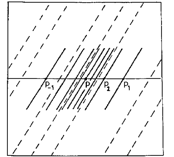
Figure 3: An example of a $C^{\infty}$ regular boundary point which is approachable only by geodesics in ${\cal M}$ with infinite affine parameter.

The key thing about these two examples is that regularity always takes precedence over being “at infinity”. Thus even if one can only “reach” the boundary point along curves from ${\cal C}$ having unbounded parameter, if it is regular then it will not be classified as a point at infinity. Suppose, however, that in Example 32 one were to perform a “bad” coordinate transformation, e.g., $x=x^{\prime 3},y=y^{\prime 3}$. If the manifold ${\cal M}$ is re-embedded in ${\mathbb{R}}^{2}$ with the new coordinates $x^{\prime},y^{\prime}$ taken as rectangular, then the origin definitely does become a point at infinity, since conditions (i), (ii) and (iii) of Definition 31 are now all satisfied. This point at infinity is, however, in a sense “artificial” or “removable”, since it is covered by (indeed equivalent to) the original regular boundary point at the origin. A similar bad transformation can be applied in a neighbourhood of the boundary point $(\frac{1}{2},\frac{1}{2})$ of Example 33, also converting it into a point at infinity.

Definition 34

We define a boundary point which is a point at infinity to be removable if it can be covered by a boundary set of another embedding consisting entirely of regular boundary points. When a point at infinity is not removable, it will be called essential.

In a sense essential points at infinity are boundary points which really do have a component at infinity (i.e., which cannot be transformed away). Furthermore the concept of being an essential point at infinity passes to the abstract boundary, as the following theorem demonstrates.

Theorem 35

If the boundary point $p$ is an essential point at infinity and $p$ is equivalent to the boundary point $p^{\prime}$, then $p^{\prime}$ is also an essential point at infinity.

Proof: Since $p^{\prime}$ covers $p$, it follows from Theorem 17 that it must be a ${\cal C}$-boundary point (since $p$ is a ${\cal C}$-boundary point). $p^{\prime}$ cannot be regular, else $p$ would be covered by a regular boundary point, contradicting it being an essential point at infinity. Now since $p$ also covers $p^{\prime}$, $p^{\prime}$ cannot be the limit point of any curve in ${\cal C}$ with bounded parameter else, by Theorem 17, $p$ would not be a point at infinity. Hence $p^{\prime}$ is a point at infinity. Furthermore it is an essential point at infinity for if $B$ is any boundary set of regular boundary points which covers $p^{\prime}$, then by transitivity of the covering relation this boundary set would also cover $p$, again contradicting its essentialness.

 

It is interesting to note that an essential point at infinity may itself cover regular boundary points. For example, if one is given an envelopment of a manifold which has both an unapproachable regular boundary point and an essential point at infinity, then it is in general a straightforward matter to create a new envelopment in which these two points are “joined together” to coalesce into a single new boundary point. This newly created boundary point would also be an essential point at infinity, but would cover the original regular boundary point.

Definition 36

An essential point at infinity which covers a regular boundary point will be called a mixed point at infinity. Otherwise it will be termed a pure point at infinity.

It is easy to see that both these categories are invariant under boundary point equivalence and therefore pass to the abstract boundary.

Singular Boundary Points

Definition 37

A boundary point $p$ of an envelopment $(\mbox{${\cal M}$},g,\mbox{${\cal C}$},\mbox{$\widehat{\cal M}$},\phi)$ will be called $C^{l}$ singular or a $C^{l}$ singularity if

(i) $\;\;p$ is not a $C^{l}$ regular boundary point,
(ii) $\>p$ is a ${\cal C}$-boundary point, and
(iii) there exists a curve from ${\cal C}$ which approaches $p$ with bounded parameter.

Alternatively, one could say $p$ is $C^{l}$ singular if it is a ${\cal C}$-boundary point which is not $C^{l}$ regular and not a $C^{l}$ point at infinity.

Since a boundary point which is not $C^{l}$ regular is clearly not $C^{l^{\prime}}$ regular for all $l^{\prime}\geq l$ it follows at once that if $p$ is $C^{l}$ singular then it is $C^{l^{\prime}}$ singular for all $l^{\prime}\geq l$—in particular, it is always $C^{k}$ singular. In general we shall simply say that $p$ is singular if it is $C^{k}$ singular (i.e., if $p$ is $C^{l}$ singular for some $l\leq k$).

Example 38

Consider the metric

$${\rm d}s^{2}=(1+r^{2n}){\rm d}r^{2}+r^{2}{\rm d}\theta^{2},\mbox{ where }r>0,\;0\leq\theta<2\pi$$

on the manifold $\mbox{${\cal M}$}=\,\dot{\mathbb{R}}\raise 4.30554pt\hbox{$\scriptstyle 2$}$ (see Example 15). This is the metric induced on the surface in ${\mathbb{E}}^{3}$ obtained by rotating the curve $z=r^{n+1}/(n+1)$ about the $z$-axis. The curvature scalar is readily shown to be proportional to $r^{2n-2}/(1+r^{2n})^{2}$ which $\rightarrow\infty$ as $r\rightarrow 0$ for $0<n<1$. In fact for $\frac{1}{2}<n<1$ one finds that the boundary point $r=0$ is $C^{1}$ regular but $C^{2}$ singular. Similarly for $N<2n<N+1$, where $n\in{\mathbb{N}}$, we have that $r=0$ is $C^{N}$ regular but $C^{N+1}$ singular. These results are easily seen by considering ${\cal M}$ as being embedded in ${\mathbb{R}}^{2}$ with the usual polar interpretation of the coordinates $(r,\theta)$ and then transforming to rectangular coordinates $(x,y)$.

Example 39

Consider the metric

$${\rm d}s^{2}={\rm d}r^{2}+(r+1)^{2}{\rm d}\theta^{2},\mbox{ where }0<r<\infty,\;0\leq\theta<2\pi$$

on the manifold $\mbox{${\cal M}$}=\,\dot{\mathbb{R}}\raise 4.30554pt\hbox{$\scriptstyle 2$}$. In this case the boundary point $r=0$ is singular if we use the natural polar embedding of ${\cal M}$ in ${\mathbb{R}}^{2}$. It is worth considering this example in some detail since at first sight the metric shows no pathological behaviour at the boundary point in question. The coordinates $(r,\theta)$ do not, however, constitute a coordinate patch for the manifold ${\mathbb{R}}^{2}$ in a neighbourhood of $r=0$. It is therefore necessary to perform a transformation to “rectangular” coordinates $\,x=r\cos\theta\,,\,y=r\sin\theta\,$, whereupon the metric becomes

$${\rm d}s^{2}=\,\frac{(r+1)^{2}}{r^{2}}\,({\rm d}x^{2}+{\rm d}y^{2})\,-\,\frac{2r+1}{r^{4}}\,(x{\rm d}x+y{\rm d}y)^{2}\,.$$

It is easy to see that $x=y=0$ is not a regular boundary point since each metric component becomes infinite for almost all directions of approach. It is clearly not a point at infinity since it is approached by geodesics with bounded parameter, hence it is a singularity. Let us now re-embed ${\cal M}$ in ${\mathbb{R}}^{2}$ using the $\phi^{\prime}$ of Example 15. Then $\phi^{\prime}(\mbox{${\cal M}$})$ is the region $r>1$ of ${\mathbb{R}}^{2}$ and again using polar coordinates on ${\mathbb{R}}^{2}$, the induced metric on $\phi^{\prime}(\mbox{${\cal M}$})$ becomes the standard flat metric d$s^{2}=\;$d$r^{2}+r^{2}$d$\theta^{2}$. This can, of course, be extended to all of ${\mathbb{R}}^{2}$ using rectangular coordinates $(x,y)$. Thus the original singular boundary point $r=0$ is equivalent to the boundary set $S^{1}(O,1)$ which is made up entirely of $C^{\infty}$ regular boundary points. Such a singularity will be termed “removable”. We begin to formalise the message of this example with the following definition.

Definition 40

A boundary set $B$ will be called $C^{l}$ non-singular if none of its points are $C^{l}$ singular, i.e., if they are all either $C^{l}$ regular, $C^{l}$ points at infinity or unapproachable boundary points. (N.B. As discussed above, the first and last categories are not mutually exclusive.)

As in Example 39 singular boundary points can arise which are equivalent to $C^{l}$ non-singular boundary sets. Such boundary points should not be classified as “truly” or “essentially” singular and will be called “removable singularities”. Other examples are the one-dimensional Example 29 above and the boundary points $(r=2m\,,t=\mbox{constant})$ of the Schwarzschild “singularity”, which are all covered by the $C^{\infty}$ regular boundary point $(u=0,v=0)$ of the Kruskal–Szekeres extension [11, 19]. A more precise definition of this concept is now given.

Definition 41

A $C^{m}$ singular boundary point $p$ will be called $C^{m}$ removable if it can be covered by a $C^{m}$ non-singular boundary set $B$. Clearly if $p$ is a $C^{m}$ removable singularity, then for all $m^{\prime}\leq m$ such that $p$ is $C^{m^{\prime}}$ singular, it is also $C^{m^{\prime}}$ removable. If $m=k$ we say simply that $p$ is a removable singularity.

Definition 42

A $C^{m}$ singular boundary point $p$ will be called $C^{m}$ essential if it is not $C^{m}$ removable. If $p$ is $C^{m}$ essential then it is $C^{m^{\prime}}$ essential for all $m^{\prime}\geq m$, whence it is always $C^{k}$ essential and we can describe $p$ simply as an essential singularity.

Keeping track of all these orders of differentiability is a tedious business and from now on we will simply use the terms regular, singular, removable, essential, etc. in most cases. It is usually a straightforward matter to discover corresponding statements for more general orders of differentiability than $k$. It is worthwhile keeping in mind the following easily proved theorem, stating in essence that singularities can never be removed “to infinity”.

Theorem 43

Let $p$ be a removable singularity and let $B$ be any non-singular boundary set which covers $p$. Then $B$ contains at least one regular boundary point.

Proof: By Definition 37, there is a curve $\gamma$ from ${\cal C}$ which approaches $p$ with bounded parameter. Since $B$ covers $p$, $\gamma$ must also approach $B$ (by Theorem 17). Let $q\in B$ be any limit point of the curve $\gamma$. $q$ is clearly a ${\cal C}$-boundary point and since the curve $\gamma$ approaches it with bounded parameter, it is not a point at infinity. Hence $q$ must be a regular boundary point.

 

It is useful to further subclassify essential singularities and to this end we provide the following definition.

Definition 44

An essential singularity $p$ will be called a mixed or directional singularity if $p$ covers a boundary point $q$ which is either regular or a point at infinity. Otherwise, when $p$ covers no such boundary point, we shall call it a pure singularity.

These notions seem to encapsulate earlier discussions of “directional singularities” as they appear in the literature, particularly with regard to the Curzon solution [18, 5, 3]. Possibly the word “mixed” is better to use in this context since such a singularity might only cover an unapproachable regular boundary point, which would hardly make the behaviour dependent on the “direction of approach”. Nevertheless we will persevere with the more standard terminology and usually call such singularities directional.

Example 45

Consider the metric

$${\rm d}s^{2}=F^{2}(r)\,({\rm d}r^{2}+r^{2}{\rm d}\theta^{2}),\mbox{ where }r>0,\;0\leq\theta<2\pi\ \mbox{and }F^{2}(r)=1+r^{n}$$

defined on the two-dimensional manifold $\mbox{${\cal M}$}=\,\dot{\mathbb{R}}\raise 4.30554pt\hbox{$\scriptstyle 2$}$. When $0<n<2$ it is seen that the curvature scalar

$$R_{\mbox{\scriptsize curv}}=-\>\frac{n^{2}r^{n-2}}{(1+r^{n})^{3}}\,\rightarrow-\,\infty\>\mbox{ as }\>r\rightarrow 0\,,$$

so that the boundary point $r=0$ of the natural embedding of ${\cal M}$ in ${\mathbb{R}}^{2}$ is a $C^{2}$ singularity (it is clearly not a point at infinity). Now transform to elliptical coordinates $(\eta,\psi)$ given by

$$\begin{array}[]{ccccc}x&=&r\cos\theta&=&\cosh\eta\cos\psi\>,\\ y&=&r\sin\theta&=&\sinh\eta\sin\psi\>.\end{array}$$

In these coordinates the metric becomes

$${\rm d}s^{2}=F^{2}(r)\,({\rm cosh}^{2}\eta-{\rm cos}^{2}\psi)\,({\rm d}\eta^{2}+{\rm d}\psi^{2})\hskip 14.45377pt(0<\eta<\infty,\;0\leq\psi<2\pi)$$

where

$$r^{2}=\cosh^{2}\!\eta-\sin^{2}\!\psi\>.$$

In the $x-y$ plane, $\eta=0$ corresponds to the strip $-1\leq x\leq 1$ of the $x$-axis. If we now perform a transformation to “rectangular” coordinates $(X,Y)$ based on $(\eta,\psi)$ as “polars”, viz.,

$$X=\eta\cos\psi\>,\mbox{ }Y=\eta\sin\psi\>,$$

the metric assumes the rather prohibitive form

$${\rm d}s^{2}=\frac{F^{2}(r)}{\eta^{4}}\>\left(\rule[-2.15277pt]{0.0pt}{17.22217pt}\cosh^{2}\!\eta-\frac{X^{2}}{\eta^{2}}\,\right)\>[\>(\eta^{2}X^{2}+Y^{2})\,{\rm d}X^{2}+(\eta^{2}Y^{2}+X^{2})\,{\rm d}Y^{2}$$

$$\;\;\;\;\;\;\;+2XY(\eta^{2}-1)\,{\rm d}X{\rm d}Y\>]\>,$$

where

$$r^{2}=\cosh^{2}\!\eta-\frac{Y^{2}}{\eta^{2}}\>,\hskip 30.00005pt\eta=\sqrt{X^{2}+Y^{2}}\>.$$

Now suppose that we are presented with this metric in $(X,Y)$ coordinates, but without any words of explanation as to its origin. Taking $(X,Y)$ as rectangular coordinates on the manifold ${\mathbb{R}}^{2}$, we wish to classify the boundary point $(0,0)$ of $\,\dot{\mathbb{R}}\raise 4.30554pt\hbox{$\scriptstyle 2$}$. From evaluation of the curvature scalar, which must come to the same along a given curve as in the first embedding, one sees that $R_{\mbox{\scriptsize curv}}\rightarrow-\,\infty$ as one approaches the origin $X=Y=0$ ($\eta=0$) along the $Y-$axis. For any other direction of approach $X=\alpha Y$ ($\alpha\neq 0$), however, $R_{\mbox{\scriptsize curv}}$ can be shown to have a finite limit (see Figure 4). Typically this is the cue for a directional singularity. The way our example has been constructed it is a straightforward matter to see how the directionality may be unravelled. The boundary point $X=Y=0$ is equivalent to the strip $-1\leq x\leq 1$ of the $x-$axis $(\eta=0)$ in the original embedding, which consists of both a $C^{2}$ essentially singular boundary point and infinitely many $C^{2}$ regular boundary points. It follows that the origin of the second embedding is a $C^{2}$ directional singularity.

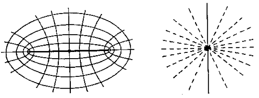
Figure 4: A directional singularity. A curvature singularity exists at the origin of the $(x,y)$ coordinate system on the left. The origin on the right induced by the use of elliptical coordinates is a directional singularity, as it covers the whole line segment $[-1,1]$ of the original $x-$axis, which consists of both a singular boundary point and infinitely many regular boundary points.

The following theorem implies that the property of being an essential singularity passes to the abstract boundary.

Theorem 46

If a boundary point $p$ of an envelopment $(\mbox{${\cal M}$},g,\mbox{${\cal C}$},\mbox{$\widehat{\cal M}$},\phi)$ covers a boundary point $p^{\prime}$ of a second envelopment $(\mbox{${\cal M}$},g,\mbox{${\cal C}$},\mbox{$\widehat{\cal M}$}^{\prime},\phi^{\prime})$ which is essentially singular, then $p$ is also an essential singularity.

Proof: The boundary point $p$ is a ${\cal C}$-boundary point since it covers the ${\cal C}$-boundary point $p^{\prime}$. It is neither regular nor a point at infinity, else $p^{\prime}$ would be covered by the non-singular boundary set $\{p\}$ and hence would be removable (i.e. not essential). Furthermore it must be an essential singularity, for if it were covered by a non-singular boundary set $B$, then $B$ would also cover $p^{\prime}$ by the transitivity of the covering relation, again contradicting the assumption that $p^{\prime}$ is an essential singularity.

 

5 Classification of boundary points

Suppose that we are given an envelopment $(\mbox{${\cal M}$},g,\mbox{${\cal C}$},\mbox{$\widehat{\cal M}$},\phi)$ of a $C^{k}$ pseudo-Riemannian manifold $(\mbox{${\cal M}$},g,\mbox{${\cal C}$})$ and wish to classify a specific boundary point $p$. We proceed by asking a series of questions. Each question is in principle decidable, though we do not mean to imply by this that the decision is always easy to carry out. The questions to be decided are:
(1) Is $p$ a $C^{l}$ regular boundary point for some $l\leq k$? This is usually a fairly straightforward thing to decide. If $p$ is regular then there must exist an open coordinate neighbourhood ${\cal U}$ of $p$ in $\widehat{\cal M}$ and a metric which extends $g$ in a $C^{l}$ manner from its restriction to $\,\mbox{${\cal U}$}\,\cap\,\mbox{${\cal M}$}$ to all of ${\cal U}$. If the answer is YES, we are finished, except for possibly enquiring whether $p$ is approachable (i.e. a ${\cal C}$-boundary point) or not. This latter question is again answerable by investigating whether $p$ is a limit point of some curve from ${\cal C}$.

For convenience, let us assume from now on that $l=k$ (corresponding questions to be decided for different orders of differentiability are easily posed). If the answer to question (1) is NO, then we must proceed as follows:
(2) Is $p$ a ${\cal C}$-boundary point? If NO, then $p$ is filed away as an unapproachable non-regular boundary point. These are essentially uninteresting points, though a further investigation might be carried out to ascertain whether they cover any (unapproachable) regular boundary points. If YES, then we proceed with the following questions:
(3) Is there a curve from ${\cal C}$ which approaches $p$ with bounded parameter? If NO, then $p$ is a point at infinity, while if YES, then it is a singularity.
If $p$ is a point at infinity we ask:
(4) Is $p$ covered by a boundary set $B$ of another embedding consisting only of regular and/or unapproachable boundary points? If YES, then the point at infinity is called removable, while if NO, then it is called essential. In the latter case we proceed to ask:
(5) Does $p$ cover a regular boundary point $q$ of another embedding? If YES, then $p$ is a mixed point at infinity, while if NO, then it is a pure point at infinity.
If $p$ is singular we ask:
(6) Is $p$ covered by a non-singular boundary set $B$ of another embedding? If YES, then it is a removable singularity, while if NO, then it is an essential singularity and we can ask further:
(7) Does $p$ cover any regular boundary points or points at infinity of other embeddings? If YES, then it is a directional singularity, while if NO, then it is a pure singularity.

The whole classification as it emerges from this sequence of questions is displayed schematically in Figure 5. Boxes surround concepts which pass to the abstract boundary.

Figure 5: Schematic classification of boundary points. Boxes surround concepts which are invariant under boundary point equivalence and therefore pass to the abstract boundary.

Covering Relations

There are eight principal categories of boundary points. These are the regular boundary points (approachable and unapproachable regular boundary points being regarded as subcategories); non-regular unapproachable boundary points; removable, mixed and pure points at infinity; removable, directional (mixed) and pure singularities. It is of interest to know which of these categories can or cannot cover each other. In Table 1 we put a $\surd$ if a boundary point of type corresponding to the row label can cover a boundary point of the type belonging to the column label (i.e., if an explicit example of such a covering can be found), while we put a $\times$ there if it is impossible. Most of the positions in the table are easy to fill in, although specific examples of a covering where it is possible can be a little tricky to find in some cases.

The value of the table is that it allows us to see at once which pairs of categories can or cannot have representatives which are equivalent to each other. This is particularly valuable when it comes to analysing the abstract boundary.

	reg	non-reg	rem	mix	pure	rem	dir	pure
		unapp	$\infty$	$\infty$	$\infty$	sing	sing	sing
regular	$\surd$	$\surd$	$\surd$	$\times$	$\times$	$\surd$	$\times$	$\times$
non-reg. unapp.	$\surd$	$\surd$	$\times$	$\times$	$\times$	$\times$	$\times$	$\times$
remov. pt. $\infty$	$\surd$	$\surd$	$\surd$	$\times$	$\times$	$\times$	$\times$	$\times$
mixed pt. $\infty$	$\surd$	$\surd$	$\surd$	$\surd$	$\surd$	$\times$	$\times$	$\times$
pure pt. $\infty$	$\times$	$\surd$	$\surd$	$\times$	$\surd$	$\times$	$\times$	$\times$
remov. sing.	$\surd$	$\surd$	$\surd$	$\surd$	$\surd$	$\surd$	$\times$	$\times$
dir. sing.	$\surd$	$\surd$	$\surd$	$\surd$	$\surd$	$\surd$	$\surd$	$\surd$
pure sing.	$\times$	$\surd$	$\times$	$\times$	$\times$	$\surd$	$\times$	$\surd$

Table 1: Covering table. A $\surd$ means that a row-labelled boundary point can cover a column-labelled one, $\times$ means this is impossible. The various labels are abbreviations for regular; non-regular unapproachable; removable, mixed and pure points at infinity; removable, directional and pure singularities.

Classification of the Abstract Boundary

We are now in a position to completely classify the abstract boundary points. First of all abstract boundary points can be divided into approachable (${\cal C}$-boundary points) and unapproachable. We essentially discard the latter, although there is an interesting subclass of unapproachable abstract boundary points which have a regular boundary point representative (Example 30). Focussing attention on approachable boundary points, we have already seen that the classes which belong to the essential categories, namely mixed and pure points at infinity and directional and pure singularities, all pass to the abstract boundary. To see that these are the only categories which pass to the abstract boundary one makes use of Table 1.

A category $C$ passes to the abstract boundary if and only if representative boundary points from $C$ can never be equivalent to points from another category $C^{\prime}$. This will be true if there is a $\times$ in either the $CC^{\prime}$ or $C^{\prime}C$ entry of the table for every category $C^{\prime}\neq C$. It is easily verified that the only categories for which this holds are those mentioned above. The remainder we may simply term “indeterminate”—these comprise abstract boundary points which have as members regular boundary points, removable points at infinity and removable singularities. As a regular boundary point can be equivalent either to a removable point at infinity or to a removable singularity (but never to both) it is not possible to create genuine subcategories of the indeterminate abstract boundary points. In view of all this it is reasonable to make the following definitions.

Definition 47

An abstract boundary point will be termed an abstract point at infinity if it has a representative boundary point which is an essential point at infinity.

Definition 48

An abstract boundary point will be termed an abstract singularity if it has a representative boundary point which is an essential singularity.

This classification together with the further subclassification into mixed (directional) and pure classes is depicted in Figure 6. In this way we see that every pseudo-Riemannian manifold with a class ${\cal C}$ of curves satisfying the b.p.p. has a well-defined abstract singular boundary (consisting of the set of all abstract singularities) and also an abstract infinity. This essentially solves the problem originally posed by this paper, namely to construct a boundary for an arbitrary $n$-dimensional pseudo-Riemannian manifold with class ${\cal C}$ of curves satisfying the b.p.p. which represents its singularities. The abstract infinity, representing the “boundary at infinity”, comes as a bonus.

Figure 6: Classification scheme for abstract boundary points.

6 Singularities of pseudo-Riemannian manifolds

Definition 49

We will say that a pseudo-Riemannian manifold $(\mbox{${\cal M}$},g,\mbox{${\cal C}$})$ with class ${\cal C}$ of curves satisfying the b.p.p. has a $C^{l}$ singularity if its abstract $C^{l}$ singular boundary is non-empty, i.e., if there exists an envelopment of ${\cal M}$ having an essentially $C^{l}$ singular boundary point. Conversely, $(\mbox{${\cal M}$},g,\mbox{${\cal C}$})$ will be called $C^{l}$ singularity-free if it has no $C^{l}$ singularities, i.e., if for every envelopment of ${\cal M}$ its boundary points are either $C^{l}$ non-singular ($C^{l}$ regular boundary points, $C^{l}$ points at infinity or unapproachable boundary points) or $C^{l}$ removable singularities.

At first sight it might seem a daunting prospect to decide whether a given $(\mbox{${\cal M}$},g,\mbox{${\cal C}$})$ is singularity-free, as it seems that one would have to investigate every possible envelopment of ${\cal M}$ and check whether it has any essential singularities or not. In practice, however, several very general theorems exist to make the task much simpler. The two which follow are generally regarded as the sine qua non of any successful theory of singularities [17].

Theorem 50

Every compact pseudo-Riemannian manifold $(\mbox{${\cal M}$},g)$ is singularity-free for any family ${\cal C}$ of curves with the b.p.p.

Proof: A compact manifold has no non-trivial envelopments, for any enveloping manifold $\widehat{\cal M}$ would contain ${\cal M}$ as a compact open subset. But ${\cal M}$ cannot be both open and closed, since the enveloping manifold $\widehat{\cal M}$ is assumed to be connected. Since ${\cal M}$ has no envelopments, its abstract boundary is empty and, in particular, can contain no singularities.

 

Theorem 51

Every pseudo-Riemannian manifold with a family ${\cal C}$ of curves satisfying the b.p.p., $(\mbox{${\cal M}$},g,\mbox{${\cal C}$})$, which is ${\cal C}$-complete is singularity-free.

Proof: Let $(\mbox{${\cal M}$},g,\mbox{${\cal C}$},\mbox{$\widehat{\cal M}$},\phi)$ be any envelopment of $(\mbox{${\cal M}$},g,\mbox{${\cal C}$})$ and let $p$ be any ${\cal C}$-boundary point of this envelopment. Let $\gamma:[a,b)\rightarrow\mbox{${\cal M}$}$ be some curve from ${\cal C}$ having $p$ as a limit point. The parameter range $[a,b)$ cannot be bounded, else by ${\cal C}$-completeness $\gamma$ would have an endpoint $q\in\mbox{${\cal M}$}$. Since endpoints are unique limit points and $q\neq p$ (since $p\not\in\mbox{${\cal M}$}$), it is clear that this yields a contradiction. Hence $p$ cannot be a singularity.

 

A rather stronger version of this theorem is available when, as is usually required, $\mbox{${\cal C}$}\supseteq\mbox{${\cal C}$}_{g}(\mbox{${\cal M}$})$. It implies that not even unapproachable regular boundary points are possible in this case, which would still have been permitted by Theorem 51.

Theorem 52

If the pseudo-Riemannian manifold $(\mbox{${\cal M}$},g)$ is $\mbox{${\cal C}$}_{g}(\mbox{${\cal M}$})$-complete then it can have no regular boundary points.

Proof: Let $(\mbox{${\cal M}$},g,\mbox{$\widehat{\cal M}$},\phi)$ be any envelopment of $(\mbox{${\cal M}$},g)$ and let $p$ be any boundary point of this envelopment. If $p$ is a regular boundary point then it is possible to find a neighbourhood ${\cal U}$ of $p$ in $\widehat{\cal M}$ on which a metric $\bar{g}$ exists which extends $g|_{{\cal U}\cap{\cal M}}$. There is no loss of generality in assuming that ${\cal U}$ is a normal neighbourhood. Let $q\in\mbox{${\cal U}$}\cap\mbox{${\cal M}$}$ and $\gamma:[a,b]\rightarrow\mbox{${\cal U}$}$ be the unique geodesic for the metric $\bar{g}$ connecting $q$ to $p$. This geodesic clearly intersects ${\cal M}$ (since $q\in\mbox{${\cal M}$}$) and has bounded parameter. On the other hand it must exit ${\cal M}$ since $p\not\in\mbox{${\cal M}$}$. Let the first parameter value $t\in(a,b]$ for which $\gamma(t)\not\in\mbox{${\cal M}$}$ be denoted by $c$. Clearly the geodesic $\gamma|_{[a,c)}$ does not have its endpoint $\gamma(c)$ in ${\cal M}$. This contradicts $\mbox{${\cal C}$}_{g}(\mbox{${\cal M}$})$-completeness, whence $p$ cannot be regular.

 

Of course it is possible for a pseudo-Riemannian manifold $(\mbox{${\cal M}$},g)$ to be $\mbox{${\cal C}$}_{g}(\mbox{${\cal M}$})$-complete and therefore to be singularity-free, but if the family of curves is extended to a wider class such as $\mbox{${\cal C}$}=\mbox{${\cal C}$}_{gap}(\mbox{${\cal M}$})$, it might no longer be ${\cal C}$-complete. A classic example of this kind has been given by Geroch [7], where a space–time is geodesically complete but has incomplete curves of bounded acceleration.

Definition 53

Boundary points arising as limit points of curves from the family ${\cal C}$ with bounded parameter in a $\mbox{${\cal C}$}_{g}(\mbox{${\cal M}$})$-complete manifold will be referred to as Geroch points.

Geroch points must be singular (as is clear from Theorem 52). In fact they must be essentially singular, else they would be covered by a boundary set of another embedding which contains at least one regular boundary point (by Theorem 43), which is impossible by Theorem 52. Thus the existence of Geroch points implies that the pseudo-Riemannian manifold $(\mbox{${\cal M}$},g,\mbox{${\cal C}$})$ has a singularity. Note, however, that if $\mbox{${\cal C}$}_{g}(\mbox{${\cal M}$})$-completeness had been taken as one’s goal, then the manifold would be singularity-free. It is therefore of vital importance to specify the family ${\cal C}$ of curves when discussing the question of singularities.

Also with this scheme, geodesic incompleteness does not necessarily imply that the particular $(\mbox{${\cal M}$},g,\mbox{${\cal C}$})$ in question has a singularity. The classic example of this is the Taub–NUT space–time [9] or Misner’s simplified version [12], which we present here.

Example 54

Let ${\cal M}$ be the 2-dimensional manifold $S^{1}\times{\mathbb{R}}^{1}$, with Lorentzian metric

$${\rm d}s^{2}=\,2\,{\rm d}t\,{\rm d}\psi+t\,{\rm d}\psi^{2},\mbox{ where }\>t\in{\mathbb{R}},\>0\leq\psi<2\pi\,.$$

The central circle $t=0$ and the vertical lines $\psi=$ constant are complete null geodesics, but there are other geodesics (null, timelike and spacelike) which execute infinite spirals as they approach $t=0$ from either above or below (see Figure 7). These geodesics all approach $t=0$ with bounded affine parameter and thus are either past- or future-incomplete. On the other hand it is clear that there is no envelopment of this space–time providing boundary points which are limit points of these incomplete curves (this is seen most readily by compactifying the space into a torus by identifying $t=-\infty$ with $t=+\infty$, for then no envelopments exist at all, as was shown in Theorem 50). Hence this space–time is singularity-free but is geodesically incomplete. In many sources [17, 4] this space–time is classified as singular. This interpretation seems to arise in part because more than one extension is possible across $t=0$. Thus an extension of the lower half-space ($t<0$) exists in which the spiralling geodesics are complete, but the vertical ones become incomplete spirals. Undesirable as this sort of behaviour may be physically, we do not see it as grounds for calling the space–time singular. Indeed, there can be other reasons apart from singularities for discarding a metric on physical grounds—for example, the existence of closed causal curves. These, incidentally, are also present in the Misner space–time.

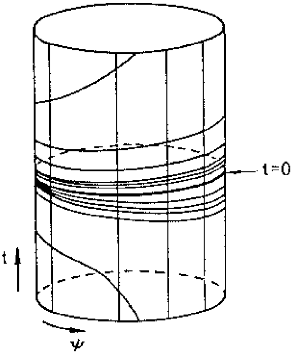
Figure 7: Misner’s example.

7 Conclusions

We have presented a new definition of singularities which can be applied equally well to manifolds of any dimension and metric of any signature. The key idea has been to define the abstract boundary or a-boundary ${\cal B}(\cal M)$ of a manifold ${\cal M}$. This is definable for any manifold whatsoever and includes, in a sense, all possible boundary points which can arise from open embeddings of the manifold. The a-boundary is constructed entirely from the manifold itself and is therefore something which every manifold gets gratis. When the manifold is endowed with extra structure, such as a pseudo-Riemannian metric or an affine connection, then the approachable boundary points can be classified into three important categories—regular boundary points, points at infinity and singularities, together with further subcategories. The key to this classification is the specification of a family of parametrised curves in the manifold satisfying the bounded parameter property. This is a vital ingredient, for different such families will give rise to different singularity structures. It is usual, however, to insist that the family does include all affinely parametrised geodesics.

The scheme presented is, we believe, very robust and passes most standard tests required of a theory of singularities. Furthermore, it is a practical scheme, for when a pseudo-Riemannian manifold such as a space–time is presented, it is usually given in a specific coordinate system. This often amounts to giving an envelopment of the manifold in question. It is normally then a relatively straightforward matter to classify the boundary points (and, by equivalence, the abstract boundary points of which they are representatives) arising from this envelopment. Frequently the information so obtained is sufficient to obtain an analysis of the a-boundary which at least suffices for answering the main questions about the singularity structure of the particular pseudo-Riemannian manifold. Some examples can be found in ref. [14] and others will be given in a forthcoming paper.

One of the great benefits of our scheme is that when a closed region is excised from a singularity-free pseudo-Riemannian manifold, the resulting pseudo-Riemannian manifold is still singularity-free, since only regular boundary points are introduced by the excision process. It was never possible to make such a claim with previous schemes because geodesics always had to be maximally extended before the discussion could begin. As maximal extensions of pseudo-Riemannian manifolds are not easy to find and are not even unique in the analytic case, we believe this to be a great advantage of our approach.

Finally, a number of questions remain unanswered in this paper. In particular, no mention has been made of the topology of the a-boundary, especially its singular part. This is an important topic, which we propose to discuss in another paper. It would be of great interest to know how the a-boundary and its topology relates to the Cauchy completion in the case of a Riemannian manifold. Another interesting question is the following: does every essential singularity cover a pure singularity? In other words, is there always a “pure core” to the singular part of the a-boundary? For any envelopment of a pseudo-Riemannian manifold, is every boundary point coverable by a boundary set of some embedding, all of whose boundary points are approachable by geodesics? Does every manifold ${\cal M}$ have an envelopment such that its closure ${\cal M}$  is compact, i.e., does ${\cal M}$ have a compactification? Obviously one could go on, but despite the interest of such questions there is nothing in them to negate the consistency and completeness of our scheme.

A question of particular interest would be to see how the a-boundary relates to other boundary constructions such as the b-boundary or g-boundary. As it stands it is difficult to see any connection, at least until the further topic of topology on the boundary is addressed. Our main objective in this paper has been to answer the question when is a manifold with affine connection and preferred family of curves singular? The a-boundary seems to be a satisfactory vehicle for dealing with this question. The criteria we have arrived at are unambiguous and in many cases can be readily shown to give the expected answer (see ref. [14] for applications to such examples as Schwarzschild, Friedmann, Curzon, etc.). To explicitly display the a-boundary of a given manifold, however, is not a feasible proposition in general, since it amounts to specifying every inequivalent way in which the manifold can be embedded as an open submanifold of a larger manifold. Because of the prevalence of “blow-up” maps, this is clearly not a practical thing to do. Some method for cutting down or “sectioning” the a-boundary into manageable sized portions will be needed before structures such as topology can be attached. We will present procedures for doing this in a forthcoming publication.

Acknowledgements

P.S. would like to express his appreciation to the Department of Applied Mathematics, University of Waterloo and particularly to R.G. McLenaghan for their hospitality during some of this work. S.M.S. would like to express her appreciation to the Aspen Center for Physics, Colorado, where some of this work was also carried out. We have benefitted greatly from discussions with C.J.S. Clarke, R. Geroch, R. Penrose, W. Unruh and J. Vickers. We would also like to thank the referee B.G. Schmidt for some helpful suggestions regarding the readability of the paper, as well as members of the Mathematical Relativity Group at the Australian National University for carefully checking the manuscript.

References

- [1] B. Bosshard, On the -boundary of the closed Friedman-model, Comm. Math. Phys. 46 (1976) 263–268.
- [2] C.J.S. Clarke and B.G. Schmidt, Singularities: the state of the art, Gen. Rel. and Grav. 8 (1972) 129–137.
- [3] F.I. Cooperstock, G.J.G. Junevicus and A.R. Wilson, Critique of the directional singularity concept, Physics Letters 42A (1972) 203–204.
- [4] G.F.R. Ellis and B.G. Schmidt, Singular space–times, Gen. Rel. and Gravitation 8 (1977) 915–953.
- [5] R. Gautreau, On equipotential areas and directional singularities, Physics Letters 28A (1969) 606–607.
- [6] R.P. Geroch, Local characterization of singularities in general relativity, J. Math. Phys. 9 (1968) 450–465.
- [7] R.P. Geroch, What is a singularity in general relativity, Ann. Phys. (N.Y.) 48 (1968) 526–540.
- [8] R.P. Geroch, E.H. Kronheimer and R. Penrose, Ideal points in space–time, Proc. Roy. Soc. A 327 (1972) 545–567.
- [9] S.W. Hawking and G.F.R. Ellis, The Large Scale Structure of Space–Time (Cambridge University Press, 1973).
- [10] S. Helgason, Differential Geometry and Symmetric Spaces (Princeton University Press, 1965).
- [11] M.D. Kruskal, Maximal extensions of Schwarzschild metric, Phys. Rev. 119 (1960) 1743–1745.
- [12] C.W. Misner, Taub–NUT spaces as a counterexample to almost anything, Relativity Theory and Astrophysics I: Relativity and Cosmology, ed. J. Ehlers, Lectures in Applied Mathematics, Vol. 8 (AMS, 1967) 160–169.
- [13] B.G. Schmidt, A new definition of singular points in general relativity, Gen. Rel. and Grav. 1 (1971) 269–280.
- [14] S.M. Scott, in Relativity Today, edited by Z. Perjés (Nova Science Publishers, New York 1992) 165–194.
- [15] S.M. Scott and P. Szekeres, The Curzon singularity I: spatial sections, Gen. Rel. and Gravitation 18 (1986) 557–570.
- [16] S.M. Scott and P. Szekeres, The Curzon singularity II: global picture, Gen. Rel. and Gravitation 18 (1986) 571–583.
- [17] L. Shepley and G. Ryan, Homogeneous Cosmological Models (Princeton University Press, 1978).
- [18] J. Stachel, Structure of the Curzon metric, Physics Letters 27A (1968) 60–61.
- [19] G. Szekeres, On the singularities of a Riemannian manifold, Publ. Mat. Debrecen 7 (1960) 285–301.
- [20] P. Szekeres and F. Morgan, Extensions of the Curzon metric, Comm. Math. Physics 32 (1973) 313–318.