Preprint: NZ-CAN-RE-93/2

PACS: 0420 1210 9880

Exact superstring motivated
cosmological models

email: r.easther@phys.canterbury.ac.nz

Abstract

We present a number of new, exact scalar field cosmologies where the potential consists of two or more exponential terms. Such potentials are motivated by supergravity or superstring models formulated in higher dimensional spacetimes that have been compactified to (3+1)-dimensions.

We have found solutions in both curved and flat Robertson Walker spacetimes. These models have a diverse range of properties and often possess several distinct phases, with a smooth transition between ordinary and inflationary expansion. While exponential potentials typically produce powerlaw inflation, we find models where the inflationary period contains eras of both powerlaw and exponential growth.

1 Introduction

Since the first inflationary cosmological models were proposed [1, 2, 3] most calculations have been performed using one of a variety of approximations. While these are usually sufficient and often unavoidable, there is considerable interest in scalar field cosmologies that can be solved exactly.

In this paper we introduce a number of exact solutions for Robertson Walker universes that contain a single scalar field, $\phi$, with the potential,

$$V(\phi)=\sum_{j=1}^{N}{\Lambda_{j}\exp{(-\lambda_{j}\phi)}}.$$ (1)

Potentials of this type characteristically arise when a higher-dimensional theory is compactified to $(3+1)$-spacetime, including various supergravity and superstring models [4, 5, 6, 7, 8, 9, 10]. In particular, as Özer and Taha [11] point out, the potential

$$V(\phi)=\sum_{j=1}^{N}{\Lambda_{j}\exp{(-j\gamma\phi)}},$$ (2)

where $\gamma$ is a constant, is motivated by a perturbation expansion in superstring theories. In scalar field cosmologies with exponential potentials $\gamma$ is usually a free parameter and in this paper we discuss solutions with a variety of different values of $\gamma$. However, string theory makes the generic prediction that $\gamma=\sqrt{2}$ which must be incorporated into any fully realistic theory. Cosmological models based directly upon the superstring action have been examined by Casas, García-Bellido and Quirós [13, 14]. Brustein and Steinhardt [15] demonstrate that there are severe difficulties in implementing a realistic cosmology based on the conventional formulation of superstring theories, but this is not being attempted here.

Exact solutions for potentials containing a single exponential term with restrictions either on the initial conditions or the choice of model parameters have been discussed by several authors [12, 16, 17, 18, 19, 20, 21, 22]. The full solution was obtained by Salopek and Bond [23] and generalised by Lidsey to a two-field model [24]. Solutions for potentials of the type $V(\phi)=A^{2}e^{2\lambda\phi}+B^{2}e^{-2\lambda\phi}-2AB$ have been found by de Ritis et. al. [25, 26, 27].

Powerlaw inflation [12, 17, 21, 22, 28, 29], where $a(t)\propto t^{p}$ and $p>1$, is normally driven by a scalar field with $V(\phi)=\Lambda e^{-\lambda\phi}$. We generalise this potential to models where $V(\phi)$ has the form of equation (1). In Sections 3 and 4 we give several exact solutions in curved spacetime for a potential which has two exponential terms. The flat spacetime case is discussed in Section 5 and here we find a diverse range of models. For instance, examples where powerlaw growth is preceeded by a period of exponential expansion are presented, as well as models where powerlaw inflation commences after a finite amount of non-inflationary growth.

Like virtually all exact solutions, those presented here must be viewed as toy models rather than attempts to construct a realistic cosmology. In this sense, the inflationary solutions in this paper are analagous to intermediate inflation [30, 31] which is based on an unlikely looking potential but has received attention because it can be solved exactly. Also, by studying exact solutions which widen the repertoire of possible inflationary behaviour we create new possibilities which can then be incorporated into more complicated models.

2 The Equations

In this section we present the equations which govern the evolution of a Robertson Walker universe containing a single scalar field, $\phi$, with effective potential $V(\phi)$.

The density, $\rho$, is

$$\rho=\frac{1}{2}\dot{\phi}^{2}+V(\phi).$$ (3)

Expressed in natural units, the Einstein field equations for a Robertson Walker universe, are [32, 33]

$$H^{2} = \frac{\rho}{3}-\frac{k}{a^{2}},$$ (4)

$$\dot{H} = -\frac{1}{2}\dot{\phi}^{2}+\frac{k}{a^{2}},$$ (5)

where $a(t)$ is the scale factor and $H=\dot{a}/a$ is the Hubble parameter. The semi-classical equation of motion for $\phi$ is

$$\ddot{\phi}+3H\dot{\phi}+\frac{dV(\phi)}{d\phi}=0.$$ (6)

Differentiating $\rho$ and comparing the result with equation (6) gives

$$\dot{\rho}=-3H\dot{\phi}^{2}.$$ (7)

While taking the time, $t$, as the independent variable is the most natural choice, the mathematical complexity of exact solutions to equations (3) to (6) is often reduced by parametrising the motion in terms of the field, $\phi$. This formalism was introduced by Muslimov, Salopek and Bond [20, 23] but the form of it used here is due to Lidsey [34]. In this paper, we will find it useful to make the extra substitution,

$$x=\exp{(-\xi\phi)},$$ (8)

where $\xi$ is a constant.

The shift between $x$ and $t$ is obtained by rearranging equation (7)

$$\frac{dx}{dt}=-\frac{\xi^{2}x^{2}}{3H}\frac{d\rho}{dx}.$$ (9)

Employing equation (9) we find a set of equations, expressing $\rho$, $V$, $a$, $t$ and $H$ as functions of $x$. From equation (7) it follows that [34]

$$6H^{2}=-\xi^{2}x^{2}\frac{\rho^{\prime}\chi^{\prime}}{\chi}$$ (10)

where $\chi=a^{2}$ and the dash denotes differentiation with respect to $x$. Comparing equations (4) and (10) yields a first order differential equation for $\chi$,

$$\xi^{2}x^{2}\rho^{\prime}\chi^{\prime}+2\rho\chi=6k.$$ (11)

The general solution of this equation is

$$\chi(x)=\exp{\left[-\frac{2}{\xi^{2}}\int_{x_{0}}^{x}\frac{\rho}{x^{2}\rho^{\prime}}dx\right]}\left\{a_{0}^{2}+\frac{6k}{\xi^{2}}\int_{x_{0}}^{x}\exp{\left[\frac{2}{\xi^{2}}\int_{x_{0}}^{x}\frac{\rho}{x^{2}\rho^{\prime}}dx\right]}\frac{dx}{x^{2}\rho^{\prime}}\right\},$$ (12)

where $a_{o}$ and $x_{o}$ and the values of $a$ and $x$ when $t=0$. For any given density, $\rho$, the potential is

$$V(x)=\rho-\frac{(\xi x\rho^{\prime})^{2}}{18H^{2}}$$ (13)

or, equivalently,

$$V(x)=\rho+\frac{\chi\rho^{\prime}}{3\chi^{\prime}}.$$ (14)

The time, $t(x)$, is calculated by integrating equation (9),

$$t(x)=-\frac{3}{\xi^{2}}\int_{x_{o}}^{x}\frac{H}{x^{2}\rho^{\prime}}dx.$$ (15)

Finally $\Omega$, the ratio between the density and the critical density, is [35]

$$\Omega(x)=\frac{\rho(x)}{3H^{2}(x)}.$$ (16)

Not all exact scalar field cosmologies are inflationary. During inflation the comoving coordinate volume contained inside the horizon decreases as the universe expands or, equivalently, $\ddot{a}>0$ [28]. In terms of the parameter $\epsilon=-\dot{H}/H^{2}$, inflation is taking place when $\epsilon<1$. Using equation (9) we write $\epsilon$ in terms of $x$,

$$\epsilon(x)=\xi^{2}x^{2}\frac{\rho^{\prime}H^{\prime}}{3H^{3}}$$ (17)

The method we use to find exact solutions is to specify a particular form of the density, $\rho(x)$, and then run the field equations backwards to derive the potential that produced it. The choice of $\rho(x)$ is guided by our interest in potentials that are of the general form, equation (1). However, as long as the integrals in equations (12) and (14) can be performed then this method will work for an arbitrary $\rho(x)$. While the exact solutions presented here could have been written down without any comment as to how they were found, it will hopefully be helpful to the reader if the methodology is made explicit.

Other authors have obtained exact solutions by constraining the field equations in some way and then solving the restricted problem. In particular, Ellis and Madsen [36] derive several exact solutions by specifying the functional form of the scale factor, $a(t)$, and then computing $V(\phi)$. While the calculation involved here is similar, they emphasise the desired expansion whereas we are seeking exact solutions when the potential is of the generic form, equation (1).

Virtually all the exact solutions that are to be found in the literature do not hold over the complete range of initial conditions, and those discussed in this paper are no exception. Also, by characterising the motion with the field, $\phi$ we are implicitly assuming that the $\phi$ is strictly increasing or decreasing. When this assumption breaks down, we can describe the solution in a piecewise way. An example of this is given in Section 4.

3 Positively Curved Spacetime

We begin by considering models in Robertson Walker spacetimes with positive curvature ($k=1$). Özer and Taha [11] give two exact solutions for the potential

$$V(x)=Cx-Dx^{2},\quad\xi=1,$$ (18)

which they designate Solutions I and II. While their solutions are distinct from one another when the time is chosen as the independent variable, they both have the density,

$$\rho(x)=Ax-Bx^{2},$$ (19)

where $A$ and $B$ depend on the initial conditions. By substituting $\rho(x)$ into equations (12) and (14) we derive the most general potential that produces a density of the form equation (19),

$$V(x)=\frac{5Ax_{o}(Aa_{o}^{2}x_{o}-6)x+4(3A-2ABa_{o}^{2}x_{o}^{2}+6Bx_{o})x^{2}+2B(Ba_{o}^{2}x_{o}^{2}-3)x^{3}}{6x_{o}(Aa_{o}^{2}x_{o}-6)+6(3-Ba_{o}^{2}x_{o}^{2})x}.$$ (20)

We can carry out this procedure for other choices of $\rho(x)$ and $\xi$. However, this case is special in that for other relatively simple forms of $\rho(x)$ in curved spacetime the corresponding potential is extremely complicated.

When $A=6/a_{o}^{2}x_{o}$ or $B=3/a_{o}^{2}x_{o}^{2}$ the potential, equation (20), simplifies to the form of equation (18). We consider these two special cases in turn. First, setting $A=6/a_{o}^{2}x_{o}$ in equation (19) and using equations (12) and (15) gives the following solution, parametrised by $x$:

$$V(x) = \frac{2}{3}Ax-\frac{1}{3}Bx^{2},$$ (21)

$$H^{2}(x) = \frac{A}{6}x-Dx^{2},$$ (22)

$$a(x) = a_{o}\sqrt{\frac{x_{o}}{x}},$$ (23)

$$t(x) = a_{o}\left[\sqrt{\frac{x_{o}}{x}-Da_{o}^{2}x_{o}^{2}}-\sqrt{1-Da_{o}^{2}x_{o}^{2}}\right],$$ (24)

where we have identified $B=3D$ from equations (18) and (21). Inverting gives $a(t)$ and $\phi(t)$ and generalises Solution I of Özer and Taha.

$$\phi(t) = \phi_{o}+\log{\left[Da_{o}^{2}x_{o}^{2}+\left(\frac{t}{a_{o}}+\sqrt{1-Da_{o}^{2}x_{o}^{2}}\right)^{2}\right]},$$ (25)

$$a(t) = a_{o}\sqrt{Da_{o}^{2}x_{o}^{2}+\left(\frac{t}{a_{o}}+\sqrt{1-Da_{o}^{2}x_{o}^{2}}\right)^{2}}.$$ (26)

The only constraint is the requirement that $H^{2}\geq 0$ when $x=x_{o}$, or $D\leq 1/a_{o}^{2}x_{o}$. Setting $D=1/a_{o}^{2}x_{o}$ recovers Özer and Taha’s result. For this solution $\epsilon(x)$, equation (17), is

$$\epsilon(x)=\frac{1-2Da_{o}^{2}x_{o}x}{1-Da_{o}^{2}x_{o}x}$$ (27)

When $D>0$, $a(t)\neq 0$ and $\epsilon<1$ so this solution is always inflationary and non-singular, as Özer and Taha [11] point out. At large negative times, $a(t)$ is decreasing towards a finite minimum size, after which it will expand indefinitely. While this is an inflationary solution, it is not asymptotically flat, since

$$\Omega=\frac{2-Da_{o}^{2}x_{o}x}{1-Da_{o}^{2}x_{o}x}$$ (28)

and $\Omega\rightarrow 2$ at small $x$, or large times. Further examples of inflationary models where $\Omega\neq 1$ can be found in Ellis et. al. [37]. If $D<0$ then $a(t)=0$ at some finite, negative time and the resulting model universe does contain an initial singularity. In this case inflation never begins, since $\epsilon>1$ at all times.

Now put $B=3/a_{o}^{2}x_{o}^{2}$, giving the solution

$$V(x) = \frac{5}{6}Ax-\frac{2}{3}Bx^{2},$$ (29)

$$H^{2}(x) = \frac{2}{5}Cx-\frac{2}{3}Bx^{2},$$ (30)

$$\phi(t) = \phi_{o}+\log{\left[\frac{5}{Ca_{o}^{2}x_{o}}+\frac{Cx_{o}}{5}\left(\frac{t}{\sqrt{2}}+\frac{5}{C}\sqrt{\frac{C}{5x_{o}}-\frac{1}{a_{o}^{2}x_{o}^{2}}}\right)^{2}\right]},$$ (31)

$$a(t) = a_{o}\left[\frac{5}{Ca_{o}^{2}x_{o}}+\frac{Cx_{o}}{5}\left(\frac{t}{\sqrt{2}}+\frac{5}{C}\sqrt{\frac{C}{5x_{o}}-\frac{1}{a_{o}^{2}x_{o}^{2}}}\right)^{2}\right]$$ (32)

where $C=5A/6$. To ensure that $H^{2}\geq 0$, we need $C\geq 5/a_{o}^{2}x_{o}$. Setting $C=5/a_{o}^{2}x_{o}$ recovers Solution II of Özer and Taha. This is a non-singular model and at large times $a(t)\propto t^{2}$ and $\Omega\rightarrow 1$, so the solution approaches powerlaw inflation in flat spacetime.

4 Negatively Curved Spacetime

The next possibility we consider is the existence of exact models in a Robertson Walker universe with negative curvature ($k=-1$). We look for the potential that gives a density of the form

$$\rho(x)=Ax+Bx^{2},\quad\xi=1.$$ (33)

From equations (12), (14) and (33) we obtain

$$V(x)=\frac{5Ax_{o}(Aa_{o}^{2}x_{o}+6)x+4(3A+2ABa_{o}^{2}x_{o}^{2}+6Bx_{o})x^{2}+2B(Ba_{o}^{2}x_{o}^{2}-3)x^{3}}{6x_{o}(Aa_{o}^{2}x_{o}+6)+6(3-Ba_{o}^{2}x_{o}^{2})x}.$$ (34)

Choosing either $A=-6/a_{o}^{2}x_{o}$ or $B=3/a_{o}^{2}x_{o}^{2}$ simplifies the potential, equation (34), to the generic form given by equation (1). As is the case for positively curved spacetime, other choices of $\rho(x)$ result in a very complicated potential.

Putting $B=3/a_{o}^{2}x_{o}^{2}$ gives the solution

$$V(x) = \frac{5}{6}Ax+\frac{2}{3}Bx^{2},$$ (35)

$$H^{2}(x) = \frac{A}{3}x+\frac{2}{3}Bx^{2},$$ (36)

$$\phi(t) = \phi_{o}+\log{\left[\frac{Ax_{o}}{6}\left(\frac{t}{\sqrt{2}}+\frac{A}{6}\sqrt{\frac{1}{a_{o}^{2}x_{o}^{2}}+\frac{A}{6x_{o}}}\right)^{2}-\frac{6}{Aa_{o}^{2}x_{o}^{2}}\right]},$$ (37)

$$a(t) = a_{o}\left[\frac{Ax_{o}}{6}\left(\frac{t}{\sqrt{2}}+\frac{6}{A}\sqrt{\frac{1}{a_{o}^{2}x_{o}^{2}}+\frac{A}{6x_{o}}}\right)^{2}-\frac{6}{Aa_{o}^{2}x_{o}^{2}}\right].$$ (38)

This universe begins with an initial singularity ($a=0$) and expands forever. It is always inflationary and at large times $\Omega\rightarrow 1$, so it is asymptotically flat.

When $A=-6/a_{o}^{2}x_{o}$ the solution is markedly different from those others we have examined so far. The scale factor $a(t)$ initially increases but the expansion comes to a halt at a finite time, after which the universe contracts towards $a(t)=0$. We have to patch two solutions together, one for the expanding phase, and one for the contracting phase, with the Hubble parameter, $H$, having the appropriate sign in equation (15). Defining $B=3D$, we find

$$V(x) = \frac{2}{3}A+\frac{B}{3}x^{2},$$ (39)

$$H^{2}(x) = \frac{A}{6}x+Dx^{2},$$ (40)

$$a(x) = a_{o}\sqrt{\frac{x_{o}}{x}},$$ (41)

$$t(x) = a_{o}\left[\sqrt{Da_{o}^{2}x_{o}^{2}-1}-\sqrt{Da_{o}^{2}x_{o}^{2}-\frac{x_{o}}{x}}\right],\quad H>0.$$ (42)

If $x<x_{c}$, where $x_{c}=1/Da_{o}^{2}x_{o}$, then $t(x)$ acquires a complex portion. However $H(x_{c})=0$ and $a(x_{c})$ is the maximum value of $a(x)$. So when $t>t(x_{c})$, $H<0$ and the universe is contracting. In this case $V(x),H^{2}(x)$ and $a(x)$ are the same as those calculated above but

$$t(x)-t_{1}=a_{1}\left[\sqrt{Da_{1}^{2}x_{1}^{2}-\frac{x_{1}}{x}}-\sqrt{Da_{1}^{2}x_{1}^{2}-1}\right],\quad H<0.$$ (43)

Choosing the initial conditions in equation (43) to be $a_{1}=a(x_{c})$, $t_{1}=t(x_{c})$ and $x_{1}=x_{c}$ gives $t(x)$ during the contraction phase of the universe described by equations (39) to (41),

$$t(x)=a_{o}\left[\sqrt{Da_{o}^{2}x_{o}^{2}-1}+\sqrt{Da_{o}^{2}x_{o}^{2}-\frac{x_{o}}{x}}\right],\quad H<0.$$ (44)

These equations may now be inverted, giving

$$\phi(t) = \phi_{o}+\log{\left[Da_{o}^{2}x_{o}^{2}-\left(\frac{t}{a_{o}}-\sqrt{Da_{o}^{2}x_{o}^{2}-1}\right)^{2}\right]},$$ (45)

$$a(t) = a_{o}\sqrt{Da_{o}^{2}x_{o}^{2}-\left(\frac{t}{a_{o}}-\sqrt{Da_{o}^{2}x_{o}^{2}-1}\right)^{2}}.$$ (46)

This is not a viable inflationary model. However, it is an example of an exact scalar field cosmology in a curved spacetime and it serves as a reminder that not all exact solutions will be inflationary.

5 Flat Spacetime

In curved spacetime, we could only find a few exact solutions where the potential, $V(x)$, had a relatively simple form and there was typically some connection between the allowable range of initial conditions and one of the coefficients in the potential. In flat spacetime, however, $k=0$ and $\rho=3H^{2}$ so equations (12) to (15) and (17) become

$$a(x) = a_{o}\exp{\left[-\frac{1}{2\xi^{2}}\int_{x_{o}}^{x}\frac{H}{x^{2}H^{\prime}}dx\right]}$$ (47)

$$V(x) = 3H^{2}-2\xi^{2}x^{2}H^{\prime 2}$$ (48)

$$t(x) = -\frac{1}{2\xi^{2}}\int_{x_{o}}^{x}\frac{1}{x^{2}H^{\prime}}dx$$ (49)

$$\epsilon(x) = 2\left(\xi x\frac{H^{\prime}}{H}\right)^{2}.$$ (50)

When $k=0$ it is simpler to specify $H(x)$ rather than $\rho(x)$. Any $H(x)$ that is a polynomial in $x$ will, upon substitution into equation (48), give a potential that is automatically of the form equation (1) so we can find any number of exact inflationary models in flat spacetime.

5.1 Powerlaw Inflation

The simplest choice of $H(x)$ is

$$H(x)=Ax.$$ (51)

Substituting equation (51) into equation (48) gives the potential,

$$V(x)=(3-2\xi^{2})A^{2}x^{2}$$ (52)

The parametric solution for $a(t)$ is

$$a(x) = a_{o}\left(\frac{x_{o}}{x}\right)^{1/2\xi^{2}}$$ (53)

$$t(x) = \frac{1}{2A\xi^{2}}\left(\frac{1}{x}-\frac{1}{x_{o}}\right).$$ (54)

This solution is given by Muslimov [20] but we quote it for convenience as many of the models discussed later tend to this solution as the time, $t$, becomes large.

Inverting, to make $t$ the independent variable,

$$\phi(t) = \phi_{o}+\frac{1}{\xi}\log{\left(1+2A\xi^{2}e^{-\xi\phi_{o}}t\right)}$$ (55)

$$a(t) = a_{o}\left(1+2A\xi^{2}e^{-\xi\phi_{o}}t\right)^{1/2\xi^{2}}$$ (56)

For large $t$, $a(t)\propto t^{p}$ where $p=1/2\xi^{2}$, which is powerlaw inflation if $\xi<\sqrt{1/2}$. While this is not the general solution, it is an attractor [38].

5.2 Exponential expansion from an exponential potential

We now turn our attention to new, exact solutions. We start with

$$H(x)=Ax-Bx^{2},\quad B>0$$ (57)

which results in

$$V(x)=A^{2}(3-2\xi^{2})x^{2}+2AB(4\xi^{2}-3)x^{3}+B^{2}(3-8\xi^{2})x^{4}.$$ (58)

From equations (47) to (49) it follows that

$$a(x) = a_{o}\left[\frac{x_{o}^{2}(A-2Bx)}{x^{2}(A-2Bx_{o})}\right]^{1/4\xi^{2}}$$ (59)

$$t(x) = \frac{1}{A\xi^{2}}\left[\frac{1}{2}\left(\frac{1}{x}-\frac{1}{x_{o}}\right)+\frac{B}{A}\log{\left(\frac{x_{o}(A-2Bx)}{x(A-2Bx_{o})}\right)}\right].$$ (60)

This solution cannot be easily inverted, so we will work with the parametric form. We treat this case in some detail as much of the analysis here will apply with minor modifications to the other exact solutions discussed in this section.

The potential $V(x)$, equation (58), possesses turning points at

$$x_{a}=\frac{A}{2B},\quad x_{b}=\frac{A}{B}\frac{3-2\xi^{2}}{3-8\xi^{2}}.$$

Since $x$ is always positive, $x_{b}$ is only significant if it is greater than zero. For all values of $\xi$, $x_{a}$ is a local maximum of $V(x)$. However, the potential is only bounded below when $\xi<\sqrt{3/8}$ and has a range of different forms, depending on the value of $\xi$.

Like most exact scalar field cosmologies this solution applies to a restricted set of initial conditions, specifically $x\rightarrow x_{a}$ as $t\rightarrow-\infty$, so the field is always evolving away from the unstable equilibrium at $x_{a}$. Formally, $a(t)>0$ for all negative times and this solution lacks an initial singularity but small perturbations in $\phi$ or $\dot{\phi}$ when $x$ is very close to $x_{a}$ render the solution classically unstable in this region. However the behaviour of the exact solution at later times is representative of a class of models that approximate these initial conditions and we discuss the solution in this context. If $x_{o}>x_{a}$ then $t(x)$ increases with $x$. When $x\rightarrow\infty$ we find

$$t=\frac{1}{A\xi^{2}}\left[\log{\left(\frac{2B}{2Bx_{o}-A}\right)}-\frac{1}{2x_{o}}\right],\quad a=0.$$ (61)

and $a(x)$ becomes zero after a finite time. Thus this model universe collapses into a singularity for some choices of the initial conditions.

We now focus on the case where $x_{o}<x_{a}$, and the expansion continues indefinitely. For this solution,

$$\epsilon(x)=2\xi^{2}\left(\frac{A-2Bx}{A-Bx}\right)^{2}.$$ (62)

If $\xi<\sqrt{1/2}$ then $\epsilon<1$ for all $x$ and inflation continues forever. For larger values of $\xi$ the inflationary phase will cease when $\epsilon=1$, or

$$x=\frac{A}{B}\frac{2\xi-\sqrt{2}}{4\xi-\sqrt{2}}.$$ (63)

Furthermore, this solution has the capacity for both powerlaw and exponential inflation. During quasi-exponential expansion, $H$ must be relatively constant on timescales of $1/H$, during which the universe expands by a single e-folding. This requirement is satisfied when $\epsilon\ll 1$. So if $x_{o}\approx x_{a}$ (but not so close to the local maximum that the solution is unstable) then $a(t)$ is approximately exponential.

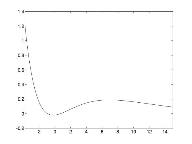
Figure 1: The potential, equation (58), is plotted against $\phi$ for $\xi=0.1$, $A=B=1$. When $x=e^{-\xi\phi}\approx x_{a}$ then the field is close to the local maximum of $V(\phi)$ and the scale factor, $a(t)$ will be growing exponentially. As the universe evolves, the field rolls away from the local maximum and the expansion makes a smooth transition to powerlaw growth.

Thus this solution exhibits the properties of the two major inflationary models at different stages in its evolution. If $\xi\lesssim 0.2$ and $x_{o}\approx x_{a}$ then a large amount of exponential expansion is possible, with the number of e-foldings depending critically on $\xi$ and the ratio $x_{o}/x_{a}$. In figures (1) and (2) $V(\phi)$ and $a(t)$ are plotted for a representative set of parameter values. Physically, since $x_{a}$ is a local maximum, the potential is approximately flat when $x\approx x_{a}$. Thus both $x$ and $V(x)$ are changing slowly, leading to an era of quasi-exponential expansion. As $x$ moves further away from $x_{a}$ the potential becomes steeper and the era of powerlaw expansion begins.

For most values of $\xi$, the coefficients of only two of the three coefficients in $V(x)$, equation (58) are independent. However, when $\xi=\sqrt{3/2}$, $\sqrt{3/4}$ or $\sqrt{3/8}$ one of the terms in $V(x)$ drops out, leaving only two nonzero terms which may be chosen arbitrarily. In particular, when $\xi=\sqrt{3/4}$, the potential is

$$V(\phi)=\frac{3}{2}A^{2}\exp{(-\sqrt{3}\phi)}-3B^{2}\exp{(-2\sqrt{3}\phi)}.$$ (64)

which is the first two terms in the superstring motivated perturbation expansion, equation (2), with $\gamma=\sqrt{3}$.

5.3 Modified Powerlaw Inflation

The next case we treat is superficially similar to the last, with

$$H(x)=Ax+Bx^{2},\quad B>0$$ (65)

but the evolution we derive is markedly different. The corresponding solution is

$$V(x) = A^{2}(3-2\xi^{2})x^{2}+2AB(3-4\xi^{2})x^{3}+B^{2}(3-8\xi^{2})x^{4}.$$ (66)

$$a(x) = a_{o}\left[\frac{x_{o}^{2}(A+2Bx)}{x^{2}(A+2Bx_{o})}\right]^{1/4\xi^{2}}$$ (67)

$$t(x) = \frac{1}{A\xi^{2}}\left[\frac{1}{2}\left(\frac{1}{x}-\frac{1}{x_{o}}\right)-\frac{B}{A}\log{\left(\frac{x_{o}(A+2Bx)}{x(A+2Bx_{o})}\right)}\right]$$ (68)

For this choice of $H(x)$, $V(x)\rightarrow\infty$ as $x\rightarrow\infty$ and $\xi\leq\sqrt{3/8}$. For other values of $\xi$, $V(x)$ is negative for large $x$. When $\sqrt{3/8}<\xi<\sqrt{3/2}$ the potential has a local maximum at

$$x_{a}=\frac{A}{B}\frac{2\xi^{2}-3}{3-8\xi^{2}}$$ (69)

but for $\xi\geq\sqrt{3/2}$, $V(x)<0$ for all allowable values of $x$. However, $a(t)$ is always increasing and there are no solutions for which the universe reaches a maximum size and then contracts back to a future singularity. This solution starts from a singularity though, since in the limit $x\rightarrow\infty$,

$$t=\frac{1}{A\xi^{2}}\left[\frac{B}{A}\log{\left(\frac{A+2Bx_{o}}{2Bx_{o}}\right)}-\frac{1}{2x_{o}}\right],\quad a=0.$$ (70)

In this instance, the logarithmic term in $a(x)$, never dominates and the expansion is always approximately powerlaw. Because this exact solution implicitly requires the value of $\dot{\phi}$ to be large when it is in the region containing the local maximum, the conditions that gave rise to a period of exponential expansion for the solution given by equations (59) and (60) are not be satisfied in this case. Of course the possibility of a period of exponential expansion in the general solution to the potential, equation (66), is not ruled out.

For this solution

$$\epsilon(x)=2\xi^{2}\left(\frac{A+2Bx}{A+Bx}\right)^{2}.$$ (71)

If $\xi>\sqrt{1/2}$, $\epsilon>1$ and there is no inflationary phase. Alternatively, if $\xi<\sqrt{1/8}$ the solution is inflationary at all times. For intermediate values of $\xi$, the inflationary era will be preceeded by a period of powerlaw expansion, $a\propto t^{p}$, but with $p<1$.

Again, there are three special cases for which one of the terms in $V(x)$ is zero, and a potential with two terms and independent coefficients results.

5.4 Exact solution for a superstring motivated potential

Starting from $H=Ax-Bx^{3}$, we find the potential,

$$V(x)=A^{2}(3-2\xi^{2})x^{2}+6AB(2\xi^{2}-1)x^{4}+3B^{2}(1-6\xi^{2})x^{6},$$ (72)

which has the form of the perturbation expansion suggested by superstring theory, equation (2), for all values of $\xi$.

$$a(x) = a_{o}\left[\frac{x_{o}^{3}(A-3Bx^{2})}{x^{3}(A-3Bx_{o}^{2})}\right]^{1/6\xi^{2}}$$ (73)

$$t(x) = \frac{1}{2A\xi^{2}}\left\{\frac{1}{x}-\frac{1}{x_{o}}+\frac{C}{2}\log{\left[\frac{(1-Cx)(1+Cx_{o})}{(1-Cx_{o})(1+Cx)}\right]}\right\}$$ (74)

where $C=\sqrt{3B/A}$.

For all $\xi$ there is a local maximum at $x=1/C$. For $x_{o}>1/C$, $x$ will increase as the universe evolves, and it will eventually reach a maximum size and collapse towards a singularity. For $x_{o}<1/C$, the expansion will continue indefinitely. If $x_{o}\approx 1/C$ then $a(t)$ will initially be approximately exponential, giving way to powerlaw behaviour at later times.

Again, there are three special values of $\xi$ for which one of the terms drops out of the potential. In particular, when $\xi=1/\sqrt{2}$, the potential is

$$V(\phi)=2A^{2}\exp{(-\sqrt{2}\phi)}-6B^{2}\exp{(-3\sqrt{2}\phi)}$$ (75)

and $\gamma=\sqrt{2}$, the value derived from superstring theory, although the term in $\exp{(-2\sqrt{2}\phi)}$ is missing.

Setting $H=Ax+Bx^{3}$ gives similar results to those found for $H=A+Bx^{2}$. The potential and the scale factor are found simply by changing the sign of $B$ in equations (72) and (73). The time, $t(x)$ is

$$t(x)=\frac{1}{2A\xi^{2}}\left[\frac{1}{x}-\frac{1}{x_{o}}+C\left(\tan^{-1}{(x)}-\tan^{-1}{(x_{o})}\right)\right]$$ (76)

This model with begins with a singularity, expands indefinitely and can have a mixture of non-inflationary and powerlaw expansion, depending on the value of $\xi$.

6 Discussion

We have found a number of new, exact scalar field cosmologies by deriving the potential that produces a specified form of the density, $\rho$, or the Hubble parameter, $H$. The technique used here typically does not produce a complete solution for a given potential. In particular, the solutions presented in this paper do not allow the initial value of $\dot{\phi}$ to be chosen arbitrarily. However, it is easy to apply and a large number of potentials can be examined and interesting examples isolated, which can then be studied with more complicated analytic or numerical methods.

In curved Robertson Walker spacetimes, we find a mixture of exact inflationary and non-inflationary models. We generalise solutions previously found by Özer and Taha [11] and develop analagous results for a universe with negative spatial curvature.

In flat spacetime we have presented exact solutions that have several distinct phases, distinguished by the properties of the scale factor, $a(t)$. As well as models with a smooth transition between inflationary and non-inflationary expansion, we have found instances where the inflationary growth is a combination of exponential and powerlaw expansion. We are not aware of any other exact scalar field cosmologies that are of a comparable complexity and diversity. If a realistic model possessed these properties, the resulting spectrum of primordial density perturbations would be comparatively complex, assuming that there is not so much powerlaw growth that the fluctuations produced during the era of exponential expansion are shifted beyond the present horizon.

We have concentrated on solutions with relatively simple potentials but the method used here can be used to generate an arbitrary number of exact solutions where the potential consists of exponential terms. While we can find only a handful of such solutions in curved spacetime, the simple relationship between $H$ and $V(x)$ when $k=0$, equation (48), means that large numbers of exact solutions can be obtained in flat spacetime and we have not exhausted their possibilities in this paper.

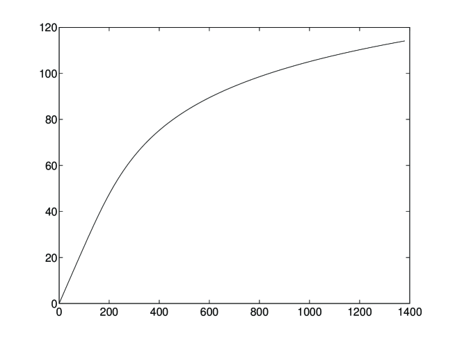
Figure 2: The scale factor, $\log{a(t)}$, is plotted against the time $t$ for a model where the potential has the specific form illustrated in Figure (1) and $x_{o}=0.98x_{a}$. When $t\lesssim 200$, $\log{a}$ is approximately proportional to the time, $t$ and the universe is growing exponentially with powerlaw inflation taking place at later times. At larger values of $\xi$ the amount of exponential expansion is reduced, but the transition to powerlaw growth is more abrupt.

References

- [1] Guth A H 1981 Phys. Rev. D 23 347–56
- [2] Albrecht A and Steinhardt P J 1982 Phys. Rev. Lett. 48 1220–3
- [3] Linde A D 1982 Phys. Lett. B 108 389–93
- [4] Salam A and Sezgin E 1984 Phys. Lett. B 147 47–51
- [5] Fradkin E S and Tseytlin A A 1985 Phys. Lett. B 158 316–22
- [6] Callan C G, Friedan D, Martinec E J and Perry M J 1985 Nuc. Phys. B 262 593–609
- [7] Callan C G, Klebanov I R and Perry M J 1986 Nuc. Phys. B 278 78–90
- [8] Gross D J and Sloan J H 1987 Nuc. Phys. B 291 41–89
- [9] Halliwell J J 1987 Nuc. Phys. B 286 729–50
- [10] Campbell B A, Linde A and Olive K A 1991 Nuc. Phys. B 355 146-61
- [11] Özer M and Taha M O 1992 Phys. Rev. D 45 997–9
- [12] Lucchin F and Matarrese S 1985 Phys. Rev. D 32 1316–22
- [13] Casas J A, García-Bellido J and Quirós M 1991 Nuc. Phys. B 361 713-28
- [14] García-Bellido J and Quirós M 1992 Nuc. Phys. B 368 463-78
- [15] Brustein R and Steinhardt P J 1993 Phys. Lett. B 302 196-201
- [16] Barrow J D, Burd A B and Lancaster D 1986 Class. Quantum Grav. 3 551–67
- [17] Barrow J 1987 Phys. Lett. B 187 12–6
- [18] Burd A B and Barrow J D 1988 Nuc. Phys. B 308 929–45
- [19] Yokoyama J and Maeda K 1988 Phys. Lett. B 207 31–5
- [20] Muslimov A G 1990 Class. Quantum Grav. 7 231–7
- [21] Liddle A 1989 Phys. Lett. B 220 502–8
- [22] Ratra B 1992 Phys. Rev. D 45 1913–52
- [23] Salopek D S and Bond J R 1990 Phys. Rev. D 42 3936–62
- [24] Lidsey J 1992 Class. Quantum Grav. 9 1239–53
- [25] de Ritis R, Marmo G, Platania G, Rubano C, Scudellaro P and Stornaiolo C 1990 Phys. Rev. D 42 1091–7
- [26] de Ritis R, Marmo G, Platania G, Rubano C, Scudellaro P and Stornaiolo C 1990 Phys. Lett. A 149 79–83
- [27] de Ritis R, Platania G, Rubano C and Sabatino R 1991 Phys. Lett. A 161 230–5
- [28] Abbott L F and Wise M B 1984 Nuc. Phys. B 244 541–8
- [29] Lucchin F and Matarrese S 1985 Phys.Lett. B 164 282–6
- [30] Barrow J D 1990 Phys. Lett. B 235 40–3
- [31] Barrow J D and Saich P 1990 Phys. Lett. B 249 406–9
- [32] Kolb E W and Turner M S 1990 The Early Universe vol. 69 of Frontiers in Physics (Addison Wesley, Redwood City, California)
- [33] Linde A D 1990 Particle Physics and Inflationary Cosmology vol. 5 of Contemporary Concepts in Physics (Harwood Academic Publishers, Chur, Switzerland)
- [34] Lidsey J 1991 Phys. Lett. B 273 42–6
- [35] Misner C W, Thorne K S and Wheeler J A 1973 Gravitation (W H Freeman, New York)
- [36] Ellis G F R and Madesn M S 1991 Class. Quantum Grav. 8 667–76
- [37] Ellis G F R, Lyth D H and Mijić M 1991 Phys. Lett. B 271 52–60
- [38] Halliwell J J 1987 Phys. Lett. B 185 341–4