From the Big Bang Theory to the Theory of a Stationary Universe

Abstract

We consider chaotic inflation in the theories with the effective potentials which at large $\phi$ behave either as $\phi^{n}$ or as $e^{\alpha\phi}$. In such theories inflationary domains containing sufficiently large and homogeneous scalar field $\phi$ permanently produce new inflationary domains of a similar type. This process may occur at densities considerably smaller than the Planck density. Self-reproduction of inflationary domains is responsible for the fundamental stationarity which is present in many inflationary models: properties of the parts of the Universe formed in the process of self-reproduction do not depend on the time when this process occurs. We call this property of the inflationary Universe local stationarity.

In addition to it, there may exist either a stationary distribution of probability $P_{c}$ to find a given field $\phi$ at a given time at a given point, or a stationary distribution of probability $P_{p}$ to find a given field $\phi$ at a given time in a given physical volume. If any of these distributions is stationary, we will be speaking of a global stationarity of the inflationary Universe.

In all realistic inflationary models which are known to us the probability distribution $P_{c}$ is not stationary. On the other hand, investigation of the probability distribution $P_{p}$ describing a self-reproducing inflationary Universe shows that the center of this distribution moves towards greater and greater $\phi$ with increasing time. It is argued, however, that the probability of inflation (and of the self-reproduction of inflationary domains) becomes strongly suppressed when the energy density of the scalar field approaches the Planck density. As a result, the probability distribution $P_{p}$ rapidly approaches a stationary regime, which we have found explicitly for the theories ${\lambda\over 4}\phi^{4}$ and $e^{\alpha\phi}$. In this regime the relative fraction of the physical volume of the Universe in a state with given properties (with given values of fields, with a given density of matter, etc.) does not depend on time, both at the stage of inflation and after it.

Each of the two types of stationarity mentioned above constitutes a significant deviation of inflationary cosmology from the standard Big Bang paradigm. We compare our approach with other approaches to quantum cosmology, and illustrate some of the general conclusions mentioned above with the results of a computer simulation of stochastic processes in the inflationary Universe.

I Introduction

The standard Big Bang theory asserts that the Universe was born at some moment $t=0$ about 15 billion years ago, in a state of infinitely large density and temperature. With the rapid expansion of the Universe the average energy of particles, given by the temperature, decreased rapidly, and the Universe became cold. This theory became especially popular after the discovery of the microwave background radiation. However, by the end of the 70’s it was understood that this theory is hardly compatible with the present theory of elementary particles (primordial monopole problem, Polonyi fields problem, gravitino problem, domain wall problem) and it has many internal difficulties (flatness problem, horizon problem, homogeneity and isotropy problems, etc.).

Fortunately, all these problems can be solved simultaneously in the context of a relatively simple scenario of the Universe evolution — the inflationary Universe scenario b13 –b90 , MyBook . The main idea of this scenario is that the Universe at the very early stages of its evolution expanded quasi-exponentially (the stage of inflation) in a state with energy density dominated by the potential energy density $V(\phi)$ of some scalar field $\phi$. This rapid expansion made the Universe flat, homogeneous and isotropic and decreased exponentially the density of monopoles, gravitinos and domain walls. Later, the potential energy density of the scalar field transformed into thermal energy, and still later, the Universe was correctly described by the standard hot Universe theory predicting the existence of the microwave background radiation.

The first models of inflation were formulated in the context of the Big Bang theory. Their success in solving internal problems of this theory apparently removed the last doubts concerning the Big Bang cosmology. It remained almost unnoticed that during the last ten years inflationary theory changed considerably. It has broken an umbilical cord connecting it with the old Big Bang theory, and acquired an independent life of its own. For the practical purposes of describing the observable part of our Universe one may still speak about the Big Bang, just as one can still use Newtonian gravity theory to describe the Solar system with very high precision. However, if one tries to understand the beginning of the Universe, or its end, or its global structure, then some of the notions of the Big Bang theory become inadequate. For example, one of the main principles of the Big Bang theory is the homogeneity of the Universe. The assertion of homogeneity seemed to be so important that it was called “the cosmological principle” Peebles . Indeed, without using this principle one could not prove that the whole Universe appeared at a single moment of time, which was associated with the Big Bang. So far, inflation remains the only theory which explains why the observable part of the Universe is almost homogeneous. However, almost all versions of inflationary cosmology predict that on a much larger scale the Universe should be extremely inhomogeneous, with energy density varying from the Planck density to almost zero. Instead of one single Big Bang producing a single-bubble Universe, we are speaking now about inflationary bubbles producing new bubbles, producing new bubbles, ad infinitum b19 ; b20 . Thus, recent development of inflationary theory considerably modified our cosmological paradigm MyBook . In order to understand better this modification, we should remember the main turning points in the evolution of the inflationary theory.

The first semi-realistic version of inflationary cosmology was suggested by Starobinsky b14 . However, originally it was not quite clear what should be the initial state of the Universe in this scenario. Inflation in this model could not occur if the Universe was hot from the very beginning. To solve this problem, Zeldovich in 1981 suggested that the inflationary Starobinsky Universe was created “from nothing” Zeld . This idea, which is very popular now NothVil –b59 , at that time seemed too extravagant, and most cosmologists preferred to study inflation in more traditional context of the hot Universe theory.

One of the most important stages of the development of the inflationary cosmology was related to the old inflationary Universe scenario by Guth b15 . This scenario was based on three fundamental propositions:

1. The Universe initially expands in a state with a very high temperature, which leads to the symmetry restoration in the early Universe, $\phi(T)=0$, where $\phi$ is some scalar field driving inflation (the inflaton field).

2. The effective potential $V(\phi,T)$ of the scalar field $\phi$ has a deep local minimum at $\phi=0$ even at a very low temperature T. As a result, the Universe remains in a supercooled vacuum state $\phi=0$ (false vacuum) for a long time. The energy-momentum tensor of such a state rapidly becomes equal to $T_{\mu\nu}=g_{\mu\nu}V(0)$, and the Universe expands exponentially (inflates) until the false vacuum decays.

3. The decay of the false vacuum proceeds by forming bubbles containing the field $\phi_{0}$ corresponding to the minimum of the effective potential $V(\phi)$. Reheating of the Universe occurs due to the bubble-wall collisions.

The main idea of the old inflationary Universe scenario was very simple and attractive, and the role of the old inflationary scenario in the development of modern cosmology was extremely important. Unfortunately, as it was pointed out by Guth in b15 , this scenario had a major problem. If the rate of the bubble formation is bigger than the speed of the Universe expansion, then the phase transition occurs very rapidly and inflation does not take place. On the other hand, if the vacuum decay rate is small, then the Universe after the phase transition becomes unacceptably inhomogeneous.

All attempts to suggest a successful inflationary Universe scenario failed until cosmologists managed to surmount a certain psychological barrier and renounce the aforementioned assumptions, while retaining the main idea of ref. b15 that the Universe has undergone inflation during the early stages of its evolution. The invention of the new inflationary Universe scenario b16 marked the departure from the assumptions (2), (3). Later it was shown that the assumption (1) also does not hold in all realistic models known so far, for two main reasons. First of all, the time which is necessary for the field $\phi$ to roll down to the minimum of $V(\phi,T)$ is typically too large, so that either inflation occurs before the field rolls to the minimum of $V(\phi,T)$, or it does not occur at all. On the other hand, even if the field $\phi$ occasionally was near the minimum of $V(\phi,T)$ from the very beginning, inflation typically starts very late, when thermal energy drops from $M^{4}_{p}$ down to $V(0,T)$. In all realistic models of inflation $V(0,T)<10^{-10}M^{4}_{p}$, hence inflation may start in a state with $\phi=0$ not earlier than at $t\sim 10^{4}M^{-1}_{p}$. During such a time a typical closed Universe would collapse before the conditions necessary for inflation could be realized MyBook .

The assumption (1) was finally given up with the invention of the chaotic inflation scenario b17 . The main idea of this scenario was to abandon the assumption that the Universe from the very beginning was hot, and that the initial state of the scalar field should correspond to a minimum of its effective potential. Instead of that, one should study various initial distributions of the scalar field $\phi$, including those which describe the scalar field outside of its equilibrium state, and investigate in which case the inflationary regime may occur.

In other words, the main idea of chaotic inflation was to remove all unnecessary restrictions on inflationary models inherited from the old theory of the hot Big Bang. In fact, the first step towards this liberation was already made when it was suggested to consider quantum creation of inflationary Universe from nothing Zeld –b59 . Chaotic inflation naturally incorporates this idea b56 , but it is more general: inflation in this scenario can also appear under a more traditional assumption of initial cosmological singularity.

Thus, the main idea of chaotic inflation is very simple and general. One should study all possible initial conditions without insisting that the Universe was in a state of thermal equilibrium, and that the field $\phi$ was in the minimum of its effective potential from the very beginning. However, this idea strongly deviated from the standard lore and was psychologically difficult to accept. Therefore, for many years almost all inflationary model builders continued the investigation of the new inflationary scenario and calculated high-temperature effective potentials in all theories available. It was argued that every inflationary model should satisfy the so-called ‘thermal constraints’ TurStein , that chaotic inflation requires unnatural initial conditions, etc.

At present the situation is quite opposite. If anybody ever discusses the possibility that inflation is initiated by high-temperature effects, then typically the purpose of such a discussion is to show over and over again that this idea does not work (see e.g. Thermal ), even though some exceptions from this rule might still be possible. On the other hand, there are many theories where one can have chaotic inflation (for a review see MyBook ).

A particularly simple realization of this scenario can be achieved in the theory of a massive scalar field with the effective potential ${m^{2}\over 2}\phi^{2}$, or in the theory ${\lambda\over 4}\phi^{4}$, or in any other theory with an effective potential which grows as $\phi^{n}$ at large $\phi$ (whether or not there is a spontaneous symmetry breaking at small $\phi$). Therefore a lot of work illustrating the basic principles of chaotic inflation was carried out in the context of these simple models. However, it would be absolutely incorrect to identify the chaotic inflation scenario with these models, just as it would be incorrect to identify new inflation with the Coleman-Weinberg theory. The dividing line between the new inflation and the chaotic inflation was not in the choice of a specific class of potentials, but in the abandoning of the idea that the high-temperature phase transitions should be a necessary pre-requisite of inflation.

Indeed, already in the first paper where the chaotic inflation was proposed b17 , it was emphasized that this scenario can be implemented not only in the theories $\sim\phi^{n}$, but in any model where the effective potential is sufficiently flat at some $\phi$. In the second paper on chaotic inflation Chaot2 this scenario was implemented in a model with an effective potential of the same type as those used in the new inflationary scenario. It was explained that the standard scenario based on high-temperature phase transitions cannot be realized in this theory, whereas the chaotic inflation can occur there, either due to the rolling of the field $\phi$ from $\phi>1$, or due to the rolling down from the local maximum of the effective potential at $\phi=0$. In ExpChaot it was pointed out that chaotic inflation can be implemented in many theories including the theories with exponential potentials $\sim e^{\alpha\phi}$ with $\alpha<\sqrt{16\pi}$. This is precisely the same class of theories which two years later was used in Exp to obtain the power law inflation Power . The class of models where chaotic inflation can be realized includes also the models based on the $SU(5)$ grand unified theory MyBook , the $R^{2}$ inflation (modified Starobinsky model) StChaot , supergravity-inspired models with polynomial and non-polynomial potentials Supergr , ‘natural inflation’ Natural , ‘extended inflation’ b90 , EtExInf , ‘hybrid inflation’ Axions , etc.

Several years ago it was discovered that chaotic inflation in many models including the theories $\phi^{n}$ has a very interesting property, which will be discussed in the present paper b19 ; b20 . If the Universe contains at least one inflationary domain of a size of horizon ($h$-region) with a sufficiently large and homogeneous scalar field $\phi$, then this domain will permanently produce new $h$-regions of a similar type. During this process the total physical volume of the inflationary Universe (which is proportional to the total number of $h$-regions) will grow indefinitely. The process of self-reproduction of inflationary domains occurs not only in the theories with the effective potentials growing at large $\phi$ b19 ; b20 , but in some theories with the effective potentials used in old, new and extended inflation scenarios as well b51 ; b52 ; b62 ; EtExInf . However, in the models with the potentials growing at large $\phi$ the existence of this effect was most unexpected, and it leads to especially interesting cosmological consequences MyBook .

The process of the self-reproduction of inflationary Universe represents a major deviation of inflationary cosmology from the standard Big Bang theory. In this paper we will make an attempt to relate the existence of this process to the long-standing problem of finding a true gravitational vacuum, some kind of a stationary ground state of a system, similar to the vacuum state in Minkowski space or to the ground state in quantum statistics.

A priori it is not quite clear that a stationary ground state in quantum gravity may exist at all. This question becomes especially pronounced being applied to quantum cosmology. Indeed, how can one expect that at the quantum level there exists any kind of stationary state if all nontrivial classical cosmological solutions are non-stationary?

A possible (and rather paradoxical) answer to this question is suggested by the observation made in DeWitt that the wave function of the whole Universe does not depend on time, since the total Hamiltonian, including the contribution from gravitational interactions, identically vanishes. This observation has led several authors to the idea of using scale factor of the Universe instead of time, which implied existence of many strange phenomena like time reversal and resurrection of the dead at the moment of maximal expansion of a closed Universe. The resolution of the paradox was suggested by DeWitt in DeWitt (see also discussion of this question in Page , MyBook ). We do not ask why the Universe evolves in time measured by some nonexistent observer outside our Universe; we just ask why we see it evolving in time. At the moment when we make our observations, the Universe is divided into two pieces: an observer with its measuring devices and the rest of the Universe. The wave function of the rest of the Universe does depend on the time shown by the clock of the observer. Thus, at the moment we start observing the Universe it ceases being static and appears to us time-dependent.

From this discussion it follows that the condition of time-independence is not strong enough to pick up a unique wave function of the Universe corresponding to its ground state: each wave function satisfying the Wheeler-DeWitt equation (being interpreted as a Schrödinger equation for the wave function of the Universe) is time-independent. One way to deal with this problem is to assume that the standard Euclidean methods, which help to find the wave function of the vacuum state in ordinary quantum theory of matter fields, will work for the wave function of the Universe as well. This assumption was made by Hartle and Hawking HH . Another way is to look for a possibility that with an account taken of quantum effects our Universe in some cases may approach a stationary state, which could be called the ground state.

In some cases these two approaches lead to the same results. For example, the square of the Hartle-Hawking wave function correctly describes $P_{c}(\phi,t)$, the stationary probability distribution for finding the scalar field $\phi$ at a given time in a given point of de Sitter space with the Hubble constant $H\gg m$, where $m$ is the mass of the scalar field b60 –Star . Here the subscript $c$ in $P_{c}(\phi,t)$ means that the distribution is considered in comoving coordinates, which do not take into account the exponential growth of physical volume of the Universe. However, later it was realized that no stationary solutions for $P_{c}(\phi,t)$ can exist in realistic versions of inflationary cosmology b19 ; b20 . The reason is that the condition $H\gg m$ is strongly violated near the minimum of the effective potential $V(\phi)$ corresponding to the present state of the Universe. Indeed, this condition could be satisfied at present only if the Compton wavelength of the inflaton field were larger than the size of the observable part of the Universe $\sim H^{-1}$ and its mass were smaller than $10^{-22}$ eV. In all realistic models of inflation this condition is violated by more than thirty orders of magnitude.

Fortunately, another kind of stationarity may exist in many models of the inflationary Universe due to the process of self-reproduction of the Universe MyBook ; b19 ; b20 . The properties of inflationary domains formed during the self-reproduction of the Universe do not depend on the moment of time at which each such domain is formed; they depend only on the value of the scalar fields inside each domain, on the average density of matter in this domain and on the physical length scale. For example, all domains of our Universe with energy density $\rho_{0}\sim 10^{-29}g\cdot cm^{-3}$ filled with the same scalar fields look alike on the same length scale, independently of the time when they were formed. This kind of stationarity, as opposed to the stationarity of the distribution $P_{c}(\phi,t)$ corresponding to the Hartle-Hawking wave function, cannot be described in the minisuperspace approach. Hopefully, the existence of this stationarity (which implies that our Universe has a fractal structure) will eventually help us to find the most adequate wave function describing the self-reproducing inflationary Universe.

One way to describe this kind of stationarity is to use the methods developed in the theory of fractals. This question was studied in ArVil in application to the theories where inflation occurs near a local maximum of the effective potential $V(\phi)$. In this case the expansion of the whole Universe, though eternal, is almost uniform — the scale factor of the Universe $a(t)$ grows as $e^{Ht}$, where $H$ almost does not depend on the value of the inflaton field $\phi$. This makes it possible to factor out the trivial overall expansion factor, and come to a time-independent fractal structure without taking into account the difference between $P_{c}(\phi,t)$ and $P_{p}(\phi,t)$. Unfortunately, it is rather difficult to apply these methods to the most interesting and general case where the effective potential $V(\phi)$ considerably changes during inflation. This is the case, for example, in the theories with potentials $\phi^{n}$ and $e^{\alpha\phi}$ b17 . In such theories one has to treat the boundary conditions much more carefully in order to find the correct rate of the volume growth.

Another approach is to investigate the probability distribution $P_{p}(\phi,t)$, which takes into account the exponential growth of the volume of domains filled by the inflaton field $\phi$ b19 . Solutions for this probability distribution were first examined in b19 ; b20 for the case of chaotic inflation in the theories with potentials $\phi^{n}$. It was shown that if the initial value of the scalar field $\phi$ is greater than some critical value $\phi^{*}$, then the probability distribution $P_{p}(\phi,t)$ permanently moves to greater and greater fields $\phi$. This process continues until the maximum of the distribution $P_{p}(\phi,t)$ approaches the field $\phi_{p}$, at which the effective potential of the field becomes of the order of Planck density $M_{p}^{4}$, where the standard methods of quantum field theory in a curved classical space are no longer valid. By the methods used in b19 ; b20 it was impossible to check whether $P_{p}(\phi,t)$ asymptotically approaches any stationary regime in the classical domain $\phi<\phi_{p}$.

More generally, one may consider the probability distribution $P_{p}(\phi,t|\chi)$, which shows the fraction of volume of the Universe filled by the field $\phi$ at the time $t$, if originally, at the time $t=0$, the part of the Universe which we study was filled by the field $\phi_{0}=\chi$. Several important steps towards the investigation of this probability distribution in the theories $\phi^{n}$ were made by Nambu and Sasaki Nambu (see also SNN ; NewStationary ) and by Mijić Mijic . Their papers contain many beautiful insights, and we will use many results obtained by these authors. However, Mijić Mijic did not have a purpose in obtaining a complete expression for the stationary distribution $P_{p}(\phi,t)$. The corresponding expressions were obtained for various potentials $V(\phi)$ in Nambu . Unfortunately, the stationary distribution $P_{p}(\phi,t)$ obtained in Nambu was almost entirely concentrated at $\phi\gg\phi_{p}$, i.e. at $V(\phi)\gg M_{p}^{4}$, where the methods used in Nambu were inapplicable.

In the present paper we will argue that the self-reproduction of the inflationary Universe effectively kills itself at densities approaching the Planck density. This leads to the existence of a stationary probability distribution $P_{p}(\phi,t)$ concentrated entirely at sub-Planckian densities $V(\phi)<M_{p}^{4}$ in a wide class of theories leading to chaotic inflation MezhLinSmall ; MezhLin .

The new cosmological paradigm based on inflationary cosmology is very unusual. Instead of the Universe looking like an expanding ball of fire, we are considering now a huge fractal consisting of many inflating balls producing new balls, producing new balls, etc. In order to make the new cosmological concepts more visually clear, we include in this paper a series of figures which show the results of computer simulations of stochastic processes in the inflationary Universe LinLin .

The plan of the paper is the following. In Section II we give a short review of chaotic inflation. We discuss the generation of density perturbations and explain how they lead to the process of self-reproduction of the Universe. In Section III we discuss the interrelations between stochastic and Euclidean approaches to quantum cosmology and explain the main advantages of the probability distribution $P_{p}(\phi,t)$ for the description of the global structure of inflationary Universe. Section IV briefly describes the results of the computer simulation of stochastic processes in inflationary Universe. Section V contains the basics of our approach to finding a stationary probability distribution $P_{p}(\phi,t|\chi)$. In Section VI we describe the analogous investigation for a different parametrization of time. Section VII contains a general discussion of the consequences of our results, which are summarized in a short concluding Section VIII.

To simplify our notation, throughout this paper we will use the system of units where $M_{p}=1$.

II Self-Reproducing Chaotic Inflationary Universe

II.1 Chaotic Inflation

We will begin our discussion of chaotic inflation with the simplest model based on the theory of a scalar field $\phi$ minimally coupled to gravity, with the Lagrangian

$$L=\frac{1}{16\pi}R+\frac{1}{2}\partial_{\mu}\phi\partial^{\mu}\phi-V(\phi)\ .$$ (1)

Here $G=M^{-2}_{p}=1$ is the gravitational constant, $R$ is the curvature scalar, and $V(\phi)$ is the effective potential of the scalar field. If the classical field $\phi$ is sufficiently homogeneous in some domain of the Universe (see below), then its behavior inside this domain is governed by the equations

$$\ddot{\phi}+3H\dot{\phi}=-dV/d\phi\ ,$$ (2)

$$H^{2}+\frac{k}{a^{2}}=\frac{8\pi}{3}\,\left(\frac{1}{2}\dot{\phi}^{2}+V(\phi)\right)\ .$$ (3)

Here $H={\dot{a}}/a,a(t)$ is the scale factor of the Universe, $k=+1,-1,$ or $0$ for a closed, open or flat Universe, respectively.

The simplest version of the theory (1) is the theory of a massive noninteracting scalar field with the effective potential $V(\phi)=\frac{1}{2}m^{2}\phi^{2}$, where $m$ is the mass of the scalar field $\phi$, $m\ll 1$. If the field $\phi$ initially is sufficiently large, $\phi\gg 1$, then one can show that the functions $\phi(t)$ and $a(t)$ rapidly approach the asymptotic regime

$$\phi(t)=\phi_{0}-\frac{m}{2(3\pi)^{1/2}}t\ ,$$ (4)

$$a(t)=a_{0}\exp\left(2\pi\left(\phi^{2}_{0}-\phi^{2}(t)\right)\right)\ .$$ (5)

Note that in this regime the second derivative of the scalar field in eq. (2) and the term $k/a^{2}$ in (3) can be neglected. The last statement means that the Universe becomes locally flat.

According to (4) and (5), during the time $\tau\sim\phi/m$ the relative change of the field $\phi$ remains small, the effective potential $V(\phi)$ changes very slowly and the Universe expands quasi-exponentially:

$$a(t+\Delta t)\sim a(t)\exp(H\Delta t)$$ (6)

for $\Delta t\leq\tau=\phi/m$. Here

$$H=2\sqrt{\frac{\pi}{3}}\,m\phi\ .$$ (7)

Note that $\tau\gg H^{-1}$ for $\phi\gg 1$.

The regime of the slow rolling of the field $\phi$ and the quasi-exponential expansion (inflation) of the Universe ends at $\phi\mathrel{\hbox{\hbox to0.0pt{\hbox{\lower 4.0pt\hbox{$\sim$}}\hss}\hbox{$<$}}}\phi_{e}$. In the theory under consideration, $\phi_{e}\sim 0.2$. At $\phi\leq\phi_{e}$ the field $\phi$ oscillates rapidly, and if this field interacts with other matter fields (which are not written explicitly in eq. (1)), its potential energy $V(\phi)\sim\frac{m^{2}\phi_{e}^{2}}{2}\sim{m^{2}\over 50}$ is transformed into heat. The reheating temperature $T_{R}$ may be of the order $m^{1/2}$ or somewhat smaller, depending on the strength of the interaction of the field $\phi$ with other fields. It is important that $T_{R}$ does not depend on the initial value $\phi_{0}$ of the field $\phi$. The only parameter which depends on $\phi_{0}$ is the scale factor $a(t)$, which grows $e^{2\pi\phi^{2}_{0}}$ times during inflation.

All results obtained above can be easily generalized for the theories with more complicated effective potentials. For example, during inflation in the theories with $V(\phi)=\frac{\lambda}{n}\,\phi^{n}$ one has

$$\phi^{4-n\over 2}(t)=\phi^{4-n\over 2}_{0}-\frac{4-n}{2}\,\sqrt{\frac{n\lambda}{24\pi}}\ t\ \ \ \ \mbox{for}\ n\not=4\ ,$$ (8)

$$\phi(t)=\phi_{0}\ \exp\left(-\sqrt{\lambda\over 6\pi}\,t\right)\ \ \ \ \ \mbox{for}\ n=4\ .$$ (9)

For all $n$,

$$a(t)=a_{0}\exp\left({4\pi\over n}(\phi^{2}_{0}-\phi^{2}(t))\right)\ .$$ (10)

Inflation ends at

$$\phi_{e}\sim{n\over 4\sqrt{3\pi}}\ .$$ (11)

Note, that in all realistic models of elementary particles spontaneous symmetry breaking occurs on a scale which is many orders of magnitude smaller than 1 (i.e. smaller than $M_{p}$). Therefore all results which we obtained remain valid in all theories which have potentials $V(\phi)\sim\frac{\lambda}{n}\,\phi^{n}$ at $\phi\mathrel{\hbox{\hbox to0.0pt{\hbox{\lower 4.0pt\hbox{$\sim$}}\hss}\hbox{$>$}}}1$, independently of the issue of spontaneous symmetry breaking which may occur in such theories at small $\phi$.

As was first pointed out in ExpChaot , chaotic inflation occurs as well in the theories with exponential effective potentials $V(\phi)={V_{0}}\ {e^{\alpha\phi}}$ for sufficiently small $\alpha$. It was shown later Exp that in the theories with

$$V(\phi)={V_{0}}\ {e^{\alpha\phi}}$$ (12)

the Einstein equations and equations for the scalar field have an exact solution:

$$\phi(t)=\phi_{0}-{2\over\alpha}\ \ln{t\over t_{0}}\ ,$$ (13)

$$a(t)=a_{0}\,t^{p},\ \ p=\frac{16\,\pi}{\alpha^{2}}\ .$$ (14)

Note that here we are dealing with the power law expansion of the Universe. It can be called inflation if $p\gg 1$, which implies that $\alpha\ll\sqrt{16\pi}\sim 7$ ExpChaot . In this case the Hubble constant $H$ almost does not change within the Hubble time $\sim H^{-1}$, and expansion looks quasiexponential, like in eq. (6). Inflation in the theory with the exponential potential never ends; it occurs at all $\phi$. In order to make this theory realistic, one should assume that at small $\phi$ the effective potential becomes steep and inflation ends at $\phi<\phi_{e}$. Without any loss of generality one can assume that $\phi_{e}=0$. In this case the parameter $V_{0}$ gives the value of the effective potential at the end of inflation.

II.2 Initial conditions for inflation

Let us consider first a closed Universe of initial size $\l\sim 1$ (in Planck units), which emerges from the space-time foam, or from singularity, or from ‘nothing’ in a state with the Planck density $\rho\sim 1$. Only starting from this moment, i.e. at $\rho\mathrel{\hbox{\hbox to0.0pt{\hbox{\lower 4.0pt\hbox{$\sim$}}\hss}\hbox{$<$}}}1$, can we describe this domain as a classical Universe. Thus, at this initial moment the sum of the kinetic energy density, gradient energy density, and the potential energy density is of the order unity:  ${1\over 2}\dot{\phi}^{2}+{1\over 2}(\partial_{i}\phi)^{2}+V(\phi)\sim 1$.

We wish to emphasize, that there are no a priori constraints on the initial value of the scalar field in this domain, except for the constraint ${1\over 2}\dot{\phi}^{2}+{1\over 2}(\partial_{i}\phi)^{2}+V(\phi)\sim 1$. Let us consider for a moment a theory with $V(\phi)=const$. This theory is invariant under the shift $\phi\to\phi+a$. Therefore, in such a theory all initial values of the homogeneous component of the scalar field $\phi$ are equally probable. Note, that this expectation would be incorrect if the scalar field should vanish at the boundaries of the original domain. Then the constraint ${1\over 2}(\partial_{i}\phi)^{2}\mathrel{\hbox{\hbox to0.0pt{\hbox{\lower 4.0pt\hbox{$\sim$}}\hss}\hbox{$<$}}}1$ would tell us that the scalar field cannot be greater than $1$ inside a domain of initial size $1$. However, if the original domain is a closed Universe, then it has no boundaries. (We will discuss a more general case shortly.)

The only constraint on the average amplitude of the field appears if the effective potential is not constant, but grows and becomes greater than the Planck density at $\phi>\phi_{p}$, where $V(\phi_{p})=1$. This constraint implies that $\phi\mathrel{\hbox{\hbox to0.0pt{\hbox{\lower 4.0pt\hbox{$\sim$}}\hss}\hbox{$<$}}}\phi_{p}$, but it does not give any reason to expect that $\phi\ll\phi_{p}$. This suggests that the typical initial value $\phi_{0}$ of the field $\phi$ in such a theory is

$$\phi_{0}\sim\phi_{p}\ .$$ (15)

Thus, we expect that typical initial conditions correspond to ${1\over 2}\dot{\phi}^{2}\sim{1\over 2}(\partial_{i}\phi)^{2}\sim V(\phi)=O(1)$. Note that if by any chance ${1\over 2}\dot{\phi}^{2}+{1\over 2}(\partial_{i}\phi)^{2}\mathrel{\hbox{\hbox to0.0pt{\hbox{\lower 4.0pt\hbox{$\sim$}}\hss}\hbox{$<$}}}V(\phi)$ in the domain under consideration, then inflation begins, and within the Planck time the terms ${1\over 2}\dot{\phi}^{2}$ and ${1\over 2}(\partial_{i}\phi)^{2}$ become much smaller than $V(\phi)$, which ensures continuation of inflation. It seems therefore that chaotic inflation occurs under rather natural initial conditions, if it can begin at $V(\phi)\sim 1$ MyBook ; b17 ; ExpChaot .

The assumption that inflation may begin at a very large $\phi$ has important implications. For example, in the theory (1) one has

$$\phi_{0}\sim\phi_{p}\sim m^{-1/2}\ .$$ (16)

Let us consider for definiteness a closed Universe of a typical initial size $O(1)$. Then, according to (5), the total size of the Universe after inflation becomes equal to

$$l\sim\exp\left(2\pi\phi^{2}_{0}\right)\sim\exp\left(\frac{2\pi}{m^{2}}\right)\ .$$ (17)

For $m\sim 10^{-6}$ (which is necessary to produce density perturbations $\frac{\delta{\rho}}{\rho}\sim 10^{-5}$, see below)

$$l\sim\exp\left(2\pi 10^{12}\right)>10^{10^{12}}cm\ .$$ (18)

Thus, according to this estimate, the smallest possible domain of the Universe of initial size $O(M_{p}^{-1})\sim 10^{-33}cm$ after inflation becomes much larger than the size of the observable part of the Universe $\sim 10^{28}cm$. This is the reason why our part of the Universe looks flat, homogeneous and isotropic. The same mechanism solves also the horizon problem. Indeed, any domain of the Planck size, which becomes causally connected within the Planck time, gives rise to the part of the Universe which is much larger than the part which we can see now.

In what follows we will return many times to our conclusion that the most probable initial value of the scalar field corresponds to $\phi\sim\phi_{p}$. There were many objections to it. Even though all these objections were answered many years ago MyBook ; ExpChaot , we need to discuss here one of these objections again. This is important for a proper understanding of the new picture of the evolution of the Universe in inflationary cosmology.

Assume that the Universe is not closed but infinite, or at least extremely large from the very beginning. (This objection does not apply to the closed Universe scenario discussed above.) In this case one could argue that our expectation that $\phi_{0}\sim\phi_{p}\gg 1$ is not very natural KolbTurn . Indeed, the conditions $(\partial_{i}\phi)^{2}\mathrel{\hbox{\hbox to0.0pt{\hbox{\lower 4.0pt\hbox{$\sim$}}\hss}\hbox{$<$}}}1$ and $\phi_{0}\sim\phi_{p}\gg 1$ imply that the field $\phi$ should be of the same order of magnitude $\phi\sim\phi_{p}\gg 1$ on a length scale at least as large as $\phi_{p}$, which is much larger than the scale of horizon $l\sim 1$ at the Planck time. But this is highly improbable, since initially (i.e., at the Planck time ) there should be no correlation between values of the field $\phi$ in different regions of the Universe separated from one another by distances greater than $1$. The existence of such correlation would violate causality. As it is written in KolbTurn , the scalar field $\phi$ must be smooth on a scale much greater than the scale of the horizon, which does not sound very chaotic.

The answer to this objection is very simple MyBook ; ExpChaot . We have absolutely no reason to expect that the overall energy density $\rho$ simultaneously becomes smaller than the Planck energy density in all causally disconnected regions of an infinite Universe, since that would imply the existence of an acausal correlation between values of $\rho$ in different domains of Planckian size $l_{p}\sim 1$. Thus, each such domain at the Planck time after its creation looks like an isolated island of classical space-time, which emerges from the space-time foam independently of other such islands. During inflation, each of these islands independently acquires a size many orders of magnitude larger than the size of the observable part of the Universe. A typical initial size of a domain of classical space-time with $\rho\mathrel{\hbox{\hbox to0.0pt{\hbox{\lower 4.0pt\hbox{$\sim$}}\hss}\hbox{$<$}}}1$ is of the order of the Planck length. Outside each of these domains the condition $\rho\mathrel{\hbox{\hbox to0.0pt{\hbox{\lower 4.0pt\hbox{$\sim$}}\hss}\hbox{$<$}}}1$ no longer holds, and there is no correlation between values of the field $\phi$ in different disconnected regions of classical space-time of size $1$. But such correlation is not necessary at all for the realization of the inflationary Universe scenario: according to the ‘no hair’ theorem for de Sitter space, a sufficient condition for the existence of an inflationary region of the Universe is that inflation takes place inside a region whose size is of order $H^{-1}$. In our case this condition is satisfied.

We wish to emphasize once again that the confusion discussed above, involving the correlation between values of the field $\phi$ in different causally disconnected regions of the Universe, is rooted in the familiar notion of a very large Universe that is instantaneously created from a singular state with $\rho=\infty$, and instantaneously passes through a state with the Planck density $\rho=1$. The lack of justification for such a notion is the very essence of the horizon problem. Now, having disposed of the horizon problem with the aid of the inflationary Universe scenario, we can possibly manage to familiarize ourselves with a different picture of the Universe. In this picture the simultaneous creation of the whole Universe is possible only if its initial size is of the order $1$, in which case no long-range correlations appear. Initial conditions should be formulated at the Planck time and on the Planck scale. Within each Planck-size island of the classical space-time, the initial spatial distribution of the scalar field cannot be very irregular due to the constraint $(\partial_{i}\phi)^{2}\mathrel{\hbox{\hbox to0.0pt{\hbox{\lower 4.0pt\hbox{$\sim$}}\hss}\hbox{$<$}}}1$. But this does not impose any constraints on the average values of the scalar field $\phi$ in each of such domains. One should examine all possible values of the field $\phi$ and check whether they could lead to inflation.

Note, that the arguments given above b17 ; ExpChaot suggest that initial conditions for inflation are quite natural only if inflation begins as close as possible to the Planck density. These arguments do not give any support to the models where inflation is possible only at densities much smaller than $1$. And indeed, an investigation of this question shows, for example, that a typical closed Universe where inflation is possible only at $V(\phi)\ll 1$ collapses before inflation begins. Thus, inflationary models of that type require fine-tuned initial conditions Piran , and apparently cannot solve the flatness problem.

Does this mean that we should forget all models where inflation may occur only at $V(\phi)\ll 1$? Does this mean, in particular, that the ‘natural inflation’ model is, in fact, absolutely unnatural?

As we will argue in the last section of this paper, it may be possible to rescue such models either by including them into a more general cosmological scenario (‘hybrid inflation’ Axions ), or by using some ideas of quantum cosmology, which we are going to elaborate.

II.3 Quantum Fluctuations and Density Perturbations

According to quantum field theory, empty space is not entirely empty. It is filled with quantum fluctuations of all types of physical fields. These fluctuations can be considered as waves of physical fields with all possible wavelengths, moving in all possible directions. If the values of these fields, averaged over some macroscopically large time, vanish, then the space filled with these fields seems to us empty and can be called the vacuum.

In the exponentially expanding Universe the vacuum structure is much more complicated. The wavelengths of all vacuum fluctuations of the scalar field $\phi$ grow exponentially in the expanding Universe. When the wavelength of any particular fluctuation becomes greater than $H^{-1}$, this fluctuation stops oscillating, and its amplitude freezes at some nonzero value $\delta\phi(x)$ because of the large friction term $3H\dot{\phi}$ in the equation of motion of the field $\phi$. The amplitude of this fluctuation then remains almost unchanged for a very long time, whereas its wavelength grows exponentially. Therefore, the appearance of such a frozen fluctuation is equivalent to the appearance of a classical field $\delta\phi(x)$ that does not vanish after averaging over macroscopic intervals of space and time.

Because the vacuum contains fluctuations of all wavelengths, inflation leads to the creation of more and more new perturbations of the classical field with wavelengths greater than $H^{-1}$. The average amplitude of such perturbations generated during a time interval $H^{-1}$ (in which the Universe expands by a factor of e) is given by

$$|\delta\phi(x)|\approx\frac{H}{2\pi}\ .$$ (19)

If the field is massless, the amplitude of each frozen wave does not change in time at all. On the other hand, phases of each waves are random. Therefore, the sum of all waves at a given point fluctuates and experiences Brownian jumps in all directions. As a result, the values of the scalar field in different points become different from each other, and the corresponding variance grows as

$${\left<\phi^{2}\right>}={H^{3}\over 4\pi^{2}}\ t\ ,$$ (20)

i.e.

$$\sqrt{\left<\phi^{2}\right>}={H\over 2\pi}\ \sqrt{H\,t}\ .$$ (21)

This result, which was first obtained in b99 , is an obvious consequence of eq. (19), if one considers the Brownian motion of the field $\phi$. One should just remember that the field makes a step ${H\over 2\pi}$ each time $\Delta t=H^{-1}$, and the total number of such steps during the time $t$ is given by $N=Ht$.

If the field $\phi$ is massive, with $m\ll H$, then the amplitudes of the fluctuations frozen at each time interval $\Delta t\sim H^{-1}$ are given by the same equation as for the massless field, but later the amplitudes of long-wavelength fluctuations begin to decrease slowly and the variance of the long-wavelength fluctuations, instead of indefinite growth (21), approaches the limit b99

$$\left<\phi^{2}\right>={3H^{4}\over 8\pi^{2}\,m^{2}}\ .$$ (22)

If perturbations grow while the mean value of the field decreases, the behavior of the variance becomes a little bit more complicated, see Section II.4.

Fluctuations of the field $\phi$ lead to adiabatic density perturbations

$$\delta\rho\sim V^{\prime}(\phi)\delta\phi\ ,$$ (23)

which grow after inflation, and at the stage of the cold matter dominance acquire the amplitude b42 , MyBook

$$\frac{\delta\rho}{\rho}=\frac{48}{5}\sqrt{\frac{2\pi}{3}}\frac{V^{3/2}(\phi)}{V^{\prime}(\phi)}\ .$$ (24)

Here $\phi$ is the value of the classical field $\phi(t)$ (4), at which the fluctuation we consider has the wavelength $l\sim k^{-1}\sim H^{-1}(\phi)$ and becomes frozen in amplitude. In the theory of the massive scalar field with $V(\phi)=\frac{m^{2}}{2}\phi^{2}$

$$\frac{\delta\rho}{\rho}=\frac{24}{5}\sqrt{\frac{\pi}{3}}m\phi^{2}\ .$$ (25)

Taking into account (4), (5) and also the expansion of the Universe by about $10^{30}$ times after the end of inflation, one can obtain the following result for the density perturbations with the wavelength $l(cm)$ at the moment when these perturbations begin growing and the process of the galaxy formation starts:

$$\frac{\delta\rho}{\rho}\sim 0.8\ m\ln l(cm)\ .$$ (26)

This implies that the density perturbations acquire the necessary amplitude $\frac{\delta\rho}{\rho}\sim 10^{-5}$ on the galaxy scale, $l_{g}\sim 10^{22}$ cm, if $m\sim 10^{-6}$, in Planck units, which is equivalent to $10^{13}$ GeV.

Similar constraints on the parameters of inflationary models can be obtained in all other theories discussed in the previous subsection. We will mention here the constraints on the theory with exponential effective potential $V(\phi)={V_{0}}\ {e^{\alpha\phi}}$. Density perturbations in this theory have the following dependence on $\alpha$, $V_{0}$ and the length scale $l$ measured in cm:

$$\frac{\delta\rho(l)}{\rho}\sim 15\,{\sqrt{V_{0}}\over\alpha}\ l^{\phantom{}{}^{\frac{1}{p-1}}}\;\;;\;\ p=\frac{16\,\pi}{\alpha^{2}}\ .$$ (27)

This spectrum in realistic models of inflation should not significantly (much more than by a factor of 2) change between the galaxy scale $l_{g}\sim 10^{22}$ cm and the scale of horizon $l_{h}\sim 10^{28}$ cm, and should be of the order of $10^{-5}$ on the horizon scale. This leads to the constraints $\alpha\mathrel{\hbox{\hbox to0.0pt{\hbox{\lower 4.0pt\hbox{$\sim$}}\hss}\hbox{$<$}}}1$ and $V_{0}\sim 10^{-11}\alpha^{2}$.

In our previous investigation we only considered local properties of the inflationary Universe, which was quite sufficient for description of the observable part of the Universe of the present size $l\sim 10^{28}$ cm. For example, in the model of a massive field $\phi$ with $m\sim 10^{-6}$ our Universe, in accordance with (26), remains relatively homogeneous up to the scale

$$l\leq l^{*}\sim e^{1/m}cm\sim 10^{5\cdot 10^{5}}cm\ .$$ (28)

The density perturbations on the scale $l^{*}$ were formed at the time when the scalar field $\phi(t)$ was equal to $\phi^{*}$, where (see (25))

$$\phi^{*}\sim{1\over 2\sqrt{m}}\sim 5\times 10^{2}\ ,$$ (29)

Note that $V(\phi^{*})\sim{m^{2}\over 2}(\phi^{*})^{2}\sim m\ll 1$. On scales $l>l^{*}$ the Universe becomes extremely inhomogeneous due to quantum fluctuations produced during inflation.

Similar conclusion proves to be correct for all other models discussed above. In the models with $V(\phi)={\lambda\over n}\phi^{n}$  the critical value of the field $\phi$ can be estimated as

$$\phi^{*}\sim\left({n^{3}\over 134\,\lambda}\right)^{\phantom{}{}^{\frac{1}{n+2}}}\ ,$$ (30)

whereas in the models with the exponential potential

$$\phi^{*}\sim{1\over\alpha}\ln{\alpha^{2}\over 134\,V_{0}}\ .$$ (31)

The corresponding scale $l^{*}=l(\phi^{*})$ gives us the typical scale at which the Universe still remains relatively homogeneous and can be described as a Friedmann Universe. In all realistic models this scale is much larger than the size of the observable part of the Universe, but much smaller than the naive classical estimate of the size of a homogeneous part of the Universe (17).

We are coming to a paradoxical conclusion that the global properties of the inflationary Universe are determined not by classical but by quantum effects. Let us try to understand the origin of such a behavior of the inflationary Universe.

II.4 Self-Reproducing Universe

A very unusual feature of the inflationary Universe is that the processes separated by distances $l$ greater than $H^{-1}$ proceed independently of one another. This is so because during exponential expansion the distance between any two objects separated by more than $H^{-1}$ is growing with a speed $v$ exceeding the speed of light. As a result, an observer in the inflationary Universe can see only the processes occurring inside the horizon of the radius $H^{-1}$.

An important consequence of this general result is that the process of inflation in any spatial domain of radius $H^{-1}$ occurs independently of any events outside it. In this sense any inflationary domain of initial radius exceeding $H^{-1}$ can be considered as a separate mini-Universe, expanding independently of what occurs outside it. This is the essence of the “no-hair” theorem for de Sitter space, which we already mentioned in Section 2.2.

To investigate the behavior of such a mini-Universe, with an account taken of quantum fluctuations, let us consider an inflationary domain of initial radius $H^{-1}$ containing sufficiently homogeneous field with initial value $\phi\gg 1$ (assume $V(\phi)=\frac{m^{2}\phi^{2}}{2}$ for simplicity). Equation (4) tells us that during a typical time interval $\Delta t=H^{-1}$ the field inside this domain will be reduced by

$$\Delta\phi=\frac{1}{4\pi\phi}\ .$$ (32)

By comparison of (19) and (32) one can easily see that if $\phi$ is much less than $\phi^{*}\sim{1\over 2\sqrt{m}}$, then the decrease of the field $\phi$ due to its classical motion is much greater than the average amplitude of the quantum fluctuations $\delta\phi$ generated during the same time. But for greater $\phi$ (up to the classical limit of about $10^{7}$), $\delta\phi(x)$ will exceed $\Delta\phi$, i.e. the Brownian motion of the field $\phi$ will become more rapid than its classical motion. Because the typical wavelength of the fluctuations $\delta\phi(x)$ generated during this time is $H^{-1}$, the whole domain after $\Delta t$ effectively becomes divided into $e^{3}$ separate domains (mini-Universes) of radius $H^{-1}$, each containing almost homogeneous field $\phi-\Delta\phi+\delta\phi$. We will call these domains “$h$-regions” ArVil ; Nambu , to indicate that each of them has the radius coinciding with the radius of the event horizon $H^{-1}$. In almost half of these domains (i.e. in $e^{3}/2\sim 10$ $h$-regions) the field $\phi$ grows by $|\delta\phi(x)|-\Delta\phi\approx|\delta\phi(x)|=H/2\pi$, rather than decreases. During the next time interval $\Delta t=H^{-1}$ the field grows again in the half of the new $h$-regions. Thus, the total number of $h$-regions containing growing field $\phi$ becomes equal to $(e^{3}/2)^{2}=e^{2\,(3-\ln 2)}$. This means that until the fluctuations of field $\phi$ grow sufficiently large, the total physical volume occupied by permanently growing field $\phi$ (i.e. the total number of $h$-regions containing the growing field $\phi$) increases with time like $\exp[(3-\ln 2)\,Ht]$. The growth of the volume of the Universe at later stages becomes even faster.

For example, let us consider those $h$-regions where the field grows permanently, i.e. where the jumps of the field $\phi$ are always positive, $\delta\phi\sim H/2\pi$. Since this process occurs each time $H^{-1}$, the average speed of growth of the scalar field in such domains is given by

$${d\phi\over dt}={H^{2}(\phi)\over 2\pi}={4V(\phi)\over 3}\ .$$ (33)

In the theory of a massive noninteracting field with $V(\phi)=m^{2}\phi^{2}/2$ the solution of this equation is

$$\phi^{-1}(t)=\phi^{-1}_{0}-{2m^{2}t\over 3}\ ,$$ (34)

where $\phi_{0}$ is the initial value of the field. Thus, within the time

$$t={3\over 2m^{2}\phi_{0}}$$ (35)

the field $\phi$ in those domains becomes infinitely large.

Of course, this solution cannot be trusted when the field approaches the value $\phi_{p}\sim m^{-1}\gg 1$, where the effective potential becomes of the order of one (i.e. when the energy density becomes comparable with the Planck density). In fact, we are going to argue in Section V.1 that the growth of the field $\phi$ stops when it approaches $\phi_{p}$. What is important though is that within a finite time (35) a finite part of the volume of the Universe approaches a state of the maximally high energy density. After that moment, a finite portion of the total volume of the Universe will stay in a state with the Planck density and will expand with the maximal possible speed, $a(t)\sim e^{Ct}$, where $C=O(1)$ (i.e. $C\sim M_{p}$). All other parts of the Universe will expand much slower. Consequently, the parts of the Universe with $\phi\sim\phi_{p}$ will give the main contribution to the growth of the total volume of the Universe, and this volume will grow as fast as if the whole Universe were almost at the Planck density.

Thus, if these considerations are correct, the main part of the physical volume of the Universe is the result of the expansion of domains with nearly the maximal possible field value, $\phi\sim\phi_{p}$, for which $V(\phi)$ is close to the Planck boundary $V\sim 1$. There are also exponentially many domains with smaller values of $\phi$. Those domains, in which $\phi$ eventually becomes sufficiently small, give rise to the mini-Universes of our type. In such domains, $\phi$ eventually rolls down to the minimum of $V(\phi)$, and these mini-Universes are subsequently describable by the usual Big Bang theory. However a considerable part of the physical volume of the entire Universe remains forever in the inflationary phase b19 .

Let us return to the discussion of the properties of our stochastic processes. Eq. (35) suggests that it takes time $t\sim{3\over 2m^{2}\phi_{0}}$ until the Planck density domains will dominate the speed of the growth of the volume of the Universe. To be sure that this conclusion is correct, one should take into account that at the beginning of the Planckian expansion of the domains where the field $\phi$ was permanently growing, their initial volume could be somewhat smaller than the total volume of all other domains, where the field $\phi$ was not permanently growing. Indeed, only in a small portion of the original space the scalar field jumps up permanently; typically it will jump in both directions. However, one can show that for $m\ll 1$ the corresponding corrections are small. One should check also that this result is not modified by the possibility of larger quantum jumps of the scalar field. Indeed, the typical amplitude of the quantum jump within the time $H^{-1}$ is given by $\delta\phi\sim{H\over 2\pi}$. However, there exists a nonvanishing probability that the field $\phi$ within the same time will jump much higher. Even though this probability is exponentially suppressed, such domains will start their expansion with the Planckian speed earlier, and their relative contribution to the volume of the Universe could become significant.

Assuming that this probability of a jump $\phi\rightarrow\phi+\delta\phi$ is given by the Gaussian distribution with variance ${H\over 2\pi}$, one obtains

$$P(\delta\phi)=\exp\Bigl{(}-{2\pi^{2}\delta\phi^{2}\over H^{2}}\Bigr{)}\ .$$ (36)

For example, the probability of a jump from $\phi_{0}\ll\phi$ to $\phi$ can be estimated by

$$P(\phi)=\exp\Bigl{(}-{2\pi^{2}\phi^{2}\over H(\phi_{0})^{2}}\Bigr{)}\ .$$ (37)

For the theory of a massive scalar field this gives the following probability of a jump to $\phi=\phi_{p}$:

$$P(\phi_{p})\sim\exp\Bigl{(}-{3\pi\over\phi_{0}^{2}\,m^{4}}\Bigr{)}\ .$$ (38)

Even though the volume of this part of the Universe grows with the Planckian speed, $a\sim e^{3ct}$, $c=O(1)$, it takes longer than $t\sim{3\pi\over\phi_{0}^{2}\,m^{4}}$ for this part of the Universe to grow to the same size as the rest of the Universe. This time is much larger than the time $t={3\over 2m^{2}\phi_{0}}$ which we obtained neglecting the possibility of large jumps.

In fact, our estimate of the probability of large jumps was even too optimistic. Indeed, if the jump is very high, then the gradient energy of the corresponding quantum fluctuation on a scale $H^{-1}$ is given by ${\phi^{2}\over H(\phi_{0})^{2}}$. This quantity may become greater than the potential energy density of the scalar field $V(\phi)$. In such a case the domain where the jump occurs does not inflate. To overcome this difficulty one should consider jumps on a larger length scale, which further reduces their probability to

$$P(\phi)\sim\exp\Bigl{(}-c{\pi^{2}\phi^{4}\over V(\phi)}\Bigr{)}\ ,$$ (39)

where $c=O(1)$ Creation . One could conclude, therefore, that large quantum jumps are really unimportant, and the main features of the process can be understood neglecting the possibility of jumps greater than ${H\over 2\pi}$.

However, one should keep in mind that eq. (33) is valid only for $\phi\gg\phi^{*}$. For $\phi<\phi^{*}$, the mean decrease of the field $\phi$ during the typical time $H^{-1}$ is always more significant than the typical amplitude of the jump ${H\over 2\pi}$. Therefore, any process of self-reproduction of the Universe with a small initial value of the field $\phi$ is possible only with an account taken of large quantum jumps. The probability of such jumps is exponentially suppressed. Indeed, by comparing eqs. (37) and (17) one can see that the strong suppression of large jumps cannot be compensated even by the exponentially large inflation after such a jump. Therefore in a typical $h$-region with $\phi<\phi^{*}$ the process of the Universe self-reproduction does not occur and inflation eventually ceases to exist. However, importance of large jumps should not be overlooked: one  such jump may be enough to start an infinite process of the Universe self-reproduction. This process may lead to spontaneous formation of an inflationary Universe from the ordinary Minkowski vacuum and to a possibility of the Universe creation in a laboratory Creation . We will return to this question in Section 7.2.

Note that the process of the self-reproduction of the Universe may occur not only in the chaotic inflation scenario, but in the old b51 and the new inflationary scenarios b52 as well. In the corresponding models some part of the volume of the Universe can always remain in a state corresponding to a local extremum of $V(\phi)$ at $\phi=0$. In the chaotic inflation scenario in the theories $\phi^{n}$ or $e^{\alpha\phi}$, the results are more surprising. Not only can the Universe stay permanently on the top of a hill as in the old and new inflationary scenario; it can also climb perpetually up the wall towards the largest possible values of its potential energy density b19 .

III Stochastic Approach to Inflation and the Wave Function of the Universe

III.1 Euclidean Approach

Now we would like to compare our methods with other approaches to quantum cosmology. One of the most ambitious approaches to cosmology is based on the investigation of the Wheeler-DeWitt equation for the wave function $\Psi$ of the Universe DeWitt . However, this equation has many different solutions, and a priori  it is not quite clear which one of these solutions describes our Universe.

A very interesting idea was suggested by Hartle and Hawking HH . According to their work, the wave function of the ground state of the Universe with a scale factor $a$ filled with a scalar field $\phi$ in the semi-classical approximation is given by

$$\Psi_{0}(a,\phi)\sim\exp\left(-S_{E}(a,\phi)\right)\ .$$ (40)

Here $S_{E}(a,\phi)$ is the Euclidean action corresponding to the Euclidean solutions of the Lagrange equation for $a(\tau)$ and $\phi(\tau)$ with the boundary conditions $a(0)=a,\phi(0)=\phi$. The reason for choosing this particular solution of the Wheeler-DeWitt equation was explained as follows HH . Let us consider the Green’s function of a particle which moves from the point $(0,t^{\prime})$ to the point ${\bf x},t$:

$$<{\bf x},0|0,t^{\prime}>=\sum_{n}\Psi_{n}({\bf x})\Psi_{n}(0)\exp\left(iE_{n}(t-t^{\prime})\right)$$

$$=\int d{\bf x}(t)\exp\left(iS({\bf x}(t))\right)\ ,$$ (41)

where $\Psi_{n}$ is a complete set of energy eigenstates corresponding to the energies $E_{n}\geq 0$.

To obtain an expression for the ground-state wave function $\Psi_{0}({\bf x})$, one should make a rotation $t\rightarrow-i\tau$ and take the limit as $\tau\rightarrow-\infty$. In the summation (III.1) only the term $n=0$ with the lowest eigenvalue $E_{0}=0$ survives, and the integral transforms into $\int dx(\tau)\exp(-S_{E}(\tau))$. Hartle and Hawking have argued that the generalization of this result to the case of interest in the semiclassical approximation would yield (40).

The gravitational action corresponding to the Euclidean section $S_{4}$ of de Sitter space $dS_{4}$ with $a(\tau)=H^{-1}(\phi)\cos H\tau$ is negative,

$$S_{E}(a,\phi)=-\frac{1}{2}\int d\eta\Bigl{[}\Bigl{(}\frac{da}{d\eta}\Bigr{)}^{2}-a^{2}+\frac{\Lambda}{3}a^{4}\Bigr{]}\frac{3\pi}{2}=-\frac{3}{16V(\phi)}\ .$$ (42)

Here $\eta$ is the conformal time, $\eta=\int{dt\over a(t)}$, $\Lambda=8\pi V$. Therefore, according to HH ,

$$\Psi_{0}(a,\phi)\sim\exp{\Bigl{(}-S_{E}(a,\phi)\Bigr{)}}\sim\exp\left(\frac{3}{16V(\phi)}\right)\ .$$ (43)

This means that the probability $P$ of finding the Universe in the state with $\phi=const$, $a=H^{-1}(\phi)=\sqrt{3\over 8\pi V(\phi)}$ is given by

$$P(\phi)\sim|\Psi_{0}|^{2}\sim\exp\left(\frac{3}{8V(\phi)}\right)\ .$$ (44)

This expression has a very sharp maximum as $V(\phi)\rightarrow 0$. Therefore the probability of finding the Universe in a state with a large field $\phi$ and having a long stage of inflation becomes strongly diminished. Some authors consider this as a strong argument against the Hartle-Hawking wave function. However, nothing in the ‘derivation’ of this wave function tells that it describes initial conditions for inflation; in fact, in the only case where it was possible to obtain eq. (43) by an alternative method, the interpretation of this result was quite different, see Section 3.2.

There exists an alternative choice of the wave function of the Universe. It can be argued that the analogy between the standard theory (III.1) and the gravitational theory (42) is incomplete. Indeed, there is an overall minus sign in the expression for $S_{E}(a,\phi)$ (42), which indicates that the gravitational energy associated with the scale factor $a$ is negative. (This is related to the well-known fact that the total energy of a closed Universe is zero, being a sum of the positive energy of matter and the negative energy of the scale factor $a$.) In such a case, to suppress terms with $E_{n}<E_{0}$ and to obtain $\Psi_{0}$ from (42) one should rotate $t$ not to $-i\tau$, but to $+i\tau$. This gives b56

$$\Psi_{0}(a,\phi)\sim\exp\Bigl{(}-|S_{E}(a,\phi)|\Bigr{)}\sim\exp\left(-\frac{3}{16V(\phi)}\right)\ ,$$ (45)

and

$$P(\phi)\sim|\Psi_{0}(a,\phi)|^{2}\sim\exp\Bigl{(}-2|S_{E}(a,\phi)|\Bigr{)}\sim\exp\left(-\frac{3}{8V(\phi)}\right)\ .$$ (46)

An obvious objection against this result is that it may be incorrect to use different ways of rotating $t$ for quantization of the scale factor and of the scalar field. However, the idea that quantization of matter coupled to gravity can be accomplished just by a proper choice of a complex contour of integration, though very appealing b202 , may be too optimistic. We know, for example, that despite many attempts to suggest Euclidean formulation (or just any simple set of Feynman rules) for nonequilibrium quantum statistics or for the field theory in a nonstationary background, such formulation does not exist yet. It is quite clear from (III.1) that the $t\rightarrow-i\tau$ trick would not work if the spectrum $E_{n}$ were not bounded from below. Absence of equilibrium, of any simple stationary ground state seems to be a typical situation in quantum cosmology. In some cases where a stationary or quasistationary ground state does exist, eq. (44) may be correct, see Section 3.2. In a more general situation it may be very difficult to obtain any simple expression for the wave function of the Universe. However, in certain limiting cases this problem is relatively simple. For example, at present the scale factor $a$ is very big and it changes very slowly, so one can consider it to be a C-number and quantize matter fields only by rotating $t\rightarrow-i\tau$. On the other hand, in the inflationary Universe the evolution of the scalar field is very slow; during the typical time intervals $O(H^{-1})$ it behaves essentially as a classical field, so one can describe the process of the creation of an inflationary Universe filled with a homogeneous scalar field by quantizing the scale factor $a$ only and by rotating $t\rightarrow i\tau$. Eq. (46), which was first obtained in b56 by the method described above, later was obtained also by another method by Zeldovich and Starobinsky b57 , Rubakov b58 , and Vilenkin b59 . This result can be interpreted as the probability of quantum tunneling of the Universe from $a=0$ (from “nothing”) to $a=H^{-1}(\phi)$. Therefore the wave function (45) is called ‘tunneling wave function’. In complete agreement with our previous argument, eq. (46) predicts that a typical initial value of the field $\phi$ is given by $V(\phi)\sim 1$ (if one does not speculate about the possibility that $V(\phi)\gg 1)$, which leads to a very long stage of inflation.

Unfortunately, there is no rigorous derivation of either (44) or (46), and the physical meaning of creation of everything from ‘nothing’ is far from being clear. However, one may give a simple physical argument explaining that (46) has a better chance to describe the probability of quantum creation of the Universe than (44) b56 .

Examine a closed de Sitter space with energy density $V(\phi)$. Its size behaves as $H^{-1}\,\cosh{Ht}$. Thus, its minimal volume at the epoch of maximum contraction is of order $H^{-3}\sim V^{-3/2}$, and the total energy of the scalar field contained in de Sitter space at that instant is approximately $V\times V^{-3/2}\sim V^{-1/2}$. Thus, to create the Universe with the Planckian energy density $V(\phi)\sim 1$ one needs only a Planckian fluctuation of energy $\Delta E\sim 1$ on the Planck scale $H^{-1}\sim 1$, whereas to create the Universe with $V(\phi)\ll 1$ one needs a very large fluctuation of energy $\Delta E\sim V^{-1/2}$ on a large scale $H^{-1}\sim V^{-1/2}$. This means that, in accordance with (46), the probability of quantum creation of the Universe with $V(\phi)\ll 1$ should be strongly suppressed, whereas no such suppression is expected for the probability of creation of an inflationary Universe with $V(\phi)\sim 1$.

This argument suggests that, in agreement with our discussion of initial conditions in Section 2.2, inflation appears in a much more natural way in the theories where it is possible for $V(\phi)\sim 1$ (e.g. in the theories with the effective potentials $\phi^{n}$ or $e^{\alpha\phi}$), rather than in the theories where it may occur only at $V(\phi)\ll 1$ (theories of this class include ‘natural inflation’ Natural , ‘hyperextended inflation’ Hext , etc.).

A deeper understanding of the physical processes in the inflationary Universe is necessary in order to investigate the wave function of the Universe $\Psi_{0}(a,\phi)$, to suggest a correct interpretation of this wave function and to understand a possible relation of this wave function to our results concerning the process of self-reproduction of inflationary Universe. With this purpose we will try to investigate the global structure of the inflationary Universe, and go beyond the minisuperspace approach used in the derivation of (40) and (46). This can be done with the help of a stochastic approach to inflation b60 ; b20 , which is a more formal way to investigate the Brownian motion of the scalar field $\phi$. As we will see, this approach may somewhat modify our conclusions concerning the possibility to realize various models of inflation.

III.2 Stochastic Approach to Inflation

The evolution of the fluctuating field $\phi$ in any given domain can be described with the help of its distribution function $P(\phi)$, or in terms of its average value $\bar{\phi}$ in this domain and its variance $\Delta=\sqrt{\left\langle\delta\phi^{2}\right\rangle}$. However, one will obtain different results depending on the method of averaging. One can consider the probability distribution $P_{c}(\phi,t)$ over the non-growing coordinate volume of the domain (i.e. over its physical volume at some initial moment of inflation). This is equivalent to the probability to find a given field at a given time at a given point. Alternatively, one may consider the distribution $P_{p}(\phi,t)$ over its physical (proper) volume, which grows exponentially at a different rate in different parts of the domain. In many interesting cases the variance $\Delta_{c}$ of the field $\phi$ in the coordinate volume remains much smaller than $\bar{\phi}_{c}$. In such cases the evolution of the averaged field $\bar{\phi}_{c}$, can be described approximately by (2)-(5). However, if one wishes to know the resulting spacetime structure and the distribution of the field $\phi$ after (or during) inflation, it is more appropriate to take an average $\bar{\phi}_{p}$ over the physical volume, and in some cases the behavior of $\bar{\phi}_{p}$ and $\Delta_{p}$ differs considerably from the behavior of $\bar{\phi}_{c}$ and $\Delta_{c}$.

We will begin with the description of the distribution $P_{c}(\phi,t)$. This is a relatively simple problem. As we learned already, the field $\phi$ at a given point behaves like a Brownian particle. The standard way to describe the Brownian motion is to use the diffusion equation, where instead of the position of the Brownian particle $x$ one should write $\phi$:

$$\frac{\partial P_{c}}{\partial t}=\frac{\partial}{\partial\phi}\left({\cal D}^{1-\beta}\frac{\partial\,({\cal D}^{\beta}P_{c})}{\partial\phi}+\kappa\frac{dV}{d\phi}{P_{c}}\right)\ .$$ (47)

Here ${\cal D}$ is the coefficient of diffusion, $\kappa$ is the mobility coefficient, $-\frac{dV}{d\phi}$ is the analog of an external force $F$. The parameter $\beta$ reflects some ambiguity which appears when one derives this equation in the theories with ${\cal D}$ depending on $\phi$. The value $\beta=1$ corresponds to the Ito version of stochastic approach, whereas $\beta=1/2$ corresponds to the version suggested by Stratonovich.

The standard way of deriving this equation is based on the Langevin equation, which in our case can be written in the following way b60 ; b61 :

$$\frac{d}{dt}\,\phi=-\frac{V^{\prime}(\phi)}{3H(\phi)}+\frac{H^{3/2}(\phi)}{2\pi}\,\xi(t)\ .$$ (48)

Here $\xi(t)$ is some function representing the effective white noise generated by quantum fluctuations, which leads to the Brownian motion of the classical field $\phi$. The derivation of this equation, finding the function $\xi(t)$ and the subsequent derivation of the diffusion equation is rather complicated b60 ; b61 . Meanwhile, the main purpose of the derivation is to establish the functional form of ${\cal D}$ and $\kappa$. This can be done in a very simple and intuitive way MyBook .

Indeed, let us study two limiting cases. The first case is a classical motion without any quantum corrections. In this case the field $\phi$ during inflation satisfies equation (48) without the last term; see eq. (2) and discussion after it. Comparing this equation and the standard definition of the mobility coefficient ($\dot{x}=\kappa F$) one easily establishes that in our case $\kappa={1\over 3H(\phi)}$.

Determination of the diffusion coefficient is slightly more complicated but still quite elementary. This coefficient describes the process of adding (and freezing) new long-wavelength perturbations. As we mentioned already, the speed of this process does not depend on $m$ at $m^{2}\ll H^{2}$. Therefore we may get a correct expression for $\cal D$ by investigating the theory with a flat effective potential, where the last term in eq. (47) disappears. According to eq. (20), in such a theory

$$\frac{d}{dt}\,\left<\phi^{2}\right>={H^{3}\over 4\pi^{2}}\ .$$ (49)

On the other hand, eq. (47) without the last term gives

$$\frac{d}{dt}\,\left<\phi^{2}\right> = \int{d\phi\ \phi^{2}\ \frac{\partial P_{c}}{\partial t}}=\int{d\phi\ \phi^{2}\ \frac{\partial}{\partial\phi}\left(\frac{\partial\,({\cal D}P_{c})}{\partial\phi}\right)}=2\ \int{d\phi\ {\cal D}P_{c}}$$

$$= 2\ {\cal D}\int{d\phi\ P_{c}}=2\ {\cal D}\ .$$

When going from the first to the second line of this equation, we used the fact that ${\cal D}=const$ in the theory with the flat potential. From equations (49) and (III.2) it follows that ${\cal D}={H^{3}\over 8\pi^{2}}={2\sqrt{2}V^{3/2}\over 3\sqrt{3\pi}}$. This gives us the diffusion equation

$$\frac{\partial P_{c}}{\partial t}=\frac{\partial}{\partial\phi}\left({H^{3(1-\beta)}(\phi)\over 8\pi^{2}}\ \frac{\partial}{\partial\phi}\,\left(H^{3\beta}(\phi)P_{c}\right)+{V^{\prime}(\phi)\over 3H(\phi)}\,P_{c}\right)\ ,$$ (51)

or, in an expanded form,

$$\frac{\partial P_{c}(\phi,t)}{\partial t}={2\sqrt{2}\over 3\sqrt{3\pi}}\ \frac{\partial}{\partial\phi}\left(V^{3(1-\beta)/2}(\phi)\ \frac{\partial}{\partial\phi}\left({V^{3\beta/2}(\phi)}P_{c}(\phi,t)\right)+{3V^{\prime}(\phi)\over 8V^{1/2}(\phi)}\,{P_{c}(\phi,t)}\right)\ .$$ (52)

This equation for the case $H(\phi)={\rm const}$ was first derived by Starobinsky b60 ; for a more detailed derivation see b61 , Star . For the special case $\frac{dV}{d\phi}=0$ this equation was obtained by Vilenkin b62 . This equation can be represented in the following useful form, which reveals its physical meaning:

$$\frac{\partial P_{c}}{\partial t}+\frac{\partial J_{c}}{\partial\phi}=0\ ,$$ (53)

where the probability current is given by

$$J_{c}=-{2\sqrt{2}\over 3\sqrt{3\pi}}\ \left(V^{3(1-\beta)/2}(\phi)\ \frac{\partial}{\partial\phi}\left({V^{3\beta/2}(\phi)}P_{c}\right)+{3V^{\prime}(\phi)\over 8V^{1/2}(\phi)}\,{P_{c}}\right)\ .$$ (54)

Equation (53) can be interpreted as a continuity equation, which follows from the conservation of probability. We will use this representation in our discussion of the boundary conditions for the diffusion equations.

We still did not specify the value of the parameter $\beta$ in this equation. The uncertainty in $\beta$ is related to the precise definition of the white noise term $\frac{H^{3/2}(\phi)}{2\pi}\,\xi(t)$ in the Langevin equation. At $H=const$ (de Sitter space) there is no ambiguity in definition of the white noise $\xi(t)$. However, if one wishes to take into account the dependence of $H$ on $\phi(t)$, one may include some part of this dependence into the definition of white noise. Alternatively (and equivalently), one may use several different ways to obtain the diffusion equation from the Langevin equation, which also leads to the same uncertainty. (A similar ambiguity is known to appear at the level of operator ordering in the Wheeler-DeWitt equation.) In what follows we will use the diffusion equation in the Stratonovich form ($\beta=1/2$),

$$\frac{\partial P_{c}(\phi,t)}{\partial t}={2\sqrt{2}\over 3\sqrt{3\pi}}\ \frac{\partial}{\partial\phi}\left(V^{3/4}(\phi)\ \frac{\partial}{\partial\phi}\Bigl{(}{V^{3/4}(\phi)}P_{c}(\phi,t)\Bigr{)}+{3V^{\prime}(\phi)\over 8V^{1/2}(\phi)}\,{P_{c}(\phi,t)}\right)\ .$$ (55)

but one should keep in mind that most of the results which we will obtain are not very sensitive to a particular choice of $\beta$. For example, a simplest stationary solution ($\partial P_{c}/\partial t=0$) of equation (52) would be b60

$$P_{c}(\phi)\sim V^{-3\beta/2}(\phi)\cdot\exp\left({3\over 8V(\phi)}\right)\ ,$$ (56)

The whole dependence on $\beta$ here is concentrated in the subexponential factor $V^{-3\beta/2}(\phi)$.

In fact, one can make another step and derive an equation describing the probability distribution $P(\phi,t|\chi)$ that the value of the field $\phi(t)$ initially (i.e. at $t=0$) was equal to $\chi$. The derivation of a similar equation (which is called ‘backward Kolmogorov equation’) will be contained in Section V. Now we are just presenting the result:

$$\frac{\partial P_{c}(\phi,t|\chi)}{\partial t}={2\sqrt{2}\over 3\sqrt{3\pi}}\left(V^{3/4}(\chi)\frac{\partial}{\partial\chi}\left(V^{3/4}(\chi)\frac{\partial P_{c}(\phi,t|\chi)}{\partial\chi}\right)-\frac{3V^{\prime}(\chi)}{8V^{1/2}(\chi)}\frac{\partial P_{c}(\phi,t|\chi)}{\partial\chi}\right)\ .$$ (57)

Note that in this equation one considers $\phi$ as a constant, and finds the time dependence of the probability that this value of the scalar field $\phi$ was produced by the diffusion from its initial value $\chi$ during the time $t$. The simplest stationary solution of both eq. (55) and eq. (57) (subexponential factors being omitted) would be

$$P_{c}(\phi,t|\chi)\sim\exp\left({3\over 8V(\phi)}\right)\cdot\exp\left(-{3\over 8V(\chi)}\right)\ .$$ (58)

This function is extremely interesting. Indeed, the first term in (58) is equal to the square of the Hartle-Hawking wave function of the Universe (44), whereas the second one gives the square of the tunneling wave function (46) !

At first glance, this result gives a direct confirmation and a simple physical interpretation of both the Hartle-Hawking wave function of the Universe and the tunneling wave function. However, in all realistic cosmological theories, in which $V(\phi)=0$ at its minimum, the distributions (56), (58) are not normalizable. The source of this difficulty can be easily understood: any stationary distribution may exist only due to a compensation of a classical flow of the field $\phi$ downwards to the minimum of $V(\phi)$ by the diffusion motion upwards. However, diffusion of the field $\phi$ discussed above exists only during inflation, i.e. only for $\phi\geq 1$, $V(\phi)\geq V(1)\sim m^{2}\sim 10^{-12}$ for $m\sim 10^{-6}$. Therefore (58) would correctly describe the stationary distribution $P_{c}(\phi,t|\chi)$ in the inflationary Universe only if $V(\phi)\geq 10^{-12}\sim 10^{80}$ g$\cdot$cm^-3 in the absolute minimum of $V(\phi)$, which is, of course, absolutely unrealistic b20 .

Of course, (58) is not the most general stationary solution for $P_{c}$. For example, eq. (52) in the case $\beta=0$, $V(\phi)={m^{2}\phi^{2}\over 2}$ has a simple constant solution

$$P_{c}(\phi,t|\chi)=-J_{c}\,{2\sqrt{3\pi}\over m}\ .$$ (59)

Similar solutions were described in Star ; for a very recent discussion see also Spok . However, an interpretation of such solutions is obscure, see e.g. b19 ; MyBook . Indeed, eq. (59) is a solution of eq. (52) even in the absence of any diffusion; one may simply ignore the first term in eq. (52). It may exist only if from the very beginning there were infinitely many $h$-regions with all possible values of the field $\phi$ equally distributed everywhere from $0$ to $\infty$. In this case the motion of the whole distribution (59) towards small $\phi$ due to the classical rolling of the field $\phi$ does not change the distribution. But this presumes that the Universe from the very beginning was infinitely large, that our probability distribution was fine-tuned, and that our diffusion equations are valid at infinitely large energy density. There was an attempt to interpret these solutions as representing creation of new domains of the Universe from nothing. Such an interpretation could be possible for the distribution $P_{p}$, which takes into account increase of the volume of the Universe. Meanwhile, the derivation of the diffusion equation for $P_{c}$ presumes that there is no creation of new space in comoving coordinates. For all these reasons (see also below) we will not discuss ‘stationary solutions’ of the type of (59) in our paper.

To get a better understanding of the situation, we will study a general non-stationary solution of (55) describing the time-evolution of the initial distribution $P_{c}(\phi,t=0)=\delta(\phi-\phi_{0})$. This is a rather general form of the initial distribution $P_{c}(\phi,t)$ in a domain of initial size of the order of $H^{-1}$. Indeed, the typical deviation from homogeneity in such domains is given by the amplitude of quantum perturbations on this scale, $\delta\phi\sim{H\over 2\pi}$. One can easily check that for $m\ll 1$ this amplitude is always much smaller than $\phi$ during inflation. This explains why the delta-functional initial conditions are relevant to our problem.

The solution of the diffusion equation for the theory $\frac{m^{2}}{2}\phi^{2}$ with these initial conditions is b20 :

$$P_{c}(\phi,t)=\exp\left(-\frac{3\,(\phi-\phi(t))^{2}}{2m^{2}\,(\phi^{4}_{0}-\phi^{4}(t))}\right)\ ,$$ (60)

where $\phi(t)$ is the slow-rollover solution of the classical equations (2), (3). This equation shows that at the first stage of the process, during the time $\Delta t\leq\frac{\phi_{0}2\sqrt{3\pi}}{m}$ (see eq. (4)), the maximum of the distribution $P_{c}(\phi,t)$ almost does not move, whereas the variance grows linearly. Then, at $t\gg\Delta t$, the maximum of $P_{c}(\phi,t)$ moves to $\phi=0$, just as the classical field $\phi(t)$ (4). This shows that in the realistic situations with reasonable initial conditions there are no nontrivial stationary solutions of the diffusion equation for $P_{c}$: the field $\phi$ just moves towards the absolute minimum of the effective potential and stays there b19 .

For completeness we shall mention here another solution of (55). If the initial value of the field $\phi$ is very large, $\phi_{0}\mathrel{\hbox{\hbox to0.0pt{\hbox{\lower 4.0pt\hbox{$\sim$}}\hss}\hbox{$>$}}}m^{-1}$, i.e. if one starts with the spacetime foam with $V(\phi_{0})\geq 1$, then the evolution of the field $\phi$ in the first stage (rapid diffusion) becomes more complicated (the naively estimated variance $\Delta^{2}_{c}\sim H^{3}t$ soon becomes greater than $\phi^{2}_{0}$). In this case the distribution of the field $\phi$ is not Gaussian. The solution of eq. (55) at the stage of diffusion from $\phi_{0}$ to some field $\phi$ with $V(\phi)\ll 1$ is given by

$$P_{c}(\phi)\sim\exp\left(-\frac{3\sqrt{3}\pi}{m^{3}\phi\,t}\right)\ {}.$$ (61)

This solution describes quantum creation of domains of a size $l\geq H^{-1}(\phi)$, which occurs due to the diffusion of the field $\phi$ from $\phi_{0}\mathrel{\hbox{\hbox to0.0pt{\hbox{\lower 4.0pt\hbox{$\sim$}}\hss}\hbox{$>$}}}m^{-1}$ to $\phi\ll\phi_{0}$. Direct diffusion with formation of a domain filled with the field $\phi$ is possible only during the time $2c\sqrt{3}\pi\phi/m$, $c=O(1)$. At larger times a more rapid process is diffusion to some field $\tilde{\phi}>\phi$ and a subsequent classical rolling down from $\tilde{\phi}$ to $\phi$. Therefore one may interpret a distribution $P_{c}(\phi)$ formed after a time $\Delta t=(2c\sqrt{3}\pi\phi/m$) as the probability of quantum creation of a mini-Universe filled with a field $\phi$ b20 ,

$$P_{c}(\phi)\sim\exp\left(-\frac{3c}{2m^{2}\phi^{2}}\right)\sim\exp\left(-\frac{3c}{4V(\phi)}\right)\ ,$$ (62)

which is in agreement with the previous estimate for the probability of quantum creation of the Universe, eq. (46) b56 –b59 . However, this result is not a true justification of our expression for the probability of the quantum creation of the Universe. First of all, we did not actually determine the constant $c$. Moreover, the careful analysis shows that for the effective potentials steeper than $\lambda\phi^{4}$ the simple expression (62) should be modified. For example, for $V\sim\phi^{n}$, $n>4$, an improved result is MyBook

$$P_{c}(\phi)\sim\exp\left(-\frac{3c}{4V(\phi)}\Bigl{(}{\phi_{0}\over\phi}\Bigr{)}^{(n-4)/2}\right)\ .$$ (63)

Now let us try to write an equation of the type of (55) for $P_{p}$. Let us first forget about the normalization of the distribution $P_{p}$. Then the distribution $P_{p}(\phi,t)$ has a meaning of a total number of “points” with a given $\phi$, provided that the number of points not only changes due to diffusion, but also grows proportionally to the increase of volume. This means that during a small time interval $dt$ the total number of points with the field $\phi$ additionally increases by the factor $3H(\phi)\,dt$. (For $\phi=const$ this would lead to an exponential growth of the number of points corresponding to the expansion of the volume $\sim e^{3Ht}$). This leads to the following equation for the (unnormalized) distribution $P_{p}$:

$$\frac{\partial P_{p}}{\partial t}=\frac{\partial}{\partial\phi}\left({\cal D}^{1/2}\ \frac{\partial\,({\cal D}^{1/2}P_{p})}{\partial\phi}+\kappa V^{\prime}(\phi)\,{P_{p}}\right)+3H(\phi)\,P_{p}\ ,$$ (64)

or, in an expanded form,

$$\frac{\partial P_{p}(\phi,t)}{\partial t}=\frac{\partial}{\partial\phi}\left({H^{3/2}(\phi)\over 8\pi^{2}}\frac{\partial}{\partial\phi}\left({H^{3/2}(\phi)}P_{p}(\phi,t)\right)+\frac{V^{\prime}(\phi)}{3H(\phi)}\,P_{p}(\phi,t)\right)+3H(\phi)P_{p}(\phi,t)~{}~{}~{}~{}~{}~{}~{}~{}~{}~{}~{}~{}~{}$$ (65)

$$= {2\sqrt{2}\over 3\sqrt{3\pi}}\left(\frac{\partial}{\partial\phi}\Bigl{(}V^{3/4}(\phi)\ \frac{\partial\,({V^{3/4}(\phi)}P_{p}(\phi,t))}{\partial\phi}+\frac{3V^{\prime}(\phi)}{8V^{1/2}(\phi)}\,P_{p}(\phi,t)\Bigr{)}\ +9\pi V^{1/2}(\phi)\ P_{p}(\phi,t)\right).$$

This simple derivation was proposed by Zeldovich and one of the present authors immediately after the discovery of the self-reproduction of the Universe in the chaotic inflation scenario ZelLin . An alternative (and more rigorous) derivation was given in Nambu ; SNN . In Section V.2 of this paper we will give another derivation of this equation and its generalizations, using methods of the theory of branching diffusion processes.

In the first papers on the self-reproduction of the Universe this equation was not used. Instead of that, it was found useful to study solutions of equation (55) and then make some simple estimates which gave a qualitatively correct description of the behavior of $P_{p}$ b19 ; b20 . For example, one can use eq. (60) and take into account that during the first period of time $\Delta t\leq\frac{\phi_{0}2\sqrt{3\pi}}{m}$, when the field almost does not move, the volume of domains filled by the field $\phi$ increases approximately by $\exp\bigl{(}3H(\phi)\Delta t\bigr{)}\sim\exp\bigl{(}c_{1}\phi_{0}\phi\bigr{)}$ where $c_{1}=O(1)$. After this time the distribution $P_{p}(\phi,\Delta t)$ is (approximately) given by

$$P_{p}(\phi,\Delta t)\sim P_{c}(\phi,\Delta t)\cdot\exp\bigl{(}3H(\phi)\Delta t\bigr{)}\sim\exp\left(-\frac{\phi^{2}}{c_{2}m^{2}\phi^{4}_{0}}+c_{1}\phi_{0}\phi\right)\ ,$$ (66)

where $c_{2}=O(1)$. One can easily verify that, if $\phi_{0}\mathrel{\hbox{\hbox to0.0pt{\hbox{\lower 4.0pt\hbox{$\sim$}}\hss}\hbox{$>$}}}\phi^{*}\sim{1\over 2\sqrt{m}}$, then the maximum of $P_{p}(\phi,t)$ during the time $\tau$ becomes shifted to some field $\phi$ which is bigger than $\phi_{0}$. This just corresponds to the process of eternal self-reproduction of the inflationary Universe studied in Section II.4.

Eq. (66) suggests that the total volume of the part of the Universe which experiences one jump to $\phi$ from $\phi_{0}$, grows more than  $\exp\left(-\frac{\phi^{2}}{c_{2}m^{2}\phi^{4}_{0}}+c_{1}\phi_{0}\phi\right)$ times during the subsequent classical rolling of the field $\phi$ back to $\phi_{0}$. But this factor is much larger than $1$ for $\phi>\phi^{*}$. Even if such domains later do not jump up but move down according to the classical equations of motion, their total volume at the moment when the energy density inside them becomes equal to $\rho_{0}\sim 10^{-29}g\cdot cm^{-3}$ is  $\exp\left(-\frac{\phi^{2}}{c_{2}m^{2}\phi^{4}_{0}}+c_{1}\phi_{0}\phi\right)$ times larger than the volume of those (typical) domains which did not experience any jumps up at all. And the volume of those domains which experienced two, three or more jumps up will be even larger!

This means that almost all physical volume of the Universe in a state with given density (for example, on the hypersurface $\rho_{0}\sim 10^{-29}g\cdot cm^{-3}$) should result from the evolution of those relatively rare but additionally inflated regions in which the field $\phi$, over the longest possible time, has been fluctuating about its maximum possible values, such that $V(\phi)\sim 1$.

III.3 Expansion of the Universe as a measure of time

In the previous Sections we used the time measured by synchronized clock of comoving observers as a time coordinate $t$. However, in general relativity one may use different ways of measuring time intervals. For example, instead of synchronizing clocks of different observers, we may ask them to measure a local growth of the scale factor of the Universe near each of them. Namely, the local value of the scale factor in the inflationary Universe grows as follows:

$$a\left(x,t\right)=a(x,0)\,\exp\left({\int_{0}^{t}{H(\phi(x,t_{1}))\ dt_{1}}}\right)\ .$$ (67)

Then one can define a new time coordinate $\tau$ as a logarithm of the growth of the scale factor,

$$\tau=\ln{{a\left(x,t\right)\over a(x,0)}}=\int_{0}^{t}{H(\phi(x,t_{1}))\ dt_{1}}\ .$$ (68)

If one neglects the space and time dependence of $H$, then $\tau=Ht$. However, in a more general case the difference between $t$ and $\tau$ may be significant, and, as we will see in the next Section, the time $\tau$ often is more convenient.

Now let us try to derive equations describing diffusion as a function of the new time $\tau$.

First of all, instead of eq. (49) we have now

$$\frac{d}{d\tau}\,\left<\phi^{2}\right>={H^{2}(\phi(x,t))\,\over 4\pi^{2}}\ ,$$ (69)

and the ordinary classical equation of motion of a homogeneous scalar field during inflation acquires the following form:

$$\frac{d}{d\tau}\,\phi=-\frac{V^{\prime}(\phi)}{3H^{2}(\phi)}\ .$$ (70)

This gives $\kappa={1\over 3H^{2}(\phi)}$ and ${\cal D}={H^{2}\over 8\pi^{2}}={V(\phi)\over 3\pi}$. The final form of the diffusion equation is Star

$$\frac{\partial P_{c}(\phi,\tau)}{\partial\tau}={1\over 3\pi}\ \frac{\partial}{\partial\phi}\left(\sqrt{V(\phi)}\ \frac{\partial\,({\sqrt{V(\phi)}}\,P_{c}(\phi,\tau))}{\partial\phi}+\frac{3V^{\prime}(\phi)}{8V(\phi)}\,P_{c}(\phi,\tau)\right)\ .$$ (71)

There are two important advantages of this choice of time over the standard one Star ; SB . First of all, if we consider evolution of a domain with initial value of the field $\phi=\phi_{0}$, then the physical wavelength $\lambda_{p}$ of perturbations which are frozen at each given moment of time $t$ is proportional to $H^{-1}(\phi)$. This corresponds to the wavelength $\lambda_{c}=H^{-1}(\phi)\exp\left(-{\int_{0}^{t}{H(\phi(x,t_{1}))\ dt_{1}}}\right)$ in the comoving coordinates. The dependence of $H^{-1}$ on $\phi$ is not very important. Indeed, the deviation of $\phi$ from $\phi_{0}$ becomes significant only on an exponentially large length scale. However, the second term significantly changes even for small deviations of $\phi$ from $\phi_{0}$. Therefore, when we will perform our computer simulations of stochastic processes in the inflationary Universe, we will face a complicated problem of adding to each other waves of the field $\phi$ with wavelengths which rapidly change from one point to another (see next Section). The only way of doing it which we found is to use the recently developed concept of wavelets, waves with a compact support, see e.g. David . There is no such problem in the time $\tau$, since with this time parametrization the integral $\int_{0}^{t}{H(\phi(x,t_{1}))\ dt_{1}}$ is the same for all points with given $\tau$.

Another important advantage of using the time $\tau$ is an extremely simple transition from the distribution $P_{c}(\phi,\tau)$ to $P_{p}(\phi,\tau)$:

$$P_{p}(\phi,\tau)=P_{c}(\phi,\tau)\ e^{3\tau}\ .$$ (72)

Naively, one would expect that the normalized distribution $\tilde{P}_{p}(\phi,\tau)$ is trivially related to $P_{c}(\phi,\tau)$,

$$\tilde{P}_{p}(\phi,\tau)=P_{c}(\phi,\tau)\ .$$ (73)

However, this is true only if the distribution $P_{c}(\phi,\tau)$ is normalized. It does not make much sense to normalize $P_{c}$ since this probability distribution is not stationary, and decreases in time in all realistic models of inflation. Meanwhile, the normalized probability distribution $\tilde{P}_{p}$ may become stationary. Therefore the normalized probability distribution $\tilde{P}_{p}$ will be proportional to $P_{c}$, but the coefficient of proportionality will depend on $\tau$.

The first step towards finding the normalized probability distribution $\tilde{P}_{p}$ is to write a diffusion equation which describes the non-normalized distribution $P_{p}$ (72):

$$\frac{\partial P_{p}}{\partial\tau}={1\over 3\pi}\ \frac{\partial}{\partial\phi}\left(\sqrt{V(\phi)}\ \frac{\partial\,({\sqrt{V(\phi)}}\,P_{p}(\phi,\tau))}{\partial\phi}+{3V^{\prime}(\phi)\over 8V(\phi)}\,P_{p}(\phi,\tau)\right)+3P_{p}(\phi,\tau)\ .$$ (74)

Despite all advantages of using the time $\tau$, we should remember that this is not the time which can be measured by usual clock of a local observer. Rather it is a peculiar time which an observer measures by his rulers. In what follows we will discuss both time $t$ and time $\tau$, but we will mainly concentrate on the evolution in time $t$.

IV Computer Simulations

All concepts discussed in this paper are rather unusual. We are used to think about the Universe as if it were an expanding spherically symmetric ball of fire. Now we are trying to explore the possibility that the Universe looks uniform only locally, but on a much larger scale it looks like a fractal. The properties of fractals are not very simple, but there is some beauty and universality in them, which transcends the beauty and universality of simple spherically symmetric objects. The simplest way to grasp the new picture of the Universe would be to make a computer simulation of its structure.

Unfortunately, it is very difficult to make any kind of graphical illustration of physical processes in the inflationary Universe, since the Universe is curved, and, moreover, it is curved differently in its different parts. What we made is just a small step in this direction. We performed a computer simulation of stochastic evolution of the scalar field $\phi$ in one- and two-dimensional inflationary Universes, both in time $t$ and in time $\tau\sim\log a(t)$.

IV.1 Fluctuations in a one-dimensional Universe

As a first step, we considered a part of a one-dimensional inflationary Universe, of initial size $H_{0}=H^{-1}(\phi_{0})$ (i.e. the size of the horizon). Then we followed generation of perturbations of the scalar field $\phi$ during expansion of this part of the Universe. We did it by dividing the process of expansion into small steps of duration $\Delta t=u\,H^{-1}(\phi_{0})$, where $u$ is some small parameter. At each step we solved the equations of motion for classical field $\phi$ at all points of the grid, and then added to the result a ‘quantum fluctuation’ $\delta\phi$. The idea was to represent such quantum fluctuations by waves with random phases and directions, with an amplitude ${H(\phi)\over\sqrt{2}\pi}\,{\sqrt{uH(\phi)\over H(\phi_{0})}}$, and with the (physical) wavelength $\lambda_{p}$, which would be equal to $H^{-1}(\phi)$ at each point. Note that the amplitude of a fluctuation is equal to ${H(\phi)\over\sqrt{2}\pi}$ for $u=1$, $H=H_{0}$. This gives correct contribution to $<(\delta\phi)^{2}>\sim{H^{3}\over 4\pi^{2}}t$ after summation over the contributions with different phases. The extra factor $\sqrt{uH(\phi)}\over\sqrt{H(\phi_{0})}$ appears due to the fact that we add each wave not within the time $H^{-1}(\phi)$, but within the time $uH^{-1}(\phi_{0})$. Introduction of the small phenomenological parameter $u$ provides a better model of white noise, since it allows for a possibility of jumps higher than the average amplitude ${H(\phi)\over\sqrt{2}\pi}$ within the time $H^{-1}$ (even though the probability of large jumps will be exponentially suppressed). We took $u\sim 10^{-1}$ in most of the calculations.

All calculations were performed in comoving coordinates, which did not change during the expansion of the Universe. In such coordinates, expansion of the Universe results in an exponential shrinking of wavelengths,

$$\lambda_{c}(x,t)=\lambda_{p}(x,t)~{}e^{\phantom{}{}^{-\int_{0}^{t}{H(\phi(x_{1},t_{1}))\,dt_{1}}}}~{}.$$ (75)

Perturbations which have a wavelength $H^{-1}$ in physical coordinates, have the wavelength ${\lambda_{c}\over\lambda_{p}}\,H^{-1}$ in comoving coordinates. Thus, at each step of calculations we were adding the perturbation

$$\delta\phi(x,t) = a\cdot\sin\left(\int_{0}^{x}H(\phi(x_{1},t)){\lambda_{p}(x_{1},t)\over\lambda_{c}(x_{1},t)}\,dx_{1}+\alpha_{n}\right)$$ (76)

$$= a\cdot\sin\left(\int_{0}^{x}H(\phi(x_{1},t))\ e^{\phantom{}{}^{\int_{0}^{t}{H(\phi(x,t_{1}))\,dt_{1}}}}dx_{1}+\alpha_{n}\right)\ .$$

Here $\alpha_{n}$ are random numbers, and the amplitude of the perturbation is given by

$$a={H(\phi(x,t))\over\sqrt{2}\pi}\,{\sqrt{uH(\phi(x,t))\over H(\phi_{0})}}\ ~{}.$$ (77)

We have made our one-dimensional calculations using the grids containing up to $3\times 10^{5}$ points. At each step of calculations we added sinusoidal waves (76) corresponding to perturbations of the field $\phi$ generated during the time $uH^{-1}_{0}$, and then subtracted the decrease of the field $\phi$ due to its classical motion,

$$\Delta\phi(x,t)=-\,{uV^{\prime}(\phi)\over 3H_{0}\,H(\phi(x,t))}~{}~{}.$$ (78)

In our computer simulations we considered the simplest theory of a massive scalar field with $V(\phi)={m^{2}\phi^{2}\over 2}$. We took the mass $m$ very big ($m=0.5$), since otherwise, according to eq. (28), we would need exponentially large pages to show our results. In most of the calculations the initial value of the scalar field was about $1$, which corresponds to the energy density which is one order of magnitude smaller than the Planck density.

The results of the computer simulation are shown in the set of Figures 1. Some explanations are necessary here. We present a sequence of 3 panels corresponding to different moments of time $t$. Each panel consists of three figures. On the first panel we show the spatial distribution of the scalar field $\phi$ in comoving coordinates. The value of the scalar field at each point is given by the upper boundary of the shaded area. The distribution of the scalar field in these coordinates averaged over the whole domain corresponds to the probability distribution $P_{c}$.

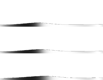
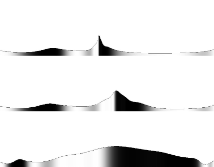
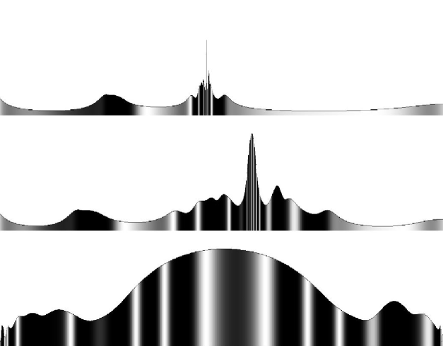
Figure 1: Time evolution of the distribution of the inflaton scalar field $\phi$, shown by the upper boundary of the shaded area, and the scalar field $\Phi$, shown by the color (black – white). This distribution is shown as a function of one coordinate $x$, in a domain of initial size $H^{-1}(\phi_{0})$. We present a sequence of three panels for each time $t$. The first one shows the distribution of the fields in the comoving coordinates, which is related to the probability distribution $P_{c}$. The second one exhibits the same fields in the coordinates which show the physical distance from one point to another, divided by the total distance between the two sides of the domain. The third one shows the distribution of the fields per unit physical three-dimensional volume, which would correspond to the distribution $P_{p}$ in a three-dimensional Universe.

The second panel shows the same distribution of the scalar field, but in different coordinates, which take into account different rate of expansion in different domains. To achieve this goal, at each step $\Delta t$ of our calculations we expand the distance between the nearby points by $e^{H(\phi(x,t))\Delta t}$. After that, the computer displays the resulting distribution at the interval of the original size, as if there were no change in the total length of the domain. The distribution of the field $\phi$ in these figures corresponds to the probability distribution $P_{p}$, and the squeezing of the interval back to its original size automatically normalizes this distribution. This means that the distribution of the scalar field shown at the lower figure gives a good idea of the relative fraction of volume of the Universe filled by the field $\phi$.

Well, this is not quite correct. These figures give a good idea of the relative fraction of length of a one-dimensional Universe filled by the field $\phi$. Indeed, our computer simulations here were one-dimensional. To get a correct idea of how the probability distribution $P_{p}$ behaves in a three-dimensional Universe, each time $\Delta t$ one should expand the distance between the points by $e^{3H(\phi(x,t))\Delta t}$. This gives a distorted spatial distribution of the scalar field, but this distribution shows in a correct way the distribution of the three-dimensional volume of the Universe filled by the field $\phi$. This is shown at the third panel (the third series of figures in Fig. 1, the lowest ones).

Black and white regions in these figures correspond to the distribution of another scalar field, which we added to our model. This is a scalar field $\Phi$ with the effective potential $V(\Phi)$ which may have several different minima. It is assumed that during the stage of inflation driven by the field $\phi$, the effective potential $V(\Phi)$ is much smaller than $V(\phi)$. Therefore, at this stage one may neglect the contribution of the field $\Phi$ to the rate of expansion of the Universe. However, this field may be responsible for the symmetry breaking in the theory of elementary particles. The field $\Phi$ also experiences quantum fluctuations and Brownian motion.

This Brownian motion can push the field $\Phi$ from one minimum of $V(\Phi)$ to another. Then, after the end of inflation, the field $\Phi$ becomes trapped by the minimum to which it jumped, and it cannot move from it anymore. However, in different exponentially large domains of the Universe this field may be trapped in different minima. As a result, the Universe becomes divided into exponentially large domains with different types of elementary particle physics inside each of them.

To give a particular example of such theory, we will consider a model with the effective potential

$$V(\Phi)=V_{0}~{}\left(1-\cos{N\Phi\over\Phi_{0}}\right)~{},$$ (79)

where $N$ is some integer. The ratio $\Phi\over\Phi_{0}$ is considered as an angular variable. Such potentials appear, e.g., in the theory of the axion field, as well as in the model of ‘natural inflation’ driven by the field $\Phi$. The amplitude of the quantum jumps of the field $\Phi$ is described by the same equation (76) as for the field $\phi$; to study the classical motion of the field $\Phi$ one should apply eq. (78) to this field.

In our series of computer simulations of the one-dimensional inflationary Universe, we take a particular value $N=2$. In this case the effective potential (79) has two minima of equal depth, $V(\pi\Phi_{0})=V(-\pi\Phi_{0})=0$. We use black color to show the parts of the Universe with $\Phi\sim\pi\Phi_{0}$, we use white color to show the parts with $\Phi\sim-\pi\Phi_{0}$, and we use various shades of grey to show intermediate regions.

Our calculations begin with a domain of initial size $H_{0}^{-1}$ filled by some homogeneous (or almost homogeneous) fields $\phi$ and $\Phi$. After few steps the distribution of the scalar field $\phi$ becomes slightly inhomogeneous. At the same time the inhomogeneities generated in the field $\Phi$ may be relatively large, if their amplitude $\delta\Phi\sim\sqrt{u}H$ is large in comparison with $\Phi_{0}$. As a result, the field $\Phi$ rapidly jumps from one minimum of its effective potential to another, and the Universe becomes divided into approximately equal number of black and white regions.

After few steps of calculation the scalar field $\phi$ also becomes very inhomogeneous. However, this inhomogeneity looks different on the three different series of figures we produced. In comoving coordinates (upper figures) the field $\phi$ in the most part of space decreases; we see only few hills, which in the course of time grow and produce many thin spikes. However, in the physical coordinates, which take into account exponential expansion of the Universe, these thin spikes look like large mountains, see figures in the middle. Gradually these mountains occupy more and more space, and their physical size grows exponentially. Also, these mountains are never sharp; they are build from the sinusoidal waves which always look very smooth on the scale $H^{-1}$. (The two last statements are only partially illustrated by the figures, since the mountains look more narrow than they really are after the computer shrinks the expanded interval back to its original size.)

Finally, the last series of figures shows a very rapid growth of the relative fraction of volume of the Universe occupied by the growing field $\phi$. This exactly corresponds to the process of self-reproduction of the Universe. We see also that quantum fluctuations of the scalar field $\Phi$ lead to formation of exponentially large number of black and white domains, corresponding to different types of symmetry breaking in the theory (79).

IV.2 One-dimensional Universe in the $\tau$-parametrization of time

Similar calculations can be done for the $\tau$-parametrization of time, where $\tau=\ln{{a\left(x,t\right)\over a(x,0)}}$. This immediately reveals an important difference between this parametrization of time and the standard one. First of all, now all three sets of figures look absolutely the same, since, by definition, at a given time $\tau$ the degree of exponential expansion is the same for all points $x$. An important difference between the corresponding distributions $P_{c}$ and $P_{p}$ is that the distribution $P_{c}$ is not stationary: the comoving volume of the regions filled by the large field $\phi$ decreases. Meanwhile, the total volume of the domains filled by the large field $\phi$, which is given by $P_{p}$, increases exponentially. As we will show in this paper, after we divide $P_{p}$ by the overall growth of the volume of the Universe, we obtain a stationary normalized distribution $\tilde{P}_{p}$.

Unfortunately, this difference between $P_{c}$ and $P_{p}$ cannot be seen in our figures. Therefore we will present only one figure (Fig. 2) instead of the three series of figures. This figure shows the distribution of the scalar fields $\phi$ and $\Phi$ after a few steps of our computer simulations. It illustrates a specific difference between the distributions at a given $t$ and at a given $\tau$. The typical wavelength of inhomogeneities of the field $\phi$ in the $\tau$-parametrization of time is approximately constant in different parts of the Universe, whereas the field $\phi$ in the $t$-parametrization is much more inhomogeneous near the maxima of its distribution in comoving coordinates.

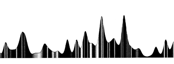
Figure 2: The distribution of the fields $\phi$ and $\Phi$ after several steps in time $\tau$.

From the technical point of view, the difference between the two calculations is reflected in the equations for the perturbations $\delta\phi$ and $\delta\Phi$, and for their classical shift during the time interval $\Delta t=u$ corresponding to one step of our calculations. For example, for the field $\phi$ we have

$$\delta\phi(x,y)={H(\phi(x))\sqrt{u}\over\sqrt{2}\pi}\cdot\sin\Bigl{(}H(\phi(x))~{}e^{\tau}\,x+\alpha_{n}\Bigr{)}~{},$$ (80)

and

$$\Delta\phi(x,y)=-\,{uV^{\prime}(\phi)\over 3H^{2}(\phi(x,t))}\ \,.$$ (81)

IV.3 Fluctuations in a two-dimensional Universe

When generalizing our methods for two- or three-dimensional Universe in time $t$, one meets several complications. First of all, it is possible to plot the distribution of the field in comoving coordinates, but it is very difficult to stretch these coordinates to show the distribution of the fields per unit physical volume, as we did for the one-dimensional Universe. This seems to be a rather general problem, since it is not always possible to show the curvature of space by representing it as a curved surface in a flat space of higher dimension. Therefore we represented all our results in the comoving coordinates only.

Another problem is related to the possibility to represent quantum fluctuations of the scalar field by plane waves. In one-dimensional Universe this was an easy problem, but in a two dimensional curved Universe this is impossible. In some sense, the waves of the scalar field look as if they were propagating in a medium with an exponentially large refraction coefficient. This refraction coefficient changes from point to point. If one starts with a plane wave at some point $x$, it does not remain a plane wave at some distance from this point: the front of the wave becomes strongly bent because of gravitational lensing.

This is not a real problem if one studies only relatively small domains, but even if one starts with a very small domain, eventually its size becomes exponentially large, and the effects of bending become more and more significant. Therefore, if one wishes to investigate evolution of the scalar field in the whole domain, one should find some other way to simulate quantum fluctuations of the scalar field, which would lead to the same (or almost the same) correlation functions (19)-(22) as the ordinary plane wave fluctuations, while being free from the problems mentioned above. Such a method does exist: one should use functions $\delta\phi(x)$ which look like plane waves inside domains of a sufficiently large radius $r_{0}$, where $r_{0}\gg H^{-1}$. However, these functions should rapidly decrease at $r>r_{0}$. Such functions are called wavelets David .

A simplest example of a wavelet which we used in our calculations looks as follows:

$$\delta\phi(x,t)=a\,\exp\left(-C^{2}({\bf r}-{\bf r}_{n})^{2}\cdot H^{2}({\bf r}_{n},t))\right)\times\,\sin\left(H({\bf r}_{n},t)){\lambda_{p}({\bf r}_{n},t)\over\lambda_{c}({\bf r}_{n},t)}(x\sin\theta_{n}+y\cos\theta_{n}+\alpha_{n})\right)~{}.$$ (82)

Here $a={H(\phi({\bf r}_{n},t))\over\sqrt{2}\pi}\,{\sqrt{uH(\phi({\bf r}_{n},t))\over H(\phi_{0})}}$,  $\theta_{n}$ and $\alpha_{n}$ are random numbers, $C$ is some constant, $({\bf r}-{\bf r}_{n})^{2}$ is the square of the physical distance from the center of the wavelet ${\bf r_{n}}$ to the point ${\bf r}$. In the comoving coordinates $x$ and $y$

$$({\bf r}-{\bf r}_{n})^{2}=\Bigl{(}(x-x_{n})^{2}+(y-y_{n})^{2}\Bigr{)}\cdot{\lambda^{2}_{p}({\bf r}_{n},t)\over\lambda^{2}_{c}({\bf r}_{n},t)}\ .$$ (83)

At $C\ll 1$ this field configuration looks like a sinusoidal wave with an amplitude which is given by $a$ at ${\bf r}={\bf r_{n}}$, and which becomes exponentially small at a distance about $(CH)^{-1}$ from the center of the wavelet. In the limit $C\to 0$ wavelets would behave as ordinary plane waves. Thus, one should take $C$ small, but not too small, to avoid the effect of gravitational lensing inside the wavelets.

The procedure of simulation of quantum perturbations of the scalar field consisted of generation of a proper number density of wavelets and of their distribution at random points ${\bf r_{n}}$ in such a way that the number of the wavelets in a given domain is proportional to its physical volume (i.e. to $e^{\int 3H({\bf r}_{n},t)\,dt}$). By choosing a proper number density of wavelets we mean that the variance of perturbations produced by wavelets in the limit when the Universe is homogeneous should coincide with the standard result $<(\delta\phi)^{2}>=H^{3}t/4\pi^{2}$.

Our choice of the form of the wavelets is not perfect, but it is good enough for our purposes. Ideally, one should consider wavelets which form a complete orthonormal set of functions, like it is done in the usual Fourier analysis. It is well known that the wavelet transform can give a much better information about very inhomogeneous structures than the standard Fourier transform David . It is also known that the usual momentum representation, which is related to the Fourier transform, is not suitable for formulation of quantum field theory in curved space. We were forced to use wavelets instead of plane waves to perform a consistent computer simulation of quantum fluctuations in the usual $t$-parametrization of time. This gives us a hint that the wavelet transform, rather than the standard Fourier transform, may become a very useful tool for field quantization in curved space.

On the other hand, in some simple but important cases one may escape from the difficulties associated with gravitational lensing by choosing a different set of coordinates. In our case everything becomes very simple in the $\tau$-parametrization of time, where $\tau\sim\log a(t)$. Computer simulations of the evolution in time $\tau$ are much easier SB . In particular, one can use ordinary plane waves, but with the amplitude proportional to ${H(\phi({\bf r}_{n}))\sqrt{u}\over\pi\sqrt{2}}$. The reason is that different parts of inflationary Universe expand by the same number of $e$-foldings at a given value of the time $\tau$. From the point of view of computer simulations this means that expansion of the Universe does not introduce any distortions into the original grid of comoving coordinates $x$ and $y$. However, it would be incorrect to make computer simulations in time $\tau$ instead of simulations in time $t$. These two approaches are complimentary to each other, emphasizing different features of the same process. For example, as we have already seen in our study of one-dimensional Universe, sometimes it is easier to illustrate the process of self-reproduction of inflationary domains using ordinary $t$-parametrization of time. Figures 3–6 contained in this section were obtained by computer simulations of the evolution of scalar fields in time $t$, whereas Fig. 7 corresponds to the time $\tau$.

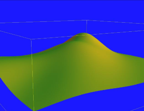
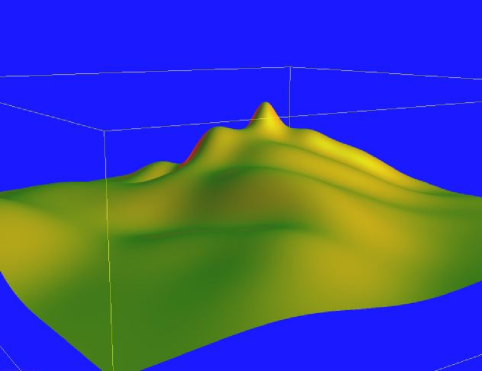
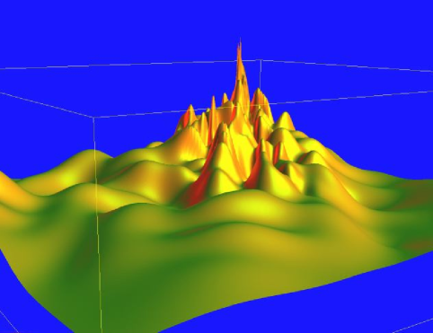
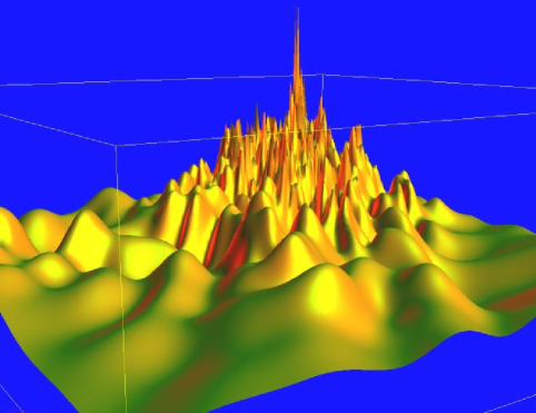
Figure 3: The evolution of the scalar field $\phi$ in a two-dimensional inflationary Universe in time $t$.

The set of Figs. 3 shows the evolution of the scalar field in time $t$. We begin our simulations with an almost homogeneous scalar field $\phi\sim\phi_{0}$ inside a domain of initial size $H^{-1}(\phi_{0})$, which is represented by a grid containing $1000\times 1000$ points, Fig. 3.1. Then the Universe expands, the amplitude of the classical scalar field slowly decreases, but due to overlapping of waves (=wavelets) corresponding to fluctuations of the scalar field, the amplitude of the scalar field in some parts of the expanding domain becomes much greater than $\phi_{0}$. This corresponds to growing mountains on Figs. 3.2–3.6. We should emphasize again that the peaks of these mountains are not sharp at all; they are built from fluctuations with the physical wavelength $\sim H^{-1}$. They look sharp since we are plotting everything in comoving coordinates, in which the wavelength of perturbations $\lambda_{c}$ becomes exponentially small, especially in the parts of the Universe where $\phi$ is large and expansion is fast (i.e. on the tops of the mountains).

In the parts of the Universe where the scalar field becomes small there are no high mountains; the field continues moving towards $\phi=0$. We live in one of such parts of the Universe. The perturbations of the scalar field generated at this stage of inflation are relatively small. These perturbations are responsible for the small perturbations of temperature of the microwave background radiation discovered by COBE.

However, if $\phi_{0}$ is greater than some critical value $\phi^{*}$, then mountains with $\phi>\phi^{*}$ are permanently produced. This corresponds to the process of the Universe self-reproduction. The effective potential of the field $\phi$ on tops of some of these mountains becomes greater than the Planck density. (In these simulations we did not introduce any boundary conditions at the Planck density; see however the next Section.) One may envisage each of such tops as a beginning of a new “Big Bang”. If one wishes to reserve this name for the first “Big Bang” (if there was one), one may think about such names as a “Small Bang” or “Pretty Big Bang”. Whatever the words, the theory we have now is considerably different from the old Big Bang theory.

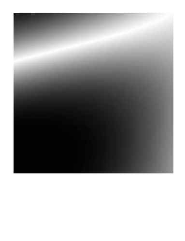
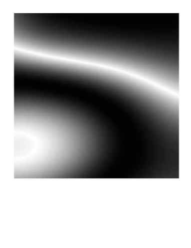
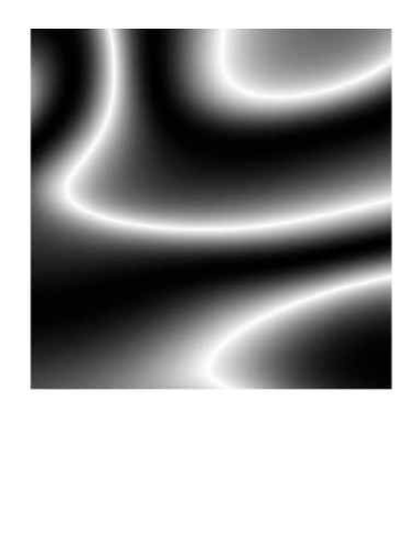
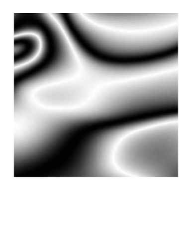
Figure 4: Generation of axion domain walls during inflation.

The series of Figures 4 corresponds to a more complicated theory of elementary particles, which includes another scalar field, $\Phi$, with the effective potential (79) with $N=1$. In this case the shape of the effective potential $V(\Phi)$ coincides with the shape of the effective potential in the simplest version of the axion theory. In these figures we do not show the evolution of the inflaton scalar field $\phi$; thus, no mountains. We just show the distribution of the fluctuating scalar field $\Phi$ on the plane $(x,y)$. White regions correspond to the minima of $V(\Phi)$ at $\Phi/\Phi_{0}=2n\pi$, black regions correspond to the maxima at $\Phi/\Phi_{0}=(2n+1)\pi$.

In the beginning of our calculations the color (the level of grey) only slowly varies in the domain of initial size $\sim H^{-1}$, Fig. 4.1. Later on, in the main part of the domain (in comoving coordinates) the field $\Phi$ moves towards the minima of its effective potential, but in some places the field diffuses, say, from the minimum at $\Phi/\Phi_{0}=0$ to the minimum at $\Phi/\Phi_{0}=2\pi$. On the way it passes through the maximum at $\Phi/\Phi_{0}=\pi$, and in some places the field stays at this maximum, forming a domain wall between the domains with $\Phi/\Phi_{0}=0$ and with $\Phi/\Phi_{0}=2\pi$. The existence of such domain walls in the axion theory was first pointed out by Sikivie Sik . The inflationary mechanism of their production described above was discussed in LinLyth . The series of Figures 4 shows the process of formation of these domain walls, which look as thin black lines at Fig. 4.

Figure 5: Axion domain walls in a model with a smaller value of $\Phi_{0}$ (Pollock Universe).

The distribution and the properties of domain walls in the axion theory are very sensitive to the values of parameters of the theory. For example, by reducing the radius $\Phi_{0}$ of the effective potential (79) one obtains much more domain walls per unit volume, see Fig. 5. For obvious reasons, we called this figure ‘Pollock Universe’.

Now let us consider the same model, but with $N=2$, as we did in our one-dimensional calculations. In this case in the interval $0<\Phi/\Phi_{0}<2\pi$ we have two different minima with $V=0$. From the point of view of perturbations produced during inflation, there is no much difference between the cases $N=1$ and $N=2$; domain structure will be generated in each case. But now we assume that some properties of particles interacting with the field $\Phi$ change when the field $\Phi/\Phi_{0}$ jumps from one minimum to another. This happens, for example, in the supersymmetric $SU(5)$ model, where there exist many minima of the same depth corresponding to different types of symmetry breaking in the theory. To distinguish between the minima at $\Phi/\Phi_{0}=2n\pi$ and the minima at $\Phi/\Phi_{0}=(2n+1)\pi$ we will paint the first ones white and the second ones black, just as we did in our one-dimensional calculations.

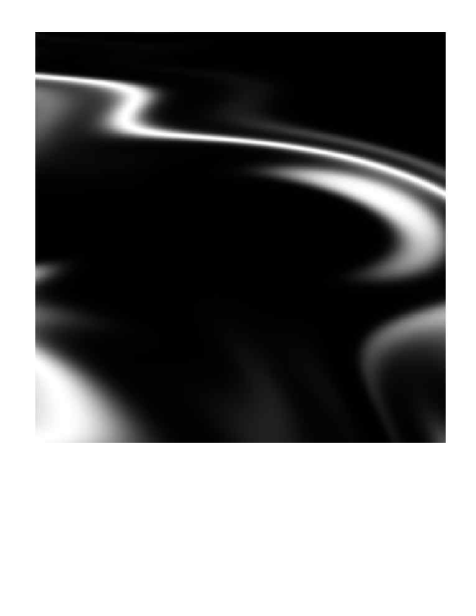
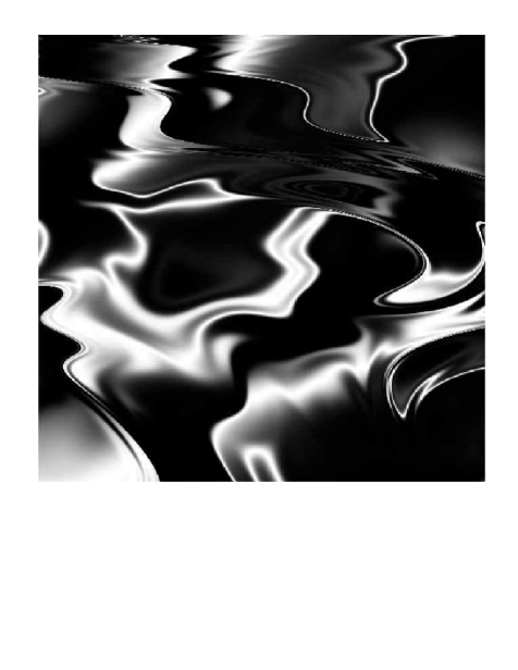
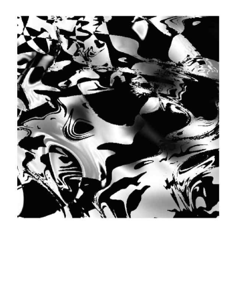
Figure 6: Generation of domain structure of the Universe during inflation in the axion model with $N=2$ (Kandinsky Universe).

The results of the calculations are represented by a series of Figures 6. Originally the whole initial domain contains the scalar field in one of the minima of its effective potentials. Then this field begins jumping from one minimum to another, and the Universe becomes divided into many exponentially large black and white domains. Figures 6 show that in the course of time the domain which originally was quite homogeneous becomes looking like a huge fractal. We called this fractal ‘Kandinsky Universe’.

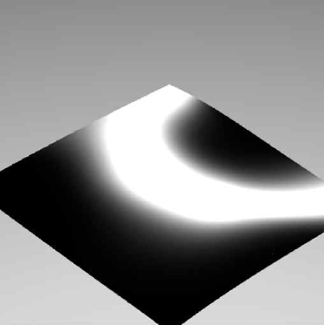
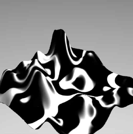
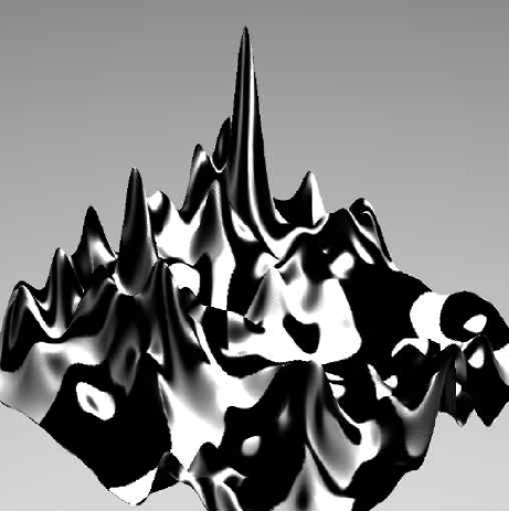
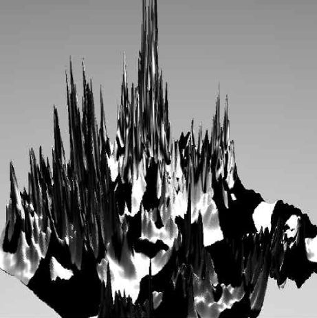
Figure 7: The distribution of the scalar fields $\phi$ and $\Phi$ in a two-dimensional Universe after several steps in time $\tau$.

In Figs. 7, which we obtained by studying the of stochastic processes in the time $\tau$, we plot simultaneously the distribution of the inflaton field $\phi$ and of the field $\Phi$. By looking at these figures one can find that the most chaotic and rapidly changing distribution of black and white domains corresponds to the regions near the peaks of the distribution of the field $\phi$. In these regions the color of the domains changes very rapidly, which means that the laws of the low-energy elementary particle physics (which are related to the type of spontaneous symmetry breaking) are not fixed there yet. However, in the valleys, where the inflaton field $\phi$ is small, the color becomes fixed. We live in one of such domains of a given color. Other domains are exponentially far away from us. And there are domain walls separating domains with different colors. Laws of low energy physics change as one jumps through the domain walls; one should think twice before doing so.

An interesting feature of all these computer simulations is the following. If one takes a magnifying glass and looks at some part of the picture of a physical size of the order of $H^{-1}$, one will see a rather homogeneous distribution of the scalar fields $\phi$ and $\Phi$. Then one may start computer simulations again. And again one will get mountains of the same type, and a Universe consisting of domains of different colors. This is the first (and the most fundamental) kind of stationarity which we certainly have in our Universe. Not only the Universe looks like a fractal at any given moment of time, it actually is a growing fractal, which reproduces itself over and over again.

As we already mentioned, the fractal structure of the inflationary Universe in the theories where inflation occurs near a local maximum of effective potential $V(\phi)$ is relatively simple; one can easily calculate the fractal dimension of the inflationary Universe ArVil . The corresponding structure in the chaotic inflation scenario with $V(\phi)\sim\phi^{n}$ or with $V(\phi)\sim e^{\alpha\phi}$ is much more complicated, but it is also much more interesting. From the point of view of computer simulations, the fractal structure of the Universe in this scenario has more “colors” in it, since quantum fluctuations near the Planck density allow more profound changes of the vacuum state.

V Towards the Theory of a Stationary Universe

V.1 Are there Any Stationary Solutions for $P_{p}$?

Now let us return to the problem of stationarity of the distribution $P_{p}(\phi,t)$. Eq. (66) suggests that there are no stationary distributions not only for $P_{c}$, but for $P_{p}$ as well. This conclusion, however, may fail when the field $\phi$ approaches $\phi_{p}$ and density approaches the Planck density $\rho_{p}\sim M^{4}_{p}=1$. One of the reasons is that at $\rho\mathrel{\hbox{\hbox to0.0pt{\hbox{\lower 4.0pt\hbox{$\sim$}}\hss}\hbox{$>$}}}1$ the probability distribution $P_{c}$ becomes strongly non-Gaussian, dispersion of fluctuations of the field $\phi$ becomes very large and our derivation of eq. (66) does not work. To avoid this problem, one may try to find exact solutions of eq. (65).

An attempt to do this was made in very important papers by Nambu and Sasaki Nambu . It was claimed that in theories $V(\phi)\sim\phi^{n}$ with $n<4$ the distribution $P_{p}$ is always nonstationary, but in theories with steeper effective potentials ($V(\phi)\sim\phi^{n}$ with $n\geq 4$, or $V(\phi)\sim e^{c\phi}$) stationary distributions for $P_{p}$ do exist. However, the stationary distributions which were found in Nambu have their maxima at densities $\rho\gg\rho_{p}=1$. These results are unreliable for several different reasons:

1. Eq. (55) may have a slightly different form, which corresponds to the difference between possible definitions of stochastic term in the equation (48). This difference is not important at densities much smaller than $1$, but at $\rho\mathrel{\hbox{\hbox to0.0pt{\hbox{\lower 4.0pt\hbox{$\sim$}}\hss}\hbox{$>$}}}1$ it may become significant. (Note, however, that this is not an unsolvable problem. One may just investigate modified equations as well. Two other problems are more fundamental.)

2. Diffusion equations were derived in the semiclassical approximation which breaks down near the Planck energy density.

3. Interpretation of the processes described by these equations is based on the notion of classical fields in a classical space-time, which is not applicable at densities greater than $1$ because of large fluctuations of metric at such densities. In particular, our interpretation of $P_{c}$ and $P_{p}$ as of probabilities to find classical field $\phi$ at a given point (or in a given volume) at a given time does not make much sense at $\rho>1$.

Thus, the results of ref. Nambu do not help us to establish the existence of stationary solutions. However, it is obvious that there exists a class of theories where $P_{p}$ is stationary even though $V(\phi)$ grows indefinitely at large $\phi$. For example, one can consider a theory with the effective potential $\sim\lambda\phi^{n}\exp\Bigl{(}{\phi\over C\phi^{*}}\Bigr{)}^{2}$, with $C\gg 1$. (Similar effective potentials often appear in supergravity.) In such a theory we have both inflation and self-reproduction of the Universe. However, at $\phi>C\phi^{*}$ inflation is impossible since the potential is too steep. Therefore the distribution $P_{p}$ will be unable to move to $\phi>C\phi^{*}$, and will become stationary.

There is another, more general reason to expect the existence of stationary solutions. As we will argue now, inflation tends to kill itself as the energy density approaches the Planck density.

In our previous investigation we assumed that the vacuum energy density is given by $V(\phi)$ and the energy-momentum tensor is given by $V(\phi)\,g_{\mu\nu}$. However, quantum fluctuations of the scalar field give the contribution to the average value of the energy momentum tensor, which does not depend on mass (for $m^{2}\ll H^{2}$) and is given by b99

$$<T_{\mu\nu}>\,=\,{3\,H^{4}\over 32\,\pi^{2}}\ g_{\mu\nu}\,=\,{2\over 3}\,V^{2}\ g_{\mu\nu}\ .$$ (84)

One of the sources of this contribution is obvious. Quantum fluctuations of the scalar field $\phi$ freeze out with the amplitude ${H\over 2\pi}$ and the wavelength $\sim H^{-1}$. Thus, they lead to the gradient energy density $(\partial_{\mu}\delta\phi)^{2}\sim H^{4}$.

Note, that eq. (84) does not give the total contribution of quantum fluctuations to the energy density. When the field $\phi$ is outside the minimum of the effective potential, additional terms appear, in particular, the term $\sim V^{\prime}(\phi)\delta\phi$ (23) which is responsible for galaxy formation. At $\phi<\phi^{*}$, when the density perturbations responsible for galaxy formation were produced, the vacuum energy renormalization (84) is subdominant. On the other hand, at $\phi>\phi^{*}$ the contribution corresponding to eq. (84) becomes greater than $V^{\prime}(\phi)\delta\phi\sim V^{\prime}(\phi)H/2\pi$. For example, in the theory $V=m^{2}\phi^{2}/2$

$${2\,V^{2}\over 3}\,=\,{m^{4}\phi^{4}\over 6}\,\mathrel{\hbox{\hbox to0.0pt{\hbox{\lower 4.0pt\hbox{$\sim$}}\hss}\hbox{$>$}}}\,{V^{\prime}(\phi)H\over 2\pi}=2m^{3}\phi^{2}\sqrt{\pi\over 3}\$$ (85)

for $\phi\mathrel{\hbox{\hbox to0.0pt{\hbox{\lower 4.0pt\hbox{$\sim$}}\hss}\hbox{$>$}}}\phi^{*}\sim 1/\sqrt{m}$.

An interesting property of eq. (84) is that the average value of the energy-momentum tensor of quantum fluctuations does not look like an energy-momentum tensor corresponding to the gradients of a sinusoidal wave. It looks rather like a renormalization of the vacuum energy-momentum tensor (it is proportional to $g_{\mu\nu}$). This result appears after averaging over all short-wavelength fluctuations and over all possible outcomes of the process of generation of long-wavelength perturbations. Something similar happens when one calculates the energy-momentum tensor in ordinary flat space-time: the contribution of each wave is not proportional to $g_{\mu\nu}$, but the energy-momentum tensor becomes proportional to $g_{\mu\nu}$ after integration over all such contributions with the invariant measure $\sim\delta(k^{2}-m^{2})$. However, if we are not integrating over all long-wavelength perturbations, but treat them as a classical inhomogeneous scalar field, then at each particular time interval $\sim H^{-1}$ in each particular $h$-region the energy momentum tensor of these perturbations is mainly due to the gradient energy density $(\partial_{\mu}\delta\phi)^{2}$, and it is not proportional to $g_{\mu\nu}$.

This does not lead to any interesting effects at $V\ll 1$ ($\phi\ll\phi_{p}$) since in this case $V^{2}\ll V$. However, at the density comparable with the Planck density the situation becomes much more complicated. At $V>1$ the gradient energy density $\sim V^{2}$ becomes greater than the potential energy density $V(\phi)$. A typical wavelength of perturbations giving the main contribution to the gradient energy is given by the size of the horizon, $l\sim H^{-1}$. This means that the inflationary Universe at the Planck density becomes divided into many domains of the size of the horizon, density contrast between these domains being of the order of one. These domains evolve as separate mini-Universes with the energy density dominated not by the potential energy density but by the energy density of gradients of the field $\phi$. Such domains drop out from the process of exponential expansion. Some of them may reenter this process later, but many of them collapse into black holes within the typical time $H^{-1}$ and then evaporate. Indeed, the standard criterion for the formation of primordial black holes is exactly the requirement that the local increase of density $\delta\rho$ is comparable to $\rho$ on the scale of the horizon. This criterion is satisfied for perturbations of density produced at $V(\phi)\mathrel{\hbox{\hbox to0.0pt{\hbox{\lower 4.0pt\hbox{$\sim$}}\hss}\hbox{$>$}}}1$.

Of course, one may argue that all our considerations do not make sense at densities greater than the Planck density. When the energy density in any $h$-region approaches the Planck density, it may no longer be described in terms of classical space-time and should be just thrown away from our consideration. In particular, its volume should not be considered as contributing to the total volume of the Universe. Thus, such domains should be neglected in our definition of $P_{p}$. In this case the distribution $P_{p}$ for the field $\phi$ will stop growing and will approach a stationary regime when this distribution will be shifted towards $\phi\sim\phi_{p}$.

We are making an even stronger statement. Even if one makes an attempt to consider the domains with $V>1$ as a part of classical space-time, many such domains drop out from the process of inflation. This means that the total volume of inflationary $h$-regions cannot grow as fast as $e^{3H(\phi)t}$ for $\phi>\phi_{p}$.

In the models describing many different scalar fields inflation may become self-destructing even at an energy density somewhat smaller than the Planck density. Let us consider, for example, an inflationary model describing $N$ different scalar fields, with $N\gg 1$. The Hubble constant in such a theory is determined by the sum of all effective potentials, $V=V_{1}+V_{2}+...$. The Planck density can be defined as a density at which all higher order gravitational corrections are equally important. The one-loop correction to the energy-momentum tensor (84) in our model is directly proportional to the number of scalar fields $N$, but the second-loop corrections do not contain such an enhancement. Thus, one may argue that the Planck density in our model remains the same, $\rho_{p}\sim 1$. On the other hand, the energy density of gradients of the scalar field fluctuations now is proportional to $N$:

$$(\partial_{\mu}\delta\phi)^{2}\,\sim\,N\,V^{2}\ .$$ (86)

This means that the gradient energy density becomes greater than the potential energy density $V$ at $V\sim{1\over N}\ll 1$. In the model with large $N$ this does not automatically imply black hole formation, since density perturbations will be suppressed by $1/\sqrt{N}$. However, if the energy density of any domain of a size $l\mathrel{\hbox{\hbox to0.0pt{\hbox{\lower 4.0pt\hbox{$\sim$}}\hss}\hbox{$>$}}}H^{-1}$ becomes dominated by the gradient energy, such a domain instead of inflation enters the regime of a slow power-law expansion. At this stage, previously generated fluctuations of the scalar fields either oscillate or at least considerably decrease. This breaks down the standard scenario of the new scalar field fluctuations freezing out on the top of the previously frozen fluctuations.

In fact, some predecessors of self-destruction of inflation show up already at sub-Planckian densities even at small $N$. When we discussed the derivation of the diffusion equation for $P_{c}$, we assumed that all  perturbations of the wavelength $H^{-1}$ give rise to inflationary domains. However, this is not the case for very large fluctuations of the field $\phi$ with the amplitude of a fluctuation $\delta\phi>1$. Such fluctuations should be present if, as we assumed, the term $\xi(t)$ in the Langevin equation (48) corresponds to the white noise. The gradient energy of the perturbations of the wavelength $H^{-1}$ with the amplitude $\delta\phi>1$ is given by ${1\over 2}\,(\partial_{\mu}\delta\phi)^{2}>H^{2}\sim V(\phi)$. Domains where such jumps occur may drop out of the process of exponential expansion. Suppression of inflation in the domains of a size $H^{-1}$ produced by large jumps effectively implies that the effective noise in the Langevin equation is not entirely white.

The probability of such a large jump within the time $H^{-1}$ is suppressed by $\exp\left(-{2\pi^{2}\delta\phi^{2}\over H^{2}}\right)$. This indicates that at $H\ll 1$ (i.e. at sub-Planckian densities) the cut-off of noise corresponding to fluctuations with the amplitude $\delta\phi\mathrel{\hbox{\hbox to0.0pt{\hbox{\lower 4.0pt\hbox{$\sim$}}\hss}\hbox{$>$}}}1$ is not very important, since the probability of such fluctuations is exponentially suppressed. However, the closer we are to the Planck density, the stronger is the deviation of $\xi(t)$ from the white noise, the less efficient is the stochastic process producing new inflationary domains.

What are the possible consequences of this effect? First of all, we know that if the initial value of the field $\phi$ is in the interval $\phi^{*}<\phi<\phi_{p}$, then the distribution $P_{p}(\phi,t)$ moves towards greater and greater $\phi$. The only reason why it happens, despite the fact that the distribution $P_{c}(\phi,t)$ moves towards small $\phi$, is an additional exponential growth of the number of inflationary $h$-regions due to expansion of the Universe. If, as we argued, the number of inflationary $h$-regions with $\phi\sim\phi_{p}$ grows at a much slower rate (or does not grow at all, which is the case if we just do not consider domains with $\phi>\phi_{p}$ as belonging to our classical space-time), then the distribution $P_{p}(\phi,t)$ stops moving towards large $\phi$ as soon as the maximum of this distribution approaches $\phi_{p}$. Thus, the distribution $P_{p}(\phi,t)$ may approach some stationary regime, being concentrated at sub-Planckian densities. Now let us study this possibility at a more quantitative level.

V.2 Self-Reproduction of Inflationary Domains as a Branching Diffusion Process

When describing the process of self-reproduction of inflationary domains one should keep in mind that this is not an ordinary diffusion process, but process where diffusion of the scalar field in each particular $h$-region is accompanied with their branching into many independent $h$-regions. As was argued in MezhMolch , a good candidate for the mathematical model describing such behavior is the theory of branching diffusion processes Watanabe .

There are two main sets of questions which may be asked concerning such processes. First of all, one may be interested in the probability $P_{p}(\phi,t|\phi_{0})$ to find a given field $\phi$ at a given time $t$ under the condition that initial value of the field was equal to some $\phi_{0}=\phi(t=0)$. In what follows we will denote $\phi_{0}$ as $\chi$.

On the other hand, one may wish to know, what is the probability $P_{p}(\phi,t|\chi)$ that the given final value of the field $\phi$ appeared as a process of diffusion and branching of a domain containing some field $\chi$. Or, more generally, what are the typical properties of branching Brownian trajectories which end up at a hypersurface of a given $\phi$?

In the end of the Section III.2 we have shown that the probability to find a given field $\phi$ in a given volume moves towards Planckian densities with the growth of time $t$, if $\phi_{0}>\phi^{*}$. We have shown also that a typical trajectory producing domains of a given density for a long time fluctuates at very large $\phi$, close to the Planck density. Thus, we obtained qualitative answers for the two questions mentioned above. To obtain a more quantitative description of the process of self-reproduction of the Universe, we will first develop more general methods of investigation using the simplest characteristics of the branching diffusion processes which involve only those parameters of the model MezhMolch that can be unambiguously identified at this stage of our studies.

Many properties of a branching diffusion process can be reproduced with the help of the following function

$$u(\chi,t,{\cal D})\,=\ \left\langle\left.{\mu(t,{\cal D})}\right|\,\phi_{0}=\chi\right\rangle\ .$$ (87)

Here $\mu(t,{\cal D})$ is the number of “particles” with the coordinates $x$ in the interval   ${\cal D}$ at the moment   $t$. In our case the analog of a particle with a coordinate $x$ is the $h$-region with a given field $\phi$. The interval of all possible values of $\phi$ corresponding to inflation in classical space-time is ${\cal D}_{max}=[\phi_{e},\phi_{p}]$. However, one may choose to consider as ${\cal D}$ in eq. (87) any smaller segment of the interval $[\phi_{e},\phi_{p}]$.

By $\left\langle\left.{\mu(t,{\cal D})}\right|\,\phi_{0}=\chi\right\rangle$ we denoted the mathematical expectation value (or, in other words, the mean value) of the number of “particles” in the interval ${\cal D}$ at the moment $t$ under the condition that initially there was one “particle” with $\phi_{0}=\chi$.

The last condition implies that

$$u(\chi,0,{\cal D})=\left\{\begin{array}[]{ll}1,&\mbox{if $\chi\in{\cal D}$}\ ,\\ 0,&\mbox{otherwise}\ .\end{array}\right.$$ (88)

There is some subtlety in definition of the ‘number of particles’ $\mu(t,{\cal D})$ in the stochastic approach to inflation. Depending on the way one formulates the problem, this may be either the number  ${\cal N}(t,{\cal D})$ of $h$-regions or their total volume  ${\cal V}(t,{\cal D})$ divided by some normalization factor $H^{-3}(\phi_{0})$. The difference between these two quantities stems from the fact that the total volume of each $h$-region is proportional to $H^{-3}(\phi)$, where $\phi$ is the local value of the scalar field in a given $h$-region. This difference typically is not very important: it is proportional to the third power of ${H(\phi)\over H(\phi_{0})}$, whereas most of the distributions we will obtain depend on $H(\phi)$ exponentially. Nevertheless, whenever appropriate, we will make a distinction between these two understandings of $\mu(t,{\cal D})$. In what follows, we will understand by $\mu(t,{\cal D})$ the volume ${\cal V}(t,{\cal D})$ of the $h$-regions with the scalar field $\phi\in{\cal D}$. (For an equation describing the number of $h$-regions ${\cal N}$ see also Mijic ).

Now we will try to find an equation describing the time evolution of $u(\chi,t,{\cal D})$. The space-time structure of the branching diffusion process may be represented by a growing tree of world lines of diffusing particles. The section of the tree at some level represents the spatial distribution of the particles at the corresponding moment of time, while the increasing number of “branches” corresponds to the increasing number of particles due to the processes of “splitting” of one “parent” particle into several “daughter” ones. Here we produce a derivation of the reduced form of the equation describing the growth of this tree MezhMolch in a way which does not involve any new model parameters in addition to those already presenting in the chaotic inflation.

Consider the whole tree of the branching diffusion process from $t=0$ to $t+\Delta t$ and divide it into two parts — a part from $t=0$ to $t=\Delta t$ and a part from $t=\Delta t$ to $t+\Delta t$. After the time $\Delta t$, the original domain filled by the scalar field $\chi=\phi_{0}=\phi(t=0)$ becomes filled by the slightly inhomogeneous field $\phi(\Delta t)$, and its volume grows $\exp({3H(\chi)\Delta t)}$ times. To first order in $\Delta t$, the new domain can be represented as a combination of two domains: the domain of original volume ${\cal V}$ containing the field $\phi(\Delta t)$, plus the new domain of the volume ${\cal V}\cdot 3H(\chi)\Delta t$ with an unchanged field $\phi=\chi$. Very soon, after the characteristic time $\sim H^{-1}$, the interior of the second domain will loose any contact with the interior of the first one (“no-hair” theorem for de Sitter space), and its subsequent evolution would proceed totally independently. This means that when we take averages calculating $u(\chi,t+\Delta t,{\cal D})$, they split into two parts (in the first order in $\Delta t$):

$$u(\chi,t+\Delta t,{\cal D})=\left\langle\left.{u(\phi(\Delta t),t,{\cal D})}\right|\,\phi_{0}=\chi\right\rangle+3H(\chi)\Delta t\cdot u(\chi,t,{\cal D})\ {}.$$ (89)

This yields

$$\frac{\partial}{\partial t}u(\chi,t,{\cal D})=3H(\chi)\cdot u(\chi,t,{\cal D})+\lim_{\Delta t\rightarrow 0}\frac{\langle\left.u(\phi(\Delta t),t,{\cal D})-u(\chi,t,{\cal D})\right|\,\phi_{0}=\chi\rangle}{\Delta t}\ .$$ (90)

According to the theory of stochastic processes Watanabe , the last term in this equation can be represented in the following way:

$$\lim_{\Delta t\rightarrow 0}\frac{\langle\left.u(\phi(\Delta t),t,{\cal D})-u(\chi,t,{\cal D})\right|\,\phi_{0}=\chi\rangle}{\Delta t}=\hat{A}{\mbox{$u(\chi,t,z,{\cal D})$}}\ ,$$ (91)

where the operator $\hat{A}$ (the generating operator of diffusion) can be constructed in a standard way if the corresponding Langevin equation (48) is known:

$$\hat{A}f(\chi)=\frac{H^{3/2}(\chi)}{8\pi^{2}}\frac{\partial}{\partial\chi}\left(H^{3/2}(\chi)\,\frac{\partial f(\chi)}{\partial\chi}\right)-\frac{V^{\prime}(\chi)}{3H(\chi)}\frac{\partial f(\chi)}{\partial\chi}\ {}.$$ (92)

Thus, the function $u(\chi,t,{\cal D})$ satisfies the following equation

$$\frac{\partial}{\partial t}\,u(\chi,t,{\cal D})=\hat{A}\,u(\chi,t,{\cal D})+3H(\chi)\cdot u(\chi,t,{\cal D})\ .$$ (93)

As we have discussed, in our approach this function gives the expectation value of the volume ${\cal V}$ of all $h$-regions with the scalar field $\phi\in{\cal D}$. Now we will consider the interval ${\cal D}(\phi)=[\phi_{e},\phi]$ and define the probability distribution

$$P_{p}(\phi,t|\chi)=\frac{\partial\,u(\chi,t,{\cal D}(\phi))}{\partial\phi}\ .$$ (94)

One can easily understand that this is the same (unnormalized) distribution $P_{p}(\phi,t)$ which we studied in the previous section, but from now on we will also keep track of the dependence of this function upon $\phi_{0}=\chi$. In particular, according to eqs. (93), (94), this function satisfies equation

$$\frac{\partial}{\partial t}\,P_{p}(\phi,t|\chi)=\hat{A}\,P_{p}(\phi,t|\chi)+3H(\chi)\cdot P_{p}(\phi,t|\chi)\ ,$$ (95)

or, in an expanded form,

$$\frac{\partial P_{p}(\phi,t|\chi)}{\partial t}=\frac{H^{3/2}(\chi)}{8\pi^{2}}\frac{\partial}{\partial\chi}\left(H^{3/2}(\chi)\frac{\partial P_{p}(\phi,t|\chi)}{\partial\chi}\right)-\frac{V^{\prime}(\chi)}{3H(\chi)}\frac{\partial P_{p}(\phi,t|\chi)}{\partial\chi}+3H(\chi)\cdot P_{p}(\phi,t|\chi)\ ,$$ (96)

This is the branching diffusion analog of the backward Kolmogorov equation known for the ordinary diffusion. The probability distribution $P_{p}(\phi,t|\chi)$  satisfies also the forward Kolmogorov equation (i.e. Fokker-Planck equation)

$$\frac{\partial}{\partial t}\,P_{p}(\phi,t|\chi)=\hat{A}^{{\dagger}}\,P_{p}(\phi,t|\chi)+3H(\phi)\cdot P_{p}(\phi,t|\chi)\ ,$$ (97)

where $\hat{A}^{{\dagger}}$ is the operator which is adjoint to the diffusion generating operator $\hat{A}$ (92) Watanabe . From the standard definition of the adjoint operator,

$$\int F(\phi)\hat{A}\,f(\phi)\,d\phi=\int\{\hat{A}^{{\dagger}}\,F(\phi)\}f(\phi)\,d\phi\ ,$$ (98)

one can easily obtain the following expression for $\hat{A}^{{\dagger}}$

$$\hat{A}^{{\dagger}}f(\phi)=\frac{\partial}{\partial\phi}\left({H^{3/2}(\phi)\,\over 8\pi^{2}}\frac{\partial}{\partial\phi}\left({H^{3/2}(\phi)}f(\phi)\right)+\frac{V^{\prime}(\phi)}{3H(\phi)}\,f(\phi)\right)\ .$$ (99)

Thus, the forward Kolmogorov equation is

$$\frac{\partial P_{p}(\phi,t|\chi)}{\partial t}=\frac{\partial}{\partial\phi}\left({H^{3/2}\over 8\pi^{2}}\frac{\partial}{\partial\phi}\left({H^{3/2}}P_{p}(\phi,t|\chi)\right)+\frac{V^{\prime}}{3H}\,P_{p}(\phi,t|\chi)\right)+3H\cdot P_{p}(\phi,t|\chi)\ .$$ (100)

This equation coincides with the equation (65), which was earlier derived in a different way.

V.3 Boundary conditions

We will give now a brief discussion of boundary conditions imposed on $P_{p}(\phi,t|\chi)$. A more detailed discussion will be given in the forthcoming paper MezhLin .

As we will see, in many models the distribution $P_{p}(\phi,t|\chi)$ is sharply peaked at a very large field $\phi\sim\phi_{p}\gg\phi_{e}$, and the maximal value of $P_{p}(\phi,t|\chi)$ is much greater than $P_{p}(\phi_{e},t|\chi)$. In such models the form of boundary conditions at $\phi_{e}$ is almost irrelevant, and we may simply assume that

$$P_{p}(\phi_{e},t|\chi)=\left.\frac{\partial\,u(\chi,t,{\cal D}(\phi))}{\partial\phi}\right|_{\phi_{e}}=0\ .$$ (101)

A similar condition can be imposed on $P_{p}(\phi,t|\chi)$ at $\chi=\phi_{e}$.

However, this simple trick does not have a universal validity for all potentials $V(\phi)$ and all possible time parametrizations. Therefore we should find a more general way to impose boundary conditions at $\phi_{e}$.

Note that at the boundary $\phi=\phi_{e}$ inflation ends, there is no diffusion back from the region $\phi<\phi_{e}$, and the field $\phi$ in the domain with $\phi<\phi_{e}$ continues rolling down to even smaller values of $\phi$. The best way to describe it is to say that the diffusion coefficient vanishes at $\phi<\phi_{e}$. This means that the form of the diffusion equation changes discontinuously at $\phi=\phi_{e}$. However, neither the probability distribution nor the probability current can be discontinuous at this point.

The simplest way to describe this situation is to consider first the distribution $P_{c}$, for which we have the probability conservation equations (53) and (54). (For a description of this method see Gardiner .)

The continuity condition for the probability distribution $P_{c}$ and the probability current $J_{c}$ at $\phi_{e}$ can be written as follows:

$$P_{c}({\phi_{e_{+}}})=P_{c}({\phi_{e_{-}}});~{}~{}~{}J_{c}({\phi_{e_{+}}})=J_{c}({\phi_{e_{-}}})\ .$$ (102)

The notations $\phi_{e_{+}}$ and $\phi_{e_{-}}$ are used to show that we may approach $\phi_{e}$ either from $\phi>\phi_{e}$ or from $\phi<\phi_{e}$. The last condition can be written as

$$\left.V^{3(1-\beta)/2}(\phi)\ \frac{\partial}{\partial\phi}\left({V^{3\beta/2}(\phi)}P_{c}\right)\right|_{{\phi_{e_{+}}}}+{3V^{\prime}(\phi)\over 8V^{1/2}(\phi)}\,P_{c}({\phi_{e_{+}}})={3V^{\prime}(\phi)\over 8V^{1/2}(\phi)}\,P_{c}({\phi_{e_{-}}})\ .$$ (103)

Here we have used our assumption that diffusion does not contribute to $J_{c}$ at $\phi<\phi_{e}$. For generality we restored the parameter $\beta$, corresponding to the ambiguity of the definition of stochastic force.

Using the continuity condition $P_{c}({\phi_{e_{+}}})=P_{c}({\phi_{e_{-}}})$, we obtain the following boundary condition for $P_{c}$:

$$\left.\frac{\partial}{\partial\phi}\left({V^{3\beta/2}(\phi)}P_{c}\right)\right|_{{\phi_{e_{+}}}}=0\ ,$$ (104)

or, equivalently,

$${P^{\prime}_{c}({\phi_{e_{+}}})\over P_{c}({\phi_{e_{+}}})}=-{3\beta\over 2}\ {V^{\prime}\over V}\ {}.$$ (105)

The stationary solutions we are going to obtain will not be very sensitive to the choice of $\beta$, unless we choose it extremely large. In the particular case $\beta={1\over 2}$, which we consider throughout the paper, the boundary condition is

$${P^{\prime}_{c}({\phi_{e_{+}}})\over P_{c}({\phi_{e_{+}}})}=-{3\over 4}\ {V^{\prime}\over V}\ .$$ (106)

A similar approach can be used for the case of the probability distribution $P_{p}$. Here we have a slight complication, since the analog of the probability current in this case is not conserved due to the production of new $h$-regions. This is precisely the reason for the appearance of the additional term $3HP_{p}$ in the diffusion equation. However, one can derive the same boundary conditions in this case as well. In order to do it, one should just integrate equation (64) over $\phi$ in the infinitesimal interval from ${\phi_{e_{-}}}$ to ${\phi_{e_{+}}}$. Since the term $3HP_{p}$ is not singular in this interval, we recover eq. (103) for $P_{p}$, and finally obtain the same boundary condition as before,

$$\frac{\partial}{\partial\phi}P_{p}({\phi_{e_{+}}})=-{3\over 4}\ {V^{\prime}\over V}\ P_{p}({\phi_{e_{+}}})\ .$$ (107)

Finally, we should fix the boundary conditions for the backward Kolmogorov equation (96) at $\chi=\chi_{e}\equiv\phi_{e}$. There exists a regular way to reconstruct these boundary conditions from the boundary conditions for the forward Kolmogorov equation (107) Gardiner . One should accurately reconstruct the diffusion operator $\hat{A}$ from its adjoint $\hat{A}^{{\dagger}}$ (99), taking into account that the functions on which these operators act may not disappear at the boundaries. This will produce additional boundary terms in the expression for $\hat{A}$. Then one should take such boundary conditions for the backward Kolmogorov equation, which would make these additional terms vanish. As we will show in a subsequent publication, the resulting boundary condition has a very interesting and general form, which does not depend either on the parameter $\beta$ or on a particular choice of time parametrization:

$$\left.\frac{\partial}{\partial\chi}\left(P_{p}\ \exp\Bigl{(}{3\over 8V(\chi)}\Bigr{)}\right)\right|_{\chi_{\phantom{}{}_{e_{+}}}}=0\ .$$ (108)

This equation implies that the probability distribution near $\chi_{e}$ is always given by the square of the tunneling wave function,

$$P_{p}(\chi\sim\chi_{e})\sim\exp\Bigl{(}-{3\over 8V(\chi)}\Bigr{)}\ .$$ (109)

In fact, as we will see soon, in some models to be considered this remarkable relation holds (in a sense to be discussed later) in a very large region, almost up to the Planck boundary $\chi\sim\phi_{p}$, and this result remains valid even if we considerably modify the boundary condition (108).

Now we should discuss the boundary conditions near the Planck boundary, where $V(\phi_{p})\sim 1$. As we have shown in the Section V.1, the situation at this boundary is much more complicated and ambiguous. Description of evolution of the scalar field at $\phi>\phi_{p}$ in terms of classical space-time is impossible, and our diffusion equations do not make much sense there. There are several possibilities to be considered.

1. First of all, we may exclude from our investigation all $h$-regions which jump into the state with $\phi>\phi_{p}$, since we cannot study their evolution in any case. In other words, we may restrict our attention to the part of space which at all times  $t>0$ remains classical. There are several formal ways to do so. The simplest one is to introduce a phenomenological description of destruction of all domains which jump to the region $\phi>\phi_{p}$. This trick will effectively remove these domains from our consideration. This can be done by the same way we introduced branching. To do it, we added the term $3H(\phi)P_{p}$ to the diffusion equation. Now we may, for example, multiply this term by a function $F(\phi)$, which is equal to $1$ for $\phi<\phi_{p}$, and which becomes large and negative for $\phi>\phi_{p}$. By doing so, we do not prohibit the diffusion process in the region $\phi>\phi_{p}$, but we discard all domains which diffuse there.

2. There is also another possibility which we discussed in the previous section: inflation may lead to a self-destruction of inflationary domains with $\phi>\phi_{p}$. Phenomenological description of this regime may be achieved by the same trick as in the previous case, except for the behavior of the function $F(\phi)$ at $\phi>\phi_{p}$ may be less dramatic; it may just introduce a small coefficient in front of $3H(\phi)$. However, if this coefficient is small enough, the final effect will be basically the same: it makes the distribution $P_{p}$ stationary and concentrated at $\phi\mathrel{\hbox{\hbox to0.0pt{\hbox{\lower 4.0pt\hbox{$\sim$}}\hss}\hbox{$<$}}}\phi_{p}$. This would also correspond to something like an absorbing boundary conditions (or, more generally, to “elastic screen” type boundary conditions, which are intermediate between the absorbing and reflecting ones).

3. Finally, one should take into account that in the realistic theories the effective potential may be steep at large $\phi$. We have already discussed one of such possibilities, which appears if the effective potential is $\sim\lambda\phi^{n}\exp\Bigl{(}{\phi\over C\phi^{*}}\Bigr{)}^{2}$, with $C>1$. In such a theory we have both inflation and self-reproduction of the Universe. However, at $\phi>C\phi^{*}$ inflation is impossible since the potential is too steep. Therefore the distribution $P_{p}$ will be unable to move to $\phi>C\phi^{*}$ and will become stationary.

There may be other reasons why inflation cannot penetrate into the region $\rho>1$. It well may be so that space-time with $\rho>1$ simply cannot exist Markov ; Brand , or that the stringy nature of interactions does not allow us to penetrate to distances smaller than the Planck scale Gross ; Vafa . Whatever the reasons are, to describe their phenomenological consequences for the distribution $P_{p}$ one should either add some terms, corresponding to destruction of inflationary domains to the diffusion equation, or to modify the effective potential $V$, the diffusion coefficient $\cal D$ and the mobility coefficient $\kappa$ at $\phi>\phi_{p}$, or to impose some kind of absorbing or reflecting boundary conditions so as to prevent penetration of the fluctuating field into the domain with $\phi\gg\phi_{p}$.

Our investigation has shown MezhLin that the final results for the distribution $P_{p}$ are not very sensitive to the method one uses to prevent penetration of the field $\phi$ into the domain with $\phi\gg\phi_{p}$ and on the type of the boundary conditions imposed (whether they are absorbing, reflecting, etc.). They depend only on the value of the field $\phi=\phi_{b}$, where the boundary conditions are to be imposed, and this dependence is rather trivial. Our arguments suggest that $\phi_{b}\sim\phi_{p}$. In what follows, when solving the diffusion equations we will simply assume that the functions $u(\chi,t,{\cal D}(\phi))$ and $P_{p}(\phi,t|\chi)$ satisfy absorbing boundary conditions at $\phi=\phi_{p}$, where $V(\phi_{p})=1$. In particular, we will assume that

$$P_{p}(\phi_{p},t|\chi)=0\ ,$$ (110)

where $V(\phi_{p})=1$. A similar condition should be imposed at the Planck boundary for the field $\chi$:

$$P_{p}(\phi,t|\chi_{p})=0\ ,$$ (111)

where $\chi_{p}\equiv\phi_{p}$. However, we will keep in mind for future discussion that, strictly speaking, $\phi_{p}$ in these equations is just a phenomenological parameter, not necessarily corresponding to $V(\phi_{p})=1$. A detailed investigation of different boundary conditions near the Planck boundary will be contained in MezhLin .

V.4 Stationary Solutions

There are several ways to proceed further. One may try to obtain solutions of equations (96) and (100) directly. We prefer a different strategy, looking for a solution of eqs. (96) and (100) in a form of the following series of biorthonormal system of eigenfunctions of the pair of adjoint linear operators $\hat{A}+3H$ and $\hat{A}^{{\dagger}}+3H$:

$$P_{p}(\phi,t|\chi)=\sum_{s=1}^{\infty}{e^{\lambda_{s}t}\,\psi_{s}(\chi)\,\pi_{s}(\phi)}\ .$$ (112)

Indeed, this gives us a solution of eqs. (96) and (100) if

$$\frac{1}{2}\frac{H^{3/2}(\chi)}{2\pi}\frac{d}{d\chi}\left(\frac{H^{3/2}(\chi)}{2\pi}\frac{d}{d\chi}\psi_{s}(\chi)\right)-\frac{V^{\prime}(\chi)}{3H(\chi)}\frac{d}{d\chi}\psi_{s}(\chi)+3H(\chi)\cdot\psi_{s}(\chi)=\lambda_{s}\,\psi_{s}(\chi)\ .$$ (113)

and

$$\frac{1}{2}\frac{d}{d\phi}\left(\frac{H^{3/2}(\phi)}{2\pi}\frac{d}{d\phi}\left(\frac{H^{3/2}(\phi)}{2\pi}\pi_{j}(\phi)\right)\right)+\frac{d}{d\phi}\left(\frac{V^{\prime}(\phi)}{3H(\phi)}\,\pi_{j}(\phi)\right)+3H(\phi)\cdot\pi_{j}(\phi)=\lambda_{j}\,\pi_{j}(\phi)\ .$$ (114)

The orthonormality condition reads

$$\int_{\phi_{e}}^{\phi_{p}}{\psi_{s}(\chi)\,\pi_{j}(\chi)\,d\chi}=\delta_{sj}\ .$$ (115)

In our case (with regular boundary conditions) one can easily show that the spectrum of $\lambda_{j}$ is discrete and bounded from above. Therefore the asymptotic solution for $P_{p}(\phi,t|\chi)$ (in the limit $t\rightarrow\infty$) is given by

$$P_{p}(\phi,t|\chi)=e^{\lambda_{1}t}\,\psi_{1}(\chi)\,\pi_{1}(\phi)\,\cdot\left(1+O\left(e^{-\left(\lambda_{1}-\lambda_{2}\right)t}\right)\right)\ .$$ (116)

Here $\psi_{1}(\chi)$ is the only positive eigenfunction of eq. (113), $\lambda_{1}$ is the corresponding (real) eigenvalue, and $\pi_{1}(\phi)$ (invariant density of branching diffusion) is the eigenfunction of the conjugate operator (114) with the same eigenvalue $\lambda_{1}$. Note, that $\lambda_{1}$ is the largest eigenvalue, $\mbox{Re}\left(\lambda_{1}-\lambda_{2}\right)>0$. This is the reason why the asymptotic equation (116) is valid at large $t$. We found MezhLin that in realistic theories of inflation a typical time of relaxing to the asymptotic regime, $\Delta t\sim(\lambda_{1}-\lambda_{2})^{-1}$, is extremely small. It is only about a few thousands Planck times, i.e. about $10^{-40}~{}sec$.

Now we see that the average volume of the Universe filled by the inflaton field $\phi$ in the interval ${\cal D}=[\phi_{e},\phi_{p}]$, grows exponentially. And the exponent $e^{\lambda_{1}t}$ does not depend on $\phi$ and $\chi$. This means, that the normalized distribution

$$\tilde{P}_{p}(\phi,t|\chi)=e^{-\lambda_{1}t}\,P_{p}(\phi,t|\chi)$$ (117)

rapidly converges to the time-independent distribution

$$\tilde{P}_{p}(\phi,t\rightarrow\infty|\chi)=\psi_{1}(\chi)\,\pi_{1}(\phi)\ .$$ (118)

It is this stationary distribution that we were looking for. The remaining problem is to find the functions $\psi_{1}(\chi)$ and $\pi_{1}(\phi)$, and to check that all assumptions about the boundary conditions which we made on the way to eq. (116) are actually satisfied. The boundary conditions on $P_{p}$ in terms of $\pi_{1}$ and $\phi_{1}$ can be written as follows:

$$\psi^{\prime}_{1}({\chi_{e}})={3\over 8}\ {V^{\prime}\over V^{2}}\cdot\psi_{1}({\chi_{e}})\ ,~{}~{}~{}~{}~{}\psi_{1}(\chi_{p})=0\ ,$$ (119)

and

$$\pi^{\prime}_{1}({\phi_{e}})=-\,{3\over 4}\ {V^{\prime}\over V}\cdot\pi_{1}({\phi_{e}})\ ,~{}~{}~{}~{}~{}\pi_{1}(\phi_{p})=0\ .$$ (120)

The general program of finding solutions for $\psi_{1}$ and $\pi_{1}$ for a wide class of inflationary models will be pursued in MezhLin . In what follows we will present solutions of these equations for the theories $V={\lambda\over 4}\phi^{4}$ and $V=V_{0}\,e^{\alpha\phi}$.

Equations (113), (114) for $\psi_{1}(\chi)$ and $\pi_{1}(\phi)$ in the theory ${\lambda\over 4}\phi^{4}$ look as follows:

$$\psi_{1}^{\prime\prime}-\psi_{1}^{\prime}\Bigl{(}{6\over\lambda\chi^{5}}-{3\over\chi}\Bigr{)}+\psi_{1}\Bigl{(}{36\pi\over\lambda\chi^{4}}-{\lambda_{1}\over\pi\chi^{6}}\Bigl{(}{6\pi\over\lambda}\Bigr{)}^{3/2}\Bigr{)}=0\ ,$$ (121)

$$\pi_{1}^{\prime\prime}+\pi_{1}^{\prime}\Bigl{(}{6\over\lambda\phi^{5}}+{9\over\phi}\Bigr{)}+\pi_{1}\Bigl{(}{6\over\lambda\phi^{6}}+{15\over\phi^{2}}+{36\pi\over\lambda\phi^{4}}-{\lambda_{1}\over\pi\phi^{6}}\Bigl{(}{6\pi\over\lambda}\Bigr{)}^{3/2}\Bigr{)}=0\ .$$ (122)

The corresponding boundary conditions (119) and (120) for this theory are

$$\psi^{\prime}_{1}({\chi_{e}})={6\over\lambda\chi_{e}^{5}}\,\psi_{1}({\chi_{e}})\ ,~{}~{}~{}~{}~{}\psi_{1}(\chi_{p})=0\ ,$$ (123)

and

$$\pi^{\prime}_{1}({\phi_{e}})=-\,{3\over\phi_{e}}\,\pi_{1}({\phi_{e}})\ ,~{}~{}~{}~{}~{}\pi_{1}(\phi_{p})=0\ ,$$ (124)

where we take for definiteness $\phi_{e}=\chi_{e}=0.3$ and $\phi_{p}=\chi_{p}=\Bigl{(}{4\over\lambda}\Bigr{)}^{1/4}$. (Note the difference between the coupling constant $\lambda$ and the eigenvalue $\lambda_{1}$.)

The analytic solution of this equation shows that in the limit of small $\lambda$ the eigenvalue $\lambda_{1}=2\sqrt{6\pi}\approx 8.681$ MezhLin , if one identifies the upper boundary $\phi_{p}$ with the value of $\phi$ at which $V(\phi)=1$. However, this limit is approached very slowly. We solved this equation numerically with the boundary conditions (123), (124). We have found the eigenvalues $\lambda_{1}$ corresponding to different values of the coupling constant $\lambda$:

$\lambda$	$1$	$10^{-1}$	$10^{-2}$	$10^{-3}$	$10^{-4}$	$10^{-5}$	$10^{-6}$
$\lambda_{1}$	2.813	4.418	5.543	6.405	7.057	7.538	7.885

As a test of self-consistency of our approach, one may solve one of the equations first, find the eigenvalue $\lambda_{1}$, and then check that the same eigenvalue can be obtained from the second equation with the boundary conditions specified above. We performed this check, and confirmed our results.

One can find also the second eigenvalue $\lambda_{2}$. For example, for $\lambda=10^{-4}$ one gets $\lambda_{2}=6.789$. This means that for $\lambda=10^{-4}$ the time of relaxation to the stationary distribution is $\Delta t\sim(\lambda_{1}-\lambda_{2})^{-1}\sim 4M_{p}^{-1}\sim 10^{-42}$ seconds — a very short time indeed. One should note, however, that the complete time for establishing the stationary distribution depends on initial conditions, and in some cases it may be much longer than $(\lambda_{1}-\lambda_{2})^{-1}$ MezhLin .

Note that the parameter $\lambda_{1}$ shows the rate of exponential expansion of the volume filled by a given field $\phi$. This rate does not depend on the field $\phi$, and has the same order of magnitude as the rate of expansion at the Planck density. Indeed, $\lambda_{1}$ should be compared to $3H(\phi)=2\sqrt{6\pi V(\phi)}$, which is equal to $2\sqrt{6\pi}$ at the Planck density. As we already mentioned, in the limit $\lambda\to 0$ the eigenvalue $\lambda_{1}$ also becomes equal to $2\sqrt{6\pi}\approx 8.681$. The meaning of this result is very simple: in the limit $\lambda\to 0$ our solution becomes completely concentrated near the Planck boundary, and $\lambda_{1}$ becomes equal to $3H(\phi_{p})$.

At first glance, independence of the rate of expansion of volume $e^{\lambda_{1}t}$ on the value of the field $\phi$ may seem counterintuitive. The meaning of this result is that the domain filled with the field $\phi$ gives the largest contribution to the growing volume of the Universe if it first diffuses towards the Planckian densities, spends there as long time as possible expanding with nearly Planckian rate, and then diffuses back to its original value $\phi$.

But what about the field $\phi$ which is already at the Planck boundary? Why do the corresponding domains not grow exactly with the Planckian Hubble constant $H(\phi_{p})=2\sqrt{6\pi}/3$ ? It happens partially due to diffusion and slow rolling of the field towards smaller $\phi$. However, the leading effect is the destructive diffusion towards the space-time foam with $\phi>\phi_{p}$. One may visualize this process by painting white all domains with $V(\phi)<1$, and by painting black domains filled by space-time foam with $V(\phi)>1$. Then each time $H^{-1}(\phi_{p})$ the volume of white domains with $\phi\sim\phi_{p}$ grows approximately $e^{3}$ times, but some ‘black holes’ appear in these domains, and, as a result, the total volume of white domains increases only $e^{3\lambda_{1}/2\sqrt{6\pi}}$ times. This suggests (by analogy with ArVil ) calling the factor $d_{fr}=3\lambda_{1}/2\sqrt{6\pi}$ ‘the fractal dimension of classical space-time’, or ‘the fractal dimension of the inflationary Universe’. (Note that $d_{fr}<3$ for $\lambda\not=0$; for example, $d_{fr}=2.6$ for $\lambda=10^{-5}$.) However, one should keep in mind that the fractal structure of the inflationary Universe in the chaotic inflation scenario in general is more complicated than in the new or old inflation and cannot be completely specified just by one fractal dimension MezhLin .

The numerical solution for $\pi_{1}(\phi)$ is shown in Fig. 8. It has some interesting properties. As we already mentioned, it is concentrated heavily at the highest allowed values of the inflaton field. This concentration becomes more and more pronounced with a decrease of the coupling constant $\lambda$. At small values of the field $\phi$ this function rapidly vanishes. This result is in a contrast with the behavior of the square of the Hartle-Hawking wave function, which is extremely sharply peaked at small $\phi$. Note that the shape of the solution, as well as the eigenvalues $\lambda_{1}$, prove to be practically independent on the boundary conditions at $\phi=\phi_{e}$.

Figure 8: Functions $\pi_{1}(\phi)$ and $\psi_{1}(\chi)$, representing the stationary solution $\tilde{P}_{p}(\phi,t|\chi)$ for the theory ${\lambda\over 4}\phi^{4}$ for $\lambda=0.1$.

The function $\psi_{1}(\chi)$ looks similar to $\pi_{1}(\phi)$, see Fig. 8, but its functional dependence on $\chi$ is, in fact, quite different, revealing an important similarity to the square of the tunneling wave function $\sim\exp\Bigl{(}-3/8V(\chi)\Bigr{)}$. This is not unexpected: the boundary conditions (108), (109) suggest precisely that kind of behavior. However, this ‘easy explanation’ is, to some extent, misleading. The solution for $\psi_{1}(\chi)$ is not very sensitive to the boundary conditions at $\chi=\chi_{e}$, and its relation to the tunneling wave function has deeper reasons, to be explained in MezhLin .

To verify (and clarify) this statement by numerical methods, we will consider the function $\Psi_{1}(\chi)$ related to the function $\psi_{1}$ as follows: $\psi_{1}(\chi)=\Psi_{1}(\chi)\,\exp\Bigl{(}-3/8V(\chi)\Bigr{)}=\Psi_{1}(\chi)\,\exp\Bigl{(}-{3\over 2\lambda\chi^{4}}\Bigr{)}$. According to (121), (123), this function obeys the equations

$$\Psi_{1}^{\prime\prime}+\Psi_{1}^{\prime}\Bigl{(}{6\over\lambda\chi^{5}}+{3\over\chi}\Bigr{)}+\Psi_{1}\Bigl{(}{36\pi\over\lambda\chi^{4}}-{12\over\lambda\chi^{6}}-{\lambda_{1}\over\pi\chi^{6}}\Bigl{(}{6\pi\over\lambda}\Bigr{)}^{3/2}\Bigr{)}=0\ ,$$ (125)

$$\Psi^{\prime}_{1}({\chi_{e}})=0\ ,~{}~{}~{}~{}~{}\Psi_{1}(\chi_{p})=0\ .$$ (126)

Figure 9: Behavior of the function $\Psi_{1}(\chi)=\psi_{1}(\chi)\,\exp\Bigl{(}3/8V(\chi)\Bigr{)}$ for the theory ${\lambda\over 4}\phi^{4}$ for $\lambda=0.3$; time $t$.

The solution is shown in Fig. 9. For definiteness, we normalized $\Psi_{1}({\chi_{e}})=1$. One can easily see that, e.g., for $\lambda=0.3$, the function $\Psi_{1}$ grows $\sim 10^{12}$ times before it reaches its maximum. However, in the same interval, the function $\exp\Bigl{(}-3/8V(\chi)\Bigr{)}=\exp\Bigl{(}-{3\over 2\lambda\chi^{4}}\Bigr{)}$ grows $\sim 10^{1072}$ times. This means that the leading contribution to $\psi_{1}(\chi)$ in the whole interval from $\chi_{e}$ to $\chi_{p}$ is given not by $\Psi_{1}$, but by the square of the tunneling wave function. This amazing fact is in a complete agreement with a tentative interpretation of the tunneling wave function: Its square gives the probability that a given domain of an inflationary Universe originally (at $t=0$) was (created) in a state with a given field $\phi(t=0)=\chi$.

However, one should not be too excited about it. The most dramatic growth of $\psi_{1}$ occurs at relatively small values of $\chi$, close to $\chi_{e}$. In this region the square of the tunneling wave function correctly describes $\psi_{1}$. Similarly, the change of $\psi_{1}$ in the interval from $\chi_{e}$ to $\chi_{p}$ in the leading approximation is given by the square of the tunneling wave function.This means that the square of the tunneling wave function reasonably well describes the exponential suppression of probability that the inflationary Universe was originated in a state with a very small field $\chi\sim\chi_{e}$. However, at $\chi-\chi_{e}\gg\chi_{e}$ the tunneling wave function changes slower than $\Psi_{1}(\chi)$. In particular, the tunneling wave function becomes almost constant near the maximum of $\psi_{1}$. Therefore if one wishes to find the behavior of $\psi_{1}$ near its maximum (which is one of the most interesting problems), the tunneling wave function becomes irrelevant, and instead of it one should find a complete solution for $\psi_{1}(\chi)$. This was one of the main purposes of our investigation.

Now let us find the distribution $P_{p}(\phi,t|\chi)$ for the theory with the exponential potential $V(\phi)=V_{0}\ e^{\alpha\phi}$. The corresponding equations in this case are

$$\psi_{1}^{\prime\prime}+\psi_{1}^{\prime}\left({3\alpha\over 4}-{3\alpha\over 8V_{0}}e^{-\alpha\chi}\right)+\psi_{1}\left({9\pi\over V_{0}}e^{-\alpha\chi}-{\lambda_{1}\over\pi}\Bigl{(}{3\pi\over 2V_{0}}\Bigr{)}^{3/2}e^{-3\alpha\chi/2}\right)=0\ ,$$ (127)

$$\pi_{1}^{\prime\prime}+\pi_{1}^{\prime}\left({9\alpha\over 4}+{3\alpha\over 8V_{0}}e^{-\alpha\phi}\right)+\pi_{1}\left({9\alpha^{2}\over 8}+{3\alpha^{2}\over 16V_{0}}e^{-\alpha\phi}+{9\pi\over V_{0}}e^{-\alpha\phi}-{\lambda_{1}\over\pi}\Bigl{(}{3\pi\over 2V_{0}}\Bigr{)}^{3/2}e^{-3\alpha\phi/2}\right)=0\ .$$ (128)

The boundary conditions (119), (120) in this case look as follows:

$$\psi^{\prime}_{1}({\chi_{e}})={3\alpha e^{-\alpha\chi_{e}}\over 8V_{0}}\,\psi_{1}({\chi_{e}})\ ,~{}~{}~{}~{}~{}\psi_{1}(\chi_{p})=0\ ,$$ (129)

and

$$\pi^{\prime}_{1}({\phi_{e}})=-\,{3\alpha\over 4}\,\pi_{1}({\phi_{e}})\ ,~{}~{}~{}~{}~{}\pi_{1}(\phi_{p})=0\ .$$ (130)

Without any loss of generality, one may take $\chi_{e}=\phi_{e}=0$ in these equations, see next paragraph. The solutions of these equations look qualitatively similar to the solutions to equations for the theory ${\lambda\phi^{4}\over 4}$, see Fig. 10. However, here one should issue a warning, which is not very important with this time parametrization, but will be more important in the next Section.

Figure 10: Functions $\pi_{1}(\phi)$ and $\psi_{1}(\chi)$, representing the stationary solution $\tilde{P}_{p}(\phi,t|\chi)$ for the theory $V_{0}\,e^{\alpha\phi}$ with $V_{0}=0.2$, $\alpha=0.5$.

The boundary conditions at the end of inflation in the theory ${\lambda\phi^{4}\over 4}$ were natural in the sense that inflation by itself ended at $\phi=\phi_{e}$. In the theory $V_{0}\ e^{\alpha\phi}$ inflation never ends by itself; one must change the shape of the effective potential ‘by hand’ at some place, say, at $\phi=0$. Without such a cut-off one may get all kinds of unphysical stationary solutions. The cut-off may be effectively performed, e.g., by considering models with the potential $4V_{0}\,\sinh^{2}{\alpha\phi\over 2}$. This potential at large positive $\phi$ looks like $V_{0}\ e^{\alpha\phi}$, but at small $\phi$ it looks like $\frac{1}{2}m^{2}\phi^{2}$ (where $m^{2}=2\alpha^{2}V_{0}$), which implies that inflation ends at $\phi\mathrel{\hbox{\hbox to0.0pt{\hbox{\lower 4.0pt\hbox{$\sim$}}\hss}\hbox{$<$}}}0.2$.

Alternatively, one may introduce an abrupt cut-off at $\phi=\phi_{e}$. This can be accomplished by a discontinuous increase of the derivative $V^{\prime}(\phi)$ at $\phi<\phi_{e}$. However, such a change would lead to an extra term in the boundary conditions (103):

$$\left.V^{3/4}(\phi)\ \frac{\partial}{\partial\phi}\left({V^{3/4}(\phi)}P_{p}\right)\right|_{{\phi_{e_{+}}}}={3\over 8V^{1/2}(\phi)}\,\Bigl{(}V^{\prime}({\phi_{e_{-}}})-V^{\prime}({\phi_{e_{+}}})\Bigr{)}\,P_{p}({\phi_{e_{+}}})\ .$$ (131)

Since the solutions we found extremely rapidly decrease at small $\phi$, this modification was not important for us. However, with different time parametrizations, the corresponding solutions may take greater values at $\phi_{e}$ or $\chi_{e}$. In such case one should either take into account improved boundary conditions, or consider potentials of the type of $4V_{0}\,\sinh^{2}{\alpha\phi\over 2}$ instead of the exponential potential $V_{0}\ e^{\alpha\phi}$. We will return to this question in the next Section.

VI Stationary solutions with other time parametrizations

In this section we will briefly describe our results concerning the stationary regime in the $\tau$-parametrization of time, where $\tau=\ln{{a\left(x,t\right)\over a(x,0)}}=\int_{0}^{t}{H(\phi(x,t_{1}))\ dt_{1}}$, see Section III.3. In this case equations analogous to (113) and (114) look as follows (compare with eq. (74)):

$${1\over 3\pi}\ \left(\sqrt{V(\chi)}\ \frac{d}{d\chi}\Bigl{(}{\sqrt{V(\chi)}}\ {\frac{d\psi_{s}(\chi)}{d\chi}}\Bigr{)}-{3V^{\prime}(\chi)\over 8V(\chi)}\,\frac{d\psi_{s}(\chi)}{d\chi}\right)=-\bigl{(}3-\lambda_{s}\bigr{)}\,\psi_{s}(\chi)\ ,$$ (132)

and

$${1\over 3\pi}\ \frac{d}{d\phi}\left(\sqrt{V(\phi)}\ \frac{d}{d\phi}\Bigl{(}{\sqrt{V(\phi)}}\ \pi_{j}(\phi)\Bigr{)}+{3V^{\prime}(\chi)\over 8V(\phi)}\,{\pi_{j}(\phi)}\right)=-\bigl{(}3-\lambda_{j}\bigr{)}\,\pi_{j}(\phi)\ .$$ (133)

As before, the asymptotic solution for $P_{p}(\phi,\tau|\chi)$ (in the limit $\tau\rightarrow\infty$) is given by

$$P_{p}(\phi,\tau|\chi)=e^{\lambda_{1}\tau}\,\psi_{1}(\chi)\,\pi_{1}(\phi)\,\cdot\left(1+O\left(e^{-\left(\lambda_{1}-\lambda_{2}\right)\tau}\right)\right)\ .$$ (134)

Here $\psi_{1}(\chi)$ is the only positive eigenfunction of eq. (132), $\lambda_{1}$ is the corresponding eigenvalue, and $\pi_{1}(\phi)$ is the eigenfunction of the conjugate operator (133) with the same eigenvalue $\lambda_{1}$. The stationary normalized solution we are looking for is given by

$$\tilde{P}_{p}(\phi,\tau\rightarrow\infty|\chi)=\psi_{1}(\chi)\,\pi_{1}(\phi)\ ,$$ (135)

where $\tilde{P}_{p}(\phi,\tau|\chi)=P_{p}(\phi,\tau|\chi)\,e^{-\lambda_{1}\tau}$.

Interestingly enough, the boundary conditions for $\psi_{1}(\chi)$ in the new time parametrization remain unchanged. However, due to the change of the expression for the probability current in the $\tau$-parametrization, the boundary condition on $\pi_{1}(\phi_{e})$ now looks slightly different:

$$\left.\frac{d}{d\phi}\left({V^{1/2}(\phi)}\,\pi_{1}(\phi)\right)\right|_{{\phi_{e}}}=0\ ,$$ (136)

or, equivalently,

$$\pi^{\prime}_{1}({\phi_{e}})=-\,{1\over 2}\ {V^{\prime}\over V}\,\pi_{1}({\phi_{e}})\ .$$ (137)

Let us show how the equations for $\psi_{1}(\chi)$ and $\pi_{1}(\phi)$ look in the theory $V(\phi)={\lambda\over 4}\phi^{4}$. To simplify these equations, we will make a change of variables, $\xi=\lambda^{1/4}\chi$, $\varphi=\lambda^{1/4}\phi$ and use the notation $\alpha_{1}=12\pi\,\lambda^{-1/2}\ (3-\lambda_{1})$. Then the corresponding equations acquire the following form:

$$\psi_{1}^{\prime\prime}-{6\over\xi^{5}}\,\Bigl{(}1-{\xi^{4}\over 3}\Bigr{)}\psi_{1}^{\prime}+{\alpha_{1}\over\xi^{4}}\psi_{1}=0\ ,$$ (138)

$$\pi_{1}^{\prime\prime}+{6\over\varphi^{5}}\,\Bigl{(}1+\varphi^{4}\Bigr{)}\pi_{1}^{\prime}-{6\over\varphi^{6}}\,\Bigl{(}1-\varphi^{4}-{\alpha_{1}\over 6}\varphi^{2}\Bigr{)}\pi_{1}=0\ .$$ (139)

The boundary conditions are

$$\psi^{\prime}_{1}({\xi_{e}})={6\over\xi_{e}^{5}}\,\psi_{1}({\xi_{e}})\ ,~{}~{}~{}~{}~{}\psi_{1}(\xi_{p})=0\ ,$$ (140)

and

$$\pi^{\prime}_{1}({\varphi_{e}})=-\,{2\over\varphi_{e}}\,\pi_{1}({\phi_{e}})\ ,~{}~{}~{}~{}~{}\pi_{1}(\phi_{p})=0\ .$$ (141)

The Planck boundary in the new variables corresponds to $\xi_{p}=\varphi_{p}=\sqrt{2}$. Inflation in the theory ${\lambda\over 4}\phi^{4}$ ends at $\phi_{e}\sim 0.3$, which corresponds to $\xi_{e}=\varphi_{e}=0.3\lambda^{1/4}$.

Figure 11: Behavior of the function $\pi_{1}(\varphi)$ near $\varphi_{e}$ in the theory ${\lambda\over 4}\phi^{4}$; time $\tau$. Here $\varphi_{e}=\lambda^{1/4}\phi_{e}$, $\lambda=10^{-4}$.

We begin with the equation for $\pi_{1}$. As in the previous Section, its solutions prove to be rather stable with respect to the boundary conditions at $\varphi_{e}$. This is illustrated by Fig. 11. In the beginning the curve goes down, in accordance with the boundary conditions (141). However, almost immediately it turns up and approaches the asymptotic regime

$$\pi_{1}=C\ \varphi\ \exp\Bigl{(}-{\alpha_{1}\varphi^{2}\over 12}\Bigr{)}=c\ \phi\ \exp\Bigl{(}-{\pi\,(3-\lambda_{1})\phi^{2}}\Bigr{)}\ ,$$ (142)

where $C,c$ are some normalization constants. The change of the slope of this curve at $\varphi_{e}$ by a factor of two would just slightly modify the value of $\varphi$ where the curve reaches its asymptote (142).

Figure 12: Functions $\pi_{1}(\varphi)$ and $\psi_{1}(\xi)$, representing the stationary solution $\tilde{P}_{p}(\phi,\tau|\chi)$ for the theory ${\lambda\over 4}\phi^{4}$ in terms of variables $\varphi=\lambda^{1/4}\phi$ and $\xi=\lambda^{1/4}\chi$.

The result of the numerical solution of eq. (139) is shown in Fig. 12. Interestingly enough, the asymptotic solution (142) gives an excellent approximation (with an accuracy of few percent) to the exact solution for $\pi_{1}(\varphi)$ in the whole interval from $\varphi_{e}$ to $\varphi_{p}$. We have found that the parameter $\alpha_{1}$ corresponding to the eigenvalue $\lambda_{1}$ is given by 41.95. This leads to the following expression both for the eigenvalue $\lambda_{1}$ and for the ‘fractal dimension’ $d_{fr}$ (which in this case refers both to the Planck boundary at $\phi_{p}$ and to the end of inflation at $\phi_{e}$):

$$\lambda_{1}=d_{fr}=3-{41.95\over 12\pi}\,\sqrt{\lambda}\approx 3-1.1\,\sqrt{\lambda}\ .$$ (143)

The solution of eq. (138) for $\psi_{1}(\xi)$ is also shown in Fig. 12. Note that due to our redefinition of variables $\chi\to\xi$, $\phi\to\varphi$ all solutions here remain the same for all values of $\lambda$. To study this solution in a more detailed way, it is very instructive to represent it in the form $\psi_{1}(\xi)=\Psi_{1}(\xi)\,\exp\Bigl{(}-3/8V(\xi)\Bigr{)}=\Psi_{1}(\xi)\,\exp\Bigl{(}-{3\over 2\xi^{4}}\Bigr{)}$, as we did in the previous Section. According to (138), (140), this function obeys equations

$$\Psi_{1}^{\prime\prime}+\Psi_{1}^{\prime}\Bigl{(}{6\over\xi^{5}}+{2\over\xi}\Bigr{)}-\Psi_{1}\Bigl{(}{18\over\xi^{6}}-{\alpha_{1}\over\xi^{4}}\Bigl{)}=0\ ,$$ (144)

$$\Psi^{\prime}_{1}({\xi_{e}})=0\ ,~{}~{}~{}~{}~{}\Psi_{1}(\xi_{p})=0\ .$$ (145)

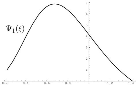
Figure 13: Behavior of the function $\Psi_{1}(\xi)=\psi_{1}(\xi)\,\exp\Bigl{(}3/8V(\xi)\Bigr{)}$ for the theory ${\lambda\over 4}\phi^{4}$ for $\lambda=0.3$; time $\tau$.

The solution is shown in Fig. 13. As before, we normalized $\Psi_{1}({\xi_{e}})=1$. One can easily see that, e.g., for $\lambda=0.3$, the function $\Psi_{1}({\xi})$ grows only $7$ times before it reaches its maximum. In the same interval, the function $\exp\Bigl{(}-3/8V(\xi)\Bigr{)}=\exp\Bigl{(}-{3\over 2\,\xi^{4}}\Bigr{)}$ grows $\sim 10^{1072}$ times. For $\lambda=10^{-4}$, the function $\Psi_{1}$ grows only $2300$ times, whereas the function $\exp\Bigl{(}-3/8V(\xi)\Bigr{)}$ grows $\sim 10^{3216996}$ times. This difference is much more dramatic than in the standard $t$-parametrization of time. It reflects the fact that in almost the whole interval from $\xi_{e}$ to $\xi\sim 0.65$, where the function $\psi_{1}({\xi})$ reaches its maximum, it is correctly described by the square of the tunneling wave function. In terms of the original variable $\chi$, this implies that in about one-third of the whole interval from $\chi_{e}=0.3$ to $\chi_{p}=({4/\lambda})^{1/4}$ the function $\psi_{1}({\chi})$ is given by the square of the tunneling wave function:

$$\psi_{1}(\chi)\sim\exp\Bigl{(}-{3\over 8V(\chi)}\Bigr{)}=\exp\Bigl{(}-{3\over 2\lambda\,\chi^{4}}\Bigr{)}~{}.$$ (146)

Thus, the square of the tunneling wave function does play an extremely important role in quantum cosmology. A more accurate fit to the function $\psi_{1}(\chi)$, which can be used in the whole interval from $\chi_{e}$ to $\chi_{p}$, is given by $\exp\Bigl{(}-{3\over 8V(\chi)}\Bigr{)}\,\Bigl{(}{1\over V(\chi)+0.4}-{1\over 1.4}\Bigr{)}$.

The resulting stationary distribution is

$$\tilde{P}_{p}(\phi,\tau\rightarrow\infty|\chi) \sim \exp\Bigl{(}-{3\over 8V(\chi)}\Bigr{)}\,\Bigl{(}{1\over V(\chi)+0.4}-{1\over 1.4}\Bigr{)}\,\cdot\,\phi\,\exp\Bigl{(}-{\pi\,(3-\lambda_{1})\phi^{2}}\Bigr{)}$$ (147)

$$= \exp\Bigl{(}-{3\over 2\lambda\,\chi^{4}}\Bigr{)}\,\Bigl{(}{4\over\lambda\chi^{4}+1.6}-{1\over 1.4}\Bigr{)}\,\cdot\,\phi\,\exp\Bigl{(}-3.5\sqrt{\lambda}\phi^{2}\Bigr{)}\ .$$

This expression is valid in the whole interval from $\phi_{e}$ to $\phi_{p}$ and it correctly describes asymptotic behavior of $\tilde{P}_{p}(\phi,\tau|\chi)$ both at $\chi\sim\chi_{e}$ and at $\chi\sim\chi_{p}$.

A similar investigation can be carried out for the theory $V(\phi)=V_{0}\ e^{\alpha\phi}$. The corresponding equations are

$$\psi_{1}^{\prime\prime}+\psi_{1}^{\prime}\left({\alpha\over 2}-{3\alpha\over 8V_{0}}e^{-\alpha\chi}\right)+\psi_{1}\ {3\pi(3-\lambda_{1})\over V_{0}}e^{-\alpha\chi}=0\ ,$$ (148)

$$\pi_{1}^{\prime\prime}+\pi_{1}^{\prime}\left({3\alpha\over 2}+{3\alpha\over 8V_{0}}e^{-\alpha\phi}\right)+\pi_{1}\left({\alpha^{2}\over 2}+{3\pi(3-\lambda_{1})\over V_{0}}e^{-\alpha\phi}\right)=0\ .$$ (149)

The (naive) boundary conditions are

$$\psi^{\prime}_{1}({\chi_{e}})={3\alpha e^{-\alpha\chi_{e}}\over 8V_{0}}\,\psi_{1}({\chi_{e}})\ ,~{}~{}~{}~{}~{}\psi_{1}(\chi_{p})=0\ ,$$ (150)

and

$$\pi^{\prime}_{1}({\phi_{e}})=-\,{\alpha\over 2}\,\pi_{1}({\phi_{e}})\ ,{}~{}~{}~{}~{}~{}\pi_{1}(\phi_{p})=0~{}.$$ (151)

The solution for $\psi_{1}(\chi)$ in the whole interval from $\chi_{e}$ to $\chi_{p}$ looks as follows:

$$\psi_{1}=\exp\Bigl{(}-{3\over 8V(\chi)}\Bigr{)}\,\Bigl{(}{1\over V(\chi)}-{1}\Bigr{)}=\exp\Bigl{(}-{3\,e^{-\alpha\chi}\over 8V_{0}}\Bigr{)}\,\Bigl{(}\frac{e^{-\alpha\chi}}{V_{0}}-1\Bigr{)}~{}.$$ (152)

The solution for $\pi_{1}(\phi)$ in the whole range from $\phi_{e}$ to $\phi_{p}$ with an accuracy of few percent is given by the following simple function:

$$\pi_{1}({\phi})=\Bigl{(}{1\over V(\phi)}-{1}\Bigr{)}\,V^{-1/2}(\phi)=V^{-3/2}_{0}\,\Bigl{(}e^{-\alpha\phi}-V_{0}\,\Bigr{)}\,e^{-\alpha\phi/2}\ .$$ (153)

Figure 14: Functions $\pi_{1}(\phi)$ and $\psi_{1}(\chi)$, representing the stationary solution $\tilde{P}_{p}(\phi,\tau|\chi)$ for the theory $V_{0}\,e^{\alpha\phi}$ with $V_{0}=0.1$, $\alpha=0.1$. The function $\tilde{\pi}_{1}(\phi)$ corresponds to the solution with improved boundary conditions.

The solutions are shown in Fig. 14. Note that now the solution for $\pi_{1}(\phi)$ is concentrated near the end of inflation, at $\phi\sim\phi_{e}$. The reason why we obtained such a solution is related to the ‘prescribed’ nature of the end of inflation in the theory with the exponential potential: Motion of the field is slow and diffusion is large until the very end of inflation at $\phi=\phi_{e}=0$. If the speed of motion of the field $\phi$ near the end of inflation had been vanishingly small, the distribution $\pi_{1}(\phi)$ would be equal to the square of the Hartle-Hawking wave function. For the exponential potential, however, this is not the case, see eq. (153).

As we mentioned at the end of the previous Section, when one describes inflation in the theory with the exponential potential, some care should be taken of boundary conditions. One should either modify the boundary conditions for the case of the exponential potential, or modify the effective potential itself. For example, one may study the theory with the effective potential $4V_{0}\,\sinh^{2}{\alpha\phi\over 2}$. However, this potential is considerably different from the exponential potential in a very large region $0<\phi\mathrel{\hbox{\hbox to0.0pt{\hbox{\lower 4.0pt\hbox{$\sim$}}\hss}\hbox{$<$}}}\alpha^{-1}$. This leads to a profound modification of the solutions, shifting the maximum of $\pi_{1}(\phi)$ towards $\phi>\alpha^{-1}\gg 1$. On the other hand, there is another way to modify the theory, by adding to it one more scalar field, which triggers a phase transition with an instantaneous end of inflation at $\phi=0$. Such a theory is described in Axions . In this case the potential of the field $\phi$ remains exponential at $\phi>0$. In order to obtain a phenomenological description of the end of inflation in this model one may assume that the derivative $V^{\prime}$ abruptly increases when the field $\phi$ becomes negative. In this case the boundary condition for the function $\pi_{1}$ becomes (compare with (131))

$$V^{1/2}(\phi)\ \left.\frac{\partial}{\partial\phi}\left({V^{1/2}(\phi)}\pi_{1}\right)\right|_{{\phi_{e_{+}}}}={3\over 8V(\phi)}\,\pi_{1}({\phi_{e_{-}}})\Bigl{(}V^{\prime}({\phi_{e_{-}}})-V^{\prime}({\phi_{e_{+}}})\Bigr{)}\ ,$$ (154)

where in our case $\phi_{e}=0$. The r.h.s. of this equation gives a positive contribution to the value of $\pi_{1}^{\prime}(\phi_{e})$ in eq. (151). The value of this contribution depends on the jump of $V^{\prime}$ at the point $\phi_{e}$. Numerical solution of the corresponding equation for different values of this jump shows that the solution remains unchanged in the main part of the interval from $\phi_{e}$ to $\phi_{p}$, except for a small vicinity of the point $\phi_{e}$, see Fig. 14. This again confirms that our solutions are rather robust with respect to the change of the boundary conditions at the end of inflation.

A complete stationary probability distribution is given by

$$\tilde{P}_{p}(\phi,\tau\rightarrow\infty|\chi) \sim \exp\Bigl{(}-{3\over 8V(\chi)}\Bigr{)}\,\Bigl{(}{1\over V(\chi)}-{1}\Bigr{)}\,\cdot\,\Bigl{(}{1\over V(\phi)}-{1}\Bigr{)}\,V^{-1/2}(\phi)$$ (155)

$$= V^{-5/2}_{0}\,\exp\Bigl{(}-{3\,e^{-\alpha\chi}\over 8V_{0}}\Bigr{)}\,\Bigl{(}e^{-\alpha\chi}-V_{0}\,\Bigr{)}\cdot\,\Bigl{(}e^{-\alpha\phi}-V_{0}\,\Bigr{)}\,e^{-\alpha\phi/2}\ .$$

This expression gives a rather good approximation for $\tilde{P}_{p}(\phi,\tau\rightarrow\infty|\chi)$ for all $\phi$ and $\chi$, except for a small vicinity of the point $\phi_{e}$ mentioned above.

Note, that the distributions which we obtained do depend on the choice of the time parametrization. This is not unexpected; each event may look differently being described in different coordinate systems. However, it would be very desirable to find an invariant description of our results. Fortunately, the most important qualitative results we discussed, the existence of the self-reproduction of the Universe and the existence of a stationary probability distribution $P_{p}$, do not depend on our choice of $t$- or $\tau$-parametrization of time.

VII Comments and Interpretation

The results obtained in this paper may seem strange and sometimes even counterintuitive. Therefore we are going to discuss their interpretation and an alternative derivation in a subsequent publication MezhLin . However, it is necessary to make some comments right now.

VII.1 Do we need Planck density to have stationarity?

There are two possible kinds of the stationarity. First of all, self-reproduction of inflationary domains implies that even in a very distant future there will be many inflationary domains in the Universe containing all possible values of scalar fields compatible with inflation. According to the no-hair theorem for de Sitter space, each such domain of a radius greater than $H^{-1}$ ($h$-region) will expand practically independently of the processes in the nearby domains. This means that the Universe will repeatedly reproduce inflationary domains, which will have statistically same properties as the similar domains produced billions of years ago.

This kind of stationarity is the most fundamental. Its existence is related only to the existence of the regime of self-reproduction. In all models we considered in this paper self-reproduction of inflationary domains occurs at $\phi>\phi^{*}$, where $V(\phi^{*})\ll 1$ b19 . Self-reproduction occurs also in the models where inflation is possible when the field $\phi$ is near a local maximum of its effective potential, at $V(\phi)\ll 1$ ArVil ; NewStationary ; such models originally were used in the new inflationary Universe scenario. Thus, the very existence of the process of self-reproduction of inflationary domains, and, consequently, the existence of the first, most fundamental stationarity, does not depend on unknown processes at $V(\phi)>1$. We will call this stationarity local, or microstationarity, to distinguish it from the global stationarity, or macrostationarity, which refers to stationarity of probability distributions over the whole Universe.

This second kind of stationarity may or may not exist. Its existence does not follow from any general considerations. This is similar to the situation in quantum statistics, where the description in terms of a macrocanonical ensemble sometimes is impossible despite the existence of a good description in terms of a microcanonical ensemble. On the other hand, in the situations where the Universe is globally stationary, the description of its evolution can be considerably simplified.

As we have seen, in all realistic inflationary models the probability distribution in comoving coordinates $P_{c}$ is not stationary. Fortunately, the probability distribution $P_{p}$ is stationary in many interesting cases.

First of all, it is stationary in the models where the inflaton field is fluctuating near a local maximum of its effective potential ArVil ; NewStationary . This is already extremely important. However, for the reason to be discussed in this Section, it would be most interesting to obtain stationary solutions in the theories where inflation is possible very close to $V(\phi)\sim 1$.

In this paper (see also MezhLinSmall ) we have found stationary solutions for $P_{p}$ in a class of models of chaotic inflation with the effective potentials ${\lambda\over 4}\phi^{4}$ and $V_{0}\,e^{\alpha\phi}$; a generalization for other theories will be considered in a separate publication MezhLin . The main assumption which we made to obtain these solutions is that the self-reproduction of inflationary domains is impossible (or at least is strongly hampered) at the density higher than the Planck density. We gave three different reasons why this assumption may be reasonable:

1. Diffusion equations for $P_{p}$ and our interpretation of their solutions it terms of the distribution of a classical field in a classical space do not work for $V(\phi)\mathrel{\hbox{\hbox to0.0pt{\hbox{\lower 4.0pt\hbox{$\sim$}}\hss}\hbox{$>$}}}1$. Therefore it seems that at the present level of our understanding of the Planckian physics the only thing one can do is to study only inflationary domains with $V(\phi)\mathrel{\hbox{\hbox to0.0pt{\hbox{\lower 4.0pt\hbox{$\sim$}}\hss}\hbox{$<$}}}1$ and discard those domains which jump to $V(\phi)\mathrel{\hbox{\hbox to0.0pt{\hbox{\lower 4.0pt\hbox{$\sim$}}\hss}\hbox{$>$}}}1$.

2. Large energy density concentrated in the spatial gradients of the scalar field fluctuations hampers the process of self-reproduction of inflationary domains with $V(\phi)\mathrel{\hbox{\hbox to0.0pt{\hbox{\lower 4.0pt\hbox{$\sim$}}\hss}\hbox{$>$}}}1$.

3. The only natural mass scale near the Planck density is the Planck mass. Therefore even if the effective potential is not very steep at small energy density, nothing can protect it from becoming very curved due to quantum gravity effects near the Planck density. In such a case inflation (or the process of self-reproduction of inflationary domains) will cease to exist at $V(\phi)\mathrel{\hbox{\hbox to0.0pt{\hbox{\lower 4.0pt\hbox{$\sim$}}\hss}\hbox{$>$}}}1$.

These arguments suggest that inflation (or at least self-reproduction of inflationary domains) cannot exist at $V(\phi)\mathrel{\hbox{\hbox to0.0pt{\hbox{\lower 4.0pt\hbox{$\sim$}}\hss}\hbox{$>$}}}1$. Therefore one should impose some boundary conditions which do not allow $P_{p}$ to penetrate deeply into the regions with $V(\phi)>1$. This immediately leads to the existence of stationary solutions for $P_{p}$ concentrated at $V(\phi)\mathrel{\hbox{\hbox to0.0pt{\hbox{\lower 4.0pt\hbox{$\sim$}}\hss}\hbox{$<$}}}1$. The exact form of these solutions does depend on the processes near the Planck boundary. However, as we will show in a separate publication MezhLin , in many cases this dependence is rather trivial and does not change the qualitative behavior of the stationary distribution $P_{p}$. For example, one can show that for each $\phi_{p}$ there exists such $\tilde{\phi}_{p}\sim\phi_{p}$ that imposing absorbing boundary conditions at $\phi_{p}$ gives the same solution for $\pi_{1}(\phi)$ as imposing reflecting boundary conditions at $\tilde{\phi}_{p}$. This means that the choice between absorbing and reflecting boundary conditions is equivalent to the corresponding redefinition of the position of the Planck boundary. Thus, even though a complete understanding of physical processes near the Planck boundary is important for obtaining exact stationary solutions for $P_{p}$, we do not expect that the qualitative features of these solutions in the region $\phi\ll\phi_{p}$ will be dramatically different from those which we obtained in the present paper.

One should keep in mind that in some theories the effective potential may become very steep at $\phi>\phi_{b}$ where $V(\phi_{b})\ll 1$, i.e. without any relation to quantum gravity effects and the Planck boundary. If this happens at $\phi_{b}>\phi^{*}$, then we will have a stationary distribution which is concentrated at $\phi\sim\phi_{b}$, and all our results will remain qualitatively correct after substituting $\phi_{b}$ instead of $\phi_{p}$. In particular, there will be a fractal geometry with a dimension $d_{fr}=\lambda_{1}$ (for $\tau$-parametrization of time), where $\lambda_{1}$ will be slightly less than $3$ (and, correspondingly, $d_{fr}=\frac{\lambda_{1}}{H(\phi_{b})}<3$ for $t$-parametrization).

On the other hand, there are some theories where the effective potential at large $\phi$ approaches some constant value $V_{0}\ll 1$. In such models nothing will prevent the distribution $P_{p}$ from moving towards indefinitely large $\phi$ without ever reaching the Planck boundary, and the global stationarity may be absent. Another class of models which may have runaway solutions are the models including interaction terms $\xi\phi^{2}R$. In such models the distribution $P_{p}$ is concentrated near the Planck boundary, but the Planck boundary is a line rather than a point, and there is a room for a runaway diffusion along this boundary LindeBellido .

VII.2 Is it possible to have stationarity and self-reproduction of the Universe at $\phi<\phi^{*}$?

In the first part of the paper we have shown that self-reproduction of the Universe occurs only if we have an inflationary domain with the field $\phi>\phi^{*}$. The critical field $\phi^{*}$ is typically much greater than $\phi_{e}$. For example, $\phi^{*}\sim 1/\sqrt{m}\gg\phi_{e}$ in the theory ${m^{2}\over 2}\phi^{2}$. However, we obtained a stationary probability distribution for all $\phi$ in the interval from $\phi_{e}$ to $\phi_{p}$. Does this mean that now we are taking our words back and saying that the self-reproduction of inflationary domains may occur at $\phi\ll\phi^{*}$ as well?

The answer to this question consists of two parts. First of all, for the existence of stationary distribution $\tilde{P}_{p}(\phi,t|\chi)$ at some field $\phi=\phi_{0}$ one does not need inflation and self-reproduction of the Universe at $\phi_{0}$. The distribution will remain stationary even for $\phi\ll\phi_{e}$, i.e. after the end of inflation. The stationarity of distribution at small $\phi$ is an automatic consequence of the stationarity of distribution at large $\phi$ and of the diffusion and rolling of the inflaton field from large $\phi$ towards small $\phi$. This is the reason why we obtained the same speed of growth of volume $e^{\lambda_{1}t}$ for all $\phi$. This implies also that the total volume of all parts of the Universe with $\rho\sim 10^{-29}$g$\cdot$cm^-3 should increase with the same speed. Indeed, according to our results, the total volume of the domains with $\phi=\phi_{e}$ at all times increases as $e^{\lambda_{1}t}$. But $10^{10}$ years later, the density of matter inside all such domains will become $\sim 10^{-29}$g$\cdot$cm^-3. It is obvious that since the total volume of the domains with $\phi=\phi_{e}$ permanently grows as $e^{\lambda_{1}t}$, the total volume of the all domains with $\rho\sim 10^{-29}$g$\cdot$cm^-3 will grow with exactly the same speed (with the time delay of $10^{10}$ years). Consequently, the relative fraction of volume of the parts of the Universe with any given properties (i.e. the total volume of the parts with the given properties, divided by $e^{\lambda_{1}t}$) is time-independent, even if these parts are post-inflationary.

Independently of this question, it is interesting to address the issue of self-reproduction of the parts of the Universe with $\phi<\phi^{*}$.

The critical field $\phi^{*}$ plays an important role when we study the possibility that the process of self-reproduction of inflationary domains begins from one domain of a size $O(H^{-1})$. Indeed, if we have one $h$-region with the field $\phi>\phi^{*}$, this is already enough to ensure the permanent self-reproduction of inflationary domains. However, soon after the beginning of this process there will be exponentially many domains with all values of the field $\phi$, including the field $\phi\sim\phi_{e}$. Typical quantum jumps of the field $\phi$ in such domains within the time $\Delta t\sim H^{-1}$ have the amplitude $\sim{H\over 2\pi}$, which is much smaller than the average classical decrease $\Delta\phi$ of the scalar field during this time

$$\Delta\phi=-{V^{\prime}\over 3H^{2}}=-{V^{\prime}\over 8\pi V}\ .$$ (156)

The end of inflation in a typical scenario is defined by the condition that the decrease of $V(\phi)$ within the Hubble time becomes comparable with $V(\phi)$:   $|\Delta V(\phi)|\sim V^{\prime}|\Delta\phi|\sim V(\phi)$. This gives $V^{\prime}\sim\sqrt{8\pi}V$, and $|\Delta\phi|\sim 1/\sqrt{8\pi}$ at the end of inflation. In all realistic models of inflation this decrease is much greater than the typical amplitude of fluctuations at the end of inflation, ${H\over 2\pi}\ll 1$.

However, if we already have many domains with $\phi\sim\phi_{e}$, then in some of these domains large jumps with an amplitude $\delta\phi\mathrel{\hbox{\hbox to0.0pt{\hbox{\lower 4.0pt\hbox{$\sim$}}\hss}\hbox{$>$}}}|\Delta\phi|\sim 1/\sqrt{8\pi}$ may occur. The probability of such jumps is exponentially suppressed, but once they occur and bring the field towards $\phi>\phi^{*}$, an infinite process of self-reproduction of inflationary domains begins again.

Let us first check whether such jumps are possible at all. There may exist quantum fluctuations with any amplitude. However, if the amplitude is too large, then the gradient energy density of these fluctuations becomes much greater than the potential energy density $V(\phi)$, and the standard approach we used in this paper should be considerably modified Creation . The boundary at which our ‘white noise’ becomes ‘not so white’ is determined by the condition ${1\over 2}(\partial_{i}\delta\phi)^{2}\sim{1\over 2}(H\delta\phi)^{2}\mathrel{\hbox{\hbox to0.0pt{\hbox{\lower 4.0pt\hbox{$\sim$}}\hss}\hbox{$<$}}}V(\phi)$, which gives $\delta\phi\mathrel{\hbox{\hbox to0.0pt{\hbox{\lower 4.0pt\hbox{$\sim$}}\hss}\hbox{$<$}}}\sqrt{6}/\sqrt{8\pi}$.

This means that the standard description of the fluctuations with $\delta\phi\sim\Delta\phi$ is valid for $\phi>\phi_{e}$, since $|\Delta\phi|<1/\sqrt{8\pi}$ at $\phi>\phi_{e}$. Therefore the portion of the original volume where the field $\phi$ within the typical time $\Delta t=H^{-1}$ experiences a jump up by $\delta\phi=C|\Delta\phi|\sim C/\sqrt{8\pi}$ is given by the Gaussian distribution

$$P(\phi\to\phi+\Delta\phi+\delta\phi)\sim\exp{\Bigl{(}-{(\delta\phi)^{2}\over 2<\phi^{2}>}\Bigr{)}}=\exp{\Bigl{(}-{2\pi^{2}(\delta\phi)^{2}\over H^{2}(\phi)}\Bigr{)}}=\exp{\Bigl{(}-{3C^{2}\over 32V(\phi)}\Bigr{)}}\ .$$ (157)

Here $C$ is some constant, which should be somewhat greater than $1$ if we wish that the field $\phi$ increases despite its decrease due to rolling down by $|\Delta\phi|\sim 1/\sqrt{8\pi}$:   $\delta\phi>|\Delta\phi|$. If we want the field $\phi$ to experience a subsequent jump by the same value $\delta\phi=C/\sqrt{8\pi}$, we should multiply our result by $\exp{\Bigl{(}-{3C^{2}\over 32V(\phi+\Delta\phi+\delta\phi)}\Bigr{)}}$. However, each of the subsequent jumps will be much more probable than the first one, since the degree of suppression is exponentially sensitive to the increase of $V(\phi+\Delta\phi+\delta\phi)$. Moreover, now the field should not jump so high to compete with the classical rolling, since the value of $\Delta\phi$ decreases at large $\phi$. Therefore, to a reasonable approximation, the probability of the first jump (157) gives us the whole result. (This estimate is particularly good for small initial $\phi\sim\phi_{e}$, which is comparable to $1/\sqrt{8\pi}$.) Thus, the portion of the original volume occupied by some field $\phi(t=0)\equiv\chi$, which experiences a series of jumps to $\phi^{*}$ (or to any other field $\phi>\chi$), is given by

$$P(\chi\to\phi)\sim\exp{\Bigl{(}-{3C^{2}\over 32V(\chi)}\Bigr{)}}\ .$$ (158)

With an accuracy of the factor $C=2$, this is just the square of the tunneling wave function!

This result implies that if we have an inflationary domain (or a collection of inflationary domains) of a total volume $\sim H^{-3}(\phi)\exp{\Bigl{(}+{3C^{2}\over 32V(\chi)}\Bigr{)}}$, some parts of this domain will enter eternal process of the self-reproduction of the Universe even if the field inside this domain initially was smaller than $\phi^{*}$.

VII.3 What about the Big Bang?

The main result of our work is that under certain conditions the properties of our Universe can be described by a time-independent probability distribution, which we have found for theories with polynomial and exponential effective potentials. A lot of work still has to be done to verify this conclusion. However, once this result is taken seriously, one should consider its interpretation and rather unusual implications.

When making cosmological observations, we study our part of the Universe and find that in this part inflation ended about $t_{e}\sim 10^{10}$ years ago. The standard assumption of the first models of inflation was that the total duration of the inflationary stage was $\Delta t\sim 10^{-35}$ seconds. Thus one could come to an obvious conclusion that our part of the Universe was created in the Big Bang, at the time $t_{e}+\Delta t\sim 10^{10}$ years ago. However, in our scenario the answer is somewhat different.

Let us consider an inflationary domain which gave rise to the self-reproduction of new inflationary domains. As we argued in Section 5.2, one can visualize self-reproduction of inflationary domains as a branching diffusion process. During this process, the first inflationary domain of initial radius $\sim H^{-1}(\phi)$ within the time $H^{-1}(\phi)$ splits into $e^{3}\sim 20$ independent inflationary domains of similar size. Each of them contains a slightly different field $\phi$, modified both by classical motion down to the minimum of $V(\phi)$ and by long-wavelength quantum fluctuations of amplitude $\sim H/2\pi$. After the next time step $H^{-1}(\phi)$, which will be slightly different for each of these domains, they split again, and so on. The whole process now looks like a branching tree growing from the first (root) domain. The radius of each branch is given by $H^{-1}$; the total volume of all domains at any given time $t$ corresponds to the ‘cross-section’ of all branches of the tree at that time, and is proportional to the number of branches. This volume rapidly grows, but when calculating it, one should take into account that those branches, in which the field becomes greater than $\phi_{p}$, die and fall down from the tree, and each branch in which the field becomes smaller than $\phi_{e}$, ends on an ‘apple’ (a part of the Universe where inflation ended and life became possible).

One of our results is that even after we discard at each given moment the dead branches and the branches with apples at their ends, the total volume of live (inflationary) domains will continue growing exponentially, as $e^{\lambda_{1}t}$. What is even more interesting, we have found that very soon the portion of branches with given properties (with given values of scalar fields, etc.) becomes time-independent. Thus, by observing any finite part of a tree at any given time $t$ one cannot tell how old the tree is.

To give the most dramatic representation of our conclusions, let us see where most of the apples grow. This can be done simply by integrating $e^{\lambda_{1}t}$ from $t=0$ to $t=T$ and taking the limit as $T\to\infty$. The result obviously diverges at large $T$ as $\lambda_{1}^{-1}\,e^{\lambda_{1}T}$, which means that most apples grow at an indefinitely large distance from the root. In other words, if we ask what is the total duration of inflation which produced a typical apple, the answer is that it is indefinitely long.

This conclusion may seem very strange. Indeed, if one takes a typical point in the root domain, one can show that inflation at this point ends within a finite time $\Delta t\sim 10^{-35}$ seconds. This is a correct (though model-dependent) result which can be confirmed by stochastic methods, using the distribution $P_{c}(\phi,\Delta t|\chi)$ b19 . How could it happen that the duration of inflation was any longer than $10^{-35}$ seconds?

The answer is related to the choice between $P_{c}$ and $P_{p}$, or between roots and fruits. Typical points in the root domain drop out from the process of inflation within $10^{-35}$ seconds. The number of those points which drop out from inflation at a much later stage is exponentially suppressed, but they produce the main part of the total volume of the Universe. Note that the length of each particular branch continued back in time may well be finite Vilenkin . However, there is no overall upper limit to the length of branches, and, as we have seen, the longest branches produce almost all parts of the Universe with properties similar to the properties of the part where we live now. Since by local observations we can tell nothing about our distance in time from the root domain, our probabilistic arguments suggest that the root domain is, perhaps, indefinitely far away from us. Moreover, nothing in our part of the Universe depends on the distance from the root domain, and, consequently, on the distance from the Big Bang.

Thus, inflation solves many problems of the Big Bang theory and ensures that this theory provides an excellent description of the local structure of the Universe. However, after making all kinds of improvements of this theory, we are now winding up with a model of a stationary Universe, in which the notion of the Big Bang loses its dominant position, being removed to the indefinite past.

But from inflation it also follows that on a much larger scale the Universe is extremely inhomogeneous. In some parts of the Universe the energy density $\rho$ is now of the order of one (in Planck units), which is 123 orders of magnitude higher than the $\sim 10^{-29}g\cdot cm^{-3}$ we can see nearby. In such a scenario there is no reason to assume that the Universe was initially homogeneous and that all of its causally disconnected parts started their expansions simultaneously.

There is one subtle point in this discussion. According to our picture, the main part of the volume of the Universe is being produced by inflation not very far from the Planck boundary. Indeed, imagine that we imposed our absorbing or reflecting boundary conditions not at $V(\phi_{p})=1$, but at $V(\bar{\phi}_{p})=1/4$, thus excluding from our consideration those branches where the energy density may become greater than $V(\bar{\phi}_{p})=1/4$. This would reduce the eigenvalue $\lambda_{1}$ approximately by a factor of $2$: $\bar{\lambda}_{1}\sim{1\over 2}\lambda_{1}$. Correspondingly, the total volume of the Universe would grow not as $e^{\lambda_{1}t}$, but at a much slower rate $e^{\bar{\lambda}_{1}t}$. This means that the main contribution to the total volume of the Universe is given by the branches which from time to time come very close to the state of the maximal possible energy density compatible with the self-reproduction of inflationary domains. In Section 4 we called such states ‘Small Bangs’; they correspond to the peaks of the mountains on Figs. 3.6 and 7.5.

Therefore even though the original Big Bang singularity may be removed to the indefinite past, the typical time lapse from the last Small Bang to the end of inflation may be as small as $10^{-35}$ seconds. From the point of view of a present observer, there is no much difference between the last Small Bang and the original Big Bang; thus one may still use the old Big Bang theory for a phenomenological description of the observational data. However, if one wishes to understand the global structure of the Universe, its beginning and its fate, one should use a more complete theory including quantum cosmology.

The difference between the Big Bang and the Small Bangs is especially clear in the theories where there exists a large difference between the maximal possible value of $V(\phi)$ compatible with inflation and the Planck density. This is the case in the theories with the potentials which have a local maximum at some $\phi$, or which approach a plateau with $V(\phi)=V_{0}\ll 1$ at large $\phi$, or which become very steep at $\phi>\phi_{b}$, where $\phi^{*}\ll\phi_{b}\ll\phi_{p}$. In such theories inflationary quantum fluctuations never bring the Universe back to the Planck density. However, as we have argued, this difference may exist even in such theories as $\phi^{n}$ and $e^{\alpha\phi}$. The Big Bang is believed to be the single event of creation of the very first domains of classical space-time; the description of these domains in terms of classical space-time was impossible before the Big Bang. Meanwhile, each branch may come through the state which we call ‘Small Bang’ many times; the more times each branch approaches the state of maximal density compatible with inflation, the greater contribution to the total volume of the Universe it gives.

VII.4 Initial conditions for inflation, different versions of inflationary theory and observational data

Even though the properties of the Universe around us do not depend on the time from the Big Bang to the present epoch, one may still try to examine the problem of initial conditions near the cosmological singularity. However, as we argued above, a more relevant problem would be to find typical trajectories (branches) which could produce a part of the Universe of our type. Some aspects of this problem can be studied with the help of the probability distribution ${P}_{p}(\phi,t|\chi)$, or with the help of the function $\psi_{1}(\chi)$.

Let us consider for example the classical potential of the Coleman-Weinberg type used in the new inflationary theory

$$V(\phi)=\lambda\left(\phi^{4}\ln{\phi\over\sigma}-{\phi^{4}\over 4}+{\sigma^{4}\over 4}\right)~{}.$$ (159)

Here $\phi\geq 0$;  the field $\sigma\ll 1$ corresponds to the minimum of the effective potential (159). In the new inflationary Universe scenario it was assumed that the high temperature effects put the field $\phi$ onto the top of the effective potential at $\phi=0$, and then inflation begins as the temperature drops down b16 . However, it was soon realized that this scenario usually does not work, and one should consider chaotic inflation instead. According to this scenario, one can have two different possibilities to obtain inflation in the theory (159): One may consider inflationary domains where the Universe from the very beginning was in a state close to $\phi=0$, or domains with $\phi\mathrel{\hbox{\hbox to0.0pt{\hbox{\lower 4.0pt\hbox{$\sim$}}\hss}\hbox{$>$}}}1$ b17 ; Chaot2 . Whereas both possibilities in principle can be realized, the second one appears to be much more probable from the point of view of initial conditions. As we argued in Section 2, initial conditions which are necessary for inflation naturally appear if inflation may begin at $V(\phi)\sim 1$, i.e. close to the Planck density. On the other hand, the probability of inflation seems to be exponentially suppressed if it may begin only at $V(\phi)\ll 1$, which typically is the case if it begins at $\phi=0$. This conclusion follows from many different arguments, including the qualitative discussion of possible initial conditions near the singularity b17 ; ExpChaot , calculation of the tunneling wave function of the Universe b56 –b59 , and even from the computer simulation of different regimes of the Universe expansion Piran . Did we learn anything new about it after the present work?

First of all, our results give some additional indication of importance of the tunneling wave function, since its square appears in the expression for $\psi_{1}(\chi)$. This may be considered as a new confirmation of our conjecture that the most natural realization of chaotic inflation scenario in the theory (159) occurs if inflation begins near the Planck density, at $\lambda\phi^{4}\ln{\phi\over\sigma}\sim 1$, i.e. at $\phi\gg 1$.

However, now we can say even more. If we examine the solutions of the diffusion equation for $P_{p}$ in this model we would find that these solutions consist of two independent branches. The field $\phi$ in the domains with $\phi<\sigma$ never diffuses to $\phi>\sigma$, and vice versa. Correspondingly, the distribution $P_{p}(\phi,t|\chi)$, which gives the total volume occupied by the field $\phi$, will consist of two branches:

$$P^{+}_{p}(\phi,t|\chi)=e^{\lambda_{1}^{+}t}\pi_{1}^{+}(\phi)\psi_{1}^{+}(\chi)~{}~{}~{}~{}\mbox{for}~{}~{}~{}~{}\phi,\chi>\sigma{}~{},$$ (160)

and

$$P^{-}_{p}(\phi,t|\chi)=e^{\lambda_{1}^{-}t}\pi_{1}^{-}(\phi)\psi_{1}^{-}(\chi)~{}~{}~{}~{}\mbox{for}~{}~{}~{}~{}\phi,\chi<\sigma~{}.$$ (161)

The eigenvalue $\lambda_{1}^{-}$ is approximately equal to $3H(\phi=0)\ll 1$ ArVil ; NewStationary , whereas from our results it follows that $\lambda_{1}^{+}\sim 1$. This means that if the Universe originally contained both domains with $\phi>\sigma$ and with $\phi<\sigma$, then within a very short time of the order of the Planck time $t\sim 1$, the main part of the volume of the Universe becomes totally dominated by domains with $\phi>\sigma$.

Using the analogy between the Universe and the growing tree, let us imagine that the branches with $\phi>\sigma$ are green, and the branches with $\phi<\sigma$ are red. Our results imply that if the Universe originally contained at least one green branch, then very soon it becomes all green, independently of the original number of red branches (which in fact should be smaller than the original number of green branches if our previous arguments concerning initial conditions are correct).

This conclusion may be somewhat modified if one takes into account a possibility of large jumps of the field $\phi$ over the non-inflationary region near $\sigma$. Note that the width of this region is very large, $\Delta\phi\sim 1$, and since this region is not inflationary, our methods do not allow any description of such jumps. If such jumps are possible, for example, due to the process described in Creation , or due to Euclidean tunneling, then green branches will produce red off-springs, and the total volume of the red domains will grow with the same speed as the total volume of the green domains. However, even if this process is possible, the total volume of domains $\phi<\sigma$ will remain exponentially small as compared with the volume of domains with $\phi>\sigma$ because of the exponentially small probability of such large jumps Creation .

Suppose now that the effective potential $V(\phi)$ (159) at large $\phi$ grows not as $\lambda\phi^{4}\ln{\phi\over\sigma}$ but, for example, as $e^{\alpha\phi}$ with $\alpha\mathrel{\hbox{\hbox to0.0pt{\hbox{\lower 4.0pt\hbox{$\sim$}}\hss}\hbox{$>$}}}\sqrt{16\pi}$, or in any other way which precludes inflation (or self-reproduction of inflationary domains) at $\phi>\sigma$. Then, in the absence of any competition, the red branches (beginning at $\phi\ll\sigma$) will win. Of course, this will happen only if initial conditions are good enough for inflation to begin at $\phi=0$. As we just argued, this probability is exponentially small. However, we are speaking about the conditional probability that our part of the Universe was formed by inflationary expansion, as compared with the probability that it was formed by some non-inflationary process. This suggests that in order to compare these probabilities one should multiply the probability of having given initial conditions by the subsequent increase of the volume of any part of the Universe with these initial conditions, and then normalize the total probability by dividing it by the total volume of the Universe. This was our method of obtaining the normalized probability distribution $\tilde{P}_{p}$. If this is correct, then the self-reproducing inflationary branches always win. Indeed, whatever is the probability of proper initial conditions for inflation beginning at $V(\phi)\ll 1$, the main contribution to the total volume of the Universe will be given by self-reproducing inflationary domains, since this contribution even now continues growing exponentially as $e^{\lambda_{1}t}$, and only this contribution will survive after the division by $e^{\lambda_{1}t}$.

Thus, it may be possible to have a consistent cosmological theory even if inflation occurs only at $V(\phi)\ll 1$. This is the case, e.g., for the ‘natural inflation’ Natural and for the hyperextended inflation Hext . However, as we have seen, realization of inflation in these models requires somewhat trickier reasoning than in the theories where inflation is possible at $V(\phi)\sim 1$. What if the Universe was created in a non-inflationary state, because of the exponential suppression $\sim e^{-3/8V(\phi)}$ of the probability to produce an inflationary Universe with small $V(\phi)$? Does it make sense to multiply the volume of an unborn inflationary Universe by $e^{\lambda_{1}t}$? Even though we believe that this is a wrong objection and that the indefinitely large growth of volume produced by inflation does solve the problem of initial conditions for every theory where the self-reproduction of the Universe is possible Mijic ; MyBook , it would be desirable to have an alternative realization of chaotic inflation scenario, where initial conditions for inflation would appear in a natural way even if inflation driven by the field $\phi$ may occur only at $V(\phi)\ll 1$.

Fortunately, this task can be easily fulfilled Axions ; TwoFields . The simplest way to do it is to introduce an additional scalar field $\Phi$, which may have no interaction with the field $\phi$, but which can drive inflation at $V(\Phi)\sim 1$. In such a theory inflation may begin at $V(\Phi)\sim 1$ in a quite natural way. This may be a ‘bad’ inflation, producing large perturbations ${\delta\rho\over\rho}\gg 10^{-5}$. However, in the process of indefinitely long inflation driven by the field $\Phi$, fluctuations of the scalar field $\phi$ are produced, which in some domains of the Universe put the field $\phi$ on the top of its effective potential. In those domains where the heavy field $\Phi$ rolls down to the minimum of $V(\Phi)$, inflation continues due to the light field $\phi$, which determines the properties of the observable part of our Universe. Models of this type were called ‘hybrid inflation’ in ref. Axions .

Let us consider, for example, the ‘natural inflation’ model, which has an inflaton potential of the type

$$V(\Phi)=V_{0}~{}\left(1-\cos{\Phi\over\Phi_{0}}\right)~{}.$$ (162)

This is exactly the model which we considered in our computer simulation of production of the axionic domain walls during inflation driven by the field $\phi$, see Section 3.4. Black lines in Fig. 5 correspond to the parts of the Universe where $\Phi=\pi(2n+1)$, i.e. where quantum fluctuations have driven the field $\Phi$ onto the top of its effective potential. In the comoving coordinates these black lines look very thin, but one should remember that they are always much thicker than $H^{-1}$. In those parts of the Universe where the field $\phi$ eventually rolls down to the minimum of its effective potential, inflation still continues in the black regions with $\Phi=\pi(2n+1)$. The Universe in these regions enters the process of eternal self-reproduction. After a while, the parts of the Universe produced by these black regions enter a stationary regime, in which nothing depends on the first stages of inflation driven by the field $\phi$. This exactly corresponds to the scenario we discussed in the previous paragraph, up to an obvious redefinition $\phi\leftrightarrow\Phi$.

Of course, there will be many other parts of the Universe where at the end of inflationary stage driven by the field $\phi$, the field $\Phi$ will not stay on the top of the effective potential (162). The volume of such parts at the end of the first stage of inflation will be greater than the volume of the parts with $|\Phi-\pi(2n+1)|\mathrel{\hbox{\hbox to0.0pt{\hbox{\lower 4.0pt\hbox{$\sim$}}\hss}\hbox{$<$}}}H$ by a factor $\sim\Phi_{0}/H\gg 1$. This is reflected by the relatively large area painted white in Fig. 5. However, the regions with $|\Phi-\pi(2n+1)|\mathrel{\hbox{\hbox to0.0pt{\hbox{\lower 4.0pt\hbox{$\sim$}}\hss}\hbox{$<$}}}H$ (painted black in Fig. 5) enter the process of self-reproduction, and very soon the main part of the volume of the Universe (at a given value of the field $\phi$) will be dominated by domains produced by inflation of these black regions.

Thus, even though the ‘natural inflation’ model does not look natural at all from the point of view of initial conditions, it can be incorporated into a chaotic inflation scenario of a more general type where the problem of initial conditions can be easily solved. According to this scenario, we live in the remnants of the domain walls produced at the first stage of inflation.

Our main conclusion is that whenever one may have two different inflationary branches, the main contribution to the total volume of the Universe will be given by the branch on which inflation may occur at a greater value of $V(\phi)$. The initial conditions for inflation on this branch are also more natural. However, it is possible to construct consistent inflationary models in which our part of the Universe is produced by a branch where inflation may occur only at very small $V(\phi)$.

The main motivation for our investigation was a desire to get a complete and internally consistent picture of the global structure of the Universe. However, sometimes the knowledge of the global structure of the Universe may tell us something nontrivial about its local structure. For example, let us consider the ratio of adiabatic perturbations to gravitational waves, or the ratio between scalar and tensor perturbations of metric. Is it possible to find a model-independent relation between these perturbations Davis ; Kolb ?

In some models this relation may depend not only on the choice of the potential, but also on the initial conditions for inflation. In particular, the amplitude and spectrum of adiabatic perturbations produced at the last stages of inflation in the theory (159) do not depend strongly on whether inflation begins at $\phi\ll\sigma$ or at $\phi\gg\sigma$. In both cases ${\delta\rho\over\rho}\sim\sqrt{\lambda}~{}\log^{3/2}l$  MyBook . However, the amplitude of gravitational waves produced during the rolling from $\phi>\sigma$ will be proportional to $H(\phi\sim M_{p})=O(\sqrt{\lambda})$, whereas the amplitude of gravitational waves produced during the rolling from $\phi<\sigma$ is proportional to $H(\phi=0)\sim\sqrt{\lambda}\phi^{2}_{0}\ll\sqrt{\lambda}$. Without saying anything about initial conditions and about the process of self-reproduction of the Universe in this theory, one cannot have a definite prediction of the amplitude of gravitational waves and of the ratio of tensor perturbations of metric to the scalar ones in this model. However, as we have argued, the main part of the volume of the Universe is produced by inflation along the branches with $\phi>\sigma$. This enables us to make a definite prediction of the amplitude of tensor perturbations in this model: this amplitude should be proportional to $\sqrt{\lambda}$ rather than to $\sqrt{\lambda}\phi^{2}_{0}$.

This example shows that the investigation of the global structure of inflationary Universe, which at the first glance deals with the scales which we will never observe, may lead to testable predictions. In what follows we will discuss a much more speculative possibility, which, however, may deserve future investigation.

Until now, most of the studies of properties of the observable part of the Universe were to some extent related to the distribution $P_{c}$. It was assumed that one should take a typical sample of inflationary Universe, study its evolution and predict its properties. However, our investigation shows that the field distributions which seem typical from the point of view of $P_{c}$, may happen to be very unusual from the point of view of $P_{p}$, and vice versa. What if we live in a part of the Universe which is very unusual from the ‘normal’ point of view, reflected in the distribution $P_{c}$?

We have discussed already the most dramatic difference between $P_{c}$ and $P_{p}$. A trajectory which is typical from the point of view of $P_{c}$ corresponds to the duration of inflation $\sim 10^{-35}$ seconds, whereas from the point of view of $P_{p}$ a typical trajectory spends an indefinitely long time in the inflationary regime near the Planck boundary. Analogously, the standard investigation of density perturbations suggests that the typical deviation of the density of the Universe from the critical density cannot exceed ${\delta\rho\over\rho}\sim 10^{-5}$ on the scale of the horizon. The question we would like to address is whether there may exist some reason for us to live in a not very typical domain, where the deviation of density from the critical density might be greater than $10^{-5}$. The reason why this might happen can be explained as follows. If one tries to find out those trajectories which give the dominant contribution to the total volume of the Universe within a given time interval $t$, one may conclude that if the time $t$ is sufficiently large, then the main contribution will be given by the trajectories which first rush up towards the highest possible values of $V(\phi)$, spend there as long time as possible, and at the very last moment rush down towards small $\phi$ with the speed even somewhat greater than the speed of the classical rolling. Indeed, even though the probability of such a regime is exponentially suppressed, those lucky trajectories, which happen to follow these rules of the game and saved some time in the process of rolling down, may become generously rewarded by the additional exponentially large growth of volume during the extra time they spend near the highest possible values of $V(\phi)$.

If this is the case, the main contribution to the volume of the Universe at a given time $t$ in a state with a given density $\rho$ will be given by the rare regions where the field $\phi$ at the last stages of inflation jumped down with the speed exceeding its speed of the nearby domains. Thus, the energy density inside these regions should be somewhat smaller than the energy density in their neighborhood. However, not every jump down may compensate the delay in the homogeneous classical rolling. The proper jump should result in a nearly homogeneous decrease of density on a scale comparable to the scale of the horizon. A region where such a jump took place will look now like a part of an open Universe. Such regions will be spherically symmetric, since the probability of formation of asymmetric regions by quantum jumps will be suppressed by a large exponential factor, just as the probability of formation of asymmetric bubbles during the first order phase transitions.

Needless to say, this scenario is extremely speculative. Moreover, a preliminary investigation of this effect indicates that in the simple theories with $V(\phi)\sim\phi^{n}$ the corresponding effect is insignificant. The only theories where this effect might be considerable are those where the Hubble constant at the last stages of inflation is very small. However, the possibility that we may live in a locally open part of inflationary Universe, i.e. in a part with $\Omega<1$, should not be overlooked. In order to study it in a proper way, one needs to know not only the probability distribution $P_{p}$, but also the correlation functions for the values of the field $\phi$ at different points, taking into account different rate of expansion of the Universe along different inflationary trajectories. We hope to return to a discussion of this possibility in a separate publication.

VIII Brief Summary

The history of the development of cosmology seems to follow a very nontrivial path. At the beginning of the century many people tried to find a stationary solution of the Einstein equations, with the hope that General Relativity would resolve the inability of Newton’s theory to provide us with a stationary cosmological model. Einstein even introduced the cosmological constant into his theory for this purpose. The non-stationary character of the Big Bang theory advocated by Gamov on the basis of Friedmann cosmological models seemed very unpleasant to many scientists in the fifties. Then, the discovery of the cosmic microwave background turned the situation upside down. Physicists began to treat with contempt any attempts to find stationarity (remember the ‘steady-state’ model). After several decades of the reign of the Big Bang theory, the inflationary scenario appeared, which solved many of the intrinsic problems of the Big Bang cosmology and apparently removed the last doubts concerning its validity.

However, it was realized soon afterwards, that inflation is even more dynamic than the old Big Bang theory. In inflationary cosmology, in addition to the ordinary classical evolution of the Universe governed by the Einstein equation, quantum mechanical evolution proves to be extremely important, being responsible for the large-scale structure formation and even for the global structure of the Universe. This quantum mechanical evolution can be approximately described by stochastic methods, and some of the solutions of the corresponding stochastic equations prove to be stationary! Surprisingly enough, after the dramatic development of the Big Bang theory during the last ten years, we are coming now to a new formulation of the stationary cosmology, on a new level of understanding and without losing a single achievement of our predecessors. The observable part of the Universe can be very well described by the homogeneous isotropic Big Bang model. However, on extremely large scales (far beyond the visible horizon) the Universe is very inhomogeneous. On even larger scales this inhomogeneity produces a kind of fractal structure, repeating itself on larger and larger time and length scales. The statistical properties of this structure are what we have found to be stationary.

Of course, we are far from giving final answers to fundamental questions of cosmology. In fact, we are just beginning to learn how to ask proper questions in the context of the new cosmological paradigm. We need to make sure that our results have correct quantum mechanical interpretation. It would be important to find an invariant way of formulating our results, which would not depend on a particular choice of time parametrization. There are many other problems related to our approach which are to be solved. We know, however, that at the first stage of any investigation in quantum field theory or in quantum statistics it makes a lot of sense to find a vacuum state, or a state of thermal equilibrium, or any stationary state which may play the role of a ground state of the system. We hope very much that the existence of the stationary regime of the evolution of the Universe described in this paper may help us to find a proper framework for the future investigation of quantum cosmology.

It is a pleasure to thank J. Bond, S. Hawking, M. Mijić, D. Page, A. Starobinsky and A. Vilenkin for valuable discussions. This work was supported in part by NSF grant PHY-8612280.

References

-
(1)
E.B. Gliner, Sov. Phys. JETP 22, 378 (1965); Dokl.
Akad.
Nauk USSR 192, 771 (1970);
E.B. Gliner and I.G. Dymnikova, Pis. Astron. Zh. 1, 7 (1975);
I.E. Gurevich, Astrophys. Space Sci. 38, 67 (1975). - (2) A.A. Starobinsky, JETP Lett. 30, 682 (1979); Phys. Lett. 91B, 99 (1980).
- (3) A.H. Guth, Phys. Rev. D23, 347 (1981).
-
(4)
A.D. Linde, Phys. Lett. 108B, 389 (1982); 114B, 431
(1982); 116B, 335, 340 (1982);
A. Albrecht and P.J. Steinhardt, Phys. Rev. Lett. 48, 1220 (1982). - (5) A.D. Linde, Phys. Lett. 129B, 177 (1983).
- (6) D. La and P.J. Steinhardt, Phys. Rev. Lett. 62, 376 (1989).
-
(7)
A.D. Linde, Particle Physics and Inflationary
Cosmology (Harwood, Chur, Switzerland, 1990);
A.D. Linde, Inflation and Quantum Cosmology (Academic Press, Boston, 1990). - (8) P.J.E. Peebles, Principles of Physical Cosmology, (Princeton University Press, Princeton, 1993).
- (9) A.D. Linde, Phys. Lett. 175B, 395 (1986); Physica Scripta T15, 169 (1987); Physics Today 40, 61 (1987).
- (10) A.S. Goncharov and A.D. Linde, Sov. Phys. JETP 65, 635 (1987); A.S. Goncharov, A.D. Linde and V.F. Mukhanov, Int. J. Mod. Phys. A2, 561 (1987).
- (11) Ya. B. Zeldovich, Sov. Astron. Lett. 7, 322 (1981); L.P. Grishchuk and Ya. B. Zeldovich, in: Quantum Structure of Space-Time, edited by M. Duff and C. J. Isham, Cambridge University Press, Cambridge (1983), p. 353.
- (12) A. Vilenkin, Phys. Lett. B117, 25 (1982).
- (13) A.D. Linde, JETP 60, 211 (1984); Lett. Nuovo Cim. 39, 401 (1984).
- (14) Ya.B. Zeldovich and A.A. Starobinsky, Sov. Astron. Lett. 10, 135 (1984).
- (15) V.A. Rubakov, Phys. Lett. 148B, 280 (1984).
- (16) A. Vilenkin, Phys. Rev. D30, 549 (1984).
- (17) P.J. Steinhardt and M.S. Turner, Phys. Rev. D29, 2164 (1984).
- (18) P. Collins and R. Langbein, Phys. Rev. D45, 3429 (1992); ibid D47, 2302 (1993).
- (19) A.D. Linde, Phys. Lett. 132B, 317 (1983).
- (20) A.D. Linde, Phys. Lett. 162B, 281 (1985).
- (21) J. Halliwell, Phys. Lett. B185, 341 (1987); A.B. Burd and J.D. Barrow, Nucl. Phys. B308, 929 (1988); A.R. Liddle, Phys.Lett. B220, 502 (1989).
- (22) L. Abbott and M. Wise, Nucl. Phys. B244, 541 (1984); F. Luccin and S. Matarrese, Phys. Rev. D32, 1316 (1985).
- (23) J.D. Barrow and A. Ottewill, J. Phys. A16, 2757 (1983); A.A. Starobinsky, Sov. Astron. Lett. 9, 302 (1983); L.A. Kofman, A.D. Linde, and A.A. Starobinsky, Phys. Lett. 157B, 36 (1985).
- (24) A.D. Linde, Phys. Lett. 132B, 317 (1983); R. Holman, P. Ramond and G.G. Ross, Phys. Lett. B137, 343 (1984); A.S. Goncharov and A.D. Linde, Phys.Lett. 139B, 27 (1984); Class. Quantum Grav. 1, L75 (1984).
- (25) K. Freese, J.A. Frieman and A.V. Olinto Phys. Rev. Lett. 65, 3233 (1990); F.C. Adams., J.R. Bond, K. Freese, J.A. Frieman and A.V. Olinto Phys. Rev. D47, 426 (1993).
- (26) A.D. Linde, Phys. Lett. B238, 160 (1990); ibid B249, 18 (1990).
- (27) A.D. Linde, Phys.Lett. B259, 38 (1991).
-
(28)
A.H. Guth, Phys. Rev. D23, 347 (1981);
J.R. Gott, Nature 295, 304 (1982);
K. Sato, H. Kodama, M. Sasaki and K. Maeda, Phys. Lett. B108, 35 (1982). -
(29)
P.J. Steinhardt, in The Very Early Universe, G.W.
Gibbons, S.W. Hawking, S. Siklos, eds., Cambridge U.P. Cambridge,
England (1982), p. 251;
A.D. Linde, Nonsingular Regenerating Inflationary Universe, Cambridge University preprint (1982). - (30) A. Vilenkin, Phys. Rev. D27, 2848 (1983).
-
(31)
J.A. Wheeler, in: Relativity, Groups and
Topology
eds. C.M. DeWitt and J.A. Wheeler (Benjamin, New York, 1968);
B.S. DeWitt, Phys. Rev. 160, 1113 (1967). - (32) D.N. Page, Phys. Rev. D32, 2496 (1985).
- (33) J.B. Hartle and S.W. Hawking, Phys. Rev. D28, 2960 (1983).
- (34) A.A. Starobinsky, in: Fundamental Interactions (MGPI Press, Moscow, 1984), p. 55.
- (35) A.S. Goncharov and A.D. Linde, Sov. J. Part. Nucl. 17, 369 (1986).
- (36) A.A. Starobinsky, in: Current Topics in Field Theory, Quantum Gravity and Strings, Lecture Notes in Physics, eds. H.J. de Vega and N. Sanchez (Springer, Heidelberg 1986) 206, p. 107.
- (37) M. Aryal and A. Vilenkin, Phys. Lett. B199, 351 (1987).
-
(38)
Y. Nambu and M. Sasaki, Phys.Lett. B219, 240
(1989);
Y. Nambu, Prog. Theor. Phys. 81, 1037 (1989). - (39) M. Sasaki, Y. Nambu and K. Nakao, Phys. Lett. B209, 197 (1988); Nucl. Phys. B308, 868 (1988).
- (40) K. Nakao, Y. Nambu and M. Sasaki, Prog. Theor. Phys. 80, 1041 (1988).
- (41) M. Mijić, Phys. Rev. D42, 2469 (1990); Int. J. Mod. Phys. A6, 2685 (1991).
- (42) A.D. Linde and A. Mezhlumian, Phys. Lett. B307, 25 (1993).
- (43) A.D. Linde and A. Mezhlumian, in preparation.
- (44) A.D. Linde and D.A. Linde, in preparation.
- (45) E.W. Kolb and M.S. Turner, The Early Universe (Addison-Wesley, New York, 1990).
- (46) J.H. Kung and R.H. Brandenberger, Phys.Rev. D42, 1008 (1990); ibid D40, 2532 (1989); D.S. Goldwirth and T. Piran, Phys. Rept. 214, 223 (1992).
- (47) T.S. Bunch and P.C.W. Davies, Proc. Roy. Soc. A360, 117 (1978); A. Vilenkin and L. Ford, Phys. Rev. D26, 1231 (1982); A.D. Linde, Phys. Lett. 116B, 335 (1982); A.A. Starobinsky, Phys. Lett. 117B, 175 (1982); A. Vilenkin, Nucl. Phys. B226, 527 (1983).
- (48) V.F. Mukhanov and G.V. Chibisov, JETP Lett. 33, 523 (1981); S.W. Hawking, Phys. Lett. 115B, 339 (1982); A.A. Starobinsky, Phys. Lett. 117B, 175 (1982); A.H. Guth and S.-Y. Pi, Phys. Lett. 49, 1110 (1982); J. Bardeen, P.J. Steinhardt and M. Turner, Phys. Rev. D28, 679 (1983); V.F. Mukhanov, JETP Lett. 41, 493 (1985).
- (49) A.D. Linde, Nucl. Phys. B372, 421 (1992).
- (50) J.J. Halliwell and J.B. Hartle, Phys. Rev. D41, 1815 (1990).
- (51) P.J. Steinhardt and F.S. Acetta, Phys. Rev. Lett. 64, 2740 (1990).
- (52) B. Spokoiny, Kyoto University preprint No 1192 (1993), hep-th/9305158.
- (53) Ya.B. Zeldovich and A.D. Linde, unpublished (1986).
- (54) D.S. Salopek and J.R. Bond, Phys. Rev. D42, 3936 (1990); ibid D43, 1005 (1991).
- (55) G. David, Wavelets and Singular Integrals on Curves and Surfaces, (Springer-Verlag, Berlin, 1991).
- (56) L.A. Kofman and A.A. Starobinsky, Phys. Lett. B188, 399 ( 1987).
- (57) P. Sikivie, Phys. Rev. Lett. 48, 1156 (1982).
- (58) A.D. Linde and D. Lyth, Phys. Lett. B246, 353 (1990).
- (59) A. Mezhlumian and S.A. Molchanov, J. Stat. Phys. 71, 799 (1993).
-
(60)
B.A. Sevastyanov, Branching Processes
(Moscow, Nauka,1971);
N. Ikeda and S. Watanabe, Stochastic Differential Equations and Diffusion Processes (North-Holland, Amsterdam, 1981). - (61) C.W. Gardiner, Handbook of Stochastic Methods, (Springer-Verlag, Berlin, 1985).
- (62) M. A. Markov, Ann. Phys. 155, 333 (1984).
- (63) V. Mukhanov and R. Brandenberger, Phys. Rev. Lett. 68, 1969 (1992); R. Brandenberger, V. Mukhanov and A. Sornborger, Brown University Preprint BROWN-HET-891, gr-qc/9303001, (1993).
- (64) D.J. Gross and P.F. Mende, Nucl.Phys.B303, 407 (1988). D. Amati, M. Ciafaloni and G. Veneziano, Phys.Lett. 197B, 81 (1987); Phys.Lett. B289, 87 (1992); M. Gasperini and G. Veneziano, Phys.Lett. B277, 256 (1992).
- (65) R. Brandenberger and C. Vafa, Nucl. Phys., B316, 391 (1989).
- (66) J. Garcia-Bellido and A.D. Linde, in preparation.
- (67) A. Vilenkin, Phys. Rev. D46, 2355 (1992).
- (68) A.D. Linde, Phys.Lett. B202, 194 (1988).
- (69) R.L. Davis, H.M. Hodges, G.F. Smoot, P.J. Steinhardt and M.S. Turner, Phys. Rev. Lett. 69, 1856 (1992).
- (70) E.J. Copeland., E.W. Kolb, A.R. Liddle and J.E. Lidsey, Sussex University preprint SUSSEX-AST-93-3-1 (1993), hep-ph/9303288.
- (71) M. Sasaki, Kyoto University preprint, in preparation.