SPACETIME QUANTUM MECHANICS AND THE
QUANTUM MECHANICS OF SPACETIME

I Introduction

These lectures are not about the quantization of any particular theory of gravitation. Rather they are about how to formulate quantum mechanics generally enough so that it can answer questions in any quantum theory of spacetime. They are not concerned with any particular theory of the dynamics of gravity but rather with the quantum framework for prediction in such theories generally.

It is reasonable to ask why an elementary course of lectures on quantum mechanics should be needed in a school on the quantization of gravity. We have standard courses in quantum mechanics that are taught in every graduate school. Why aren’t these sufficient? They are not sufficient because the formulations of quantum mechanics usually taught in these courses is insufficiently general for constructing a quantum theory of gravity suitable for application to all the domains in which we would like to apply it. There are at least two counts on which the usual formulations of quantum mechanics are not general enough: They do not discuss the quantum mechanics of closed systems such as the universe as a whole, and they do not address the “problem of time” in quantum gravity.

The $S$-matrix is one important question to which quantum gravity should supply an answer. We cannot expect to test its matrix-elements that involve external, Planck-energy gravitons any time in the near future. However, we might hope that, since gravity couples universally to all forms of matter, we might see imprints of Planck scale physics in testable scattering experiments at more accessible energies with more familiar constituents. For the calculation of $S$-matrix elements the usual formulations of quantum mechanics are adequate.

Cosmology, however, provides questions of a very different character to which a quantum theory of gravity should also supply answers. In our past there is an epoch of the early universe when quantum gravity was important. The remnants of this early time are all about us. In these remnants of the Planck era we may hope to find some of the most direct tests of any quantum theory of gravity. However, it is not an $S$-matrix that is relevant for these predictions. We live in the middle of this particular experiment.

Beyond simply describing the quantum dynamics of the early universe we have today a more ambitious aim. We aim, in the subject that has come to be called quantum cosmology, to provide a theory of the initial condition of the universe that will predict testable correlations among observations today. There are no realistic predictions of any kind that do not depend on this initial condition if only very weakly. Predictions of certain observations may be testably sensitive to its details. These include the familiar large scale features of the universe — its the approximate homogeneity and isotropy, its vast age when compared with the Planck scale, and the spectrum of fluctuations that were the progenitors of the galaxies. Features on familiar scales, such as the homogeneity of the thermodynamic arrow of time and the existence of a domain of applicability of classical physics, may also depend centrally on the nature of this quantum initial condition. It has even been suggested that such microscopic features as the coupling constants of the effective interactions of the elementary particles may depend in part on the nature of this quantum initial condition Haw83 ; Col88 ; GS88 . It is to explain such phenomena that a theory of the initial condition of the universe is just as necessary and just as fundamental as a unified quantum theory of all interactions including gravity. There is no other place to turn.

Providing a theory of the universe’s quantum initial condition appears to be a different enterprise from providing a manageable theory of the quantum gravitational dynamics. Specifying the initial condition is analogous to specifying the initial state while specifying the dynamics is analogous to specifying the Hamiltonian. Certainly these two goals are pursued in different ways today. String theorists deal with a deep and subtle theory but are not able to answer deep questions about cosmology. Quantum cosmologists are interested in predicting features like the large scale structure but are limited to working with cutoff versions of the low-energy effective theory of gravity — general relativity. However, it is possible that these two fundamental questions are related. That is suggested, for example, by the “no boundary” theory of the initial condition HH83 whose wave function of the universe is derived from the fundamental action for gravity and matter. Is there one compelling principle that will specify both a unified theory of dynamics and an initial condition?

The usual,“Copenhagen”, formulations of the quantum mechanics of measured subsystems are inadequate for quantum cosmology. These formulations assumed a division of the universe into “observer” and “observed”. But in cosmology there can be no such fundamental division. They assumed that fundamentally quantum theory is about the results of “measurements”. But measurements and observers cannot be fundamental notions in a theory which seeks to describe the early universe where neither existed. These formulations posited the existence of an external “classical domain”. But in quantum mechanics there are no variables that behave classically in all circumstances. For these reasons “Copenhagen” quantum mechanics must be generalized for application to closed systems — most generally and correctly the universe as a whole.

I shall describe in these lectures the so called post-Everett formulation of the quantum mechanics of closed systems. This has its origins in the work of Everett Eve57 and has been developed by many. The post-Everett framework stresses that the probabilities of alternative, coarse-grained, time histories are the most general object of quantum mechanical prediction. It stresses the consistency of probability sum rules as the primary criterion for determining which sets of histories may be assigned probabilities rather than any notion of “measurement”. It stresses the absence of quantum mechanical interference between individual histories, or decoherence, as a sufficient condition for the consistency of probability sum rules. It stresses the importance of the initial condition of the closed system in determining which sets of histories decohere and which do not. It does not posit the existence of the quasiclassical domain of everyday experience but seeks to explain it as an emergent feature of the initial condition of the universe.

The second count on which the familiar framework of quantum needs to be generalized for quantum cosmology concerns the nature of the alternatives to which a quantum theory that includes gravitation assigns probabilities — loosely speaking the nature of its “observables”. The usual formulations of quantum mechanics deal with alternatives defined at definite moments of time. They are concerned, for example, with the probabilities of alternative positions of a particle at definite moments of time or alternative field configurations on spacelike surfaces. When a background spacetime geometry is fixed, as in special relativistic field theory, that geometry gives an unambiguous meaning to the notions of “at a moment of time” or “on a spacelike surface”. However, in quantum gravity spacetime geometry is not fixed; it is quantum mechanically variable and generally without definite value. Given two points it is not in general meaningful to say whether they are separated by a spacelike, timelike, or null interval much less what the magnitude of that interval is. In a covariant theory of quantum spacetime it is, therefore, not possible to assign an meaning to alternatives “at a moment of time” except in the case of alternatives that are independent of time, that is, in the case of constants of the motion. This is a very limited class of observables!

The problem of alternatives is one aspect of what is called “problem of time” in quantum gravity. Broadly speaking this is the conflict between the requirement of usual Hamiltonian formulations of quantum mechanics for privileged set of spacelike surfaces and the requirements of general covariance which mean no one set of spacelike surfaces can be more privileged than any other. There is already a nascent conflict in special relativity where there are many sets of spacelike surfaces. However, the causal structure provided by the fixed background spacetime geometry provides a resolution. The Hamiltonian quantum mechanics constructed by utilizing one set of spacelike surfaces is unitarily equivalent to that using any other. But in quantum gravity there is no fixed background spacetime, no corresponding notion of causality and no corresponding unitary equivalence either. For these reasons a generalization of familiar Hamiltonian quantum mechanics is needed for quantum gravity.

Various resolutions of the problem of time in quantum gravity have been proposed. They range from breaking general covariance by singling out a particular privileged set of spacelike surfaces to abandoning spacetime as a fundamental variable. I will not review these proposals and the serious difficulties from which they suffer. Rather in these lectures, I shall describe a different approach. This is to resolve the problem of time by using the sum-over-histories approach to quantum mechanics to generalize it and bring it to fully four-dimensional, spacetime form so that it does not need a privileged notion of time. The key to this generalization will be generalizing the alternatives that are potentially assigned probabilities by quantum theory to a much larger class of spacetime alternatives that are not defined on spacelike surfaces.

We do not have today a complete, manageable, agreed-upon quantum theory of the dynamics of spacetime with which to illustrate the formulations of quantum mechanics I shall discuss. The search for such a theory is mainly what this school is about! In the face of this difficulty we shall proceed in a way time-honored in physics. We shall consider models. Making virtue out of necessity, this will enable us to consider the various aspects of the problems we expect to encounter in quantum gravity in simplified contexts.

To understand the quantum mechanics of closed systems we shall consider in Sections II and III a universe in a box neglecting gravitation all together. This will enable us to construct explicit models of decoherence and the emergence of classical behavior.

To address the question of the alternatives in quantum gravity we shall begin by introducing a very general framework for quantum theory called generalized quantum mechanics in Section IV. Section V describes a generalized sum-over-histories quantum mechanics for non-relativistic systems which is in fully spacetime form. Dynamics are described by spacetime path integrals, but more importantly a spacetime notion of alternative is introduced — partitions of the paths into exhaustive sets of exclusive classes. In Section VI these ideas are applied to gauge theories which are the most familiar type of theory exhibiting a symmetry. The general notion of alternative here is a gauge invariant partition of spacetime histories of the gauge potential. In Section VII, we consider two models which, like theories of spacetime, are invariant under reparametrizations of the time. These are parametrized non-relativistic mechanics and the relativistic particle. The general notion of alternative is a reparametrization invariant partition of the paths.

A generalized sum-over-histories quantum mechanics for Einstein’s general relativity is sketched in Section VIII. The general notion of alternative is a diffeomorphism invariant partition of four-dimensional spacetime metrics and matter field configurations. Of course, we have no certain evidence that general relativity makes sense as a quantum theory. One can, however, view general relativity as a kind of formal model for the interpretative issues that will arise in any theory of quantum gravity. More fundamentally, general relativity is (under reasonable assumptions) the unique low energy limit of any quantum theory of gravity Des70 ; BD75 . Any quantum theory of gravity must therefore describe the probabilities of alternatives for four-dimensional histories of spacetime geometry no matter how distantly related are its fundamental variables. Understanding the quantum mechanics of general relativity is therefore a necessary approximation in any quantum theory of gravity and for that reason we explore it here.

Any proposed generalization of usual quantum mechanics has the heavy obligation to recover that familiar framework in suitable limiting cases. The “Copenhagen” quantum mechanics of measured subsystems is not incorrect or in conflict with the quantum mechanics of closed systems described here. Copenhagen quantum mechanics is an approximation to that more general framework that is appropriate when certain approximate features of the universe such as the existence of classically behaving measuring apparatus can be idealized as exact. In a similar way, as we shall describe in Section IX, how familiar Hamiltonian quantum mechanics with its preferred notion of time is an approximation to a more general sum-over-histories quantum mechanics of spacetime geometry that is appropriate for those epochs and those scales when the universe, as a consequence of its initial condition and dynamics, does exhibit a classical spacetime geometry that can supply a notion of time.

II The Quantum Mechanics of Closed Systems

This section has been adapted from the author’s contribution to the Festshrift for C.W. Misner Har93

II.1 Quantum Mechanics and Cosmology

As we mentioned in the Introduction, the Copenhagen frameworks for quantum mechanics, as they were formulated in the ’30s and ’40s and as they exist in most textbooks today, are inadequate for quantum cosmology. Characteristically these formulations assumed, as external to the framework of wave function and Schrödinger equation, the classical domain we see all about us. Bohr Boh58 spoke of phenomena which could be alternatively described in classical language. In their classic text, Landau and Lifschitz LL58 formulated quantum mechanics in terms of a separate classical physics. Heisenberg and others stressed the central role of an external, essentially classical, observer. Characteristically, these formulations assumed a possible division of the world into “observer” and “observed”, assumed that “measurements” are the primary focus of scientific statements and, in effect, posited the existence of an external “classical domain”. However, in a theory of the whole thing there can be no fundamental division into observer and observed. Measurements and observers cannot be fundamental notions in a theory that seeks to describe the early universe when neither existed. In a basic formulation of quantum mechanics there is no reason in general for there to be any variables that exhibit classical behavior in all circumstances. Copenhagen quantum mechanics thus needs to be generalized to provide a quantum framework for cosmology. In this section we shall give a simplified introduction to that generalization.

It was Everett who, in 1957, first suggested how to generalize the Copenhagen frameworks so as to apply quantum mechanics to closed systems such as cosmology. Everett’s idea was to take quantum mechanics seriously and apply it to the universe as a whole. He showed how an observer could be considered part of this system and how its activities — measuring, recording, calculating probabilities, etc. — could be described within quantum mechanics. Yet the Everett analysis was not complete. It did not adequately describe within quantum mechanics the origin of the “quasiclassical domain” of familiar experience nor, in an observer independent way, the meaning of the “branching” that replaced the notion of measurement. It did not distinguish from among the vast number of choices of quantum mechanical observables that are in principle available to an observer, the particular choices that, in fact, describe the quasiclassical domain.

In this section we shall give an introductory review of the basic ideas of what has come to be called the “post-Everett” formulation of quantum mechanics for closed systems. This aims at a coherent formulation of quantum mechanics for the universe as a whole that is a framework to explain rather than posit the classical domain of everyday experience. It is an attempt at an extension, clarification, and completion of the Everett interpretation. The particular exposition follows the work of Murray Gell-Mann and the author GH90a ; GH90b that builds on the contributions of many others, especially those of Zeh Zeh71 , Zurek Zur81 , Joos and Zeh JZ85 , Griffiths Gri84 , and Omnès (e.g. as reviewed in Omn92 ). The exposition we shall give in this section will be informal and simplified. We will return to greater precision and generality in Sections III and IV.

II.2 Probabilities in General and Probabilities in Quantum Mechanics

Even apart from quantum mechanics, there is no certainty in this world and therefore physics deals in probabilities. It deals most generally with the probabilities for alternative time histories of the universe. From these, conditional probabilities can be constructed that are appropriate when some features about our specific history are known and further ones are to be predicted.

To understand what probabilities mean for a single closed system, it is best to understand how they are used. We deal, first of all, with probabilities for single events of the single system. When these probabilities become sufficiently close to zero or one there is a definite prediction on which we may act. How sufficiently close to zero or one the probabilities must be depends on the circumstances in which they are applied. There is no certainty that the sun will come up tomorrow at the time printed in our daily newspapers. The sun may be destroyed by a neutron star now racing across the galaxy at near light speed. The earth’s rotation rate could undergo a quantum fluctuation. An error could have been made in the computer that extrapolates the motion of the earth. The printer could have made a mistake in setting the type. Our eyes may deceive us in reading the time. Yet, we watch the sunrise at the appointed time because we compute, however imperfectly, that the probability of these alternatives is sufficiently low.

A quantum mechanics of a single system such as the universe must incorporate a theory of the system’s initial condition and dynamics. Probabilities for alternatives that differ from zero and one may be of interest (as in predictions of the weather) but to test the theory we must search among the different possible alternatives to find those whose probabilities are predicted to be near zero or one. Those are the definite predictions with which we can test the theory. Various strategies can be employed to identify situations where probabilities are near zero or one. Acquiring information and considering the conditional probabilities based on it is one such strategy. Current theories of the initial condition of the universe predict almost no probabilities near zero or one without further conditions. The “no boundary” wave function of the universe, for example, does not predict the present position of the sun on the sky. However, it will predict that the conditional probability for the sun to be at the position predicted by classical celestial mechanics given a few previous positions is a number very near unity.

Another strategy to isolate probabilities near zero or one is to consider ensembles of repeated observations of identical subsystems in the closed system. There are no genuinely infinite ensembles in the world so we are necessarily concerned with the probabilities for deviations of the behavior of a finite ensemble from the expected behavior of an infinite one. These are probabilities for a single feature (the deviation) of a single system (the whole ensemble).

The existence of large ensembles of repeated observations in identical circumstances and their ubiquity in laboratory science should not, therefore, obscure the fact that in the last analysis physics must predict probabilities for the single system that is the ensemble as a whole. Whether it is the probability of a successful marriage, the probability of the present galaxy-galaxy correlation function, or the probability of the fluctuations in an ensemble of repeated observations, we must deal with the probabilities of single events in single systems. In geology, astronomy, history, and cosmology, most predictions of interest have this character. The goal of physical theory is, therefore, most generally to predict the probabilities of histories of single events of a single system.

Probabilities need be assigned to histories by physical theory only up to the accuracy they are used. Two theories that predict probabilities for the sun not rising tomorrow at its classically calculated time that are both well beneath the standard on which we act are equivalent for all practical purposes as far as this prediction is concerned. It is often convenient, therefore, to deal with approximate probabilities which satisfy the rules of probability theory up to the standard they are used.

The characteristic feature of a quantum mechanical theory is that not every set of alternative histories that may be described can be assigned probabilities. Nowhere is this more clearly illustrated than in the two-slit experiment illustrated in Figure 1. In the usual “Copenhagen” discussion if we have not measured which of the two slits the electron passed through on its way to being detected at the screen, then we are not permitted to assign probabilities to these alternative histories. It would be inconsistent to do so since the correct probability sum rule would not be satisfied. Because of interference, the probability to arrive at $y$ is not the sum of the probabilities to arrive at $y$ going through the upper or lower slit:

$$p(y)\not=p_{U}(y)+p_{L}(y)$$ (1)

because

$$|\psi_{L}(y)+\psi_{U}(y)|^{2}\not=|\psi_{L}(y)|^{2}+|\psi_{U}(y)|^{2}\,.$$ (2)

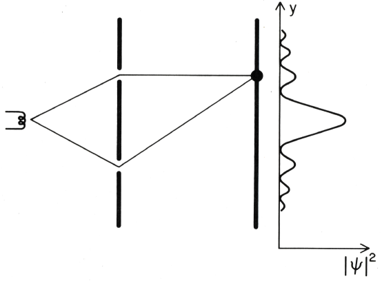
Figure 1: The two-slit experiment. An electron gun at right emits an electron traveling towards a screen with two slits, its progress in space recapitulating its evolution in time. When precise detections are made of an ensemble of such electrons at the screen it is not possible, because of interference, to assign a probability to the alternatives of whether an individual electron went through the upper slit or the lower slit. However, if the electron interacts with apparatus that measures which slit it passed through, then these alternatives decohere and probabilities can be assigned.

If we have measured which slit the electron went through, then the interference is destroyed, the sum rule obeyed, and we can meaningfully assign probabilities to these alternative histories.

A rule is thus needed in quantum theory to determine which sets of alternative histories are assigned probabilities and which are not. In Copenhagen quantum mechanics, the rule is that probabilities are assigned to histories of alternatives of a subsystem that are measured and not in general otherwise. It is the generalization of this rule that we seek in constructing a quantum mechanics of closed systems.

II.3 Probabilities for a Time Sequence of Measurements

To establish some notation, let us review in more detail the usual “Copenhagen” rules for the probabilities of time sequences of ideal measurements of a subsystem using the two-slit experiment of Figure 1 as an example.

Alternatives of the subsystem are represented by projection operators in the Hilbert space which describes it. Thus, in the two slit experiment, the alternative that the electron passed through the upper slit is represented by the projection operator

$$P_{U}=\Sigma_{s}\int_{U}d^{3}x\left|\vec{x},s\rangle\langle\vec{x},s\right|$$ (3)

where $|\vec{x},s\rangle$ is a localized state of the electron with spin component $s$, and the integral is over a volume around the upper slit. There is a similar projection operator $P_{L}$ for the alternative that the electron goes through the lower slit. These are exclusive alternatives and they are exhaustive. These properties, as well as the requirements of being projections, are represented by the relations

$$P_{L}^{2}=P^{2}_{U}=1\ ,\quad P_{L}P_{U}=0\ ,\quad P_{U}+P_{L}=I\,.$$ (4)

There is a similarly defined set of projection operators $\{P_{y_{k}}\}$ representing the alternative position intervals of arrival at the screen.

We can now state the rule for the joint probability that an electron initially in a state $|\psi(t_{0})\rangle$ at $t=t_{0}$ is determined by an ideal measurement at time $t_{1}$ to have passed through the upper slit and measured at time $t_{2}$ to arrive at point $y_{k}$ on the screen. If one likes, one can imagine the case when the electron is in a narrow wave packet in the horizontal direction with a velocity defined as sharply as possible consistent with the uncertainty principle. The joint probability is negligible unless $t_{1}$ and $t_{2}$ correspond to the times of flight to the slits and to the screen respectively.

The first step in calculating the joint probability is to evolve the state of the electron to the time $t_{1}$ of the first measurement

$$\bigl{|}\psi(t_{1})\bigr{\rangle}=e^{-iH(t_{1}-t_{0})/\hbar}\bigr{|}\psi(t_{0})\bigr{\rangle}\,.$$ (5)

The probability that the outcome of the measurement at time $t_{1}$ is that the electron passed through the upper slit is:

$$({\rm Probability\ of}\ U)=\left\|P_{U}\big{|}\psi(t_{1})\big{\rangle}\right\|^{2}$$ (6)

where $\|\cdot\|$ denotes the norm of a vector in Hilbert space. If the outcome was the upper slit, and the measurement was an “ideal” one, that disturbed the electron as little as possible in making its determination, then after the measurement the state vector is reduced to

$$\frac{P_{U}|\psi(t_{1})\rangle}{\|P_{U}|\psi(t_{1})\rangle\|}\,.$$ (7)

This is evolved to the time of the next measurement

$$|\psi(t_{2})\rangle=e^{-iH(t_{2}-t_{1})/\hbar}\frac{P_{U}|\psi(t_{1})\rangle}{\|P_{U}|\psi(t_{1})\rangle\|}\,.$$ (8)

The probability of being detected at time $t_{2}$ in one of a set of position intervals on the screen centered at $y_{k},k=1,2,\cdots$ given that the electron passed through the upper slit is

$$({\rm Probability\ of}\ y_{k}\ {\rm given}\ U)=\left\|P_{y_{k}}|\psi(t_{2})\rangle\right\|^{2}\,.$$ (9)

The joint probability that the electron is measured to have gone through the upper slit and is detected at $y_{k}$ is the product of the conditional probability (9) with the probability (6) that the electron passed through $U$. The latter factor cancels the denominator in (8) so that combining all of the above equations in this section, we have

$$({\rm Probability\ of}\ y_{k}\ {\rm and}\ U)=\left\|P_{y_{k}}e^{-iH(t_{2}-t_{1})/\hbar}P_{U}e^{-iH(t_{1}-t_{0})/\hbar}\big{|}\psi(t_{0})\big{\rangle}\right\|^{2}\,.$$ (10)

With Heisenberg picture projections this takes the even simpler form

$$({\rm Probability\ of}\ y_{k}\ {\rm and}\ U)=\left\|P_{y_{k}}(t_{2})P_{U}(t_{1})\ \big{|}\psi(t_{0})\rangle\right\|^{2}\,.$$ (11)

where, for example,

$$P_{U}(t)=e^{iHt/\hbar}P_{U}e^{-iHt/\hbar}\,.$$ (12)

The formula (11) is a compact and unified expression of the two laws of evolution that characterize the quantum mechanics of measured subsystems — unitary evolution in between measurements and reduction of the wave packet at a measurement. The important thing to remember about the expression (11) is that everything in it — projections, state vectors, and Hamiltonian — refer to the Hilbert space of a subsystem, in this example the Hilbert space of the electron that is measured.

Thus, in “Copenhagen” quantum mechanics, it is measurement that determines which histories can be assigned probabilities and formulae like (11) that determine what these probabilities are. As we mentioned, we cannot have such rules in the quantum mechanics of closed systems because there is no fundamental division of a closed system into measured subsystem and measuring apparatus and no fundamental reason for the closed system to contain classically behaving measuring apparatus in all circumstances. We need a more observer-independent, measurement-independent, classical domain-independent rule for which histories of a closed system can be assigned probabilities and what these probabilities are. The next section describes this rule.

II.4 Post-Everett Quantum Mechanics

It is easiest to introduce the rules of post-Everett quantum mechanics, by first making a simple assumption. That is to neglect gross quantum fluctuations in the geometry of spacetime, and assume a fixed background spacetime geometry which supplies a definite meaning to the notion of time. This is an excellent approximation on accessible scales for times later than $10^{-43}$ sec after the big bang. The familiar apparatus of Hilbert space, states, Hamiltonian, and other operators may then be applied to process of prediction. Indeed, in this context the quantum mechanics of cosmology is in no way distinguished from the quantum mechanics of a large isolated box, perhaps expanding, but containing both the observed and its observers (if any).

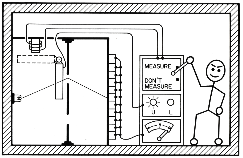
Figure 2: A model closed quantum system. At one fundamental level of description this system consists of a large number of electrons, nucleons, and excitations of the electromagnetic field. However, the initial state of the system is such that at a coarser level description it contains an observer together with the necessary apparatus for carrying out a two-slit experiment. Alternatives for the system include whether the “system” contains a two-slit experiment or not, whether it contains an observer or not, whether the observer measured which slit the electron passed through or did not, whether the electron passed through the upper or lower slit, the alternative positions of arrival of the electron at the screen, the alternative arrival positions registered by the apparatus, the registration of these in the brain of the observer, etc., etc., etc. Each exhaustive set of exclusive alternatives is represented by an exhaustive set of orthogonal projection operators on the Hilbert space of the closed system. Time sequences of such sets of alternatives describe sets of alternative coarse-grained histories of the closed system. Quantum theory assigns probabilities to the individual alternative histories in such a set when there is negligible quantum mechanical interference between them, that is, when the set of histories decoheres.

A set of alternative histories for such a closed system is specified by giving exhaustive sets of exclusive alternatives at a sequence of times. Consider a model closed system with a quantity of matter initially in a pure state that can be described as an observer and two-slit experiment, with appropriate apparatus for producing the electrons, detecting which slit they passed through, and measuring their position of arrival on the screen (Figure 2). Some alternatives for the whole system are:

1. Whether or not the observer decided to measure which slit the electron went through.

2. Whether the electron went through the upper or lower slit.

3. The alternative positions, $y_{1},\cdots,y_{N}$, that the electron could have arrived at the screen.

These sets of alternatives at a sequence of times define a set of histories whose characteristic branching structure is shown in Figure 3. An individual history in the set is specified by some particular sequence of alternatives, e.g. measured, upper, $y_{9}$.

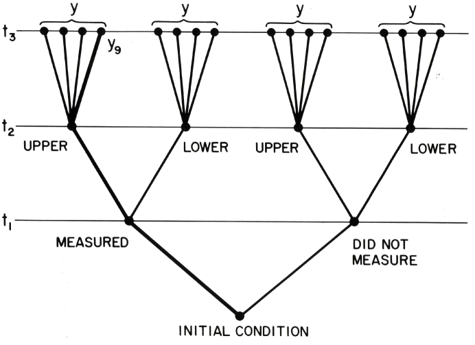
Figure 3: Branching structure of a set of alternative histories. This figure illustrates the set of alternative histories for the model closed system of Figure 2 defined by the alternatives of whether the observer decided to measure or did not decide to measure which slit the electron went through at time $t_{1}$, whether the electron went through the upper slit or through the lower slit at time $t_{2}$, and the alternative positions of arrival at the screen at time $t_{3}$. A single branch corresponding to the alternatives that the measurement was carried out, the electron went through the upper slit, and arrived at point $y_{9}$ on the screen is illustrated by the heavy line.
The illustrated set of histories does not decohere because there is significant quantum mechanical interference between the branch where no measurement was carried out and the electron went through the upper slit and the similar branch where it went through the lower slit. A related set of histories that does decohere can be obtained by replacing the alternatives at time $t_{2}$ by the following set of three alternatives: (a record of the decision shows a measurement was initiated and the electron went through the upper slit); (a record of the decision shows a measurement was initiated and the electron went through the lower slit); (a record of the decision shows that the measurement was not initiated). The vanishing of the interference between the alternative values of the record and the alternative configurations of apparatus ensures the decoherence of this set of alternative histories.

Many other sets of alternative histories are possible for the closed system. For example, we could have included alternatives describing the readouts of the apparatus that detects the position that the electron arrived on the screen. If the initial condition corresponded to a good experiment there should be a high correlation between these alternatives and the position that the electron arrives at the screen. We could discuss alternatives corresponding to thoughts in the observer’s brain, or to the individual positions of the atoms in the apparatus, or to the possibilities that these atoms reassemble in some completely different configuration. There are a vast number of possibilities.

Characteristically the alternatives that are of use to us as observers are very coarse grained, distinguishing only very few of the degrees of freedom of a large closed system and distinguishing these only at a small subset of the possible times. This is especially true if we recall that our box with observer and two-slit experiment is only an idealized model. The most general closed system is the universe itself, and, as we shall show, the only realistic closed systems are of cosmological dimensions. Certainly, we utilize only very, very coarse-grained descriptions of the universe as a whole.

Let us now state the rules that determine which coarse-grained sets of histories of a closed system may be assigned probabilities and what those probabilities are. The essence of the rules can be found in the work of Bob Griffiths Gri84 . The general framework was extended by Roland Omnès Omnsum and was independently, but later, arrived at by Murray Gell-Mann and the author GH90a . The idea is simple: The obstacle to assigning probabilites is the failure of the probability sum rules due to quantum interference. Probabilities can be therefore be assigned to just those sets of alternative histories of a closed system for which there is negligible interference between the individual histories in the set as a consequence of the particular initial state the closed system has, and for which, therefore, all probability sum rules are satisfied. Let us now give this idea a precise expression.

Sets of alternatives at one moment of time, for example the set of alternative position intervals $\{y_{k}\}$ at which the electron might arrive at the screen, are represented by exhaustive sets of orthogonal projection operators. Employing the Heisenberg picture these can be denoted $\{P_{\alpha}(t)\}$ where $\alpha$ ranges over a set of integers and $t$ denotes the time at which the alternatives are defined. A particular alternative corresponds to a particular $\alpha$. For example, in the two-slit experiment, $\alpha=9$ might be the alternative that the electron arrives in the position interval $y_{9}$ at the screen. $P_{9}(t)$ would be a projection on that interval at time $t$. Sets of alternative histories are defined by giving sequences of sets of alternatives at definite moments of time $t_{1},\dots,t_{n}$ We denote the sequence of such sets by $\{P^{1}_{\alpha_{1}}(t_{1})\}\ ,\{P^{2}_{\alpha_{2}}(t_{2})\},\cdots,\{P^{n}_{\alpha_{n}}(t_{n})\}$. The sets are in general different at different times. For example in the two-slit experiment $\{P^{2}_{\alpha_{2}}(t_{2})\}$ could be the set which distinguishes whether the electron went through the upper slit or the lower slit at time $t_{2}$, while $\{P^{3}_{\alpha_{3}}(t_{3})\}$ might distinguish various positions of arrival at the final screen at time $t_{3}$. More generally the $\{P^{k}_{\alpha_{k}}(t_{k})\}$ might be projections onto ranges of momentum or the ranges of the eigenvalues of any other Hermitian operator at time $t_{k}$. The superscript $k$ distinguishes these different sets in a sequence. Each set of $P$’s satisfies

$$\sum\nolimits_{\alpha_{k}}P^{k}_{\alpha_{k}}(t_{k})=I\ ,\quad P^{k}_{\alpha_{k}}(t_{k})P^{k}_{\alpha^{\prime}_{k}}(t_{k})=\delta_{\alpha_{k}\alpha^{\prime}_{k}}P^{k}_{\alpha_{k}}(t_{k})\,,$$ (13)

showing that they represent an exhaustive set of exclusive alternatives. An individual history corresponds to a particular sequence $(\alpha_{1},\cdots,\alpha_{n})\equiv\alpha$ and, for each history, there is a corresponding chain of time ordered projection operators

$$C_{\alpha}\equiv P^{n}_{\alpha_{n}}(t_{n})\cdots P^{1}_{\alpha_{1}}(t_{1})\,.$$ (14)

Such histories are said to be coarse-grained when, as is typically the case, the $P$’s are not projections onto a basis (a complete set of states) and when there is not a set of $P$’s at each and every time.

As an example, in the two-slit experiment illustrated in Figure 2 consider the history in which the observer decided at time $t_{1}$ to measure which slit the electron goes through, in which the electron goes through the upper slit at time $t_{2}$, and arrives at the screen in position interval $y_{9}$ at time $t_{3}$. This would be represented by the chain

$$P^{3}_{y_{9}}(t_{3})P^{2}_{U}(t_{2})P^{1}_{\rm meas}(t_{1})$$ (15)

in an obvious notation. Evidently this is a very coarse-grained history, involving only three times and ignoring most of the coordinates of the particles that make up the apparatus in the closed system. As far as the description of histories is concerned, the only difference between this situation and that of the “Copenhagen” quantum mechanics of measured subsystems is the following: The sets of operators $\{P^{k}_{\alpha_{k}}(t_{k})\}$ defining alternatives for the closed system act on the Hilbert space of the closed system that includes the variables describing any apparatus, observers, their constituent particles, and anything else. The operators defining alternatives in Copenhagen quantum mechanics act only on the Hilbert space of the measured subsystem.

When the initial state is pure, it can be resolved into branches corresponding to the individual members of any set of alternative histories. (The generalization to an impure initial density matrix is not difficult and will be discussed in the next section.) Denote the initial state by $|\Psi\rangle$ in the Heisenberg picture. Then

$$|\Psi\rangle=\sum\nolimits_{\alpha}C_{\alpha}|\Psi\rangle=\sum\limits_{\alpha_{1},\cdots,\alpha_{n}}P^{n}_{\alpha_{n}}(t_{n})\cdots P^{1}_{\alpha_{1}}(t_{1})|\Psi\rangle\,.$$ (16)

This identity follows by applying the first of (13) to all the sums over $\alpha_{k}$ in turn. The vector

$$C_{\alpha}|\Psi\rangle$$ (17)

is the branch of $|\Psi\rangle$ corresponding to the individual history $\alpha$ and (16) is the resolution of the initial state into branches.

When the branches corresponding to a set of alternative histories are sufficiently orthogonal, the set of histories is said to decohere. More precisely a set of histories decoheres when

$$\langle\Psi|C^{\dagger}_{\alpha}C_{\alpha\prime}|\Psi\rangle\approx 0\ ,\quad{\rm for\ }\ \ \alpha\not=\alpha^{\prime}\,.$$ (18)

Here, two histories $\alpha=(\alpha_{1}\cdots\alpha_{n})$ and $\alpha^{\prime}=(\alpha^{\prime}_{1}\cdots\alpha^{\prime}_{n})$ are equal when all the $\alpha_{k}=\alpha^{\prime}_{k}$ and are unequal when any $\alpha_{k}\neq\alpha^{\prime}_{k}$. We shall return to the standard with which decoherence should be enforced, but first let us examine its meaning and consequences.

Decoherence means the absence of quantum mechanical interference between the individual histories of a coarse-grained set. Probabilities can be assigned to the individual histories in a decoherent set of alternative histories because decoherence implies the probability sum rules necessary for a consistent assignment. The probability of an individual history $\alpha$ is

$$p(\alpha)=\left\|C_{\alpha}|\Psi\rangle\right\|^{2}\,.$$ (19)

To see how decoherence implies the probability sum rules, let us consider an example in which there are just three sets of alternatives at times $t_{1},t_{2}$, and $t_{3}$. A typical sum rule might be

$$\sum\nolimits_{\alpha_{2}}p\left(\alpha_{3},\alpha_{2},\alpha_{1}\right)=p\left(\alpha_{3},\alpha_{1}\right)\,.$$ (20)

We shall now show that (18) and (19) imply (20). To do that write out the left hand side of (20) using (19) and suppress the time labels for compactness.

$$\sum\nolimits_{\alpha_{2}}p\left(\alpha_{3},\alpha_{2},\alpha_{1}\right)=\sum\nolimits_{\alpha_{2}}\bigl{\langle}\Psi|P^{1}_{\alpha_{1}}P^{2}_{\alpha_{2}}P^{3}_{\alpha_{3}}P^{3}_{\alpha_{3}}P^{2}_{\alpha_{2}}P^{1}_{\alpha_{1}}|\Psi\bigr{\rangle}\,.$$ (21)

Decoherence means that the sum on the right hand side of (21) can be written with negligible error as

$$\sum\nolimits_{\alpha_{2}}p\left(\alpha_{3},\alpha_{2},\alpha_{1}\right)\approx\sum\nolimits_{\alpha^{\prime}_{2}\alpha_{2}}\bigl{\langle}\Psi|P^{1}_{\alpha_{1}}P^{2}_{\alpha^{\prime}_{2}}P^{3}_{\alpha_{3}}P^{3}_{\alpha_{3}}P^{2}_{\alpha_{2}}P^{1}_{\alpha_{1}}|\Psi\bigr{\rangle}\,.$$ (22)

the extra terms in the sum being vanishingly small. But now, applying the first of (13) we see

$$\sum\nolimits_{\alpha_{2}}p\left(\alpha_{3},\alpha_{2},\alpha_{1}\right)\approx\bigl{\langle}\Psi|P^{1}_{\alpha_{1}}P^{3}_{\alpha_{3}}P^{3}_{\alpha_{3}}P^{1}_{\alpha_{1}}|\Psi\bigr{\rangle}=p\left(\alpha_{3},\alpha_{1}\right)$$ (23)

so that the sum rule (20) is satisfied.

Given an initial state $|\Psi\rangle$ and a Hamiltonian $H$, one could, in principle, identify all possible sets of decohering histories. Among these will be the exactly decohering sets where the orthogonality of the branches is exact. Indeed, trivial examples can be supplied by resolving $|\Psi\rangle$ into a sum of orthogonal vectors $|\Psi_{\alpha_{1}}\rangle$, resolving these into vectors $|\Psi_{\alpha_{2}\alpha_{1}}\rangle$ such that the whole set is orthogonal, and so on for $n$ steps. The result is a resolution of $|\Psi\rangle$ into exactly orthogonal branches $|\Psi_{\alpha_{n}\cdots\alpha_{1}}\rangle$. By introducing suitable projections and assigning them times $t_{1},\cdots,t_{n}$, this set of branches could be represented in the form (16) giving an exactly decoherent set of histories. Indeed, if the $|\Psi_{\alpha_{n}\cdots\alpha_{1}}\rangle$ are not complete, there are typically many different choices of projections that will do this.

Exactly decoherent sets of histories are thus not difficult to achieve mathematically, but such artifices will not, in general, have a simple description in terms of fundamental fields nor any connection, for example, with the quasiclassical domain of familiar experience. For this reason sets of histories that approximately decohere are also of interest. As we will argue in the next two sections, realistic mechanisms lead to the decoherence of a set of histories describing a quasiclassical domain that decohere to an excellent approximation as measured by DH92

$$\left|\left\langle\Psi\right|C^{\dagger}_{\alpha}C_{\alpha^{\prime}}\left|\Psi\right\rangle\right|<<<\left\|C_{\alpha}\left|\Psi\bigl{\rangle}\right\|\cdot\bigl{\|}C_{\alpha^{\prime}}\right|\Psi\bigr{\rangle}\bigr{\|},\quad{\rm for}\ \alpha^{\prime}\not=\alpha\,.$$ (24)

When the decoherence condition (18) is only approximately enforced, the probability sum rules such as (20) will be only approximately obeyed. However, as discussed earlier, probabilities for single systems are meaningful up to the standard they are used. Approximate probabilities for which the sum rules are satisfied to a comparable standard may therefore also be employed in the process of prediction. When we speak of approximate decoherence and approximate probabilities we mean decoherence achieved and probability sum rules satisfied beyond any standard that might be conceivably contemplated for the accuracy of prediction and the comparison of theory with experiment.

We thus have a picture of the collection of all possible sets of alternative coarse-grained histories of a closed system. Within that collection are the sets of histories that decohere and are assigned approximate probabilities by quantum theory. Within that collection are the sets of histories describing the quasiclassical domain of utility for everyday experience as we shall describe in Section II.7.

Decoherent sets of alternative histories of the universe are what can be utilized in the process of prediction in quantum mechanics, for they may be assigned probabilities. Decoherence thus generalizes and replaces the notion of “measurement”, which served this role in the Copenhagen interpretations. Decoherence is a more precise, more objective, more observer-independent idea and gives a definite meaning to Everett’s branches. For example, if their associated histories decohere, we may assign probabilities to various values of reasonable scale density fluctuations in the early universe whether or not anything like a “measurement” was carried out on them and certainly whether or not there was an “observer” to do it.

II.5 The Origins of Decoherence in Our Universe

What are the features of coarse-grained sets of histories that decohere in our universe? In seeking to answer this question it is important to keep in mind the basic aspects of the theoretical framework on which decoherence depends. Decoherence of a set of alternative histories is not a property of their operators alone. It depends on the relations of those operators to the initial state $|\Psi\rangle$, the Hamiltonian $H$, and the fundamental fields. Given these, we could, in principle, compute which sets of alternative histories decohere.

We are not likely to carry out a computation of all decohering sets of alternative histories for the universe, described in terms of the fundamental fields, any time in the near future, if ever. It is therefore important to investigate specific mechanisms by which decoherence occurs. Let us begin with a very simple model due to Joos and Zeh JZ85 in its essential features. We consider the two-slit example again, but this time suppose that in the neighborhood of the slits there is a gas of photons or other light particles colliding with the electrons. Physically it is easy to see what happens, the random uncorrelated collisions carry away delicate phase correlations between the beams even if the trajectories of the electrons are not affected much. The interference pattern is destroyed and it is possible to assign probabilities to whether the electron went through the upper slit or the lower slit.

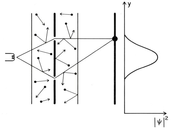
Figure 4: The two-slit experiment with an interacting gas. Near the slits light particles of a gas collide with the electrons. Even if the collisions do not affect the trajectories of the electrons very much they can still carry away the phase correlations between the histories in which the electron arrived at point $y_{k}$ on the screen by passing through the upper slit and that in which it arrived at the same point by passing through the lower slit. A coarse graining that consisted only of these two alternative histories of the electron would approximately decohere as a consequence of the interactions with the gas given adequate density, cross-section, etc. Interference is destroyed and probabilities can be assigned to these alternative histories of the electron in a way that they could not be if the gas were not present (cf. Fig. 1). The lost phase information is still available in correlations between states of the gas and states of the electron. The alternative histories of the electron would not decohere in a coarse graining that included both the histories of the electron and operators that were sensitive to the correlations between the electrons and the gas.
This model illustrates a widely occurring mechanism by which certain types of coarse-grained sets of alternative histories decohere in the universe.

Let us see how this picture in words is given precise meaning in mathematics. Initially, suppose the state of the entire system is a state of the electron $|\psi>$ and $N$ distinguishable “photons” in states $|\varphi_{1}\rangle$, $|\varphi_{2}\rangle$, etc., viz.

$$|\Psi\rangle=|\psi\rangle|\varphi_{1}\rangle|\varphi_{2}>\cdots|\varphi_{N}\rangle\,.$$ (25)

The electron state $|\psi\rangle$ is a coherent superposition of a state in which the electron passes through the upper slit $|U\rangle$ and the lower slit $|L\rangle$. Explicitly:

$$|\psi\rangle=\alpha|U\rangle+\beta|L\rangle\,.$$ (26)

Both states are wave packets in horizontal position, $x$, so that position in $x$ recapitulates history in time. We now ask whether the history where the electron passes through the upper slit and arrives at a detector defining an interval $y_{k}$ on the screen, decoheres from that in which it passes through the lower slit and arrives the interval $y_{k}$, as a consequence of the initial condition of this “universe”. That is, as in Section 4, we ask whether the two branches

$$P_{y_{k}}(t_{2})P_{U}(t_{1})|\Psi\rangle\quad,\quad P_{y_{k}}(t_{2})P_{L}(t_{1})|\Psi\rangle$$ (27)

are nearly orthogonal, the times of the projections being those for the nearly classical motion in $x$. We work this out in the Schrödinger picture where the initial state evolves, and the projections on the electron’s position are applied to it at the appropriate times.

Collisions occur, but the states $|U\rangle$ and $|L\rangle$ are left more or less undisturbed. The states of the “photons” are, of course, significantly affected. If the photons are dilute enough to be scattered only once by the electron in its time to traverse the gas, the two branches (27) will be approximately

$$\alpha P_{y_{k}}|U\rangle S_{U}|\varphi_{1}\rangle S_{U}|\varphi_{2}\rangle\cdots S_{U}|\varphi_{N}\rangle\,,$$ (28a)

and

$$\beta\ P_{y_{k}}|L\rangle S_{L}|\varphi_{1}\rangle S_{L}|\varphi_{2}\rangle\cdots S_{L}|\varphi_{N}\rangle\,.$$ (28b)

Here, $S_{U}$ and $S_{L}$ are the scattering matrices from an electron in the vicinity of the upper slit and the lower slit respectively. The two branches in (28) decohere because the states of the “photons” are nearly orthogonal. The overlap of the branches is proportional to

$$\langle\varphi_{1}|S^{\dagger}_{U}S_{L}|\varphi_{1}\rangle\langle\varphi_{2}|S^{\dagger}_{U}S_{L}|\varphi_{2}\rangle\cdots\langle\varphi_{N}|S^{\dagger}_{U}S_{L}\ |\varphi_{N}\rangle\,.$$ (29)

Now, the $S$-matrices for scattering off an electron at the upper position or the lower position can be connected to that of an electron at the origin by a translation

$$S_{U} = \exp(-i\vec{k}\cdot{\vec{x}}_{U})S\ \exp(+i{\vec{k}}\cdot{\vec{x}}_{U})\,,$$ (30a)

$$S_{L} = \exp(-i{\vec{k}}\cdot{\vec{x}}_{L})S\ \exp(+i{\vec{k}}\cdot{\vec{x}}_{L})\,.$$ (30b)

Here, $\hbar{\vec{k}}$ is the momentum of a photon, ${\vec{x}}_{U}$ and ${\vec{x}}_{L}$ are the positions of the slits and $S$ is the scattering matrix from an electron at the origin.

$$\langle{\vec{k}}^{\prime}|S|{\vec{k}}\rangle=\delta^{(3)}\bigl{(}{\vec{k}}-{\vec{k}}^{\prime}\bigr{)}+\frac{i}{2\pi\omega_{k}}f\bigl{(}{\vec{k}},{\vec{k}}^{\prime}\bigr{)}\delta\bigl{(}{\omega_{k}}-\omega^{\prime}_{k}\bigr{)}\,,$$ (31)

where $f$ is the scattering amplitude and $\omega_{k}=|{\vec{k}}|$.

Consider the case where all the photons are in plane wave states in an interaction volume $V$, all having the same energy $\hbar\omega$, but with random orientations for their momenta. Suppose further that the energy is low so that the electron is not much disturbed by a scattering and low enough so the wavelength is much longer than the separation between the slits, $k|{\vec{x}}_{U}-{\vec{x}}_{L}|<<1$. It is then possible to work out the overlap. The answer according to Joos and Zeh JZ85 is

$$\left(1-\frac{(k|{\vec{x}}_{U}-{\vec{x}}_{L}|)^{2}}{8\pi^{2}V^{2/3}}\sigma\right)^{N}$$ (32)

where $\sigma$ is the effective scattering cross section. Even if $\sigma$ is small, as $N$ becomes large this tends to zero. In this way decoherence becomes a quantitative phenomenon.

What such models convincingly show is that decoherence is frequent and widespread in the universe. Joos and Zeh calculate that a superposition of two positions of a grain of dust, 1mm apart, is decohered simply by the scattering of the cosmic background radiation on the time-scale of a nanosecond. The existence of such mechanisms means that the only realistic isolated systems are of cosmological dimensions. So widespread is this kind of phenomena with the initial condition and dynamics of our universe, that we may meaningfully speak of habitually decohering variables such as the center of mass positions of massive bodies.

II.6 The Copenhagen Approximation

What is the relation of the familiar Copenhagen quantum mechanics described in Section II.3 to the more general “post-Everett” quantum mechanics of closed systems described in Sections II.4 and II.5? Copenhagen quantum mechanics predicts the probabilities of the histories of measured subsystems. Measurement situations may be described in a closed system that contains both measured subsystem and measuring apparatus.. measurement In a typical measurement situation the values of a variable not normally decohering become correlated with alternatives of the apparatus that decohere because of its interactions with the rest of the closed system. The correlation means that the measured alternatives decohere because the alternatives of the apparatus decohere.

The recovery of the Copenhagen rule for when probabilities may be assigned is immediate. Measured quantities are correlated with decohering histories. Decohering histories can be assigned probabilities. Thus in the two-slit experiment (Figure 1), when the electron interacts with an apparatus that determines which slit it passed through, it is the decoherence of the alternative configurations of the apparatus that register this determination that enables probabilities to be assigned to the alternatives for electron.

There is nothing incorrect about Copenhagen quantum mechanics. Neither is it, in any sense, opposed to the post-Everett formulation of the quantum mechanics of closed systems. It is an approximation to the more general framework appropriate in the special cases of measurement situations and when the decoherence of alternative configurations of the apparatus may be idealized as exact and instantaneous. However, while measurement situations imply decoherence, they are only special cases of decohering histories. Probabilities may be assigned to alternative positions of the moon and to alternative values of density fluctuations near the big bang in a universe in which these alternatives decohere, whether or not they were participants in a measurement situation and certainly whether or not there was an observer registering their values.

II.7 Quasiclassical Domains

As observers of the universe, we deal with coarse-grained histories that reflect our own limited sensory perceptions, extended by instruments, communication and records but in the end characterized by a large amount of ignorance. Yet, we have the impression that the universe exhibits a much finer-grained set of histories, independent of us, defining an always decohering “quasiclassical domain”, to which our senses are adapted, but deal with only a small part of it. If we are preparing for a journey into a yet unseen part of the universe, we do not believe that we need to equip ourselves with spacesuits having detectors sensitive, say, to coherent superpositions of position or other unfamiliar quantum variables. We expect that the familiar quasiclassical variables will decohere and be approximately correlated in time by classical deterministic laws in any new part of the universe we may visit just as they are here and now.

In a generalization of quantum mechanics which does not posit the existence of a classical domain, the domain of applicability of classical physics must be explained. For a quantum mechanical system to exhibit classical behavior there must be some restriction on its state and some coarseness in how it is described. This is clearly illustrated in the quantum mechanics of a single particle. Ehrenfest’s theorem shows that generally

$$M\frac{d^{2}\langle x\rangle}{dt^{2}}=\left\langle-\frac{\partial V}{\partial x}\right\rangle\,.$$ (33)

However, only for special states, typically narrow wave packets, will this become an equation of motion for $\langle x\rangle$ of the form

$$M\frac{d^{2}\langle x\rangle}{dt^{2}}=-\frac{\partial V(\langle x\rangle)}{\partial x}\,.$$ (34)

For such special states, successive observations of position in time will exhibit the classical correlations predicted by the equation of motion (34) provided that these observations are coarse enough so that the properties of the state which allow (34) to replace the general relation (33) are not affected by these observations. An exact determination of position, for example, would yield a completely delocalized wave packet an instant later and (34) would no longer be a good approximation to (33). Thus, even for large systems, and in particular for the universe as a whole, we can expect classical behavior only for certain initial states and then only when a sufficiently coarse grained description is used.

If classical behavior is in general a consequence only of a certain class of states in quantum mechanics, then, as a particular case, we can expect to have classical spacetime only for certain states in quantum gravity. The classical spacetime geometry we see all about us in the late universe is not a property of every state in a theory where geometry fluctuates quantum mechanically. Rather, it is traceable fundamentally to restrictions on the initial condition. Such restrictions are likely to be generous in that, as in the single particle case, many different states will exhibit classical features. The existence of classical spacetime and the applicability of classical physics are thus not likely to be very restrictive conditions on constructing a theory of the initial condition. Fundamentally, however, the existence of one or more quasiclassical domains of the universe must be a prediction of any successful theory of its initial condition and dynamics, and thus an important problem for quantum cosmology.

Roughly speaking, a quasiclassical domain should be a set of alternative histories that decoheres according to a realistic principle of decoherence, that is maximally refined consistent with that notion of decoherence, and whose individual histories exhibit as much as possible patterns of classical correlation in time. To make the question of the existence of one or more quasiclassical domains into a calculable question in quantum cosmology we need measures of how close a set of histories comes to constituting a “quasiclassical domain”. A quasiclassical domain cannot be a completely fine-grained description for then it would not decohere. It cannot consist entirely of a few “classical variables” repeated over and over because sometimes we may measure something highly quantum mechanical. These variables cannot be always correlated in time by classical laws because sometimes quantum mechanical phenomena cause deviations from classical physics. We need measures for maximality and classicality GH90a .

It is possible to give crude arguments for the type of habitually decohering operators we expect to occur over and over again in a set of histories defining a quasiclassical domain GH90a . Such habitually decohering operators are called “quasiclassical operators”. In the earliest instants of the universe the operators defining spacetime on scales well above the Planck scale emerge from the quantum fog as quasiclassical. Any theory of the initial condition that does not imply this is simply inconsistent with observation in a manifest way. A background spacetime is thus defined and conservation laws arising from its symmetries have meaning. Then, where there are suitable conditions of low temperature, density, etc., various sorts of hydrodynamic variables may emerge as quasiclassical operators. These are integrals over suitably small volumes of densities of conserved or nearly conserved quantities. Examples are densities of energy, momentum, baryon number, and, in later epochs, nuclei, and even chemical species. The sizes of the volumes are limited above by maximality and are limited below by classicality because they require sufficient “inertia” resulting from their approximate conservation to enable them to resist deviations from predictability caused by their interactions with one another, by quantum spreading, and by the quantum and statistical fluctuations resulting from interactions with the rest of the universe that accomplish decoherence GH90a . Suitable integrals of densities of approximately conserved quantities are thus candidates for habitually decohering quasiclassical operators. These “hydrodynamic variables” are among the principle variables of classical physics.

It would be in such ways that the classical domain of familiar experience could be an emergent property of the fundamental description of the universe, not generally in quantum mechanics, but as a consequence of our specific initial condition and the Hamiltonian describing evolution. Whether a closed system exhibits a quasiclassical domain, and, indeed, whether it exhibits more than one essentially inequivalent domain, thus become calculable questions in the quantum mechanics of closed systems.

The founders of quantum mechanics were right in pointing out that something external to the framework of wave function and the Schrödinger equation is needed to interpret the theory. But it is not a postulated classical domain to which quantum mechanics does not apply. Rather it is the initial condition of the universe that, together with the action function of the elementary particles and the throws of the quantum dice since the beginning, is the likely origin of quasiclassical domain(s) within quantum theory itself.

III Decoherence in General, Decoherence in Particular,
and the Emergence of Classical Behavior

III.1 A More General Formulation of the Quantum Mechanics of Closed Systems

The basic ideas of post-Everett quantum mechanics were introduced in the preceding section. We can briefly recapitulate these as follows: The most general predictions of quantum mechanics are the probabilities of alternative coarse-grained histories of a closed system in an exhaustive set of such histories. Not every set of coarse-grained histories can be assigned probabilities because of quantum mechanical interference and the consequent failure of probability sum rules. Rather, probabilities are predicted only for those decohering sets of histories for which interference between the individual members is negligible as a consequence of the system’s initial condition and Hamiltonian and the probability sum rules therefore obeyed. Among the decohering sets implied by the initial condition of our universe are those constituting the quasiclassical domain of familiar experience.

The discussion of Section II was oversimplified in several respects. For example, we restricted attention to pure initial states, considered only sets of alternatives at definite moments of time, considered only sets of alternatives at any one moment that were independent of alternatives at other moments of time, and assumed a fixed background spacetime. None of these restrictions is realistic. In the rest of these lectures we shall be pursuing the necessary generalizations needed for a more realistic formulation. In this section we develop a more general framework still assuming a fixed spacetime geometry that supplies a meaning to time and still restricting attention to alternatives at definite moments of time.

III.1.1 Fine-Grained and Coarse-Grained Histories

We consider a closed quantum mechanical system described by a Hilbert space ${\cal H}$. As described in Section II, a set of alternatives at one moment of time is described by a set of orthogonal Heisenberg projection operators $\{P^{k}_{\alpha_{k}}(t_{k})\}$ satisfying (13). The operators corresponding to the same alternatives at different times are related by unitary evolution

$$P^{k}_{\alpha_{k}}(t_{k})=e^{iHt_{k}/\hbar}\,P^{k}_{\alpha_{k}}(0)\,e^{-iHt_{k}/\hbar}\,.$$ (35)

Sequences of such sets of alternatives at, say, times $t_{1},\cdots,t_{n}$ define a set of alternative histories for the closed system. The individual histories in such a set consist of particular chains of alternatives $\alpha=(\alpha_{1},\cdots,\alpha_{n})$ and are represented by the corresponding chains of projection operators, $C_{\alpha}$, as in (14).

Sets of histories described in this way are in general coarse-grained because they do not define alternatives at each and every time and because the projections specifying the alternatives are not onto complete sets of states (one-dimensional projections onto a basis) at the times when they are defined. The fine-grained sets of histories on a time interval $[0,T]$ are defined by giving sets of one-dimensional projections at each time and so are represented by continuous products of one-dimensional projections. These are the most refined descriptions of the quantum mechanical system possible. There are many different sets of fine-grained histories. A simple example of fine- and coarse-grained histories occurs when ${\cal H}$ is the space of square integrable functions on a configuration space of generalized coordinates $\{q^{i}\}$ (for example, modes of field configurations on a spacelike surface). Exhaustive sets of exclusive coordinate ranges at a sequence of times define a set of coarse-grained histories. If the ranges are made smaller and smaller and more and more dense in time, these increasingly fine-grained histories come closer and closer to representing continuous paths $q^{i}(t)$ on the interval $[0,T]$. These paths are the starting point for a sum-over-histories formulation of quantum mechanics. Operators $C_{\alpha}$ corresponding to the individual paths themselves do not exist because there are no exactly localized states in ${\cal H}$, but the $C_{\alpha}$ on the finer- and finer-grained histories described above represent them in the familiar way continuous spectra are handled in quantum mechanics.

A set of alternatives at one moment of time may be further coarse-grained by taking the union of alternatives corresponding to the logical operation “or”. If $P_{a}$ and $P_{b}$ are the projections corresponding to alternatives “$a$” and “$b$” respectively, then $P_{a}+P_{b}$ is the projection corresponding to the alternative “$a$ or $b$”. This is the simplest example of an operation of coarse-graining. This operation “or” can be applied to histories. If $C_{\alpha}$ is the operator representing one history in a coarse-grained set, and $C_{\beta}$ is another, then the coarser grained alternative in which the system follows either history $\alpha$ or history $\beta$ is represented by

$$C_{\alpha\ {\rm or}\ \beta}=C_{\alpha}+C_{\beta}\,.$$ (36)

Thus, if $\{c_{\alpha}\}$ is a set of alternative histories for the closed system defined by sequences of alternatives at definite moments of time, then the general notion of a coarse graining of this set of histories is a partition of the $\{c_{\alpha}\}$ into exclusive classes $\{c_{\bar{\alpha}}\}$. The classes are the individual histories in the coarser grained set and are represented by operators, called class operators, that are sums of the chains of the constituent projections in the finer-grained set:

$$C_{\bar{\alpha}}=\sum\limits_{\alpha\epsilon\bar{\alpha}}C_{\alpha}\,.$$ (37)

When the $C_{\alpha}$ are chains of projections we have:

$$C_{\bar{\alpha}}=\sum\limits_{(\alpha_{1},\cdots,\alpha_{n})\epsilon\bar{\alpha}}P^{n}_{\alpha_{n}}(t_{n})\cdots P^{1}_{\alpha_{1}}(t_{1})\,.$$ (38)

These $\{C_{\bar{\alpha}}\}$ may sometimes be representable as chains of projections (as when the sum is over alternatives at just one time). However, they will not generally be chains of projections. The general operator corresponding to a coarse-grained history will thus be a class operator of the form (38).

In a similar manner one can define operations of fine-graining. For example, introducing a set of alternatives at a time when there was none before is an operation of fine-graining as is splitting the projections of an existing set at one time into more mutually orthogonal ones. Continued fine-graining would eventually result in a completely fine-grained set of histories. All coarse-grained sets of histories are therefore coarse grainings of at least one fine-grained set.

Sets of histories are partially ordered by the operations of coarse graining and fine graining. For any pair of sets of histories, the least coarse-grained set, of which they are both fine grainings, can be defined. However, there is not, in general, a unique fine-grained set of which they are both a coarse graining. There is an operation of “join” but not of “meet”.

So far we have considered histories defined by sets of alternatives at sequences of times that are independent of one another. For realistic situations we are interested in sets of histories in which (assuming causality) the set of alternatives and their times are dependent on the particular alternatives and particular times that define the history at earlier times. Such sets of histories are said to be branch dependent. A more complete notation would be to write:

$$P^{n}_{\alpha_{n}}\left(t_{n};\alpha_{n-1},t_{n-1},\cdots,\alpha_{1},t_{1}\right)\,P^{n-1}_{\alpha_{n-1}}\left(t_{n-1};\alpha_{n-2},t_{n-2},\cdots,\alpha_{1},t_{1}\right)\cdots P^{1}_{\alpha_{1}}(t_{1})\,,$$ (39)

for histories represented by chains of such projections. Here $\{P^{k}_{\alpha_{k}}(t_{k};\alpha_{k-1},t_{k-1},\cdots$, $\alpha_{1},t_{1})\}$ are an exhaustive set of orthogonal projection operators as $\alpha_{k}$ varies, keeping $\alpha_{k-1},t_{k-1},\cdots,\alpha_{1},t_{1}$ fixed. Nothing more than replacing chains in (38) by (39) is needed to complete the generalization to branch dependent histories.

Branch dependence is important, for example, in describing realistic quasiclassical domains because past events may determine what is a suitable quasiclassical variable. For instance, if a quantum fluctuation gets amplified so that a galaxy condenses in one branch and no such condensation occurs in other branches, then what are suitable quasiclassical variables in the region where the galaxy would form is branch dependent. While branch dependent sets of histories are clearly important for a description of realistic quasiclassical domains, we shall not make much use of them in these lectures devoted to general frameworks and frequently use the notation in (38) as an abbreviation for the more precise (39).

III.1.2 The Decoherence Functional

Quantum mechanical interference between individual histories in a coarse-grained set is measured by a decoherence functional. This is a complex-valued functional on pairs of histories in a coarse-grained set depending on the initial condition of the closed system. If $c_{\alpha^{\prime}}$ and $c_{\alpha}$ are a pair of histories, $C_{\alpha^{\prime}},C_{\alpha}$ are the corresponding operators as in (38) and $\rho$ is a Heisenberg picture density matrix representing the initial condition, then the decoherence functional is defined by GH90a

$$D\left(\alpha^{\prime},\alpha\right)=Tr\,\bigl{[}C_{\alpha^{\prime}}\rho C^{\dagger}_{\alpha}\bigr{]}\,.$$ (40)

Sufficient conditions for probability sum rules can be defined in terms of the decoherence functional. For example, the condition that generalizes the orthogonality of the branches discussed in Section II for pure initial states is the medium decoherence condition that the “off-diagonal” elements of $D$ vanish, that is

$$D\left(\alpha^{\prime},\alpha\right)\approx 0\quad,\quad\alpha^{\prime}\not=\alpha\,.$$ (41)

It is easy to see that (41) reduces to (18) when $\rho$ is pure, $\rho=|\Psi\rangle\langle\Psi|$, and the $C$’s are chains of projections.

The probabilities $p(\alpha)$ for the individual histories in a decohering set are the diagonal elements of the decoherence functional so that the condition for medium decoherence and the definition of probabilities may be summarized in one compact fundamental formula:

$$D\left(\alpha^{\prime},\alpha\right)\approx\delta_{\alpha^{\prime}\alpha}p(\alpha)\,.$$ (42)

The decoherence condition (41) is easily seen to be a sufficient condition for the most general probability sum rules. Unions of histories that are again chains of projections give coarser-grained histories. The corresponding probability sum rules are the requirements that the probabilities of the coarser-grained histories are the sums of the individual histories they contain. More precisely let $\{c_{\alpha}\}$ be a set of histories and $\{c_{\bar{\alpha}}\}$ any coarse graining of it. We require

$$p\left(\bar{\alpha}\right)\approx\sum\limits_{\alpha\epsilon\bar{\alpha}}p(\alpha)\,.$$ (43)

This can be established directly from the condition of medium decoherence. The chains for the coarser-grained set $\{c_{\bar{\alpha}}\}$ are related to the chains for $\{c_{\alpha}\}$ by

$$C_{\bar{\alpha}}=\sum\limits_{\alpha\epsilon\bar{\alpha}}C_{\alpha}\,.$$ (44)

Evidently, as a consequence of (42),

$$p\left(\bar{\alpha}\right)=Tr\,\bigl{[}C_{\bar{\alpha}}\rho C^{\dagger}_{\bar{\alpha}}\bigr{]}=\sum\limits_{\alpha^{\prime}\epsilon\bar{\alpha}}\sum\limits_{\alpha\epsilon\bar{\alpha}}Tr\,\bigl{[}C_{\alpha^{\prime}}\rho C^{\dagger}_{\alpha}\bigr{]}\approx\sum\limits_{\alpha\epsilon\bar{\alpha}}Tr\,\bigl{[}C_{\alpha}\rho C^{\dagger}_{\alpha}\bigr{]}=\sum\nolimits_{\alpha}p(\alpha)\,.$$ (45)

which establishes the sum rule.

Medium decoherence is not a necessary condition for the probability sum rules. The weaker necessary condition is the weak decoherence condition.

$$Re\,D\left(\alpha^{\prime},\alpha\right)\approx\delta_{\alpha^{\prime}\alpha}p(\alpha)\,.$$ (46)

To see this, note that the simplest operation of coarse graining is to combine just two histories according to the logical operation “or” as represented in (35). Write out (45) to see that the probability that the system follows one or the other history is the sum of the probabilities of the two histories if and only if the sum of the interference terms represented by (46) vanishes. Applied to all pairs of histories this argument yields the weak decoherence condition. However, realistic mechanisms of decoherence such as those illustrated in Section II.5 seem to imply medium decoherence (see also Section III.3.2) and for concrete problems such as characterizing quasiclassical domains we shall employ this stronger condition.

III.1.3 Prediction, Retrodiction, and States

We mentioned that considering conditional probabilities based on known information is one strategy for identifying definite predictions with probabilities near zero or one. We shall now consider the construction of these conditional probabilities in more detail. Suppose that we are concerned with a decohering set of coarse-grained histories that consist of sequences of alternatives $\alpha_{1},\cdots,\alpha_{n}$ at definite moments of time $t_{1},\cdots,t_{n}$ and whose individual histories are therefore represented by class operators $C_{\alpha}$ which are chains of the corresponding projections [and not sums of such chains as in (38)]. The joint probabilities of these histories, $p(\alpha_{n},\cdots,\alpha_{1})$, are given by the fundamental formula (42). Let us consider the various conditional probabilities that can be constructed from them.

The probability for predicting a future sequence of alternatives $\alpha_{k+1},\cdots,\alpha_{n}$ given that alternatives $\alpha_{1},\cdots,\alpha_{k}$ have already happened up to time $t_{k}$ is

$$p\bigl{(}\alpha_{n},\cdots,\alpha_{k+1}\big{|}\,\alpha_{k},\cdots,\alpha_{1}\big{)}=\frac{p\left(\alpha_{n},\cdots,\alpha_{1}\right)}{p\left(\alpha_{k},\cdots,\alpha_{1}\right)}$$ (47)

where $p(\alpha_{k},\cdots,\alpha_{1})$ can be calculated either directly from the fundamental formula or as

$$p\left(\alpha_{k},\cdots,\alpha_{1}\right)=\sum\limits_{\alpha_{n},\cdots,\alpha_{k+1}}p\,\left(\alpha_{n},\cdots,\alpha_{1}\right)\,.$$ (48)

These alternative computations are consistent because decoherence implies the probability sum rule (48).

If the known information at time $t_{k}$ just consists of alternative values of present data then the probabilities for future prediction are conditioned just on the values of this data, viz.

$$p\,\bigl{(}\alpha_{n},\cdots,\alpha_{k+1}\big{|}\,\alpha_{k}\bigr{)}=\frac{p\left(\alpha_{n},\cdots,\alpha_{k}\right)}{p\left(\alpha_{k}\right)}\,.$$ (49)

similarly the probability that alternatives $\alpha_{1},\cdots,\alpha_{k-1}$ happened in the past given present data $\alpha_{k}$ is

$$p\,\bigl{(}\alpha_{k-1},\cdots,\alpha_{1}\big{|}\alpha_{k}\bigr{)}=\frac{p\,\left(\alpha_{k},\cdots,\alpha_{1}\right)}{p\left(\alpha_{k}\right)}\,.$$ (50)

It is through the evaluation of such conditional probabilities that history is most honestly reconstructed in quantum mechanics. We say that particular alternatives $\alpha_{1},\cdots,\alpha_{k}$ happened in the past when the conditional probability (50) is near unity for those alternatives given our present data. The present data $\alpha_{k}$ are then said to be good records of the past events $\alpha_{1},\cdots,\alpha_{k-1}$.

Future predictions can be obtained from an effective density matrix in the present that summarizes what has happened. If $\rho_{\rm eff}(t_{k})$ is defined by

$$\rho_{\rm eff}(t_{k})=\frac{P^{k}_{\alpha_{k}}(t_{k})\cdots P^{1}_{\alpha_{1}}(t_{1})\,\rho\,P^{1}_{\alpha_{1}}(t_{1})\cdots P^{k}_{\alpha_{k}}(t_{k})}{Tr\left[P^{k}_{\alpha_{k}}(t_{k})\cdots P^{1}_{\alpha_{1}}(t_{1})\,\rho\,P^{1}_{\alpha_{1}}(t_{1})\cdots P^{k}_{\alpha_{k}}(t_{k})\right]}$$ (51)

then

$$p\bigl{(}\alpha_{n},\cdots,\alpha_{k+1}\big{|}\alpha_{k},\cdots,\alpha_{1}\bigr{)}=Tr\,\left[P^{n}_{\alpha_{n}}(t_{n})\cdots P^{k+1}_{\alpha_{k+1}}(t_{k+1})\,\rho_{\rm eff}(t_{k})\,P^{k+1}_{\alpha_{k+1}}(t_{k+1})\cdots P^{n}_{\alpha_{n}}(t_{n})\right]\ .$$ (52)

This effective density matrix represents the usual notion of “state-of-the-system at the moment of time $t_{k}$”.

The effective density matrix may be thought of as evolving in time in the following way: Define it to be constant between the projections at $t_{k}$ and $t_{k+1}$ in this Heisenberg picture. Its Schrödinger picture representative

$$e^{-iH(t-t_{k})/\hbar}\,\rho_{\rm eff}(t_{k})e^{iH(t-t_{k})/\hbar}$$ (53)

then evolves unitarily between $t_{k}$ and $t_{k+1}$. At $t_{k+1}$, $\rho_{\rm eff}(t)$, is “reduced” by the action of the projection $P^{k+1}_{\alpha_{k+1}}(t_{k+1})$. It then evolves unitarily to the time of the next projection. The action of the projections in this picture is the notorious “reduction of the wave packet”. In this quantum mechanics of a closed system it is not necessarily associated with a measurement situation but is merely part of the description of histories. If we consider alternatives that are sums of chains of projections, or the spacetime generalizations of Hamiltonian quantum mechanics to be discussed in subsequent sections, it is not possible to summarize prediction by an effective density matrix that evolves in time.

In contrast to probabilities for the future, there is no effective density matrix representing present information from which probabilities for the past can be derived. As (50) shows, probabilities for the past require both present records and the initial condition of the system. In this respect the quantum mechanical notion of state at a moment of time is different from the classical notion which is sufficient to specify both future and past. This is an aspect of the arrow of time in quantum mechanics which we shall discuss more fully in the Section IV.7.

III.1.4 The Decoherence Functional in Path Integral Form

Feynman’s path integral provides a useful alternative representation of unitary quantum dynamics for certain systems. These are characterized by a configuration space spanned by generalized coordinates $\{q^{i}\}$ and a Hilbert space of square-integrable functions on this configuration space. The path integral can also be used to represent the “second law of evolution” — that is the action of chains of projection operators — for alternatives that consist entirely of projections onto alternative ranges $\{\Delta^{k}_{\alpha}(t_{k}\}$ of the $q$’s at a sequence of times $t_{1},\cdots,t_{n}$. The key identity in establishing this representation is the following Cav86 ; Sta86 :

$$\left\langle q_{f}T\big{|}P_{\Delta_{n}}(t_{n})\cdots P_{\Delta_{1}}(t_{1})\big{|}q_{0}0\right\rangle=\int\nolimits_{\left[q_{0}\Delta_{1}\cdots\Delta_{n}q_{f}\right]}\delta q\,e^{iS\left[q(\tau)\right]/\hbar}$$ (54)

where we have omitted coordinate indices. On the left is the matrix element of Heisenberg projections at times $t_{1}\cdots,t_{n}$ onto ranges of the $q^{\prime}s$ $\Delta_{1},\cdots,\Delta_{n}$ taken between localized Heisenberg states at initial and final times $0$ and $T$. On the right is a path integral over all paths that begin at $q_{0}$ at time $0$, pass through the ranges $\Delta_{1},\cdots,\Delta_{n}$ at times $t_{1},\cdots t_{n}$ respectively and end at $q_{f}$ at time $T$. To see how to prove (54) consider just one interval $\Delta_{k}$ at time $t_{k}$. The matrix element on the left of (54) may be further expanded as

$$\left\langle q_{f}T|P_{\Delta_{k}}(t_{k})|q_{0}0\right\rangle=\int\nolimits_{\Delta_{k}}dq_{k}\left\langle q_{f}T|q_{k}t_{k}\right\rangle\ \left\langle q_{k}t_{k}|q_{0}0\right\rangle\,.$$ (55)

Since the paths cross the surface of time $t_{k}$ at a single point $q_{k}$, the sum on the right of (54) may be factored as shown in Figure 5,

$$\int\nolimits_{\left[q_{0}\Delta_{k}q_{f}\right]}\delta q\ e^{iS[q(\tau)]/\hbar}=\int\nolimits_{\Delta_{k}}dq_{k}\left(\int\nolimits_{[q_{k}q_{f}]}\delta qe^{iS[q(\tau)]/\hbar}\right)$$

$$\times\left(\int\nolimits_{[q_{0}q_{k}]}\delta qe^{iS[q(\tau)]/\hbar}\right)\,.$$ (56)

But, it is an elementary calculation to verify that

$$\left\langle q^{\prime\prime}t^{\prime\prime}|q^{\prime}t^{\prime}\right\rangle=\int_{\left[q^{\prime}q^{\prime\prime}\right]}\delta qe^{iS[q(\tau)]/\hbar}$$ (57)

and that inverting the time order on the right is the same as complex conjugation. Thus, (55) is true and, by extension, also the equality (54).

Figure 5: Factoring a sum over paths single-valued in time across a surface of constant time. Shown at left is the sum over paths defining the amplitude to start from $q_{0}$ at time $t=0$, proceed through interval $\Delta_{k}$ at time $t_{k}$, and wind up at $q_{f}$ at time $T$. If the histories are such that each path intersects each surface of constant time once and only once, then the sum on the left can be factored as indicated at right. The factored sum consists of a sum over paths before time $t_{k}$, a sum over paths after time $t_{k}$, followed by a sum over the values of $q_{k}$ at time $t_{k}$ inside the interval $\Delta_{k}$. The possibility of this factorization is what allows the Hamiltonian form of quantum mechanics to be derived from a sum-over-histories formulation. The sums over paths before and after $t_{k}$ define wave functions on that time-slice and the integration over $q_{k}$ defines their inner product. The notion of state at a moment of time and the Hilbert space of such states is thus recovered.
If the sum on the left were over paths that were multiple valued in time, the factorization on the right would not be possible.

Using this identity, the decoherence functional may be rewritten in path integral form for coarse grainings defined by ranges of configuration space. Let $\alpha$ denote the history corresponding to the sequence of ranges $\Delta^{1}_{\alpha_{1}},\cdots,\Delta^{n}_{\alpha_{n}}$ at times $t_{1},\cdots,t_{n}$ and let $C_{\alpha}$ denote the corresponding chain of projections. The decoherence functional can be written

$$D\bigl{(}\alpha^{\prime},\alpha\bigr{)}=Tr\,\bigl{(}C_{\alpha^{\prime}}\rho C^{\dagger}_{\alpha}\bigr{)}=\int\,dq^{\prime}_{f}\int\,dq_{f}\int\,dq^{\prime}_{0}\int\,dq_{0}$$

$$\times\delta\bigl{(}q^{\prime}_{f}-q_{f}\bigr{)}\,\bigl{\langle}q^{\prime}_{f}T\bigl{|}C_{\alpha^{\prime}}\bigr{|}q^{\prime}_{0}0\bigr{\rangle}\bigl{\langle}q^{\prime}_{0}0\bigl{|}\rho\bigr{|}q_{0}0\bigr{\rangle}\,\bigl{\langle}q_{0}0\bigl{|}C^{\dagger}_{\alpha}\bigr{|}q_{f}T\bigr{\rangle}\,,$$ (58)

where we have suppressed the indices on the $q$’s and written $dq$ for the volume element in configuration space. This can be rewritten using (54) as

$$D\left(\alpha^{\prime},\alpha\right)=\int\nolimits_{\alpha^{\prime}}\delta q^{\prime}\int\nolimits_{\alpha}\delta q\,\delta\bigl{(}q^{\prime}_{f}-q_{f}\bigr{)}\,\exp\left\{i\left(S\left[q^{\prime}(\tau)\right]-S\left[q(\tau)\right]\right)\right\}\,\rho\left(q^{\prime}_{0},q_{0}\right)\,.$$ (59)

Here, the integrals are over paths $q^{i}(\tau)$ that begin at $q_{0}$ at time $0$, pass through the regions $\alpha=(\alpha_{1},\cdots,\alpha_{n})$ and end at $q_{f}$ at time $T$. The integral over $q^{{\prime}i}(\tau)$ is similar but restricted by the coarse graining $\alpha^{\prime}$. We have written $\rho(q^{\prime}_{0},q_{0})$ for the configuration space matrix elements of the initial density matrix $\rho$. This expression allows us to identify the decoherence functional for the completely fine-grained set of histories specified by paths $\{q^{i}(t)\}$ on the interval $t=0$ to $t=T$ as

$$D\left[q^{\prime}(\tau),q(\tau)\right]=\delta\bigl{(}q^{\prime}_{f}-q_{f}\bigr{)}\exp\left\{i\left(S\left[q^{\prime}(\tau)\right]-S[q(\tau)]\right)/\hbar\right\}\,\rho\left(q^{\prime}_{0},q_{0}\right)\,.$$ (60)

Evidently the set of fine-grained histories defined by coordinates does not decohere. In Section III.3 we will discuss models in which suitable coarse grainings of these histories do decohere.

III.2 The Emsch Model

To make the formalism we have introduced more concrete we shall illustrate it with a few tractable models. The first of these, the Emsch model, is not very realistic but has the complementary virtue of being exactly solvable. It will chiefly serve to illustrate the notation in a concrete case.

We consider the quantum theory of a particle moving in one-dimension whose Hilbert space is ${\cal H}=L_{2}({\bf R})$. The simplifying feature of the model is its Hamiltonian. This we take to be linear in the momentum

$$H=vp$$ (61)

where $v$ is a constant with the dimensions of velocity.

We consider coarse grainings that at times $t_{1},\cdots,t_{n}$ divide the real line up into exhaustive sets of intervals $\{\Delta^{k}_{\alpha_{k}}\},k=1,\cdots,n$. The index $k$ allows different sets of intervals to be used at different times. In each set, $\alpha_{k}$ is an integer that ranges over the possible intervals.

In the Schrödinger picture the alternative that the particle is in a particular interval $\Delta^{k}_{\alpha_{k}}$ is represented by the projection operator

$$P^{k}_{\alpha_{k}}=\int\nolimits_{\Delta^{k}_{\alpha_{k}}}dx|x\rangle\langle x|\,.$$ (62)

The corresponding Heisenberg picture projections are, of course,

$$P^{k}_{\alpha_{k}}(t_{k})=e^{iHt_{k}/\hbar}\,P^{k}_{\alpha_{k}}e^{-iHt_{k}/\hbar}$$ (63)

where $H$ is given by (61). With the Hamiltonian (61), the action of the unitary evolution operators in (63) are equivalent to spatial translations by a distance $vt_{k}$. We therefore have

$$P^{k}_{\alpha_{k}}(t_{k})=P^{(vt_{k})k}_{\alpha_{k}}$$ (64)

where $P^{(vt_{k})k}_{\alpha_{k}}$ denotes the Schrödinger picture projection on the $\alpha_{k}$th interval in the set $k$ translated by a distance $(vt_{k})$. The $P^{(vt_{k})k}_{\alpha_{k}}$ thus all commute.

Chains of projections corresponding to histories are

$$C_{\alpha}=P^{(vt_{n})n}_{\alpha_{n}}\cdots P^{(vt_{1})1}_{\alpha_{1}}$$ (65)

and are thus themselves projections onto the interval $\alpha$ which is the intersection of the intervals $\alpha_{1},\cdots,\alpha_{n}$ in the translated sets. When $n$ is large and the coarse grainings are reasonably fine, many of the $C$’s will vanish identically. The non-vanishing $C$’s are projections onto disjoint intervals in $x$. As a consequence we have, since $C^{\dagger}_{\alpha}=C_{\alpha}$,

$$C^{\dagger}_{\alpha^{\prime}}C_{\alpha}=\delta_{\alpha^{\prime}\alpha}C_{\alpha}\,.$$ (66)

Decoherence, as defined by (42), is thus exact and automatic for these histories whatever the initial $\rho$. The probabilities of individual histories (42) may be written

$$p(\alpha)=Tr\left(C_{\alpha}\rho\right)\,.$$ (67)

Evidently all the probability sum rules are satisfied because of the linearity of (67) in $C_{\alpha}$. The property of exact decoherence independent of initial state, is, of course, neither general nor realistic. It is a special consequence of the Hamiltonian (61).

Parenthetically, we note that if the histories are refined by adding further partitions of ${\bf R}$ at more and more times, the non-vanishing $C_{\alpha}$ will generically project onto smaller and smaller intervals of ${\bf R}$. If the initial density matrix is pure, $\rho=|\Psi\rangle\langle\Psi|$, the non-vanishing vectors

$$C_{\alpha}|\Psi\rangle$$ (68)

tend to a dense, orthogonal set in ${\cal H}$. This has been called a full set of histories GH90b .

Suppose the intervals defining the coarse graining are of equal length $\Delta$. A point $x$ in ${\bf R}$ may be located by the number, $\alpha$, of its interval and its relative coordinate $\xi$ within that interval

$$x=\Delta(\alpha+\xi)\ ,\ -1\leq\xi\leq 1\,.$$ (69)

Correspondingly the Hilbert space ${\cal H}$ may be factored into ${\cal H}^{(\alpha)}\otimes{\cal H}^{(\xi)}$ where ${\cal H}^{(\xi)}$ is $L_{2}(-1,1)$ — the space of square integrable functions on the interval defined by the range of $\xi$ — and ${\cal H}^{(\alpha)}$ is the space of square summable functions of the integers. Thus coarse grainings by equal intervals may be described as distinguishing which interval the particle is in while ignoring the relative position within the interval. A similar factorization can be exhibited when the intervals are of unequal length, but the relevant variables are not simple linear functions of the basic coordinates.

III.3 Linear Oscillator Models

III.3.1 Specification

A useful class of models, in which the decoherence of histories can be explored analytically, are the linear oscillator models. These have been studied from the point of view of histories by Feynman and Vernon FV63 , Caldeira and Leggett CL83 , Unruh and Zurek UZ89 , Dowker and Halliwell DH92 , Gell-Mann and Hartle GH93 , and many others. The simplest model consists of a distinguished oscillator moving in one dimension and interacting linearly with a large number of other independent oscillators. The models are studied with coarse grainings that follow the coordinates of the distinguished oscillator and ignore all the rest. An initial condition is assumed whose density matrix factors into an arbitrary density matrix for the distinguished oscillator and a thermal density matrix at temperature $T_{B}$ for the rest. The model thus captures in the most elementary way the idea of a system interacting with a bath of other systems that can carry away phases and effect decoherence. The model is soluble because the linearity of the interactions, and the thermal nature of the bath, mean that the trace in the decoherence functional can be reduced to Gaussian functional integrals and evaluated explicitly. We now show how to do this.

To define the model more precisely let $x$ denote the coordinate of the distinguished oscillator and $Q_{k}$ the coordinates of the rest. The Hamiltonian of the distinguished oscillator is

$$H_{\rm free}(p,x)=\frac{1}{2M}\left(p^{2}+\omega^{2}x^{2}\right)$$ (70)

and

$$H_{0}=\sum\nolimits_{k}H_{k}=\frac{1}{2m}\ \sum\nolimits_{k}\left(P^{2}_{k}+\omega^{2}_{k}Q^{2}_{k}\right)$$ (71)

for the rest. The interaction is linear

$$H_{\rm int}\left(x,Q_{k}\right)=x\,\sum\nolimits_{k}C_{k}Q_{k}$$ (72)

defining coupling constants $C_{k}$. The initial density matrix is assumed to be of the form

$$\bigl{\langle}x^{\prime},Q^{\prime}_{k}\bigl{|}\rho\bigr{|}x,Q_{k}\bigr{\rangle}=\bar{\rho}\bigl{(}x^{\prime},x\bigr{)}\rho_{B}\bigl{(}Q^{\prime}_{k},Q_{k}\bigr{)}$$ (73)

where $\rho_{B}(Q^{\prime}_{k},Q_{k})$ is a product of thermal density matrix $\rho^{\beta}_{k}(Q^{\prime}_{k},Q_{k})$ for each oscillator in the bath all at one temperature $T_{B}=1/(k\beta)$. Explicitly the $\rho^{\beta}_{k}$ have the form

$$\rho^{\beta}_{k}\left(Q_{k}^{\prime},Q_{k}\right)=\bigl{\langle}Q^{\prime}_{k}\bigl{|}e^{-\beta H_{k}}\bigr{|}Q_{k}\bigr{\rangle}\,/\,Tr\,\bigl{(}e^{-\beta H_{k}}\bigr{)}=\left[\frac{m\omega_{k}}{\pi\hbar}\ \tanh\ \left(\frac{\hbar\omega_{k}\beta}{2}\right)\right]^{\textstyle{1\over 2}}$$

$$\times\exp\biggl{[}-\biggl{\{}\frac{m\omega_{k}}{2\hbar\sinh\,\left(\hbar\beta\omega_{k}\right)}\left[\left(Q^{\prime 2}_{k}+Q^{2}_{k}\right)\,\cosh\,\left(\hbar\beta\omega_{k}\right)-2Q^{\prime}_{k}Q_{k}\right]\biggr{\}}\biggr{]}\,.$$ (74)

It is the quadratic form of the exponent in this expression, together with the quadratic actions that correspond to the Hamiltonians (70) – (72), that make the model explicitly soluble.

III.3.2 The Influence Phase and Decoherence

We consider a special class of coarse grainings that follow the coordinate $x(t)$ of the distinguished oscillator over a time interval $[0,T]$ and ignore the coordinates $Q_{k}(t)$ of the rest. As this model has a configuration space description with coordinates $q^{i}=\left(x,Q_{k}\right)$, the decoherence functional for these coarse grainings is conveniently computed in its sum-over-histories form. From (59) we have

$$D\left[x^{\prime}(\tau),x(\tau)\right]=\delta\bigl{(}x^{\prime}_{f}-x_{f}\bigr{)}$$

$$\times\exp\biggl{\{}i\biggl{(}S_{\rm free}\left[x^{\prime}(\tau)\right]-S_{\rm free}[x(\tau)]+W\left[x^{\prime}(\tau)\,,x(\tau)\right]\biggr{)}/\hbar\biggr{\}}\bar{\rho}\left(x^{\prime}_{0},x_{0}\right)$$ (75)

where $W$ is defined by

$$\exp\bigl{(}iW\left[x^{\prime}(\tau),x(\tau)\right]\bigr{)}\equiv\int\delta Q^{\prime}\int\delta Q\ \delta\bigl{(}Q^{\prime}_{f}-Q_{f}\bigr{)}$$

$$\times\exp\biggl{\{}i\biggl{(}S_{0}\left[Q^{\prime}(\tau)\right]+S_{\rm int}\left[x^{\prime}(\tau),Q^{\prime}(\tau)\right]-S_{0}[Q(\tau)]-S_{\rm int}[x(\tau),Q(\tau)]\biggr{)}/\hbar\biggr{\}}\,\rho_{B}\left(Q^{\prime}_{0},Q_{0}\right)\,.$$ (76)

In these expressions, $S_{\rm free}$, $S_{0}$, and $S_{\rm int}$ are the actions corresponding to the Hamiltonians $H_{\rm free}$, $H_{0}$, and $H_{\rm int}$. The functional $W[x^{\prime}(\tau),x(\tau)]$ is called the Feynman-Vernon influence phase and summarizes for the behavior of the distinguished oscillator all information about the rest.

The important point about the model is that, since the $Q$’s are not restricted by the coarse grainings, the integrations defining the influence phase in (76) are over a complete range. Since the actions are quadratic in the $Q$’s, and since $\rho_{B}$ is the exponential of a quadratic form, all the integrations can be carried out explicitly. The resulting influence phase is necessarily a quadratic functional of the $x^{\prime}(\tau)$ and $x(t)$. It has the form

$$W\left[x^{\prime}(\tau),x(\tau)\right]={1\over 2}\int^{T}_{0}dt\int^{t}_{0}dt^{\prime}\left[x^{\prime}(t)-x(t)\right]^{\dagger}\bigl{\{}k_{R}\left(t,t^{\prime}\right)\left[x^{\prime}\left(t^{\prime}\right)+x\left(t^{\prime}\right)\right]$$

$$+ik_{I}\left(t,t^{\prime}\right)\left[x^{\prime}(t^{\prime})-x(t^{\prime})\right]\bigr{\}}\,.$$ (77)

General arguments of symmetry and quantum mechanical causality are enough to show that $W$ has this form FV63 ; FH65 , but in the present case it also follows from explicit computation which shows the kernels to be FV63 ; CL83 :

$$k_{R}\left(t,t^{\prime}\right) = -\sum_{k}\ \frac{C^{2}_{k}}{m\omega_{k}}\ \sin\left[\omega_{k}\left(t-t^{\prime}\right)\right]\,,$$ (78)

$$k_{I}\left(t,t^{\prime}\right) =\sum_{k}\ \frac{C^{2}_{k}}{m\omega_{k}}\coth\left({\textstyle{1\over 2}}\hbar\beta\omega_{k}\right)\cos\left[\omega_{k}\left(t-t^{\prime}\right)\right]\,.$$ (79)

The imaginary part of the influence phase effects decoherence. To see this define, $\xi(t)=x^{\prime}(t)-x(t)$, and write

$$Im\,W\left[x^{\prime}(\tau),x(\tau)\right]=\sum_{k}\frac{C^{2}_{k}}{4m\omega_{k}}\ \coth\left({\textstyle{1\over 2}}\,\hbar\beta\omega_{k}\right)\int\nolimits^{T}_{0}dt\int\nolimits^{T}_{0}dt^{\prime}\xi(t)\,\cos\left[\omega_{k}(t-t^{\prime})\right]\,\xi(t^{\prime})\ .$$ (80)

Alternatively, defining

$$\tilde{\xi}(\omega)=\int\nolimits^{T}_{0}dt\ e^{i\omega t}\xi(t)$$ (81)

we have

$$Im\,W\left[x^{\prime}(\tau),x(\tau)\right]=\sum\nolimits_{k}\ \frac{C^{2}_{k}}{4m\omega_{k}}\ \coth\left({\textstyle{1\over 2}}\hbar\beta\omega_{k}\right)\left|\tilde{\xi}\left(\omega_{k}\right)\right|^{2}\,,$$ (82)

showing that $Im\,W$ is strictly positive. What either (80) or (82) show is that, as $\xi(t)$, the difference between the fine-grained histories $x^{\prime}(t)$ and $x(t)$, becomes large, the corresponding “off-diagonal” elements of the decoherence functional are increasingly exponentially suppressed. This is the source of decoherence in further coarse grainings of $x$.

For sets of histories of the distinguished oscillator that are coarse grained by exhaustive sets of intervals of $x$, $\{\Delta^{k}_{\alpha_{k}}\}$, at times $\{t_{k}\}$, the decoherence functional is given by

$$D\left(\alpha^{\prime},\alpha\right)=\int\nolimits_{\alpha^{\prime}}\delta x^{\prime}\int_{\alpha}\delta x\ D\left[x^{\prime}(\tau),x(\tau)\right]$$ (83)

where $\alpha$ is a chain of particular intervals $(\alpha_{1},\cdots,\alpha_{n})$ and the integrals are over the paths on the time-range $[0,T]$ that pass through those intervals. This set of alternatives will decohere provided that the characteristic size of the intervals in the sets $\{\Delta^{k}_{\alpha_{k}}\}$ and the spacing between these sets in time are both large enough that sufficient $Im\,W$ is built up to suppress all of the off-diagonal elements of $D(\alpha^{\prime},\alpha)$.

A simple criterion for decoherence can be given in the important case of a cutoff continuum of oscillators with density of states $\rho_{D}(\omega)$ and couplings

$$\rho_{D}(\omega)C^{2}(\omega)=\left\{\begin{array}[]{lr}4Mm\gamma\omega^{2}/\pi,&\omega<\Omega,\\ 0\qquad\qquad,&\omega>\Omega,\end{array}\right.$$ (84)

where $\gamma$ is an effective coupling strength. In the Fokker-Planck limit, $kT>>\hbar\Omega>>0$, the imaginary part of the influence phase becomes purely local in time, viz.

$$Im\,W\left[x^{\prime}(\tau),x(\tau)\right]=\frac{2M\gamma kT_{B}}{\hbar}\ \int\nolimits^{T}_{0}dt\,\xi^{2}(t)\,.$$ (85)

Then, if the characteristic size of the intervals in the sets $\{\Delta^{k}_{\alpha_{k}}\}$ is $d$, this set of histories will decohere provided the sets are spaced in time by intervals longer than

$$t_{\rm decoherence}\sim\frac{1}{\gamma}\,\left[\frac{\hbar}{\sqrt{2MkT_{B}}}\cdot\left(\frac{1}{d}\right)\right]^{2}\,.$$ (86)

As stressed by Zurek Zur84 , for typical “macroscopic” parameters this minimum time for decoherence is many orders of magnitude smaller than characteristic dynamical times, for example $1/\gamma$. For $M\sim 1$gm, $T_{B}\sim 300^{\circ}$K, $d\sim$cm the ratio is around $10^{40}$! Decoherence in the realistic situations approximated by these models is very effective.

III.4 The Emergence of a Quasiclassical Domain

As discussed in Section II.7 the quasiclassical domain of familiar experience is a set of decohering, coarse-grained alternative histories of the universe (or a class of roughly equivalent sets) that is maximally refined consistent with decoherence, is coarse-grained mostly by values of a small class of quasiclassical variables at different times, and exhibits a high degree of deterministic correlations among these variables in time.

Providing a satisfactory criterion that would differentiate among all possible decohering sets of coarse-grained histories of a closed system by their degree of classicality is, at the time of writing, still an unsolved problem. Such a criterion would enable us to derive (rather than posit) the habitually decohering variables that characterize the quasiclassical domain of everyday experience. Such a criterion would enable us to determine whether that quasiclassical domain is essentially unique or but one of a number of essentially different possibilities exhibited by the initial condition of the universe and its dynamics.

Whatever the exact nature of such a general criterion, or even whether it exists, one feature of the description of quasiclassical behavior cannot be stressed too strongly: Classical, deterministic behavior of a quantum mechanical system is defined in terms of the probabilities of its time histories. The statement that the moon moves in an orbit that obeys Newton’s laws of motion is the quantum-mechanical statement that successive determinations of the position of the moon are correlated in time according to Newton’s laws with a probability near unity. More precisely, a set of decohering, alternative, coarse-grained histories defined by ranges of position of the moon’s center of mass at a succession of times exhibits classical behavior if the probabilities are low for those histories where the positions are not correlated in time by Newton’s law. The time dependence of expected values is not enough; deterministic behavior in quantum mechanics is defined through the probabilities of histories.

Even in the absence of a general measure, considerable insight into the problem of classicality can be obtained by restricting attention to special classes of coarse grainings and identifying those that have high levels of classical correlations. In such models an assumption is being made as to the class of coarse grainings that characterize the quasiclassical domain. Thus, some parts of the general answer is being put in by hand. Which of the class is the most classical is being derived. In this subsection we shall examine one such class of models. We shall introduce a powerful technique for calculating the probabilities of decohering sets of histories, namely a systematic expansion of the decoherence functional in the difference between the two histories which are its arguments. This will enable us to derive the classical deterministic laws that govern even highly non-linear systems in the class, including the modifications that arise because of the mechanisms that produce decoherence. We shall also be able to discuss quantitatively the connections between decoherence noise, dissipation and the amount of coarse graining necessary to achieve classical predictability.

We consider model systems whose dynamics are describable by paths in a configuration space spanned by (generalized) coordinates $\{q^{i}\}$ and a Lagrangian that is the difference between a kinetic energy quadratic in the velocities and a potential energy independent of velocities but otherwise arbitrary. We consider coarse grainings that distinguish a fixed subset of coordinates, $\{x_{a}\}$, while ignoring the rest $\{Q_{k}\}$. The initial density matrix of the closed system is assumed to factor into a product of a density matrix of the distinguished variables and another density matrix for the rest. The linear oscillator models discussed in the preceding subsection are special cases of this class of models but the whole class is much more general because it is not restricted to linear interactions. Most non-relativistic systems of interest fall into this class as far as dynamics are concerned. What is more special is the nature of the coarse graining and the factored nature of the initial condition. The anticipated repeated nature of quasiclassical variables has been put in by hand by fixing a set of coordinates distinguished by the coarse grainings for all time. The hydrodynamic variables that we expect to characterize at least one realistic quasiclassical domain do not correspond to such a fixed division of fundamental coordinates. The same fixed division means that the model coarse grainings do not incorporate the branch dependence expected to characterize realistic quasiclassical domains (see Section III.1). Set off against these shortcomings, however, is the great advantage of the model class of coarse grainings and initial conditions that we can relatively easily and explicitly exhibit which members of the class have high classicality.

The first stages of an analysis of these models proceeds exactly as in the linear oscillator models discussed in the preceding subsection. The action can be written

$$S[q(\tau)]=S_{\rm free}[x(\tau)]+S_{0}[Q(\tau)]+S_{\rm int}[x(\tau),Q(\tau)]$$ (87)

where $S_{\rm free}$ and $S_{0}$ are of kinetic minus potential energy form and $S_{\rm int}$ is independent of velocities but otherwise arbitrary. The variables $x$ now refer to a set of coordinates $x_{a}$ but we have suppressed the indices on them as we have on the $Q_{k}$. For the coarse grainings of interest that distinguish only the $x$’s the unrestricted integrations over the $Q$’s can be carried out yielding a decoherence functional $D[x^{\prime}(\tau),x(\tau)]$ of the same form as (75) incorporating an influence phase defined by (76).

Of course, the influence phase defined by (76) does not have the simple quadratic form (77) appropriate to linear interactions. A useful operator expression for $W$ can be derived by noting that the path integrals in the defining relation (76) correspond to unitary evolution on the Hilbert space ${\cal H}^{Q}$ of square-integrable functions of the $Q$’s generated by the Hamiltonian corresponding to the action

$$S_{Q}[x(\tau),Q(\tau)]=S_{0}[Q(\tau)]+S_{\rm int}[x(\tau),Q(\tau)]$$ (88)

which depends on the path $x(\tau)$ as an external parameter. Since we have assumed that the interaction is local in time, specifically of the form

$$S_{\rm int}[x(\tau),Q(\tau)]=\int^{T}_{0}\ dt\ L_{\rm int}\bigl{(}x(t),Q(t)\bigr{)}\,,$$ (89)

the corresponding Hamiltonian

$$H_{Q}\bigl{(}x(t)\bigr{)}=H_{0}+H_{\rm int}\bigl{(}x(t)\bigr{)}$$ (90)

depends only on the instantaneous value of $x(t)$. The operator effecting unitary evolution generated by this Hamiltonian between times $t^{\prime}$ and $t^{\prime\prime}$ is

$$U_{t^{\prime\prime},t^{\prime}}[x(\tau)]={\bf T}\ \exp\Bigl{[}-\frac{i}{\hbar}\ \int^{t^{\prime\prime}}_{t^{\prime}}\ dt\ H_{Q}\bigl{(}x(t)\bigr{)}\Bigr{]}$$ (91)

where ${\bf T}$ denotes the time-ordered product. In terms of this, eq. (76) becomes

$$\exp\Bigr{(}i\ W\left[x^{\prime}(\tau),x(\tau)\right]/\hbar\Bigr{)}=Sp\Bigl{\{}U_{T,0}[x^{\prime}(\tau)]\rho_{B}U^{\dagger}_{T,0}\bigl{[}x(\tau)]\Bigr{\}}$$ (92)

where $Sp$ denotes the trace on ${\cal H}^{Q}$ and $\rho_{B}$ is the density operator on ${\cal H}^{Q}$ whose matrix elements are $\rho_{B}(Q^{\prime}_{0},Q_{0})$.

We will now assume that the influence phase is strongly peaked about $x^{\prime}(\tau)\approx x(\tau)$ so as to produce the decoherence of histories further coarse grained by suitable successions of regions of $x$. We will then analyze the circumstances in which the probabilities of these decohering sets of histories predict classical, deterministic correlations in time.

To make this program more precise it is convenient to introduce new coordinates that measure the average of and the difference between $x^{\prime}(t)$ and $x(t)$. We define

$$\xi(t) = x^{\prime}(t)-x(t)\,,$$ (93a)

$$X(t) = {\textstyle{1\over 2}}\left[x^{\prime}(t)+x(t)\right]\,.$$ (93b)

We assume that $Im\,W$ increases with increasing $\xi(\tau)$, so that $\exp(iW)$ is non-negligible only when $x^{\prime}(\tau)\approx x(\tau)$ for $0<\tau<T$. This leads to decoherence of sets of histories further coarse-grained by suitable regions of $x$’s. Specifically, consider a set of alternative coarse-grained histories specified at a sequence of times $t_{1},\cdots,t_{n}$ by exhaustive sets of exclusive regions of the $x$’s which we denote by $\{\Delta^{1}_{\alpha_{1}}\},\{\Delta^{2}_{\alpha_{2}}\},\cdots,\{\Delta^{n}_{\alpha_{n}}\}$. The decoherence functional for such a set is given by (83). Evidently, (Fig. 6), if the characteristic sizes of these regions are large compared to the width in $\xi(\tau)$ over which $\exp(iW)$ is non-vanishing, the “off-diagonal” elements $D(\alpha^{\prime},\alpha)$ will be very small. That is decoherence. The probabilities $p(\alpha)$ of the individual histories in this decohering set are the diagonal elements $D(\alpha,\alpha)$ which, from (83) and (76), are

$$p(\alpha)=\int\nolimits_{\alpha}\delta X\delta\xi\ \delta\left(\xi_{f}\right)\ \exp\biggl{\{}i\biggl{(}S_{\rm free}[X(\tau)+\xi(\tau)/2]$$

$$-S_{\rm free}[X(\tau)-\xi(\tau)/2]+W[X(\tau),\xi(\tau)]\biggr{)}/\hbar\biggr{\}}\bar{\rho}\left(X_{0}+\xi_{0}/2,X_{0}-\xi_{0}/2\right)\ .$$ (94)

The assumed negligible values of $\exp(-Im\,W[X(\tau),\xi(\tau)])$ for values of $\xi(\tau)$ much different from zero allows two further approximations to the probabilities (94) which are useful in exhibiting classical behavior. First we may neglect the restrictions on the $\xi(\tau)$ integration arising from the coarse graining with negligible error (see Fig. 6). Second, we may expand the exponent in (94) in powers of $\xi(\tau)$ and get a good approximation to the integral by neglecting higher than quadratic terms. The result of these two approximations is a Gaussian integral in $\xi(\tau)$ that can be explicitly evaluated.

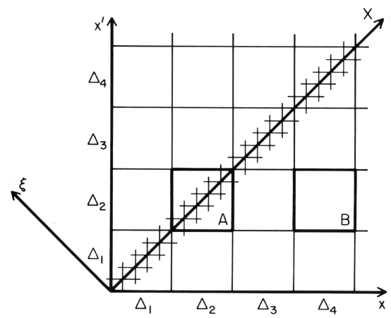
Figure 6: The decoherence of histories coarse-grained by intervals of a distinguished set of configuration space coordinates. The decoherence functional for such sets of histories is defined by the double path integral of (94) over paths $x^{\prime}(t)$ and $x(t)$ that are restricted by the coarse graining. These path integrals may be thought of as the limits of multiple integrals over the values of $x^{\prime}$ and $x$ on a series of discrete time slices of the interval $[0,T]$. A typical slice at a time when the range of integration is constrained by the coarse graining is illustrated. Of course, only one of the distinguished coordinates $x_{a}$ and its corresponding $x^{\prime}_{a}$ can be shown and we have assumed for illustrative purposes that the regions defining the coarse-graining correspond to a set of intervals $\Delta_{\alpha},\alpha=1,2,3,\cdots$ of this coordinate. On each slice where there is a restriction from the coarse graining, the integration over $x^{\prime}$ and $x$ will be restricted to a single box. For the “off-diagonal” elements of the decoherence functional corresponding to distinct histories, that box will be off the diagonal (e.g. B) for some slice. For the diagonal elements, corresponding to the same histories, the box will be on the diagonal (e.g. A) for all slices. If the imaginary part of the influence phase $W[x^{\prime}(\tau),x(\tau)]$ grows as a functional of the difference $\xi(\tau)=x^{\prime}(\tau)-x(\tau)$, as it does in the oscillator models [cf. (82)], then the integrand of the decoherence functional will be negligible except when $x^{\prime}(\tau)$ is close to $x(\tau)$ a regime illustrated by the shaded band about the diagonal in the figure. When the characteristic sizes of the intervals $\Delta_{\alpha}$ are large compared to the width of the band in which the integrand is non-zero the off-diagonal elements of the decoherence functional will be negligible because integrals over those slices where the histories are distinct is negligible (e.g. over box B). That is decoherence of the coarse-grained set of histories. Further, the evaluation of the diagonal elements of the decoherence functional that give the probabilities of the individual histories in decoherent set can be simplified. If the integrations over $x^{\prime}$ and $x$ are transformed to integrations over $\xi=x^{\prime}-x$ and $X=(x^{\prime}+x)/2$ the restrictions on the range of the $\xi$-integration to one diagonal box may be neglected with negligible error to the probability.

Expanding the free action terms in the exponent of (94) is elementary. Assuming the Lagrangian $L_{\rm free}$ consists of a kinetic energy quadratic in the velocities $\dot{x}_{a}$ minus a potential energy independent of the velocities, there is only a contribution from the linear terms in $\xi$ to quadratic order

$$S_{\rm free}[X(\tau)+\xi(\tau)/2]-S_{\rm free}[X(\tau)-\xi(\tau)/2]=\xi^{\dagger}_{0}P_{0}(\dot{X}_{0})+\int\nolimits^{T}_{0}dt\ \xi^{\dagger}(t)\ \left(\frac{\delta S_{\rm free}}{\delta X(t)}\right)+\cdots\,.$$ (95)

Here, $P_{0}(\dot{X}_{0})$ is the canonical momentum, $\partial L_{\rm free}/\partial\dot{X}$, evaluated at the endpoint $t=0$ and expressed in terms of the velocities. $\delta S_{\rm free}/\delta X(t)$ is the usual equation of motion. We are using an obvious matrix notation in which $y^{\dagger}z=\Sigma_{a}y_{a}z_{a}$ and we have used the fact that $\xi_{f}=0$ in (94) to eliminate one surface term.

The general form of the expansion of $W[X(\tau),\xi(\tau)]$ in powers of $\xi(\tau)$ is

$$W[X(\tau),\xi(\tau)]=W[X(\tau),0]+\int\nolimits^{T}_{0}dt\ \xi^{\dagger}(t)\,\left(\frac{\delta W}{\delta\xi(t)}\right)_{\xi(\tau)=0}+{\textstyle{1\over 2}}\int\nolimits^{T}_{0}dt\int\nolimits^{T}_{0}dt^{\prime}\xi^{\dagger}(t)$$

$$\left(\frac{\delta^{2}W}{\delta\xi(t)\delta\xi(t^{\prime})}\right)_{\xi(\tau)=0}\xi(t^{\prime})+\cdots\,.$$ (96)

The coefficients in the expansion can be computed from (92). First,

$$\exp\bigl{(}iW[X(\tau),0]/\hbar\bigr{)}=Sp\left\{U_{T,0}[X(\tau)]\rho_{B}U^{\dagger}_{T,0}[X(\tau)]\right\}=Sp\,\rho_{B}=1\,.$$ (97)

Thus, the leading term in (95) vanishes,

$$W[X(\tau),0]=0\,.$$ (98)

To evaluate the next terms we must consider the derivatives $\delta U_{T,0}[(X(\tau)+\xi(\tau)/2]/\delta\xi(t)$. To do this introduce the definition:

$$F\bigl{(}x(t)\bigr{)}\equiv-\frac{\partial H_{Q}(t)}{\partial x(t)}=\frac{\partial L_{\rm int}\bigl{(}x(t),Q(t)\bigr{)}}{\partial x(t)}\,.$$ (99)

The operator $F(x(t))$ is an operator in the Schrödinger picture in which we have been working. It is a function of $x$ because $L_{\rm{int}}$ is a function of $x$ and becomes a function of $t$ because $x$ is a function $t$. It represents the force on the distinguished subsystem arising from the rest of the closed system.

Carrying out the indicated differentiations of $U$ gives

$$\Bigl{(}\delta U_{T,0}\bigl{[}X(\tau)\pm\xi(\tau)/2\bigr{]}/\delta\xi(t)\Bigr{)}_{\xi(\tau)=0} = \pm(i/2\hbar)U_{T,t}\left[X(\tau)\right]\ F\left(X(t)\right)\,U_{t,0}\left[X(\tau)\right]$$ (100)

$$\equiv \pm(i/2\hbar)\ F\bigl{(}t,X(\tau)\bigr{]}\,.$$

The operator $F(t,X(\tau)]$ is the representative of the Schrödinger operator (99) in a picture something like the Heisenberg picture. However, it is not the usual Heisenberg picture because its connection to the Schrödinger picture involves unitary evolution over future ranges of time to time $T$ as well as past ones. In fact, however, it can be shown GH93 that probabilities are independent of $T$. The operator $F(t,X(\tau)]$ is a function of time but also a functional of the path $X(\tau)$. This dual dependence we have indicated with round and square brackets.

It is then only a short calculation to find for the next coefficient in (96):

$$\bigl{(}\delta W/\delta\xi(t)\bigr{)}_{\xi(\tau)=0}=\bigl{\langle}F\big{(}t,X(\tau)\big{]}\bigr{\rangle}$$ (101)

where the expected value is defined by

$$\langle A\rangle=Sp\left(A\ \rho_{B}\right)\,.$$ (102)

In a similar manner the next coefficient in (96) may be calculated. One finds after slightly more trouble (for more details see GH93 ):

$$\bigl{(}\delta^{2}W/\delta\xi(t)\delta\xi(t^{\prime})\bigr{)}_{\xi(\tau)=0}=(i/2\hbar)\bigl{\langle}\bigl{\{}\Delta F\bigl{(}t,X(\tau)\bigr{]}\,,\ \Delta F\bigl{(}t^{\prime},X(\tau)\bigr{]}\bigr{\}}\bigr{\rangle}$$ (103)

where $\{,\}$ denotes the anticommutator and $\Delta F$ is the operator

$$\Delta F\bigl{(}t,X(t)\bigr{]}=F\bigl{(}t,X(\tau)\bigr{]}-\bigl{\langle}F\bigl{(}t,X(\tau)\bigr{]}\bigr{\rangle}$$ (104)

representing fluctuations in the force $F$ about its mean. We note that $(\delta W/\delta\xi)_{\xi=0}$ is purely real and $(\delta^{2}W/\delta\xi\delta\xi)_{\xi=0}$ is purely imaginary.

With these definitions the Gaussian integral that results from inserting (96) into (94) can be carried out. The result is

$$p(\alpha)\cong\int_{\alpha}\ \delta X\ \bigl{[}{\rm det}\left(K_{I}/4\pi\right)\bigr{]}^{-{\textstyle{1\over 2}}}$$

$$\times\exp\Bigl{[}-\frac{1}{\hbar}\ \int^{T}_{0}\ dt\ \int^{T}_{0}\ dt^{\prime}\ {\cal E}^{\dagger}(t,X(\tau)]\ K^{\rm inv}_{I}(t,t^{\prime};X(\tau)]\ {\cal E}(t^{\prime},X(\tau)]\Bigr{]}w(X_{0},P_{0})\,.$$ (105)

The ingredients of this expression are as follows: ${\cal E}$ is the expression

$${\cal E}(t,X(\tau)]=\frac{\delta S_{\rm free}}{\delta X(t)}+\bigl{\langle}F\bigl{(}t,X(\tau)\bigr{]}\bigr{\rangle}\ .$$ (106)

The kernel $K_{I}$ is

$$K_{I}(t,t^{\prime};X(\tau)]=\hbar^{-1}\bigl{\langle}\bigl{\{}\Delta F\bigl{(}t,X(\tau)\bigr{]},\Delta F(t^{\prime},X(\tau)\bigr{]}\bigr{\}}\bigr{\rangle}\,,$$ (107)

and $K^{\rm inv}_{I}$ is its inverse on the interval $[0,T]$. The function $w$ is the Wigner distribution associated with the initial density matrix $\bar{\rho}$ defined by

$$w\left(X_{0},P_{0}\right)=\int d\xi_{0}\ e^{i(\xi^{\dagger}_{0}P_{0})/\hbar}\bar{\rho}\left(X_{0}+\xi_{0}/2,X_{0}-\xi_{0}/2\right)\,.$$ (108)

For the explicit form of the measure see GH93 .

The expression (105) for the probabilities $p(\alpha)$ has a simple physical interpretation. The kernel $K_{I}(t,t^{\prime})$ is positive because it is the expected value of an anticommutator. The probabilities of histories are therefore peaked about ${\cal E}(t)=0$, that is, about histories which satisfy the equation

$${\cal E}(t)=\frac{\delta S_{\rm free}}{\delta X(t)}+\bigl{\langle}F\bigl{(}t,X(\tau)\bigr{]}\bigr{\rangle}=0\,.$$ (109)

This is the equation of motion of the free action modified by effective forces arising from the interaction of the $x$’s with the rest of the system. In general, these forces will be non-local in time and non-conservative representing such familiar phenomena as friction. As an exercise the reader can show that these forces are causal, that is $\langle F(t,X(\tau)]\rangle$ depends on $X(\tau)$ only for $\tau<t$. The initial positions and momenta are distributed according to the Wigner distribution. The Wigner distribution is not necessarily positive, but the probabilities $p(\alpha)$ are positive by construction apart from small errors that may have been introduced by the approximations mentioned above Hal92 .

Eq. (105) therefore describes the probabilities of a set of histories whose initial conditions are distributed but for which, given an initial condition, the probabilities are peaked about histories satisfying the equation of motion (109). Of course, eq. (105) also shows that there are probabilities for deviations from the equation of motion governed by $K^{\rm inv}_{I}$. These represent noise — both classical and quantum — arising from the interactions of the distinguished system with the rest. Indeed, in this approximation, the probabilities $p(\alpha)$ are identical to those of a classical system obeying a Langevin equation

$${\cal E}(t,X(\tau)]+{\cal L}\bigl{(}t,X(\tau)\bigr{]}=0$$ (110)

with a Gaussian distributed stochastic classical force whose spectrum is fixed by the correlation function

$$\left\langle{\cal L}(t,X(\tau)]{\cal L}(t^{\prime},X(\tau)]\right\rangle_{\rm classical}=\hbar K_{I}\bigl{(}t,t^{\prime};X(\tau)\bigr{]}\,.$$ (111)

If the noise is small, or alternatively, if the parameters of the actions are such that the “width” of the Gaussian distribution of paths is small, then there will be vanishing probabilities for all sufficiently coarse-grained histories $\alpha$ except those correlated in time by the deterministic equation ${\cal E}(t,X(\tau)]=0$. That is classical behavior.

The linear oscillator models of the preceding subsection provide a simple example of the above general analysis. The coefficients $(\delta W/\delta\xi)_{\xi=0}$ and $(\delta^{2}W/\delta\xi\delta\xi)_{\xi=0}$ may be computed directly from (77) and the subsequent expressions for $k_{R}(t,t^{\prime})$ and $k_{I}(t,t^{\prime})$. One finds for the equation of motion

$$-M\ddot{X}-M\omega^{2}X+\int\nolimits^{t}_{0}dt^{\prime}\,k_{R}\left(t,t^{\prime}\right)X\left(t^{\prime}\right)=0$$ (112)

where $k_{R}(t,t^{\prime})$ is given by (78). The spectrum of the noise is simply

$$K_{I}\bigl{(}t,t^{\prime};X(\tau)\bigr{]}=k_{I}\left(t,t^{\prime}\right)$$ (113)

given explicitly by (79). These expressions are even simpler in the high temperature Fokker-Planck limit defined by (85). Then one finds for the equation of motion (away from $t=0$)

$${\cal E}(t,X(\tau)]=-M\ddot{X}(t)-M\omega^{2}X(t)-2M\gamma\dot{X}(t)=0$$ (114)

explicitly exhibiting dissipation. In the same limit the spectrum of noise is

$$K_{I}\bigl{(}t,t^{\prime};X(\tau)\bigr{]}=\frac{8M\gamma kT_{B}}{\hbar}\ \delta\left(t-t^{\prime}\right)\,.$$ (115)

Thus, in this limit, the exponent in the probability formula (94) can be written

$$-\frac{M}{8\gamma kT_{B}}\int\nolimits^{T}_{0}dt\,\left[\ddot{X}+\omega^{2}X+2\gamma\dot{X}\right]^{2}\,.$$ (116)

This expression exhibits explicitly the requirements necessary for classical behavior. Large values of $\gamma T_{B}$ lead to effective decoherence as (85) shows. However, large values of $\gamma T_{B}$ also lead to significant noise (115) and therefore deviations from classical predictability in (116)). To obtain classical predictability, a large coefficient in front of (116) is needed, $M/\gamma T_{B}$ therefore must also be large in the limit that $\gamma T_{B}$ is becoming large. This is a general and physically reasonable result. Stronger coupling to the ignored variables produces more rapid dispersal of phases and more effective decoherence. The same stronger coupling produces greater noise. A high level of inertia is needed to resist this noise and achieve classical predictability.

What this class of models argues for generally is that the classical behavior of a quantum system is an emergent property of its initial condition described by certain decohering sets of alternative coarse-grained histories. Histories of suitable sets are, with high probability, correlated in time by classical deterministic laws with initial data probabilistically distributed according to the system’s initial condition. Coarse graining is required for decoherence and coarse graining beyond that is required to provide the inertia to resist the noise that typical mechanisms of decoherence produce. We may hope to exhibit these conclusions in more general models than those discussed here. In particular in quantum cosmology we hope to exhibit the quasiclassical domain, including the classical behavior of spacetime geometry, as an emergent property of the initial condition of the universe. We shall discuss this further in Section IX but first we must develop a quantum mechanics general enough to deal with spacetime.

IV Generalized Quantum Mechanics

Some of the material in this section has been adapted from the author’s lectures at the 1989 Jerusalem Winter School on Quantum Cosmology and Baby Universes Har91a where the notion of a generalized quantum mechanics was originally introduced.

IV.1 Three Elements

As described in the Introduction, these lectures are concerned with two generalizations of the usual flat spacetime quantum mechanics of measured subsystems that are needed to apply quantum mechanics to cosmology. The first was the generalization to the quantum mechanics of closed systems in which “measurement” does not play a fundamental role. That generalization has been described in the preceding two sections. The remainder of these lectures are concerned with the generalization needed to deal with a quantum theory of gravity in which there is no fixed background spacetime geometry and therefore no fixed notion of time.

We begin, in this section, by abstracting some general principles that define a quantum mechanical theory from the preceding discussion. The resulting framework, called generalized quantum mechanics, provides a general arena for discussing many different generalizations of familiar Hamiltonian quantum mechanics. Among these will be the particular generalization we shall develop for a quantum theory of spacetime.

Roughly speaking, by a generalized quantum mechanics we mean a quantum theory of a closed system that admits a notion of fine- and coarse-grained histories, the decoherence functionals for which are connected by the principle of superposition and for which there is a decoherence condition that determines when coarse-grained histories can be assigned probabilities obeying the sum rules of probability calculus. More precisely, a generalized quantum theory is defined by the following elements:

1. Fine-Grained Histories: The fine-grained histories are the sets of exhaustive, alternative histories of the closed system $\{f\}$ which are the most refined description of its dynamical evolution to which one can contemplate assigning probabilities. Examples are the set of particle paths in non-relativistic quantum mechanics, the set of four-dimensional field configurations in field theory and the set of four-geometries in general relativity as described and qualified in the rest of these lectures. For generality, however, we take $\{f\}$ to be any set here and leave its connection with evolution in spacetime to the specific examples. As the example of non-relativistic quantum mechanics illustrates, there may be many different sets of fine-grained histories.

2. Allowed Coarse Grainings: A set of fine-grained histories may be partitioned into an exhaustive set of exclusive classes $\{c_{\alpha}\}$. That is an operation of coarse graining; each class is a coarse-grained history, and the set of classes is a set of coarse-grained histories. Further partitions of a coarse-grained set are further operations of coarse-graining and yield coarser-grained sets of alternative histories. Conversely, the finer sets are fine grainings of the coarser ones. The process of coarse graining terminates in the trivial case of a set with only a single member — the class $u$ of all fine-grained histories — which we assume to be a common coarse graining for all fine-grained sets.

   The sets of exclusive histories arrived at by operations of coarse graining exhaust the alternatives of the closed system to which generalized quantum mechanics potentially assigns probabilities. The set of all sets of histories is partial ordered by the operations of coarse and fine graining because two given sets need not be either fine or coarse grainings of each other. For convenience we may regard the fine-grained sets as coarse-grained sets with a trivial coarse graining. The set of coarse-grained sets of histories is then a semi-lattice.

3. Decoherence Functional: Interference between the members of a coarse-grained set of histories is measured by the decoherence functional. The decoherence functional is a complex-valued functional, $D(\alpha^{\prime},\alpha)$, defined for each pair of histories in a coarse-grained set $\{\alpha\}$. The decoherence functional for each set of alternative coarse-grained histories must satisfy the following conditions:

   1. Hermiticity:

      $$D(\alpha^{\prime},\alpha)=D^{*}(\alpha,\alpha^{\prime})\,,$$ (117a)

   2. Positivity:

      $$D(\alpha^{\prime},\alpha)\geq 0\,,$$ (117b)

   3. Normalization:

      $$\sum\limits_{\alpha^{\prime},\alpha}D(\alpha^{\prime},\alpha)=1\,.$$ (117c)

      In addition, and most importantly, the decoherence functional for different coarse-grained sets must be related by the principle of superposition:

   4. The principle of superposition:

      $$D(\bar{\alpha}^{\prime},\bar{\alpha})=\sum\limits_{\alpha^{\prime}\epsilon\bar{\alpha}^{\prime}}\sum\limits_{\alpha\epsilon\bar{\alpha}}D(\alpha^{\prime},\alpha)\,.$$ (117d)

The superposition principle means that once the decoherence functional is defined for any fine-grained set of histories, $\{f\}$, the decoherence functional for any coarse-graining of it may be determined by (117d). If there is a unique most fine-grained set, as in a sum-over-histories formulation of quantum mechanics, then the specification of a $D(f^{\prime},f)$ consistent with (117a) – (117c) specifies all other decoherence functionals. If there is more than one most fine-grained set $\{f\}$, then the decoherence functional must be specified consistently so that if a set of alternative histories is a coarse-graining of two different fine-grained sets of the same decoherence results from (117d) applied to the different fine-grained sets.

The specification of a generalized quantum mechanics is completed by giving a decoherence condition that specifies which sets of alternative coarse-grained histories are assigned probabilities in the theory. Such sets of histories are said to decohere. The probabilities of the individual histories in a decoherent set are the “diagonal” elements of the decoherence functional

$$p(\alpha)=D(\alpha,\alpha)\,.$$ (118)

These must satisfy the general rules of probability theory (e.g. as in Fel57 ). They must be real numbers between zero and one defined on the sample space supplied by a set of alternative coarse-grained histories. The probabilities must be additive on disjoint sets of the sample space which in the present instance means

$$p(\bar{\alpha})=\sum\limits_{\alpha\epsilon\bar{\alpha}}p(\alpha)\,,$$ (119)

for any coarse-graining $\{c_{\bar{\alpha}}\}$ of $\{c_{\alpha}\}$, to the approximation with which the probabilities are used. The probability of the empty set, $\phi$, must be zero and the probability of the whole set, $u$, must be one.

The simplest decoherence condition is the requirement that the “off-diagonal” elements of the decoherence functional be sufficiently small

$$D\left(\alpha^{\prime},\alpha\right)\approx 0\ ,\quad\alpha^{\prime}\not=\alpha\,.$$ (120)

This was the sufficient condition for the probability sum rules used in Sections II and III and the decoherence condition we shall assume in the rest of this paper. As a consequence, the conditions (117a)–(117d) of (117) the numbers defined by (118) obey the rules of probability theory for sets of histories obeying the decoherence condition (120). They are real and positive because of the hermiticity and positivity conditions. They sum to unity by the normalization condition and they obey the sum rules (119) because of the principle of superposition, viz.

$$p(\bar{\alpha})=D(\bar{\alpha},\bar{\alpha})=\sum\limits_{\alpha^{\prime}\epsilon\bar{\alpha}}\,\sum\limits_{\alpha\epsilon\bar{\alpha}}\,D(\alpha^{\prime},\alpha)\approx\sum\limits_{\alpha\epsilon\bar{\alpha}}\,D(\alpha,\alpha)=\sum\limits_{\alpha\epsilon\bar{\alpha}}\,p(\alpha)\,.$$ (121)

Decoherence conditions both stronger and weaker than (120) have been investigated. (See GH90b and GH93 for discussion.) If arbitrary unions of coarse-grained histories into new, mutually exclusive classes are allowed operations of coarse graining, then it is not difficult to see that the necessary as well as sufficient condition for the probability sum rules (119) to be satisfied is [cf. (46)]

$$Re\,D\left(\alpha^{\prime},\alpha\right)\approx 0\ ,\quad\alpha^{\prime}\not=\alpha\,.$$ (122)

Conditions (122) and (120) are called the weak and medium decoherence conditions, respectively. An even weaker condition was used by Griffiths Gri84 and Omnès Omnsum in their original investigations, and conditions stronger than medium decoherence have been investigated in the efforts to precisely characterize quasiclassical domains GH93 .

A choice between weak, medium, or other forms of the decoherence condition is not really needed for the rest of the discussion of generalizations of quantum mechanics that are free from the problem of time since we shall not carry out explicit calculations of the decoherence of specific sets of histories. All that is necessary is that the condition be expressed in terms of the decoherence functional. For simplicity, the reader can keep in mind the medium decoherence condition (120). Realistic mechanisms of decoherence, such as those illustrated in Section III, lead to medium decoherence.

These three elements — fine-grained histories, coarse-graining, and a decoherence functional together with a decoherence condition — capture the essential features of quantum mechanical prediction. In the following we shall see that Hamiltonian quantum mechanics is one way of specifying these elements but not the only way. Alternative specifications lead to generalizations of Hamiltonian quantum mechanics. In the remainder of this section we discuss some familiar formulations of quantum mechanics from the generalized quantum mechanics point of view.

IV.2 Hamiltonian Quantum Mechanics as a Generalized Quantum Mechanics

First, we consider Hamiltonian quantum mechanics as a generalized quantum mechanics. In Hamiltonian quantum mechanics sets of histories are represented by chains of projections onto exhaustive sets of orthogonal subspaces of a Hilbert space. The fine-grained histories, coarse graining, and decoherence functional are specified as follows:

1. Fine-Grained Histories: These correspond to the possible sequences of sets of projections onto a complete set of states, one set at every time. There are thus many different sets of fine-grained histories corresponding to the various possible complete sets of states at each and every time. The many possible fine-grained starting points in Hamiltonian quantum mechanics are a reflection of the democracy of transformation theory. No one basis is distinguished from any other.

2. Allowed Coarse Grainings: For definiteness, we take the allowed sets of coarse-grained histories of Hamiltonian quantum mechanics to consist of sequences of independent alternatives at definite moments of time so that every history can be represented as a chain of projections as in (14). A set of such histories is a coarse graining of a finer set if each projection in the coarser grained set is a sum of projections in the finer grained set. The projections constructed as sums define a partition of the histories in the finer grained set.

   By way of example, consider the quantum mechanics of a particle. A very fine-grained set of histories can be specified by very small position intervals at a great many times thus approximately specifying the particle’s path in configuration space. An example of coarse graining of these consists of projections onto an exhaustive set of ranges of position at, say, three different times defining a partition of the configuration space paths into those that pass through the various possible combinations of ranges at the different times.

   Given the discussion in Section III.1.1 on the importance of branch dependence, it may seem arbitrary to limit the coarse-grained sets of histories of Hamiltonian quantum mechanics to be always represented by chains of projections and not sums of chains of projections. We do so to ensure, as discussed in Section III.1.3, that evolution in Hamiltonian quantum mechanics can be formulated in the familiar terms of a state vector that evolves unitarily in between alternatives and is reduced at them. Incorporating branch dependent histories represented by sums of chains of projections we consider as a generalization of Hamiltonian quantum mechanics.

   

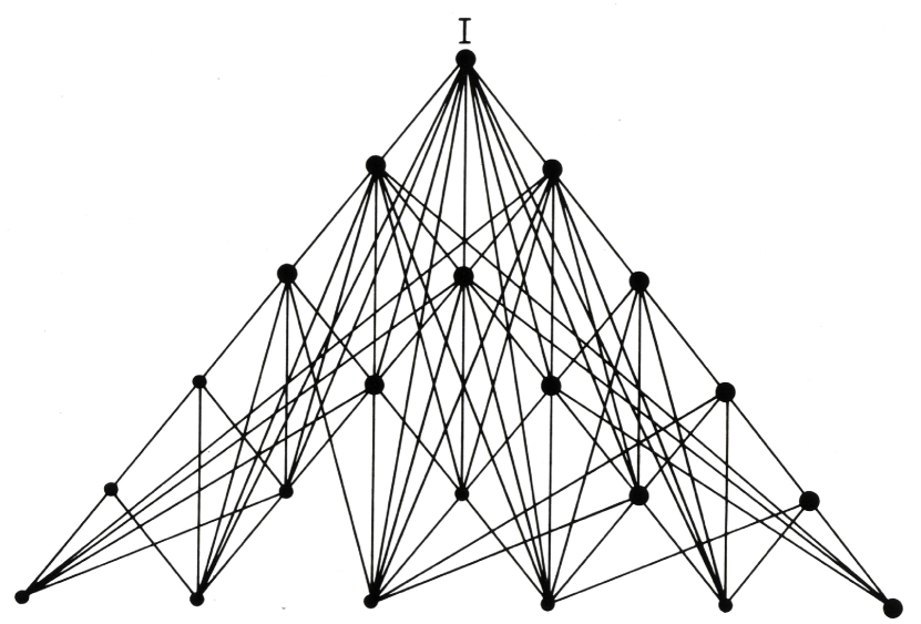
   Figure 7: The schematic structure of the space of sets of possible histories in Hamiltonian quantum mechanics. Each dot in this diagram represents an exhaustive set of alternative histories for the universe. (This is not a picture of the branches defined by a given set!)  Such sets correspond in the Heisenberg picture to time sequences ($P^{1}_{\alpha_{1}}(t_{1}),\ P^{2}_{\alpha_{2}}(t_{2}),\ \cdots\ P^{n}_{\alpha_{n}}(t_{n}))$ of sets of projection operators, such that at each time $t_{k}$ the alternatives $\alpha_{k}$ are an orthogonal and exhaustive set of possibilities for the universe. At the bottom of the diagram are the completely fine-grained sets of histories each arising from taking projections onto eigenstates of a complete set of observables for the universe at every time.
   The dots above the bottom row are coarse-grained sets of alternative histories. If two dots are connected by a path, the one above is a coarse graining of the one below — that is, the projections in the set above are sums of those in the set below. A line, therefore, corresponds to an operation of coarse graining. At the very top is the degenerate case in which complete sums are taken at every time, yielding no projections at all other than the unit operator! The space of sets of alternative histories is thus partially ordered by the operation of coarse graining.
   The heavy dots denote the decoherent sets of alternative histories. Coarse grainings of decoherent sets remain decoherent.

3. Decoherence Functional: For Hamiltonian quantum mechanics this is (40). In the present notation $\alpha$ stands for the history corresponding to a particular chain of projections $C_{\alpha}$. Thus,

   $$D(\alpha^{\prime},\alpha)=Tr\,\bigl{[}C_{\alpha^{\prime}}\rho C^{\dagger}_{\alpha}\bigr{]}=Tr\bigl{[}P^{n}_{\alpha^{\prime}_{n}}(t_{n})\cdots P^{1}_{\alpha^{\prime}_{1}}(t_{1})\rho P^{1}_{\alpha_{1}}(t_{1})\cdots P^{n}_{\alpha_{n}}(t_{n})\bigr{]}$$ (123)

   which is easily seen to satisfy properties (117a)–(117d) above.

   The structure of sets of alternative coarse-grained histories of Hamiltonian quantum mechanics is shown schematically in Fig. 7. The sets of coarse-grained histories form a partially ordered set defining a semi-lattice. For any pair of sets of histories, the least coarse grained set of which they are both fine grainings can be defined. However, there is not, in general, a unique most fine-grained set of which two sets are a coarse graining.

IV.3 Sum-Over-Histories Quantum Mechanics for Theories with a Time.

The fine-grained histories, coarse graining, and decoherence functional of a sum-over-histories quantum mechanics of a theory with a well defined physical time are specified as follows:

1. Fine-Grained Histories: The fine-grained histories are the possible paths in a configuration space of generalized coordinates $\{q^{i}\}$ expressed as single-valued functions of the physical time. Only one configuration is possible at each instant. Sum-over-histories quantum mechanics, therefore, starts from a unique fine-grained set of alternative histories of the universe in contrast to Hamiltonian quantum mechanics that starts from many.

2. Allowed Coarse Grainings: There are many ways of partitioning the fine-grained paths into exhaustive and exclusive classes, $\{c_{\alpha}\}$. However, the existence of a physical time allows an especially natural coarse graining because paths cross a constant time surface in the extended configuration space $(t,q^{i})$ once and only once. Specifying an exhaustive set of regions $\{\Delta_{\alpha}\}$ of the $q^{i}$ at one time, therefore, partitions the paths into the class of those that pass through $\Delta_{1}$ at that time, the class of those that pass through $\Delta_{2}$ at that time, etc. More generally, different exhaustive sets of regions $\{\Delta^{k}_{\alpha_{k}}\}$ at times $\{t_{k}\}$, $k=1,\cdots,n$ similarly define a partition of the fine-grained histories into exhaustive and exclusive classes. More general partitions of the configuration space paths corresponding to alternatives that are not at definite moments of time will be described in Section V.

3. Decoherence Functional: The decoherence functional for sum-over-histories quantum mechanics for theories with a well-defined time is

   $$D(\alpha^{\prime},\alpha)=\int\nolimits_{\alpha}\delta q^{\prime}\int\nolimits_{\alpha}\delta q\delta(q^{\prime}_{f}-q_{f})\ \exp\biggl{\{}i\left(S[q^{\prime}(\tau)]-S[q(\tau)]\right)/\hbar\biggr{\}}\rho(q^{\prime}_{0},q_{0})\,.$$ (124)

   Here, we consider an interval of time from an initial instant $t=0$ to some final time $t=T$. The first integral is over paths $q(t)$ that begin at $q_{0}$, end at $q_{f}$, and lie in the class $c_{\alpha}$. The integral includes an integration over $q_{0}$ and $q_{f}$. The second integral over paths $q^{\prime}(t)$ is similarly defined. If $\rho(q^{\prime},q)$ is a density matrix, then it is easy to verify that $D$ defined by (124) satisfies conditions (i)–(iv) of (117). When the coarse graining is defined by sets of configuration space regions $\{\Delta^{k}_{\alpha_{k}}\}$ as discussed above, then (124) coincides with the sum-over-histories decoherence functional previously introduced in (59). However, more general partitions are possible.

The structure of the collection of sets of coarse-grained histories in sum-over-histories quantum mechanics is illustrated in Fig. 8. Because there is a unique fine grained set of histories, many fewer coarse grainings are possible in a sum-over-histories formulation than in a Hamiltonian one, and the space of sets of coarse-grained histories is a lattice rather than a semi-lattice.

IV.4 Differences and Equivalences between Hamiltonian and Sum-Over-Histories
Quantum Mechanics for Theories with a Time

From the perspective of generalized quantum theory, the sum-over-histories quantum mechanics of Section IV.3 is different from the Hamiltonian quantum mechanics of Section IV.2. Even when the action of the former gives rise to the Hamiltonian of the latter, the two formulations differ in their notions of fine-grained histories, coarse graining and in the resulting space of coarse-grained sets of histories as Figs 7 and 8 clearly show. Yet, as we demonstrated in Section III.1.4, the sum-over-histories formulation and the Hamiltonian formulation are equivalent for those particular coarse grainings in which the histories are partitioned according to exhaustive sets of configuration space regions, $\{\Delta^{k}_{\alpha_{k}}\}$, at various times $t_{k}$. More precisely the sum-over-histories expression for the decoherence functional, (124), is equal to the Hamiltonian expression, (IV.2.1), when the latter is evaluated with projections onto the ranges of coordinates that occur in the former. Crucial to this equivalence, however, is the existence of a well-defined physical time in which the paths are single-valued which permitted the factorization of the path integral in (56) that led to the identity (54) which connected the two formulations.

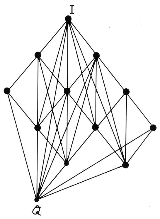
Figure 8: The schematic structure of the space of sets of histories in sum-over-histories quantum mechanics. The completely fine-grained histories arise from a single complete set of observables, say the set ${\cal Q}$ of field variables $q^{i}$ at each point in space and every time.

To see this more clearly let us sketch the derivation of a Hamiltonian formulation from a sum-over-histories one — the inverse of the construction described in Section III.1.4. For simplicity consider a partition of the paths by an exhaustive set of configuration space regions $\{\Delta_{\alpha}\}$ at a single time intermediate time, $t$. We could note that the decoherence functional (124) could be rewritten in the form (56) where the quantities $\langle q_{f}T|C_{\alpha}|q_{0}0\rangle$ are now defined by

$$\bigl{\langle}q_{f}T|C_{\alpha}|q_{0}0\bigr{\rangle}=\int\nolimits_{[q_{0}\alpha q_{f}]}\delta q\,e^{iS[q(\tau)]/\hbar}\,.$$ (125)

If the paths $q(\tau)$ are single valued in time, the path-integral may be factored using the identity (54) (cf. Fig. 7) into an integral over paths before $t$, an integral over paths after $t$, and an integral over the region $\Delta_{\alpha}$ at $t$. The integrals over paths before $t$ may be taken to define a wave function on the surface $t=t_{k}$, viz.

$$\psi_{(q_{0}0)}(q,t)=\int_{[q_{0}\,q_{k}]}\delta q\,e^{iS[q(\tau)]/\hbar}\,.$$ (126)

The integral over the paths after $t$ may be taken to define the complex conjugate of a wave function $\psi_{(q_{f}T)}(q\,t)$. The matrix elements (125) are then given by

$$\bigl{\langle}q_{f}T\left|C_{\alpha}\right|q_{0}0\bigr{\rangle}=\int\nolimits_{\Delta_{\alpha}}dq\psi^{*}_{(q_{f}T)}(q,t)\psi_{(q_{0}0)}(q,t)$$ (127)

thus defining an inner product on wave functions. If we vary the time $t$ it is an elementary consequence of the definition (126) that the wave functions satisfy the Schrödinger equation and the inner product is preserved FH65 . In this way we would be led to a Hamiltonian quantum mechanics of states on spacelike surfaces evolving unitarily and by reduction of the wave packet. Two things were crucial to this derivation. First, the existence of a set of surfaces in the extended configuration space $(t,q^{i})$ which the paths crossed once and only once thus defining a notion of time. Second, a coarse graining that restricted the paths only on constant time surfaces. In the subsequent sections we shall discuss more general coarse grainings and cases where there are no such surfaces and no associated time. An equivalent Hamiltonian formulation cannot then be expected.

Thus, despite their equivalence on certain coarse-grained sets of alternative histories, Hamiltonian quantum mechanics and sum-over-histories quantum mechanics are different because their underlying sets of fine-grained histories are different. Indeed, as we have presented them, the fine-grained histories are defined in different spaces in the two cases — a space of paths in the sum-over-histories formulation and the space of chains of projections on ${\cal H}$ in the Hamiltonian formulation. Are the more limited coarse grainings of sum-over-histories quantum mechanics adequate for physics? They are if all testable statements can be reduced to statements about configuration space variables — positions, fields of integer and half-integer spin, etc. Certainly this would seem sufficient to describe the coarse graining associated with any classical domain.

In the following we shall see that the sum-over-histories formulation of quantum mechanics provides an accessible route for investigating generalizations of Hamiltonian quantum mechanics that covariantly resolve the problem of time in quantum gravity. The route is accessible because the main objective of these generalizations will be to cast quantum mechanics into fully four-dimensional form that does not require a preferred time. In sum-over-histories quantum mechanics the fine-grained histories are spacetime paths and dynamics in summarized by an action functional on these paths. One is thus well along the way to the desired objective and the conceptual clarity afforded by the sum-over-histories formulation is of considerable help with the rest. Because of this conceptual clarity, because a sum-over-histories formulation may be general enough for all realistic applications of quantum mechanics, and for reasons of simplicity and economy we shall focus on sum-over-histories generalized quantum mechanics in what follows.

This focus should not be interpreted to mean that we eschew operator methods in quantum mechanics. As we shall describe in Section V, continuous operator products can be used to rigorously explore the limits that define certain path integrals. More importantly, such products can be used to define generalizations of at least some of the sum-over-histories frameworks that we explore which incorporate the richer variety of coarse grainings of transformation theory. Operators and path integrals are therefore not in conflict and often complementary. It is for clarity and simplicity that we focus on sum-over-histories formulations in these lectures.

IV.5 Classical Physics and the Classical Limit of Quantum Mechanics.

Classical physics may be regarded as a trivial generalized quantum mechanics. The basic elements are:

1. Fine-grained histories: The fine-grained histories are paths in phase space, $(p_{i}(t),\ q^{i}(t))$, parametrized by the physical time.

2. Allowed Coarse grainings: The most familiar type of coarse graining is specified by cells in phase space at discrete sequences of time. The paths are partitioned into classes defined by which cells they pass through.

3. Decoherence Functional: From the perspective of quantum theory, the distinctive features of classical physics are that the fine-grained histories are exactly decoherent and exactly correlated in time according to classical dynamical laws. A decoherence functional that captures these features may be constructed as follows:

   Let $z^{i}=(p_{i},\ q^{i})$ serve as a compact notation for a point in phase space. $z^{i}(t)$ is a phase space path. Let $z^{i}_{cl}(t;z^{i}_{0})$ denote the path that is the classical evolution of the initial condition $z^{i}_{0}$ at time $t_{0}$. The path $z^{i}_{cl}(t)=(p^{cl}_{i}(t),\ q^{i}_{cl}(t))$ satisfies the classical equations of motion:

   $$\dot{p}^{cl}_{i}=-\frac{\partial H}{\partial q^{i}_{cl}}\quad,\quad\dot{q}^{i}_{cl}=\frac{\partial H}{\partial p^{cl}_{i}}\,,$$ (128)

   where $H$ is the classical Hamiltonian, with the initial condition $z^{i}(t_{0};z^{i}_{0})=z^{i}_{0}$. Define a classical decoherence functional, $D_{cl}$, on pairs of fine-grained histories as

   $$D_{cl}[z^{\prime i}(t),\ z^{i}(t)]\equiv\delta[z^{\prime i}(t)-z^{i}(t)]\int d\mu(z^{i}_{0})\delta[z^{i}(t)-z^{i}_{cl}(t;z_{0})]f(z^{i}_{0})\,.$$ (129)

   Here $\delta[\cdot]$ denotes a functional $\delta$-function on the space of phase space paths, and $d\mu(z^{i})$ is the usual Liouville measure, $\Pi_{i}[dp_{i}\,dq^{i}/(2\pi\hbar)]$. The function $f(z^{i}_{0})$ is a real, positive, normalized distribution function on phase space which gives the initial condition of the closed classical system. The first $\delta$-function in (129) enforces the exact decoherence of classical histories; the second guarantees correlation in time according to classical laws.

   A coarse graining of the set of alternative fine-grained histories may be defined by giving exhaustive partitions of phase space into regions $\{R^{k}_{\alpha_{k}}\}$ at a sequence of times $t_{k}$, $k=1$, $\cdots,n$. Here, $\alpha$ labels the region and $k$ the partition. The decoherence functional for the corresponding set of coarse-grained alternative classical histories is

   $$D_{cl}\left(\alpha^{\prime},\alpha\right)=\int\nolimits_{\alpha^{\prime}}\delta z^{\prime}\int\nolimits_{\alpha}\delta zD_{cl}[z^{\prime i}(t),z^{i}(t)]\,,$$ (130)

   where the integral is over pairs of phase space paths restricted by the appropriate regions and the integrand is (129). It is then also easy to see that (130) and (129) satisfy the conditions (117a) – (117d) of Section IV.1 for decoherence functionals. For all coarse grainings one has

   $$D_{cl}\left(\alpha^{\prime},\alpha\right)=\delta_{\alpha^{\prime}_{1}\alpha_{1}}\cdots\delta_{\alpha^{\prime}_{n}\alpha_{n}}\ p_{cl}(\alpha_{1},\cdots,\alpha_{n})\,,$$ (131)

   where $p_{cl}(\alpha_{1},\cdots,\alpha_{n})$ is the classical probability to find the system in the sequence of phase space regions $\alpha_{1},\cdots,\alpha_{n}$ given that it is initially distributed according to $f(z^{i}_{0})$.

   It is not just as an academic exercise that we reformulate classical mechanics as a trivial generalized quantum mechanics. This reformulation enables us to give a more precise statement of the classical limit of quantum mechanics. In certain situations the decoherence functional of a quantum mechanics may be well approximated by a classical decoherence functional of the form (130). For example, in Hamiltonian quantum mechanics it may happen that for some coarse grained set of alternative histories $\{\alpha\}$

   $$D\left(\alpha^{\prime},\alpha\right)=Tr[C_{\alpha^{\prime}}\rho\,C^{\dagger}_{\alpha}]\cong D_{cl}\left(\alpha^{\prime},\alpha\right)\,,$$ (132)

   for some corresponding coarse graining of phase space $\{R^{k}_{\alpha_{k}}\}$ and distribution function $f$. One has then exhibited the classical limit of quantum mechanics.

   Some coarse graining is needed for a relation like (132) to hold because otherwise the histories, $\{c_{\alpha}\}$, would not decohere. Moreover, a relation like (132) cannot be expected to hold for every coarse graining. Roughly, we expect that the projections $\{P^{k}_{\alpha_{k}}\}$ must correspond to phase space regions, for example, by projecting onto sufficiently crude intervals of configuration space and momentum space or onto coherent states corresponding to regions of phase space. (See, e.g. Hep74 , Omn89 , and Cav94 for more on this.) Moreover, for a fixed coarse graining, a relation like (132) cannot hold for every initial condition $\rho$. Only for particular coarse grainings and particular $\rho$ do we recover the classical limit of a quantum mechanics in the sense of (132)

IV.6 Generalizations of Hamiltonian Quantum Mechanics

As the preceding example of classical physics illustrates, there are many examples of generalized quantum mechanics that do not coincide with Hamiltonian quantum mechanics. The requirements for a generalized quantum mechanics are weak. Fine-grained histories, a notion of coarse graining, and a decoherence functional and decoherence condition are all that is needed. There are probably many such constructions. It is thus important to search for further physical principles with which to winnow these possibilities. In this search there is also the scope to investigate whether the familiar Hamiltonian formulation of quantum mechanics might not itself be an approximation to some more general theoretical framework appropriate only for certain coarse grainings and particular initial conditions of the universe. If $D$ were the decoherence functional of the generalization then

$$D(\alpha^{\prime},\alpha)\cong Tr\bigl{[}C_{\alpha^{\prime}}\,\rho\,C^{\dagger}_{\alpha}\bigr{]}$$ (133)

only for certain $\{c_{\alpha}\}$’s and corresponding $C$’s and for a limited class of $\rho$’s. Thus, in cosmology it is possible to investigate which features of Hamiltonian quantum mechanics are fundamental and which are “excess baggage” that only appear to be fundamental because of our position late in a particular universe able to employ only limited coarse grainings. In the next sections we shall argue that one such feature is the preferred time of Hamiltonian quantum mechanics.

IV.7 A Time-Neutral Formulation of Quantum Mechanics

The Hamiltonian quantum mechanics based on the decoherence functional (123) is not time neutral. The future is treated differently from the past so that the theory incorporates a fundamental, quantum-mechanical arrow of time. As a first serious example of a generalized quantum mechanics we shall describe a time-neutral generalization of quantum mechanics that does not single out an arrow of time.

The quantum-mechanical arrow incorporated into the decoherence functional (123) does not arise because of the time ordering of the chains of projection operators. Field theory is invariant under $CPT$ and the ordering can be reversed by a $CPT$ transformation of the projection operators and density matrix. To see this, let $\Theta$ denote the antiunitary $CPT$ transformation and, for simplicity, consider alternatives $\{P^{k}_{\alpha_{k}}(t_{k})\}$ such that their $CPT$ transforms, $\{\widetilde{P}^{k}_{\alpha_{k}}(-t_{k})\}$, are given by

$$\widetilde{P}^{k}_{\alpha_{k}}(-t_{k})=\Theta^{-1}P^{k}_{\alpha_{k}}(t_{k})\Theta\,.$$ (134)

Since the Hamiltonian is invariant under $CPT$ these $CPT$ transforms continue to be related to each other at different times by (35). Under $\Theta$, a sequence of alternatives at times $t_{1}<t_{2}<\cdots<t_{n}$ that is represented by the chain

$$C_{\alpha}=P^{n}_{\alpha_{n}}(t_{n})\cdots P^{1}_{\alpha_{1}}(t_{1})$$ (135)

is transformed into a sequence of $CPT$ transformed alternatives with the reversed time ordering $-t_{n}<\cdots<-t_{2}<-t_{1}$ represented by the chain

$$\widetilde{C}^{\rm rev}_{\alpha}\equiv\Theta^{-1}C_{\alpha}\Theta=\widetilde{P}^{n}_{\alpha_{n}}(-t_{n})\cdots\widetilde{P}^{1}_{\alpha_{1}}(-t_{1})$$ (136)

and similarly for alternatives represented by sums of chains. If the density matrix is also transformed

$$\tilde{\rho}=\Theta^{-1}\rho\Theta\,,$$ (137)

then the decoherence functional is complex conjugated

$$\widetilde{D}^{\rm rev}\left(\alpha^{\prime},\alpha\right)=Tr\bigl{[}\widetilde{C}^{\rm rev}_{\alpha^{\prime}}\tilde{\rho}\,\widetilde{C}^{{\rm rev}\dagger}_{\alpha}\bigr{]}=Tr[\Theta^{-1}C_{\alpha^{\prime}}\Theta\Theta^{-1}\rho\Theta\Theta^{-1}C^{\dagger}_{\alpha}\Theta]$$

$$=Tr\bigl{[}\Theta^{-1}C_{\alpha^{\prime}}\rho\,C^{\dagger}_{\alpha}\Theta\bigr{]}=D^{*}\left(\alpha^{\prime},\alpha\right)\,.$$ (138)

In the last step the antiunitarity of $\Theta$ which implies $(\psi,\Theta^{-1}\phi)=(\Theta\psi,\phi)^{*}$ has been used. Decoherent sets of histories are thus transformed into decoherent sets of histories, their probabilities are unchanged, but the time ordering has been reversed. Either time ordering may therefore be used in formulating quantum mechanics. It is by convention that we use the ordering in which the projection with the earliest time is closest to the density matrix in (123), that is, the ordering in which the density matrix is in the past.

The difference between the future and the past in the usual formulation of quantum mechanics arises therefore, not from the time-ordering of the projections representing histories, but rather because the ends of the histories are treated asymmetrically in (123). At one end of the chains of projections (conventionally the past) there is a density matrix. At the other end (conventionally the future) there is the trace. Whatever conventions are used for time ordering there is thus an asymmetry between future and past exhibited by (123). That asymmetry is the arrow of time in quantum mechanics.

The observed universe exhibits general time asymmetries. These include

• The thermodynamic arrow of time — the fact that approximately isolated systems are now almost all evolving towards equilibrium in the same direction of time.

• The psychological arrow of time — we remember the past, we predict the future.

• The arrow of time of retarded electromagnetic radiation.

• The arrow of time supplied by the $CP$ non-invariance of the weak interactions and the $CPT$ invariance of field theory.

• The arrow of time of the approximately uniform expansion of the universe.

• The arrow of time supplied by the growth of inhomogeneity in the expanding universe.

All of the time asymmetries on this list could arise from time-symmetric dynamical laws solved with time-asymmetric boundary conditions. The thermodynamic arrow of time, for example, is implied by an initial condition in which the progenitors of today’s approximately isolated systems were all far from equilibrium at an initial time. The $CP$ arrow of time could arise as a spontaneously broken symmetry of the Hamiltonian Lee88 . The approximate uniform expansion of the universe and the growth of inhomogeneity follow from an initial “big bang” of sufficient spatial homogeneity and isotropy, given the attractive nature of gravity. Characteristically such arrows of time can be reversed temporarily, locally, in isolated subsystems, although typically at an expense so great that the experiment can be carried out only in our imaginations. If we could, in the classical example of Loschmidt Los76 , reverse the momenta of all particles and fields of an isolated subsystem, it would “run backwards” with thermodynamic and electromagnetic arrows of time reversed.

In contrast to the time asymmetries mentioned above, in the quantum mechanics of closed systems a quantum mechanical arrow of time would be fundamental and not reversible. That is not inconsistent with observation because, as we have just described, all of the observed arrows of time could be explained by special properties of the initial $\rho$ in the usual formulation of quantum mechanics. All such arrows of time would therefore coincide with the fundamental quantum mechanical arrow of time. However, as we shall now show, all the arrows of time, including the quantum mechanical one, can be put on the same footing in a time-neutral generalization of quantum mechanics.

Nearly thirty years ago, Aharonov, Bergmann, and Lebovitz ABL64 showed how to cast the quantum mechanics of measured subsystems into time-neutral form by considering final conditions as well as initial ones. The same type of framework for the quantum mechanics of closed systems has been discussed by Griffiths Gri84 and by Gell-Mann and the author Har91a and GH93b as an example of generalized quantum mechanics. The fine-grained histories and coarse grainings of this generalized quantum mechanics are the same as for usual Hamiltonian quantum mechanics as described in Section IV.2. Only the decoherence functional differs by employing both initial and final density matrices. It is

$$D\left(\alpha^{\prime},\alpha\right)={\cal N}\,Tr\left[\rho_{f}C_{\alpha^{\prime}}\rho_{i}C^{\dagger}_{\alpha}\right]$$ (139a)

where

$${\cal N}^{-1}=Tr\left(\rho_{f}\rho_{i}\right)\,.$$ (139b)

Here, $\rho_{i}$ and $\rho_{f}$ are Hermitian, positive operators that we may conventionally call Heisenberg operators representing the initial and final conditions. They need not be normalized as density matrices with $Tr(\rho)=1$ because (139) is invariant under changes of normalization. It is easy to verify that (139) satisfies the four requirements (117). There is a similar generalization for sum-over-histories quantum mechanics found by replacing $\delta(q^{\prime}_{f}-q_{f})$ in (124) by a final density matrix in configuration space $\rho_{f}(q^{\prime}_{f},q_{f})$ and multiplying by the same normalizing factor.

The decoherence functional (139) is time-neutral. There is a density matrix at both ends of each history. Initial and final conditions may be interchanged by making use of the cyclic property of the trace. Therefore, the quantum mechanics of closed systems based on (139) does not have a fundamental arrow of time. Different quantum-mechanical theories of cosmology are specified by different choices for the initial and final conditions $\rho_{i}$ and $\rho_{f}$. For those cases with $\rho_{f}\propto I$, where $I$ is the unit matrix, this formulation reduces to the usual one because then (139) coincides with (123).

Lost in this generalization is a built-in notion of causality in quantum mechanics. Lost also, when $\rho_{f}$ is not proportional to $I$, is any notion of a unitarily evolving “state of the system at a moment of time”. We cannot construct an effective density matrix at one time analogous to (51) from which alone probabilities for both future and past can be calculated. What is gained is a quantum mechanics without a fundamental arrow of time in which all time asymmetries could arise in particular cosmologies because of differences between $\rho_{i}$ and $\rho_{f}$ or at particular epochs from their being near the beginning or the end. That generalized quantum mechanics embraces a richer variety of possible universes, allowing for the possibility of violations of causality and advanced as well as retarded effects. These, therefore, become testable features of the universe rather than axioms of the fundamental quantum framework.

From the perspective of this generalized quantum mechanics, the task of quantum cosmology is to find a theory of both the initial and final conditions that is theoretically compelling and fits our existing data as well as possible. A final condition of indifference $\rho_{f}=I$ and a special initial condition $\rho_{i}$ would seem to fit well and give rise to the observed arrows of time including the quantum mechanical one. More general conditions can be considered. In the following we shall adopt this more general and symmetric approach to quantum cosmology.

V The Spacetime Approachto Non-Relativistic Quantum
Mechanics

V.1 A Generalized Sum-Over-Histories Quantum Mechanics for Non-Relativistic
Systems

As mentioned in the Introduction, an objective of these lectures is to generalize usual quantum mechanics to put it in fully spacetime form so that it can provide a covariant quantum theory of spacetime. We shall employ the strategy of first developing these ideas in a series of model problems which illuminate various aspects of the general relativistic case.

The most elementary model is non-relativistic particle quantum mechanics which we consider in this section. We discussed non-relativistic, sum-over-histories quantum mechanics as a generalized quantum mechanics in Section IV.3. However, we did not exhibit the theory in fully spacetime form. The sum-over-histories formulation did cast quantum dynamics into spacetime form involving spacetime histories directly and summarized by an action that is a functional of particle paths. However, our discussion of the coarse grainings to which the theory potentially assigns probabilities was limited to those defined by alternative ranges of coordinates at definite moments of time. Were these the most general alternatives for which a quantum theory could predict probabilities it would inevitably involve a preferred notion of time. More general spacetime coarse grainings are easy to imagine. For instance, we may partition the paths by their behavior with respect to a spacetime region $R$ with extent both in space and time (Figure 9). The particle’s path may never cross $R$ or, alternatively, it may cross $R$ sometime, perhaps more than once. These two possibilities are an exhaustive set of spacetime alternatives for the systems that are not “at a moment of time”. In this section, we shall consider such spacetime alternatives and cast non-relativistic quantum mechanics into fully spacetime form.

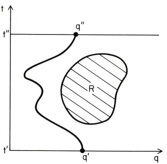
Figure 9: Coarse graining by the behavior of paths with respect to a single spacetime region. The paths which pass between $q^{\prime}$ at time $t^{\prime}$ and $q^{\prime\prime}$ at time $t^{\prime\prime}$ may be partitioned into two classes. First, the class of all paths which never cross the region $R$ one of which is illustrated. Second, the class of paths which intersect $R$ sometime, generally more than once. This partition defines a set of spacetime alternatives for the particle which are not at a moment of time.

In his original paper on the sum-over-histories formulation of quantum mechanics, Feynman Fey48 discussed alternatives defined by spacetime regions such as we have described above. In particular, he offered a sum-over-histories prescription for the probability that “if an ideal measurement is performed to determine whether a particle has a path lying in a region of spacetime…the result will be affirmative”. However, that discussion, as well as more recent ones Men79 , Cav86 , Cav87 , Sch87 , Har88a , Sor89 , and YT91a , were incomplete because they did not specify precisely what such an ideal measurement consisted of or what was to replace the reduction of the state vector following its completion. It is possible to incorporate spacetime alternatives in a generalized non-relativistic quantum mechanics in which “measurement” does not play a fundamental role. We now specify more precisely the three elements — fine-grained histories, allowed coarse grainings and decoherence functional — for such a generalized sum-over-histories quantum mechanics of the closed, non-relativistic models we shall consider.

We consider systems described by an $\nu$-dimensional configuration space ${\bf R}^{\nu}$. The fine-grained histories are paths in this configuration space parametrized by the physical time $t$ between times $t=0$ and $t=T$. We denote the paths by $q(t)$ or by $(q^{1}(t),q^{2}(t),\cdots,q^{\nu}(t))$ when it is necessary to specify the individual coordinates. A defining feature of a non-relativistic system is that its fine-grained histories are single-valued functions of the physical time — one and only one $q$ for each value of $t$. It is a characteristic feature of sum-over-histories formulations of quantum mechanics that a unique most fine-grained set of histories is assumed. In this case it is the set of paths in configuration space.

The allowed coarse-grainings are any partition of the class $u$ of all paths on the time interval $[0,T]$ into an exhaustive set of exclusive classes $\{c_{\alpha}\}$.

$$\cup_{\alpha}c_{\alpha}=u\ ,\qquad\qquad c_{\alpha}\cap c_{\beta}=\phi\ ,\quad\alpha\not=\beta\,.$$ (140)

The central element is the decoherence functional for the set of alternative coarse-grained histories $\{c_{\alpha}\}$. Since we are constructing a sum-over-histories formulation with a unique most fine-grained set of histories (the particle paths) we could proceed by simply writing down the decoherence functional for this fine-grained set. Decoherence functionals for coarse-grained sets are superpositions of this [cf. (IV.1.1iv)]. However, for better analogy with later models we begin by constructing the class operators that are the analogs for spacetime coarse grainings of the chains of projections (14) that represent sequences of alternatives at definite moments of time.

The class operator $C_{\alpha}$ corresponding to a coarse-grained history $c_{\alpha}$ is defined by giving its matrix elements:

$$\left\langle q^{\prime\prime}\left|C_{\alpha}\right|q^{\prime}\right\rangle=\int_{[q^{\prime}\alpha q^{\prime\prime}]}\delta q\,e^{iS[q(\tau)]/\hbar}$$ (141)

where the sum is over all paths in the class $c_{\alpha}$ that start at $q^{\prime}$ at time $t=0$ and end at $q^{\prime\prime}$ and time $T$. The class operators incorporate the dynamics specified by the action $S[q(\tau)]$. We assume this is of standard non-relativistic form:

$$S[q(\tau)]=\int^{T}_{0}dt\ \left[{\cal T}(\dot{q})-V(q)\right]\,,$$ (142)

where ${\cal T}$ is the kinetic energy quadratic form

$${\cal T}(V)={\textstyle{1\over 2}}\sum\nolimits^{\nu}_{i=1}M_{i}(V^{i})^{2}\ .$$ (143)

We shall return shortly to the mathematical definition of path integrals like (141) including the specification of the “measure”. For the moment, we note a few consequences of the definition of class operators. If $\{c_{\bar{\alpha}}\}$ is any coarse graining of the set $\{c_{\alpha}\}$ so that

$$c_{\bar{\alpha}}=\cup_{\alpha\epsilon\bar{\alpha}}\ c_{\alpha}\quad,\quad c_{\bar{\alpha}}\cap c_{\bar{\beta}}=0,\,\bar{\alpha}\not=\bar{\beta}\,,$$ (144)

then it follows immediately from the linearity of the integral in (141) that

$$C_{\bar{\alpha}}=\sum\limits_{\alpha\epsilon\bar{\alpha}}C_{\alpha}\,.$$ (145)

If we completely coarse grain, then we have

$$\left\langle q^{\prime\prime}|C_{u}|q^{\prime}\right\rangle=\sum\nolimits_{\alpha}\left\langle q^{\prime\prime}\left|C_{\alpha}\right|q^{\prime}\right\rangle=\int_{[q^{\prime},q^{\prime\prime}]}\delta q\,e^{iS[q(\tau)]/\hbar}$$ (146)

where the integral is over the class of all the paths $q(t)$ between $q^{\prime}$ at $t=0$ and $q^{\prime\prime}$ at $t=T$. This is the propagator between $t=0$ and $t=T$ [cf. (57)]. Thus, we have

$$\sum\nolimits_{\alpha}C_{\alpha}=e^{-iHT/\hbar}\,.$$ (147)

The result (147) points to a difference in normalization between the class operators defined by (141) and the chains of Heisenberg picture projections, e.g. (14), used in the preceding sections. The latter add to unity when summed over all alternatives while the $C_{\alpha}$’s of this section add to the unitary evolution operator over the time interval $T$. In dealing with path integrals, the Schrödinger picture is more natural than the Heisenberg one, and as a result the normalization (147) is more convenient. The normalization, however, is only a convention and we could restore the Heisenberg picture normalization by multiplying all $C$’s by $\exp(iHT)$.

To construct the decoherence functional $D(\alpha^{\prime},\alpha)$ we must specify not only the class operators but also initial and final conditions. In this non-relativistic example, an initial condition is specified by giving a family of orthonormal wave functions $\{\psi_{j}(q)\}$ in the Hilbert space ${\cal H}$ of square integrable functions on ${\bf R}^{\nu}$ together with their probabilities $\{p^{\prime}_{j}\}$. Equivalently and more compactly, we can summarize the initial condition by the density matrix

$$\rho_{i}\left(q^{\prime}_{0},q_{0}\right)=\sum_{j}\psi_{j}\left(q^{\prime}_{0}\right)p_{j}\psi^{*}_{j}\left(q_{0}\right)\,.$$ (148)

A final condition is similarly specified by a family of orthonormal wave functions $\{\phi_{i}(q)\}$ and their probabilities $\{p^{\prime\prime}_{i}\}$ or equivalently by a final density matrix $\rho_{f}$.

Initial and final conditions are adjoined to the class operators by the usual inner product in ${\cal H}$

$$\left\langle\phi_{i}\left|C_{\alpha}\right|\psi_{j}\right\rangle = \int dq^{\prime\prime}\int dq^{\prime}\phi^{*}_{i}\left(q^{\prime\prime}\right)\left\langle q^{\prime\prime}\left|C_{\alpha}\right|q^{\prime}\right\rangle\psi_{j}\left(q^{\prime}\right)$$ (149)

$$= \int_{\alpha}\delta q\,\phi^{*}_{i}\left(q^{\prime\prime}\right)\,e^{iS[q(\tau)]/\hbar}\,\psi_{j}\left(q^{\prime}\right)$$

where in the second line of (149) we understand the path integral to include an integration over the endpoints $q^{\prime}$ and $q^{\prime\prime}$.

We now define the decoherence functional $D(\alpha^{\prime},\alpha)$ by:

$$D\left(\alpha^{\prime},\alpha\right) = {\cal N}\sum_{ij}p^{\prime\prime}_{i}\left\langle\phi_{i}\left|C_{\alpha^{\prime}}\right|\psi_{j}\right\rangle p^{\prime}_{j}\left\langle\psi_{j}\left|C_{\alpha}\right|\phi_{i}\right\rangle$$ (150a)

$$= {\cal N}\,Tr\left[\rho_{f}C_{\alpha^{\prime}}\rho_{i}C^{\dagger}_{\alpha}\right]$$ (150b)

where

$${\cal N}^{-1}=Tr\left[\rho_{f}e^{-iHT}\rho_{i}e^{iHT}\right]\,.$$ (150c)

Equation (150) is the same as (139) but using Schrödinger picture representatives of the initial and final conditions rather than Heisenberg ones.

It is straightforward to verify that the decoherence functional defined by (150) satisfies the four requirements (117) of a decoherence functional of a generalized quantum mechanics. It is Hermitian because $\rho_{i}$ and $\rho_{f}$ are Hermitian, and positive because they are positive. It is normalized because of (147). It obeys the superposition principle because of (145).

The generalized quantum mechanics we have just constructed appears to depend explicitly on the time interval $T$. Paths were considered on the time interval $[0,T]$ and the class operators and decoherence functional depend explicitly on its length. However, any partition of the paths on the interval $[0,T]$ is also trivially a partition of the paths on a longer interval $[0,\widetilde{T}]$, $\widetilde{T}\geq T$. The class operators are related by

$$\widetilde{C}_{\alpha}=e^{-iH(\widetilde{T}-T)/\hbar}\,C_{\alpha}\,.$$ (151)

If the final density matrix at $\widetilde{T}$ is related to that at $T$ by Schrödinger evolution

$$\tilde{\rho}_{f}=e^{-iH(\widetilde{T}-T)/\hbar}\,\rho_{f}e^{iH(\widetilde{T}-T)/\hbar}\,,$$ (152)

then the decoherence functional is independent of $\widetilde{T}$. A similar argument shows independence of the time of the initial condition, provided $\rho_{i}$ evolves according to the Schrödinger equation.

We have given the decoherence functional in its general time-neutral form with both initial and final conditions. As discussed in Section IV.7, a final condition of indifference with respect to final state, $\rho_{f}=I$, is likely to be an accurate representation of the final condition of our universe. In that case the decoherence functional takes the more familiar form

$$D\left(\alpha^{\prime},\alpha\right)=Tr\bigl{[}C_{\alpha^{\prime}}\rho C^{\dagger}_{\alpha}\bigr{]}$$ (153)

where $\rho_{i}=\rho$ is a normalized density matrix representing the initial condition.

The generalized sum-over-histories, non-relativistic quantum mechanics we have just constructed is in fully spacetime form. Dynamics are expressed as a sum-over-fine-grained-spacetime histories involving an action functional of these histories and coarse-grained alternatives are defined by spacetime partitions of these histories. The class of alternatives considered by this generalized quantum mechanics is thus greatly enlarged beyond the usual alternatives at definite moments of time. It is this extension of the “observables” that will be important in constructing quantum mechanics for theories where there is no well defined notion of time. In the following we shall illustrate some of these more general spacetime alternatives explicitly in non-relativistic quantum mechanics. First, however, we consider how to define the path integrals involved.

V.2 Evaluating Path Integrals

V.2.1 Product Formulae

We are interested in the path integrals that define the class operators of the form

$$\left\langle\phi_{i}\left|C_{\alpha}\right|\psi_{j}\right\rangle=\int_{\alpha}\delta q\,\phi^{*}_{i}\left(q^{\prime\prime}\right)e^{iS[q(\tau)]}\psi_{j}\left(q^{\prime}\right)\,,$$ (154)

units having been chosen for this and subsequent sections so that $\hbar=1$. How are they defined and how do we compute them?

General arguments Cam60 show that it is not possible to introduce a complex measure on the space of paths to define the Feynman integral. However, path integrals may be defined and computed by other means DMN79 . Here, we take the point of view, introduced by Feynman Fey48 , that expressions like (154) are to be defined by the limits of their values on polygonal (skeletonized) paths on a time slicing of the interval $[0,T]$. Suppose that this interval is divided into $N$ sub-intervals of equal length $\epsilon=T/N$ with boundaries at $t_{0}=0,t_{1},t_{2},\cdots,t_{N}=T$. A polygonal path is specified by giving the values $(q_{0},\cdots,q_{N})$ of $q(t)$ on the $N+1$ time slices including the value $q_{0}(\equiv q^{\prime})$ at the initial time $t=0$ and the value $q_{N}$ $(\equiv q^{\prime\prime})$ at the final time $t_{N}=T$. The polygonal paths consist of straight line segments joining the points $(q_{0},\cdots,q_{N})$ at the times defining the subdivision. The non-relativistic action (142) is straightforwardly evaluated on polygonal paths when the spacing $\epsilon$ is small.

$$S(q_{N},\cdots,q_{0})\approx\sum\limits^{N-1}_{k=0}\epsilon\Biggl{[}{\cal T}\biggl{(}\frac{q_{k+1}-q_{k}}{\epsilon}\biggr{)}-V(q_{k})\Biggr{]}\,.$$ (155)

Any partition of continuous paths will also partition the polygonal paths. Let $e_{\alpha}(q_{N},\cdots,q_{0})$ be the function which is unity on all polygonal paths in the class $c_{\alpha}$ and zero otherwise. Then, with these preliminaries, we define an expression like (154) as the following limit

$$\left\langle\phi_{i}\left|C_{\alpha}\right|\psi_{j}\right\rangle=\lim\limits_{N\to\infty}\int dq_{N}\int dq_{N-1}\cdots\int dq_{0}\ \mu(N)$$

$$\times\phi^{*}_{i}(q_{N})e_{\alpha}(q_{N},\cdots,q_{0})e^{iS(q_{N},\cdots,q_{0})}\psi_{j}(q_{0})\,.$$ (156)

where $\mu(N)$ is an $N$-dependent constant “measure” factor and the integrals are all over ${\bf R}^{\nu}$.

The definition (156) is not, by itself, a computationally effective way of evaluating Feynman integrals. Operator methods provide a more efficient tool. As was first recognized by Nelson Nel64 , operator product formulae provide both a way of demonstrating the existence of limits like (156) and of evaluating the class operators $C_{\alpha}$ to which they correspond. As the most familiar example, consider the propagator which is the path integral (154) evaluated over the class, $u$, of all paths on the time interval $[0,T]$. Then $e_{\alpha}=1$. Divide the total Hamiltonian $H$ following from the action (142) into a free part $H_{0}$ corresponding to the kinetic energy ${\cal T}$ and the potential $V$:

$$H=\sum\nolimits^{\nu}_{i=1}\frac{p^{2}_{i}}{2M_{i}}+V(q^{k})\equiv H_{0}+V\,.$$ (157)

The propagator for the free part of the Hamiltonian is an elementary calculation,

$$\langle q^{\prime\prime}|e^{-iH_{0}t}|q^{\prime}\rangle=F(t)\exp\Biggl{[}it{\cal T}\biggl{(}\frac{q^{\prime\prime}-q^{\prime}}{t}\biggr{)}\Biggr{]}\,,$$ (158)

where

$$F(t)=\prod\limits^{\nu}_{i=1}(M_{i}/2\pi it)^{\textstyle{1\over 2}}\,.$$ (159)

It follows that, if the constant $\mu$ in (156) happens to be $[F(\epsilon)]^{N}$, then we can write

$$\left\langle\phi_{i}\left|C_{\alpha}\right|\psi_{j}\right\rangle=\lim\limits_{N\to\infty}\langle\phi_{i}|\Bigl{(}e^{-iH_{0}(T/N)}\ e^{-iV(T/N)}\Bigr{)}^{N}|\psi_{j}\rangle\,.$$ (160)

This fixes the “measure” in the path integral. If $H_{0}$ and $V$ are densely defined, self-adjoint and bounded from below, the Trotter product formula Tro59 states

$$\lim\limits_{N\to\infty}\Bigl{(}e^{-iH_{0}(T/N)}\ e^{-iV(T/N)}\Bigr{)}^{N}=e^{-i(H_{0}+V)T}\,.$$ (161)

Thus, the limit in (156) exists, and the path integral $\left\langle\phi_{i}\left|C_{\alpha}\right|\psi_{j}\right\rangle$ is evaluated as

$$\left\langle\phi_{i}\left|C_{\alpha}\right|\psi_{j}\right\rangle=\langle\phi_{i}|e^{-iHT}|\psi_{j}\rangle\,.$$ (162)

The relation (162) is hardly a surprise. It is the path integral expression for the propagator originally derived by Feynman Fey48 .

From this perspective formulating quantum mechanics in terms of path integrals does not eliminate the need for Hilbert space. Indeed, a Hilbert space is central to the product formulae approach to defining path integrals. In non-relativistic quantum mechanics, the Hilbert space used to define path integrals coincides with the Hilbert space of states on a constant time surface. In general, however, we shall see that there is no such connection, not least because it is not always possible to define states on a spacelike surface.

V.2.2 Phase-Space Path Integrals

In (160) we used a product formula to fix the “measure” factors (159) in the path integral. Evaluated in a different way, the product formula can be interpreted as an integral over phase space paths which gives a more convenient and physically suggestive way of summarizing these factors. As such phase-space path integrals are a natural way of fixing the measure in the generalizations of quantum mechanics we shall consider later we briefly pause to consider such integrals here.

We recover the Lagrangian path integral for $C_{u}$ [Eq. (156) with $e_{u}=1$] if the resolution of the identity

$$I=\int dq|q\rangle\,\langle q|$$ (163)

is inserted between each factor of the product in (160) and (158) is used to evaluate the matrix elements involving $H_{0}$. The same procedure used with the resolution

$$I = \frac{1}{2\pi}\int dp\,dq|q\rangle\,\langle q|p\rangle\,\langle p|$$ (164)

$$= \frac{1}{2\pi}\int dp\,dq\,e^{ip\cdot q}|q\rangle\,\langle p|$$

yields the phase-space path integral. The matrix elements are immediate since $H_{0}$ is diagonal in $p_{k}$ and $V$ is diagonal in $q^{k}$. The result for the configuration space matrix elements of $C_{u}$ is the limit.

$$\langle q^{\prime\prime}|C_{u}|q^{\prime}\rangle=\langle q^{\prime\prime}|e^{-iHT}|q^{\prime}\rangle=\lim_{N\to\infty}\int\frac{dp_{N}}{2\pi}\prod^{N-1}_{k=1}\left(\frac{dp_{k}dq_{k}}{2\pi}\right)$$

$$\times\exp\Biggl{[}i\sum^{N}_{J=1}\epsilon\left\{p_{J}\cdot\left(\frac{q_{J}-q_{J-1}}{\epsilon}\right)-\Bigl{[}H_{0}\left(p_{J}\right)+V\left(q_{J-1}\right)\Bigr{]}\right\}\Biggr{]}\,.$$ (165)

Here, of course, $p\cdot q=p_{i}q^{i}\ ,\ H_{0}(p)$ is the function defined by (157), and $dp$ and $dq$ represent the usual volume elements on the $\nu$-dimensional momentum and configuration spaces respectively. The limit (165) defines the phase-space path integral

$$\left\langle q^{\prime\prime}\left|C_{u}\right|q^{\prime}\right\rangle=\int\delta p\,\delta q\,\exp\left[i\int^{T}_{0}dt\,\Bigl{[}p\cdot(dq/dt)-H(p,q)\Bigr{]}\right]\,.$$ (166)

The phase-space path integral (166) has been discussed by many authors, e.g. Fey51 and Gar66 . The construction can be extended to define the $C_{\alpha}$’s for finer configuration space coarse grainings simply by restricting the $q$-integral to the class of paths $\{c_{\alpha}\}$. It can also be extended to incorporate momentum coarse-grainings (see, e.g. GH93 ). The interpretation of (166) as an integral is not as straightforward as in the Lagrangian case. Among other things, the momentum space paths are discontinuous.

For our purposes, the utility of the phase-space path integral is that it provides a physically transparent way of summarizing the “measure” in the path integral and a way of computing that measure in more general cases. The measure in (165) is the canonical, Liouville measure in phase-space “$dpdq/(2\pi\hbar)$”. Since the momentum space integrals like (165) are unconstrained even when the configuration space ones are restricted by a coarse graining, the Gaussian integrals over the $p^{i}_{J}$ can be carried out explicitly. The result is the Lagrangian path integral (156) over configuration space paths including the correct “measure” factor $[F(T/N)]^{N}$ with $F$ given by (159).

V.3 Examples of Coarse Grainings

V.3.1 Alternatives at Definite Moments of Time

The most familiar type of coarse graining is by regions of configuration space at successive moments of time (see Figure 10) described briefly in Section IV.3. Suppose, for example, we consider sets of exhaustive non-overlapping regions of ${\bf R}^{\nu}$, $\{\Delta^{1}_{\alpha_{1}}\}$, $\{\Delta^{2}_{\alpha_{2}}\}$, $\cdots$, $\{\Delta^{n}_{\alpha_{n}}\}$ at a discrete series of times $t_{1},\cdots,t_{n}$. At each time $t_{k}$

$$\cup_{\alpha_{k}}\Delta^{k}_{\alpha_{k}}={\bf R}^{\nu}\ ,\qquad\qquad\Delta^{k}_{\alpha_{k}}\cap\Delta^{k}_{\beta_{k}}=\phi\ ,\quad\alpha_{k}\not=\beta_{k}\,.$$ (167)

Since the paths are single valued in time, they pass through one and only one region at each of the instants $t_{k}$. The class of all paths may be partitioned into all possible ways they cross these regions. Coarse grained histories are thus labeled by the particular sequence of regions $\Delta^{1}_{\alpha_{1}},\cdots,\Delta^{n}_{\alpha_{n}}$ at times $t_{1},\cdots,t_{n}$. We write them as $c_{\alpha_{n}\cdots\alpha_{1}}$. The individual coarse-grained history $c_{\alpha_{n}\cdots\alpha_{1}}$ corresponds to the particle being localized in region $\Delta^{1}_{\alpha_{1}}$ at time $t_{1}$, $\Delta^{2}_{\alpha_{2}}$ at time $t_{2}$ and so forth.

The class operators $C_{\alpha}$ for coarse grainings defined by alternative spatial regions at definite moments of time are readily evaluated by the techniques of the last subsection. The integrals in (141) are restricted to the ranges $\Delta^{1}_{\alpha_{1}},\cdots,\Delta^{n}_{\alpha_{n}}$ on the slices $t_{1},\cdots,t_{n}$. The corresponding product formula analogous to (160) will consist of unitarity evolution in between these times interrupted by projections on these ranges at them. Thus if $\alpha=(\alpha_{n},\cdots,\alpha_{1})$ denotes the coarse-grained history in which the paths pass through regions $\Delta^{1}_{\alpha_{1}},\cdots,\Delta^{n}_{\alpha_{n}}$ at times $0\leq t_{1}\leq t_{2}\leq\cdots\leq t_{n}\leq T$, then

$$C_{\alpha}=e^{-iH(T-t_{n})}P^{n}_{\alpha_{n}}e^{-iH(t_{n}-t_{n-1})}P^{n-1}_{\alpha_{n-1}}\cdots P^{1}_{\alpha_{1}}e^{-iHt_{1}}$$ (168)

where $P^{k}_{\alpha_{k}}$ is the projection on the configuration space region $\Delta^{k}_{\alpha_{k}}$ at time $t_{k}$. The expression is more compact with Heisenberg picture operators

$$C_{\alpha}=e^{-iHT}P^{n}_{\alpha_{n}}(t_{n})\cdots P^{1}_{\alpha_{1}}(t_{1})\,.$$ (169)

This is enough to show that the $C_{\alpha}$ in general will neither be unitary nor Hermitian. Neither is it true that $C_{\alpha}C_{\beta}=0$ for distinct histories. The relations (167) expressing the conditions that the regions of configuration space are exhaustive and exclusive at each time translate into

$$\sum\nolimits_{\alpha_{k}}P^{k}_{\alpha_{k}}(t_{k})=1,\quad P^{k}_{\alpha_{k}}(t_{k})P^{k}_{\alpha^{\prime}_{k}}(t_{k})=\delta_{\alpha_{k}\alpha^{\prime}_{k}}P^{k}_{\alpha_{k}}(t_{k})\,.$$ (170)

These are enough to show explicitly that (157) is satisfied and further that

$$\sum\nolimits_{\alpha}C^{\dagger}_{\alpha}C_{\alpha}=I$$ (171)

for this particular class of coarse grainings. Thus, we recover from the sum-over-histories formulation the usual Hamiltonian expressions for the class operators of this kind of coarse graining [cf. (14) with appropriate change in normalization].

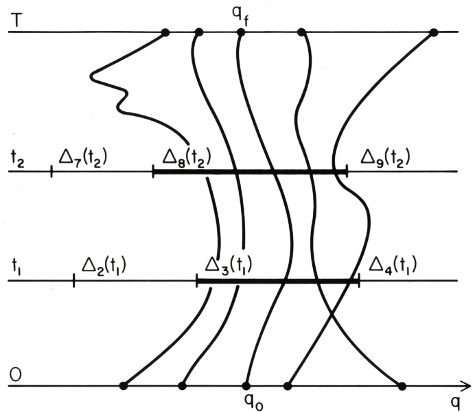
Figure 10: Coarse graining by regions of configuration space at successive moments of time. The figure shows a spacetime that is a product of a one-dimensional configuration space $(q)$ and the time interval $[0,T]$. At times $t_{1}$ and $t_{2}$ the configuration space is divided into exhaustive sets of non-overlapping intervals: $\{\Delta^{1}_{\alpha_{1}}\}$ at time $t_{1}$, and $\{\Delta^{2}_{\alpha_{2}}\}$ at time $t_{2}$. Some of these intervals are illustrated. (The superscripts have been omitted from the $\Delta$’s for compactness.) The fine-grained histories are the paths which pass between $t=0$ and $t=T$. Because the paths are assumed to be single-valued in time, the set of fine-grained histories may be partitioned according to which intervals they pass through at times $t_{1}$ and $t_{2}$. The figure illustrates a few representative paths in the class $c_{83}$ which pass through region $\Delta^{1}_{3}$ at time $t_{1}$ and region $\Delta^{2}_{8}$ at time $t_{2}$.

V.3.2 Alternatives Defined by a Spacetime Region

Coarse grainings by spatial regions at definite moments of time are only a very special case of the coarse grainings that are possible in sum-over-histories quantum mechanics. As an example of a more general coarse grainings we consider partitions of the paths according to their behavior with respect to a spacetime region $R$ (Figure 9).

Given a spacetime region $R$, the paths between $t=0$ and $t=T$ may be partitioned into two exclusive classes: (1)  The class $\bar{r}$ of all paths that never intersect $R$, and (2)  the class $r$ of paths that intersect $R$ at least once. To evaluate the corresponding class operators we begin with the path integral over the class $c_{\bar{r}}$

$$\left\langle\phi_{i}\left|C_{\bar{r}}\right|\psi_{j}\right\rangle=\int\nolimits_{\bar{r}}\delta q\ \phi^{*}_{i}(q^{\prime\prime})\,\exp\bigl{(}iS[q(\tau)])\psi_{j}(q^{\prime})\,.$$ (172)

The Feynman integral is the limit of the integral over polygonal paths in $\bar{r}$ as in (156). Each constant-time cross section of $R$ is a region of configuration space $\Delta(t)$. The paths of $\bar{r}$ lie entirely in the complements of these regions, $\bar{\Delta}(t)$. By introducing projection operators on the regions $\bar{\Delta}$ at the various times, the integrals over polygonal paths defining (172) may be expressed as matrix elements of operators. Let $P_{\bar{\Delta}(t)}$ denote the projection onto the complement of $\Delta(t)$. $P_{\bar{\Delta}(t)}$ is time dependent, not because it is a Heisenberg picture operator, but because the region $\bar{\Delta}(t)$ is time dependent. Clearly

$$<q^{\prime\prime}|P_{\bar{\Delta}}|q^{\prime}>=\delta(q^{\prime\prime}-q^{\prime})e_{\bar{\Delta}}(q^{\prime})\ .$$ (173)

Using this and the free propagator, (158), the path integral over the class $\bar{r}$ can be written as the limit

$$\left\langle\phi_{i}\left|C_{\bar{r}}\right|\psi_{j}\right\rangle=\lim\limits_{N\to\infty}<\phi_{i}|{\bf T}\prod\limits^{N-1}_{k=0}\Biggl{(}e^{-iH_{0}(T/N)}e^{-iV(T/N)}P_{\bar{\Delta}(kT/N)}\Biggr{)}|\psi_{j}>$$ (174)

where the product is time ordered — written with the earliest $P_{\bar{\Delta}(t)}$’s to the right. The projection, $P_{\bar{\Delta}(t)}$ can be written in the form

$$P_{\bar{\Delta}(t)}=e^{-E_{R}(t)\epsilon}$$ (175)

where $\epsilon$ is an arbitrary positive number and $E_{R}$ is the excluding potential for the spacetime region $R$, that is

$$E_{R}(q,t)=\left\{\begin{array}[]{lr}0&(q,t)\ \notin\ R\,,\\ +\infty&(q,t)\ \in\ R\,.\end{array}\right.$$

Choosing $\epsilon=T/N$ we may then write (174) as

$$\left\langle\phi_{i}\left|C_{\bar{r}}\right|\psi_{j}\right\rangle=<\phi_{i}|\lim\limits_{N\to\infty}{\bf T}\prod\limits^{N-1}_{k=0}\Biggl{(}e^{-iH_{0}(T/N)}e^{-i(V-iE_{R}(kT/N))(T/N)}\Biggr{)}|\psi_{j}>\,.$$ (176)

Again, the operators in (176) are time ordered with the earliest on the right.

As a generalization of the Trotter product formula (161) we expect

$$\lim\limits_{N\to\infty}{\bf T}\prod\limits^{N-1}_{k=0}\left(e^{-iH_{0}(T/N)}e^{-i(V-iE_{R}(kT/N))(T/N)}\right)$$

$$={\bf T}\exp\biggl{\{}-i\int\nolimits^{T}_{0}dt\bigl{[}H_{0}+V-iE_{R}(t)\bigr{]}\biggr{\}}$$ (177)

where ${\bf T}$ denotes the time ordered product. That is, the right hand side of (177) may be interpreted as $U_{R}(T)$ where $U_{R}(t)$ is the solution of

$$i\frac{dU_{R}(t)}{dt}=\left[H_{0}+V-iE_{R}(t)\right]U_{R}(t)\,,$$ (178)

with the boundary condition

$$U_{R}(0)=I\,.$$ (179)

Physically (178) represents Schrödinger evolution in the presence of a completely absorbing potential on the spacetime region $R$. Paths that once cross into the region $R$ do not contribute to the final value of $U$.

Equation (177) allows us to identify the class operators for the coarse graining based on a single spacetime region, $R$. There are two coarse-grained histories in the set: $r$, the class of fine-grained histories which cross $R$ at least once and $\bar{r}$, class of the fine-grained histories which never cross $R$. For $\bar{r}$ we have

$$C_{\bar{r}}=U_{R}(T)={\bf T}\exp\biggl{\{}-i\int\nolimits^{T}_{0}dt\left[H_{0}+V-iE_{R}(t)\right]\biggr{\}}\,.$$ (180)

The operator $C_{r}$ then follows from the fact that the set of paths $r$ which cross $R$ at least once is the difference between the set of all paths $u$ and the set which $\bar{r}$ which never cross $R$:

$$r=u-\bar{r}$$ (181)

where, as usual, $a-b\equiv a\cap\bar{b}$. The corresponding relation for the class operators is

$$C_{r}=e^{-iHT}-U_{R}(T)\,,$$ (182)

which is the same as (147).

V.3.3 A Simple Example of a Decoherent Spacetime Coarse Graining

Consider a free particle in one dimension and let the region $R$ be the whole region $x<0,\;0<t<T$. Then $C_{\bar{r}}$ is just the evolution operator in the presence of an infinite potential wall at $q=0$, that is

$$<q^{\prime\prime}|C_{\bar{r}}|q^{\prime}>=\theta(q^{\prime\prime})\theta(q^{\prime})\biggl{(}\frac{M}{2\pi iT}\biggr{)}^{\textstyle{1\over 2}}$$

$$\times\Biggl{\{}\exp\left[i\frac{M}{2T}(q^{\prime\prime}-q^{\prime})^{2}\right]-\exp\left[i\frac{M}{2T}(q^{\prime\prime}+q^{\prime})^{2}\right]\Biggr{\}}\,.$$ (183)

From (182) the position matrix elements of $C_{r}$ are the free propagator minus (183) or

$$<q^{\prime\prime}|C_{r}|q^{\prime}>=\Bigl{[}\theta(q^{\prime\prime})\ \theta(-q^{\prime})+\theta(-q^{\prime\prime})\theta(q^{\prime})\Bigr{]}\left(\frac{M}{2\pi iT}\right)^{\textstyle{1\over 2}}\exp\Bigl{[}i\frac{M}{2T}(q^{\prime\prime}-q^{\prime})^{2}\Bigr{]}$$

$$+\bigl{[}\theta(q^{\prime\prime})\theta(q^{\prime})+\theta(-q^{\prime\prime})\theta(-q^{\prime})\bigr{]}\left(\frac{M}{2\pi iT}\right)^{\textstyle{1\over 2}}\exp\left[i\frac{M}{2T}(q^{\prime\prime}+q^{\prime})^{2}\right]\,.$$ (184)

Special choices of the initial condition can give examples in which the alternatives $r$ and $\bar{r}$ are decoherent. Such examples have been investigated especially by Yamada and Takagi YT91b . A simple case is obtained by considering a pure initial state with a wave function $\psi(x)$. Write this as

$$\psi(x)=\alpha\,\phi_{+}(x)+\beta\,\phi_{-}(x)\ ,\qquad\ \left|\alpha\right|^{2}+\left|\beta\right|^{2}=1\,,$$ (185)

where $\phi_{+}(x)$ and $\phi_{-}(x)$ are normalized wave functions having support on $x>0$ and $x<0$ respectively. The branch wave functions corresponding to the alternatives $r$ and $\bar{r}$ may be expressed in terms of the free unitary evolution operator for the time interval $T$ which we denote by $U$. Thus, for example, the branch, $\psi_{\bar{r}}$, representing the alternative that the particle never crosses into $x<0$ in the time interval $T$ is

$$\psi_{\bar{r}}(x)=\alpha P_{+}\bigl{[}U\phi_{+}(x)-U\phi_{+}(-x)\bigr{]}$$ (186)

where $P_{+}$ is the projection onto $x>0$. Eq. (186) is just the usual “method of images” solution of the Schrödinger equation is the presence of an infinite barrier at $x=0$ and is another way of writing (183).

The other branch is

$$\psi_{r}(x)=U\psi(x)-\psi_{\bar{r}}(x)\,.$$ (187)

The condition for decoherence is

$$\left(\psi_{r},\psi_{\bar{r}}\right)=0\,.$$ (188)

Evidently this is a linear relation and $\alpha$ and $\beta$ of the form

$$\alpha c_{+}+\beta c_{-}=0$$ (189)

where $c_{\pm}$ are coefficients completely determined by $\phi_{\pm}$ and $U$. Eq. (189) and the normalization condition (185) fix $\alpha$ and $\beta$.

The probabilities for the decoherent set of alternatives may also be expressed directly in terms of $c_{\pm}$. We have

$$p_{r}=\left(\psi_{r},\psi_{r}\right) = c^{2}_{+}/\bigl{(}c^{2}_{+}+c^{2}_{-}\bigr{)}\,,$$ (190a)

$$p_{\bar{r}}=\left(\psi_{\bar{r}},\psi_{\bar{r}}\right) = c^{2}_{-}/\bigl{(}c^{2}_{+}+c^{2}_{-}\bigr{)}\,.$$ (190b)

It is not difficult to be convinced that, by different choices of $\phi_{\pm}$, examples of the whole range of possible probabilities may be obtained. An especially simple example is to take YT91b

$$\phi_{+}(x)=-\phi_{-}(-x)$$ (191)

and $\alpha=\beta=1/\sqrt{2}$. Then, for any $\phi_{-}(x)$ decoherence is exact and $p_{r}=p_{\bar{r}}=1/2$ — both results which alternatively follow from symmetry considerations.

These examples show that decoherence of spacetime coarse grainings can be achieved in special examples and that these alternatives can have non-trivial probabilities.

V.4 Coarse Grainings by Functionals of the Paths

V.4.1 General Coarse Grainings

The most general notion of coarse graining is given by partitions of the paths by ranges of values of functionals of the paths. Several functionals are possible but for simplicity we shall just consider one. Denote it by $F[q(\tau)]$ and consider an exhaustive set of intervals $\{\Delta_{\alpha}\}$ of the real line. The class $c_{\alpha}$ consists of those paths for which $F[q(\tau)]$ lies in the interval $\Delta_{\alpha}$

$$c_{\alpha}=\bigl{\{}q(t)\big{|}F[q(\tau)]\epsilon\Delta_{\alpha}\bigr{\}}\,.$$ (192)

This is the most general notion of coarse graining because, given any partition of the paths into classes $\{c_{\alpha}\}$, we could always take $F$ to be the function that is $\alpha$ if the path is in class $c_{\alpha}$ and take $\{\Delta_{\alpha}\}$ to be unit intervals surrounding the integers.

The class operators $C_{\alpha}$ corresponding to the classes $c_{\alpha}$ are defined, as always, by

$$\left\langle\phi_{i}\left|C_{\alpha}\right|\psi_{j}\right\rangle=\int\nolimits_{\alpha}\delta q\,\phi^{*}_{i}(q^{\prime\prime})\exp\bigl{(}iS[q(\tau)]\bigr{)}\psi_{j}(q^{\prime})\,.$$ (193)

They can be evaluated by introducing the characteristic functions for the intervals $\Delta_{\alpha}$ on the real line:

$$e_{\alpha}(x)=\left\{\begin{array}[]{rl}1&x\in\Delta_{\alpha}\,,\\ 0&x\notin\Delta_{\alpha}\,,\end{array}\right.$$

and their Fourier transforms $\tilde{e}_{\alpha}(\mu)$

$$e_{\alpha}(x)=\int^{+\infty}_{-\infty}d\mu\,e^{i\mu x}\tilde{e}_{\alpha}(\mu)\,.$$ (194)

Then, clearly

$$\left\langle\phi_{i}\left|C_{\alpha}\right|\psi_{j}\right\rangle=\int^{+\infty}_{-\infty}d\mu\,\tilde{e}_{\alpha}(\mu)\int\nolimits_{u}\delta q\,\phi^{*}_{i}(q^{\prime\prime})\,\exp\biggl{\{}i\Bigl{(}S[q(\tau)]+\mu F[q(\tau)]\Bigr{)}\biggr{\}}\psi_{j}(q^{\prime})\,.$$ (195)

When $F[q(\tau)]$ is a local functional, that is of the form

$$F[q(\tau)]=\int\nolimits^{T}_{0}dtf\left(\dot{q}(t),q(t),t\right)\,,$$ (196)

then there is an effective Hamiltonian $H_{F}(t,\mu)$ associated with the effective action $S+\mu F$. Quantum mechanically it may be difficult to determine the operator ordering of (196) that reproduces the path integral (195) if one exists at all. However, when this can be done the class operators may be expressed formally as

$$C_{\alpha}=\int^{+\infty}_{-\infty}d\mu\,\tilde{e}_{\alpha}(\mu){\bf T}\exp\Bigl{[}-i\int\nolimits^{T}_{0}H_{F}(t,\mu)dt\Bigr{]}\,.$$ (197)

Equations (195) and (197) are powerful tools for the evaluation of the class operators of the most general sum-over-histories spacetime coarse graining.

It should be stressed that the partitions by values of a functional such as (196) that we have defined here are not the same as partitions by the eigenvalues of the Heisenberg operator corresponding to (196). The class operators for the latter are projections onto ranges of the eigenvalues while the class operators (195) are not projections in general. The two kinds of class operators represent distinct quantum mechanical alternatives that coincide classically – a familiar enough situation. In this sum-over-histories approach to quantum mechanics we shall only consider the path integral partitions of the type we have described.

V.4.2 Coarse Grainings Defining Momentum

We have introduced a large class of spacetime alternatives in the sum-over-histories generalized quantum mechanics of a non-relativistic system. However, we have not mentioned some of the most familiar alternatives of ordinary quantum mechanics, for example, alternative values of momentum at a moment of time. The reason momentum has not been considered is that there is no obvious meaning to a partition of non-differentiable, polygonal, paths by values of $M_{i}\dot{q}^{i}(t)$ at a moment of time. Using the techniques of this section, we can, however, consider partitions by the values of the averages of such derivatives over a time and interval and define momentum with suitable limits of these coarse grainings (cf. FH65 ).

For simplicity, restrict attention to the case of a free particle moving in one dimension. We consider a coarse graining by values of the momentum at time $t$ averaged over a time interval $s$, that is, by values of the functional

$$F_{s}[q(\tau)]=\frac{1}{s}\int\limits^{t+s/2}_{t-s/2}dt^{\prime}M\dot{q}(t^{\prime})=M\left(\frac{q(t+s/2)-q(t-s/2)}{s}\right)\,.$$ (198)

The class operator corresponding to the coarse-grained history in which the value of this averaged momentum lies in a range $\tilde{\Delta}$ is

$$\bigl{\langle}\phi_{i}\bigl{|}C_{\tilde{\Delta}}\bigr{|}\psi_{j}\bigr{\rangle}=\int\delta q\phi^{*}_{i}(q^{\prime\prime})e_{\tilde{\Delta}}\left\{F_{s}[q(\tau)]\right\}\exp\bigl{(}iS[q(\tau)]\bigr{)}\psi_{j}(q^{\prime})$$ (199)

where $e_{\tilde{\Delta}}(x)$ is the characteristic function for the interval $\tilde{\Delta}$ [cf. (V.4.1)]. If we write

$$e_{\tilde{\Delta}}(x)=\int_{\tilde{\Delta}}dp\ \delta(x-p)$$ (200)

then the path integral in (199) is over all paths between $t=0$ and $t=T$ for which the difference in $q$’s in (198) is fixed by $p$. Since the unrestricted path integration between two times generates unitary evolution [cf. (57)], this may be written

$$\bigl{\langle}\phi_{i}\bigl{|}C_{\tilde{\Delta}}\bigr{|}\psi_{j}\bigr{\rangle}=\int\nolimits_{\tilde{\Delta}}dp\int\nolimits^{+\infty}_{-\infty}dq^{\prime}\int\nolimits^{+\infty}_{-\infty}dq^{\prime\prime}\delta\left[M(q^{\prime\prime}-q^{\prime})/s-p\right]$$

$$\times\left\langle\phi_{i}\bigl{|}q^{\prime\prime},t+s/2\right\rangle\left\langle q^{\prime\prime},t+s/2\bigl{|}q^{\prime},t-s/2\right\rangle\left\langle q^{\prime},t-s/2\bigl{|}\psi_{j}\right\rangle\,.$$ (201)

Carry out the integration over $q^{\prime\prime}$ using the $\delta$-function, insert the form of the free propagator from (158), insert complete sets of momentum eigenstates immediately before the final state and after the initial one, and carry out the remaining $q^{\prime}$ integration to find

$$\bigl{\langle}\phi_{i}\bigl{|}C_{\tilde{\Delta}}\bigr{|}\psi_{j}\bigr{\rangle}=s\int\nolimits_{\tilde{\Delta}}dp\int\nolimits^{+\infty}_{-\infty}\frac{dk}{2\pi}\left(\frac{M}{2\pi is}\right)^{\textstyle{1\over 2}}\exp\left[\frac{is}{2M}\ (p-k)^{2}\right]\ \tilde{\phi}^{*}_{i}(k)\tilde{\psi}_{j}(k)$$ (202)

where $\tilde{\phi}_{i}(k)$ and $\tilde{\psi}_{j}(k)$ are the momentum space representatives of the final and initial wave functions respectively.

We examine (202) in the limits of short and long averaging times $s$. As $s\rightarrow 0$, it is evident that

$$\bigl{\langle}\phi_{i}\bigl{|}C_{\tilde{\Delta}}\bigr{|}\psi_{j}\bigr{\rangle}\sim s^{\textstyle{1\over 2}}\,,\ s\rightarrow 0$$ (203)

so that the class operator becomes vacuous! This is another statement of the non-differentiability of the paths. The amplitude to find any finite value for $M\dot{q}(t)$ at a moment of time is zero.

In the limit $s\rightarrow\infty$, the integral in (202) can be evaluated by the method of stationary phase yielding

$$\bigl{\langle}\phi_{i}\bigl{|}C_{\tilde{\Delta}}\bigr{|}\psi_{j}\bigr{\rangle}=\int\nolimits_{\tilde{\Delta}}\frac{dp}{2\pi}\tilde{\phi}^{*}_{i}(p)\psi_{j}(p)=\int\nolimits_{\tilde{\Delta}}\frac{dp}{2\pi}\bigl{\langle}\phi_{i}\big{|}p,t\bigr{\rangle}\bigl{\langle}p,t\big{|}\psi_{j}\bigr{\rangle}\,.$$ (204)

In the limit of large averaging times, therefore, partition by average values of $M\dot{q}$ reproduces the usual momentum alternatives of ordinary quantum mechanics. That such a limit is necessary to precisely define momentum is easily understood from the uncertainty principle. Coarse graining by time averages of the velocity corresponds to determining momentum by time of flight. Classically, the error in this procedure is $\Delta p\sim M\Delta q/s$ where $\Delta q$ is the error in determining $q$. However, quantum mechanically there is also the uncertainty $\Delta p\sim\hbar/\Delta q$ (with $\hbar$ equaling one in the units of this section). For a precise determination of momentum both of these uncertainties must go to zero. This cannot be achieved if $s$ becomes small. A precise determination of momentum is possible in the limit of large $s$ provided $\Delta q$ goes to infinity in such a way that $\Delta q/s$ goes to zero.

In more realistic situations, if we consider coarse grainings by values of $M\dot{q}$ averaged over a time interval $s$ that is short compared to the dynamical time scale, eq. (202) shows that we may approximately replace them by usual partitions of momentum (204) making an error in the momentum of order $\Delta p\sim(M\hbar/s)^{\textstyle{1\over 2}}$. If $s$ can simultaneously be chosen short compared to the dynamical time scale and long enough so that $\Delta p$ is small then we have an accurate determination of momentum that can be approximately represented by momentum projection operators. It is in this limiting sense that we recover the usual notion of momentum from sum-over-histories quantum mechanics.

V.5 The Relation Between the Hamiltonian and Generalized Sum-Over-Histories
Formulations of Non-Relativistic Quantum Mechanics

To what extent does the sum-over-histories formulation of non-relativistic quantum mechanics developed in this section coincide or differ from the more familiar Hamiltonian quantum mechanics of states. In making this comparison, I shall take a strict view of what these formulations mean. As described in Section IV, by Hamiltonian quantum mechanics we mean a quantum mechanics of states and alternatives defined at moments in time. States evolve unitarily in between alternatives and by reduction of the wave packet at them. The sum-over-histories formulation is a spacetime formulation in which alternatives are defined by partitions of spacetime histories with associated amplitudes computed directly in terms of path integrals. Path integrals vs operators in Hilbert space is not the issue in the comparison of the two. As we have seen, path integrals define operators and vice versa. Rather the issues are: (1) whether the alternatives to which the two formulations assign probabilities are the same and  (2) whether the notion of state at a moment of time and its two forms of evolution can be recovered from sum-over-histories quantum mechanics.

As we discussed in Section IV.4, the two formulations coincide for coarse grainings by regions of space at definite moments of time. That is evident from (169) which shows that the class operators for the individual coarse-grained histories calculated from the sum-over-histories formulation coincide with those of the Hamiltonian formulation [eq. (14)] up to an overall factor of $\exp(-iHT/\hbar)$ whose presence does not affect the value of the decoherence functional [cf. (153)]. Beyond this, however, the two formulations differ, not because they predict different answers for the same alternatives, but because they deal with different alternatives.

Any exhaustive set of orthogonal projection operators describes a set of alternatives at one moment of time of the Hamiltonian formulation of quantum mechanics. Alternative values of $q$, of $p$, of $q^{3}p+pq^{3}$ are just a small number of the many examples. By contrast, at one moment of time, the sum-over-histories formulation deals directly only with position alternatives. Alternative values of $p$, $q^{3}p+pq^{3}$, etc. must first be expressed in spacetime form and then only approximately or by limiting procedures as we discussed for momentum. In this sense, because it employs a spacetime description, the sum-over-histories deals with a less general set of alternatives at one moment of time than does the Hamiltonian formulation.

The situation is reversed for spacetime coarse grainings that are not at a moment of time such as the coarse graining by a spacetime region discussed in Section V.3.2. These are directly accessible in the sum-over-histories formulation but non-existent in the Hamiltonian one. There is no single chain of projections, for example, that can represent the class operator for the alternative that the path crosses the region $R$ at least once in the example of Section V.3.2. In its access to spacetime coarse grainings, the sum-over-histories formulation is more general than the Hamiltonian formulation. This generality will be important for the quantum mechanics of spacetime geometry where there is no covariant notion of alternatives at one moment of time.

The quantum mechanics of the more general spacetime alternatives of sum-over-histories quantum mechanics cannot be formulated in terms of states on a spacelike surface and the two forms of evolution. If the class operators cannot be represented as chains of projections, we cannot construct the state of the system at a moment of time as we did in Section III.1.3. In the coarse graining by a spacetime region discussed in Section V.3.2., as (180) shows, there is neither unitary evolution nor reduction of the wave packet in the time interval over which the region extends. The sum-over-histories formulation does not permit the notion of state on a spacelike surface so central to the Hamiltonian version of quantum mechanics.

For non-relativistic systems, the two formulations of quantum mechanics may be unified in a common generalization. The sets of fine-grained histories are defined by exhaustive sets of one-dimensional projection operators (i.e., projections onto complete sets of states) at each and every time. Partitions of these fine-grained histories into an exhaustive set of exclusive classes define coarse grainings as before. Class operators would therefore be defined formally by

$$C_{\alpha}=\sum_{\alpha(t)\epsilon c_{\alpha}}\left(\prod_{t}\,P^{k(t)}_{\alpha(t)}(t)\right)\,.$$ (205)

What mathematical sense can be made out of such formal expressions, if any, is an interesting question, as is the identification of invariant classes in theories with symmetries.

In the absence of a completed unification we shall develop the sum-over-histories formulation in the rest of these lectures. Its spacetime coarse grainings offer the hope of there being realistic alternatives in quantum gravity that are not “at one moment of time”.

VI Abelian Gauge Theories

VI.1 Gauge and Reparametrization Invariance

Einstein’s general relativity is a dynamical theory of spacetime geometry. Geometry is described by a spacetime metric, but many different metrics correspond to the same geometry. Metrics corresponding to the same geometry are connected by diffeomorphisms. Diffeomorphisms are therefore a symmetry of any theory of spacetime geometry; and physical predictions must be diffeomorphism invariant. A generalized quantum mechanics of spacetime geometry whose fine-grained histories include a spacetime metric will therefore assign probabilities to diffeomorphism invariant partitions of four-dimensional metrics and matter field configurations.

Since we lack a complete quantum theory of gravity, it is instructive to discuss the quantum mechanics of model theories that exhibit similar symmetries. In this connection, it is useful to note that, when space and time are separated, the diffeomorphisms of spacetime theories contain two familiar types of symmetries — gauge symmetries corresponding to spatial coordinate transformations and reparametrizations of the time.

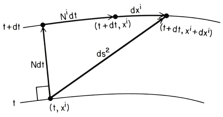
Figure 11: The $3+1$ decomposition of a spacetime metric. The figure shows two nearby members of a family of spacelike surfaces that foliate spacetime. The surfaces are labeled by a continuous coordinate $t$; points in the surfaces are labeled by three coordinates, $x^{i}$. The $3+1$ decomposition of a spacetime metric with respect to these coordinates is achieved as follows: Connect the two surfaces by a perpendicular line passing through the point $(t,x^{k})$. The lapse function $N(t,x^{k})$ is defined so that the perpendicular distance between the two surfaces separated by a coordinate interval $dt$ is $Ndt$. The shift vector $N^{i}(t,x^{k})$ is defined so that $N^{i}dt$ is the displacement between the intersection of the perpendicular with the surface $t+dt$ and the point in that surface with the same spatial coordinate $x^{i}$ as the point from which the construction started. The distance between the points $(t,x^{i})$ and $(t+dt,x^{i}+dx^{i})$ is then given by (206)

To make this distinction concrete recall the familiar $3+1$ decomposition of a four-dimensional metric defined by a foliating family of spacelike surfaces labeled by a coordinate $t$. This is illustrated in Figure 11. We write

$$ds^{2}=-N^{2}\,dt^{2}+h_{ij}\bigl{(}dx^{i}+N^{i}\,dt\bigr{)}\bigl{(}dx^{j}+N^{j}\,dt\bigr{)}$$ (206)

where the lapse $N$, shift vector $N^{i}$, and spatial metric, $h_{ij}$, are all functions of $x^{i}$ and $t$. There is a correspondence between diffeomorphisms (maps of the manifold into itself) and coordinate transformations

$$x^{\alpha}\longrightarrow\bar{x}^{\alpha}=\bar{x}^{\alpha}(x^{\beta})\,.$$ (207)

In a $3+1$ decomposition, the coordinate transformations (207) contain two special cases of interest. First, there are reparametrizations of the time

$$t\longrightarrow\bar{t}=\bar{t}(t)\,.$$ (208)

Second, there are spatial coordinate transformations

$$x^{i}\longrightarrow\bar{x}^{i}=\bar{x}^{i}(x^{j})\,.$$ (209)

Under an infinitesimal coordinate transformation of type (209), where $\bar{x}^{i}=x^{i}+\xi^{i}(x^{j})$, the three-metric transforms as

$$h_{ij}(x^{k},t)\longrightarrow\bar{h}_{ij}(x^{k},t)=h_{ij}(x^{k},t)+2D_{(i}\xi_{j)}(x^{k},t)$$ (210)

where $D_{i}$ is the spatial derivative. Because of the similarity of (210) with the symmetry transformations of gauge field theories, spatial diffeomorphisms are often called (spatial) gauge transformations.

Reparametrizations of the time and gauge transformations are combined in the invariance group of dynamical theories of spacetime geometry. However, from the point of view of the problem of time, these two types of transformation have a considerably different status. It is, therefore, convenient to consider models in which they are exhibited separately. We shall consider the simplest two model theories: free electromagnetism as an example with gauge symmetry and the free relativistic particle as an example that is reparametrization invariant. We begin with electromagnetism.

VI.2 Coarse Grainings of the Electromagnetic Field

The fine-grained histories of the free electromagnetic field we take to be specified by the various four-dimensional configurations of the potential $A^{\mu}(x)$. The allowed coarse grainings are partitions of the potentials into exhaustive sets of exclusive gauge-invariant classes, that is, classes invariant under gauge transformations

$$A_{\mu}(x)\longrightarrow A_{\mu}(x)+\nabla_{\mu}\Lambda(x)$$ (211)

for arbitrary functions $\Lambda(x)$. We denote sets of such classes by $\{c_{\alpha}\}$, $\alpha=1,2,\cdots$ and the entire class by $u=\cup_{\alpha}c_{\alpha}$. A unique potential representing a class may be singled out by imposing a gauge condition

$$\Phi(A)=0\,.$$ (212)

For example, the temporal gauge in which

$$A_{0}(x)=0$$ (213)

is often convenient. This condition does not fix the gauge entirely because transformations of the form (211) with $\Lambda$ independent of time preserve the condition (213). To fix the gauge completely a further condition, say

$$\bigl{(}\vec{\nabla}\cdot\vec{A}\bigr{)}_{\sigma}=0$$ (214)

could be imposed on one spacelike surface $\sigma$. Both (213) and (214) are included in $\Phi(A)=0$.

We can now proceed with the definition of the decoherence functional for a set of coarse-grained histories $\{c_{\alpha}\}$ that are a gauge-invariant partition of the potentials $A_{\mu}(x)$ defined on the region of spacetime between two non-intersecting spacelike surfaces $\sigma^{\prime}$ and $\sigma^{\prime\prime}$. These spacelike surfaces do not have to be planes, but for simplicity, let us consider only the case where the initial surface $\sigma^{\prime}$ is the plane $t=0$ and the final surface $\sigma^{\prime\prime}$ is the plane $t=T$ in some Lorentz frame. In that same frame there is a $3+1$ decomposition of $A_{\mu}(x)$ into the temporal component $A_{0}(x)$ and the transverse and longitudinal components of the vector potential

$$\vec{A}(x)=\vec{A}^{T}(x)+\vec{A}^{L}(x)\,,$$ (215a)

where

$$\vec{A}^{L}(x)\cdot\vec{A}^{T}(x)=0\,,\ \vec{\nabla}\cdot\vec{A}^{T}(x)=0\,.$$ (215b)

The Hilbert space of states of the free electromagnetic field is the space of square integrable functionals of transverse vector potentials, ${\cal H}^{T}$. This is defined by the inner product

$$(\psi,\chi)=\int\delta\vec{A}^{T}\psi^{*}\bigl{[}\vec{A}^{T}\bigr{]}\chi\bigl{[}\vec{A}^{T}\bigr{]}\,.$$ (216)

Here, $\psi$ and $\chi$ are functionals of $\vec{A}^{T}({\bf x})$ where ${\bf x}$ denotes the three spatial coordinates. The measure is defined by

$$\delta\vec{A}^{T}=\prod\limits_{\bf k}\,\left(dA^{1}\bigl{(}{\bf k}\bigr{)}\,d\,A^{2}\bigl{(}{\bf k}\bigr{)}\right)$$ (217)

where $A^{1}$ and $A^{2}$ are the two transverse components (polarizations) of a decomposition of $\vec{A}^{T}(\bf x)$ into modes

$$\vec{A}^{T}\left(\bf x\right)=\int\,\frac{d^{3}k}{(2\pi)^{3}}\,e^{i\bf k\cdot{\bf x}}\vec{A}^{T}\bigl{(}\bf k\bigr{)}\,.$$ (218)

Class operators $C_{\alpha}$ on ${\cal H}^{T}$ that correspond to the individual classes $c_{\alpha}$ in a gauge-invariant partition are defined by constructing their matrix elements

$$\bigl{\langle}\vec{A}^{T\prime\prime}\bigl{|}C_{\alpha}\bigr{|}\vec{A}^{T\prime}\bigr{\rangle}=\bigl{\langle}\vec{A}^{T{\prime\prime}}\bigl{|}\,\int_{\alpha}\delta A\Delta_{\Phi}[A]\,\delta[\Phi(A)]\,\exp\,\left(iS[A]\right)\,\bigr{|}\vec{A}^{T\prime}\bigr{\rangle}\,.$$ (219)

The meaning of the right hand side is as follows: The functional integral is over all potentials $A^{\mu}(x)$ that lie in the class $c_{\alpha}$ and that match the transverse component of the vector potential $\vec{A}^{T\prime}$ on the initial surface at $t=0$ and similarly match $\vec{A}^{T{\prime\prime}}$ on the final surface at $t=T$. That which is not fixed is integrated over, so the integral includes integrations over $A^{0}$ and $\vec{A}^{L}$ on the initial and final surface. The gauge-fixing $\delta$-function and its associated Faddeev-Popov determinant, $\Delta_{\Phi}$, ensure that only one representative potential in the gauge invariant class $c_{\alpha}$ contributes to the functional integral. The action for the free electromagnetic field is

$$S[A]=-\frac{1}{4}\,\int_{M}d^{4}xF_{\alpha\beta}F^{\alpha\beta}$$ (220)

where $F_{\alpha\beta}=\nabla_{\alpha}A_{\beta}-\nabla_{\beta}A_{\alpha}$ and $M$ is the spacetime region between $t=0$ and $t=T$. The measure in a time slicing implementation of the functional integral is analogous to that of Section V.2, namely

$$\delta A=\prod\limits_{t,{\bf k}}\left[dA^{1}(t,{\bf k})\,dA^{2}(t,{\bf k})\,dA^{L}(t,{\bf k})\,dA^{0}(t,{\bf k})\right]$$ (221)

in what, it is hoped, is an obvious notation. Since $\vec{A}^{T}$ is a gauge invariant quantity and since the class $c_{\alpha}$ is gauge invariant, it is a standard result Fad69 that the integral in (219) is independent of the gauge fixing condition $\Phi$. Matrix elements of the $C_{\alpha}$ between arbitrary initial and final states in ${\cal H}^{T}$ represented by wave functions $\phi_{i}[\vec{A}^{T}]$ and $\psi_{j}[\vec{A}^{T}]$ may be constructed from (219) using the inner product (216), viz. :

$$\left\langle\phi_{i}|C_{\alpha}|\psi_{j}\right\rangle=\int\delta\vec{A}^{T\prime\prime}\int\delta\vec{A}^{T\prime}\phi^{*}_{i}[\vec{A}^{T\prime\prime}]\ \langle\vec{A}^{T\prime\prime}|C_{\alpha}|\vec{A}^{T\prime}\rangle\,\psi_{j}\,[\vec{A}^{T\prime}]\,.$$ (222)

Were we to define the functional integral in (219) by means of a product formula for each mode we would be dealing with a larger Hilbert space than ${\cal H}^{T}$. This is most clearly illustrated in the temporal gauge defined by (213) and (214). Choosing the initial surface at $t=0$ to be the surface $\sigma$ on which the surface gauge condition (214) is enforced, we have

$$\langle\vec{A}^{T^{\prime\prime}}\left|C_{\alpha}\right|\vec{A}^{T^{\prime}}\rangle=\int\,\delta\vec{A}^{L^{\prime\prime}}\langle\vec{A}^{T^{\prime\prime}}\ ,\vec{A}^{L^{\prime\prime}}\|\,\int_{\alpha}\delta\vec{A}\exp\,(iS[\vec{A}])\|\,\vec{A}^{T^{\prime}}\,,0\rangle\,.$$ (223)

Here, we have used a double bar to denote states in the Hilbert space ${\cal H}^{(T,L)}$ of square integrable functionals of vector potentials — both transverse and longitudinal components. The functional integral in (223) is over such vector potentials. There is an integral over the final value of $\vec{A}^{L^{\prime\prime}}$ but the initial value has been set to zero by the surface gauge condition (214). The auxiliary Hilbert spaces ${\cal H}^{L}$ and ${\cal H}^{(T,L)}$ will be useful in evaluating functional integrals in what follows and in making contact with Dirac Quantization in Section VI.5.

Having identified the class operators $C_{\alpha}$, the construction of the decoherence functional $D(\alpha^{\prime},\alpha)$ for the coarse-grained set of histories $\{c_{\alpha}\}$ follows that for particle quantum mechanics [cf. (150)]:

$$D\left(\alpha^{\prime},\alpha\right)={\cal N}Tr\bigl{[}\rho_{f}C_{\alpha^{\prime}}\,\rho_{i}\,C^{\dagger}_{\alpha}\bigr{]}$$ (224a)

where $${\cal N}$$ is

$${\cal N}^{-1}=Tr\left[\rho_{f}e^{-iH^{T}T}\rho_{i}e^{iH^{T}T}\right]\,.$$ (224b)

Here, $\rho_{i}$ and $\rho_{f}$ are density matrices describing the initial and final conditions of the electromagnetic system. These $\rho$’s, the $C_{\alpha}$, and the trace are all defined on the Hilbert space, ${\cal H}^{T}$. If we assume a final condition of indifference with respect to final state we recover the standard

$$D\left(\alpha^{\prime},\alpha\right)=Tr[C_{\alpha^{\prime}}\rho_{i}C^{\dagger}_{\alpha}]\,.$$ (225)

Thus, the two gauge-invariant parts of the vector potential, $\vec{A}^{T}({\bf x})$ and $\vec{A}^{L}({\bf x})$, are treated differently in the construction of the decoherence functional. Amplitudes, e.g. (223) are summed over $\vec{A}^{L}({\bf x})$ on the final surface; squares of amplitudes are summed over $\vec{A}^{L}({\bf x})$ in (224). For suitable coarse grainings this coincides with usual Hamiltonian quantum mechanics as we shall shortly see.

It is not difficult to check that the decoherence functional (224) satisfies the requirements (117a) – (117d) of Section IV. Hermiticity and positivity are immediate from the general structure of (224) and the positivity of the $\rho$’s. The superposition principle is satisfied because of the linearity of the sum-over-histories in (219). It only remains to check the normalization, and this involves the sum in (223) over all vector potentials $\vec{A}(x)$. This factors into separate sums over $\vec{A}^{T}$ and $\vec{A}^{L}$ involving the temporal gauge actions

$$S\bigl{[}\vec{A}^{T}\bigr{]} = {\textstyle{1\over 2}}\,\int\,d^{4}x\,\biggl{[}\Bigl{(}{\buildrel\textstyle{\buildrel\textstyle.\over{\rightarrow}}\over{A^{T}}}\Bigr{)}^{2}-\left(\vec{\nabla}\times\vec{A}^{T}\right)^{2}\biggr{]}\,,$$ (226a)

$$S\bigl{[}\vec{A}^{L}\bigr{]} = {\textstyle{1\over 2}}\,\int\,d^{4}x\Bigl{(}{\buildrel\textstyle{\buildrel\textstyle.\over{\rightarrow}}\over{A^{L}}}\Bigr{)}^{2}\,.$$ (226b)

Then, from the usual connection to Hamiltonian quantum mechanics

$$\bigl{\langle}\vec{A}^{T^{\prime\prime}}\left|C_{u}\right|\vec{A}^{T^{\prime}}\bigr{\rangle}=\bigl{\langle}\vec{A}^{T^{\prime\prime}}\bigl{|}e^{-iH^{T}T}\bigr{|}\vec{A}^{T^{\prime}}\bigr{\rangle}\,\int\,\delta\vec{A}^{L^{\prime\prime}}\bigl{\langle}\vec{A}^{L^{\prime\prime}}\bigl{|}e^{-iH^{L}T}\bigr{|}\vec{A}^{L^{\prime}}=0\bigr{\rangle}\,.$$ (227)

In this expression where we have used a single bar to denote the inner product in either ${\cal H}^{T}$ or ${\cal H}^{L}$ and $H^{T}$ and $H^{L}$ are the Hamiltonians corresponding to the actions (226), specifically:

$$H^{T} = {\textstyle{1\over 2}}\,\int\,d^{3}x\,\bigl{[}(\vec{\pi}^{T})^{2}+(\vec{\nabla}\times\vec{A}^{T})^{2}\bigr{]}\,,$$ (228a)

$$H^{L} = {\textstyle{1\over 2}}\,\int\,d^{3}x\,(\vec{\pi}^{L})^{2}\,.$$ (228b)

The last factor in (227), including the integral, can be written

$$\left\{\int\,\delta\vec{A}^{L^{\prime\prime}}\exp\,\left[-i\,\int\,d^{3}x\bigl{(}\vec{\pi}^{L^{\prime\prime}}\cdot\vec{A}^{L^{\prime\prime}}\bigr{)}\right]\bigl{\langle}\vec{A}^{L^{\prime\prime}}\bigl{|}\,e^{-iH^{L}T}\bigr{|}\vec{A}^{L^{\prime}}=0\bigr{\rangle}\right\}_{\vec{\pi}_{L}=0}$$

$$=\bigl{\langle}\vec{\pi}^{L^{\prime\prime}}=0\bigl{|}\,e^{-iH^{L}T}\bigr{|}\vec{A}^{L^{\prime}}=0\bigr{\rangle}\,\big{/}\,\bigl{\langle}\vec{\pi}^{L^{\prime\prime}}=0\big{|}\vec{A}^{L^{\prime}}=0\bigr{\rangle}\,.$$ (229)

But, since $H^{L}$ conserves $\vec{\pi}^{L}$, the factor (227) is just unity. Thus,

$$C_{u}=e^{-iH^{T}T}\,,$$ (230)

and the normalization of the decoherence functional (224) follows immediately.

VI.3 Specific Examples

Specific types of coarse grainings are of interest. First, consider partitions by ranges of values of $\vec{A}^{T}({\bf x})$ on a surface of constant time $t$ between $0$ and $T$. These are the usual gauge-invariant, configuration-space observables of electromagnetism. From the explicit forms (223) and (227) and a repetition of the discussion in Section III.1.4, it follows that

$$C_{\alpha}=e^{-iH^{T}(T-t)}P_{\alpha}e^{-iH^{T}t}$$ (231)

where the $P_{\alpha}$ are projections in ${\cal H}^{T}$ onto the ranges of $\vec{A}^{T}({\bf x})$. Similarly, for coarse grainings defined by sequences of sets of alternative ranges of $\vec{A}^{T}({\bf x})$, at times $t_{1},\cdots,t_{n}$, one has

$$C_{\alpha}=e^{-iH^{T}(T-t_{n})}P^{n}_{\alpha_{n}}e^{-iH^{T}(t_{n}-t_{n-1})}P^{n-1}_{\alpha_{n-1}}\cdots P^{1}_{\alpha_{1}}e^{-iH^{T}t_{1}}\ .$$ (232)

In these expressions one recovers the familiar Hamiltonian quantum mechanics of the “true degrees of freedom” of the electromagnetic field. These true degrees of freedom are the transverse components of the vector potential. As in Section III.1, the quantum theory can be formulated in terms of states represented by wave functionals $\psi[\vec{A}^{T},t)$ that evolve unitarily in between projections defining specific alternatives. When restricted to coarse grainings of the true physical degrees of freedom on spacelike surfaces this sum-over-histories quantum mechanics coincides with the usual Hamiltonian quantum mechanics of the free electromagnetic field.

However, more general kinds of coarse-graining that are defined by alternatives not at one moment of time are also possible. For example, one can partition the potentials $A^{\mu}(x)$ by ranges of values of particular field components averaged over a spacetime region that were considered by Bohr and Rosenfeld BR33 in their discussion of the measurability of the electromagnetic field. These are partitions by the values of functionals of the potential of the form

$$F[A]=\frac{1}{V(R)}\,\int_{R}d^{4}x\,F_{\mu\nu}(x)\,.$$ (233)

where $V(R)$ is the volume of spacetime region $R$. (We tolerate, just briefly, the use of $F$ for both field and functional.) Partitions by values of averages of the magnetic field, say

$$F_{B_{z}}[A]=\frac{1}{V(R)}\,\int_{R}d^{4}x\,B_{z}(x)=\frac{1}{V(R)}\,\int_{R}d^{4}x\left(\vec{\nabla}\times\vec{A}^{T}\right)_{z}$$ (234)

are describable entirely in terms of the “true physical degrees of freedom” of the electromagnetic field. Their class operators may be computed on ${\cal H}^{T}$ by the techniques described in Section V. Indeed, since the free electromagnetic field is equivalent to an assembly of oscillators we expect these class operators to be computable explicitly. As in the case of spacetime alternatives for the non-relativistic particle, we do not recover an alternative formulation of the generalized quantum mechanics of these alternatives in terms of evolving states on a spacelike surface reduced by the action of projections.

We cannot coarse grain by values of $\vec{A}^{L}$ at a moment of time because $\vec{A}^{L}$ is not gauge-invariant. We can, however coarse grain by ranges of values of the electric field that involve $\vec{A}^{L}$, for example, the following field average:

$$F_{E_{z}}[A]=\frac{1}{V(R)}\,\int_{R}d^{4}x\,E_{z}(x)=\frac{1}{V(R)}\,\int_{R}d^{4}x\bigl{(}\vec{\nabla}A_{0}-{\buildrel\textstyle{\buildrel\textstyle.\over{\rightarrow}}\over{A}}\bigr{)}_{z}\,.$$ (235)

Such coarse grainings are gauge-invariant, calculable by the techniques in Section V, but not directly expressible in terms of the “true physical degrees of freedom” alone. In the limit as the temporal size of $R$ goes to zero such coarse grainings will be vacuous as were the coarse grainings by $\dot{q}$ in Section V. In the limit as the temporal size of $R$ becomes large, however, such coarse grainings coincide with coarse grainings by canonical field momenta as we shall see next.

VI.4 Constraints

Classically, the gauge invariance of electromagnetism implies a constraint between its canonical coordinates $\vec{A}({\bf x})$ and the corresponding canonical momenta $\vec{\pi}({\bf x})$. The canonical momenta are found from the Lagrangian density of the action (220):

$$\vec{\pi}(x)=\frac{\partial{\cal L}}{\partial{\buildrel\textstyle{\buildrel\textstyle.\over{\rightarrow}}\over{A}}(x)}=-\vec{E}(x)={\buildrel\textstyle{\buildrel\textstyle.\over{\rightarrow}}\over{A}}(x)-\vec{\nabla}A_{0}(x)\,.$$ (236)

The constraint is the field equation

$$\vec{\nabla}\cdot\vec{E}({\bf x})=0\,,$$ (237)

or, what is the same thing,

$$\vec{\pi}^{L}({\bf x})=0\,.$$ (238)

Physical states are annihilated by operator forms of the classical constraints in the Dirac approach to quantization. To what extent are the constraints maintained in the present sum-over-histories quantization of electrodynamics?

Whether a relation like (237) is satisfied in quantum theory is not a question of definition, but a matter of probability. The divergence of the electric field is a measurable quantity and a theory that does not assign probabilities to its possible values is incomplete. This theory assigns probabilities to alternative values of $\vec{\nabla}\cdot\vec{E}$ if they decohere. The constraints can be said to be satisfied if the probability vanishes for every value of $\vec{\nabla}\cdot\vec{E}$ except zero. We shall now compute the probabilities for various values of the longitudinal component of the field momentum, $\vec{\pi}^{L}({\bf x})$

Momentum is accessible in a sum-over-histories formulation of quantum field theory in essentially the same way that we discussed for a sum-over-histories formulation of quantum particle mechanics in Section V.4 . Coarse grainings by average values of time derivatives of fields become partitions by field momentum when the time over which the average is taken becomes large. We, therefore, consider partitions by values of the gauge invariant functional:

$$\vec{F}_{\bf x}[A]=\frac{1}{\Delta t}\,\int^{t_{2}}_{t_{1}}dt\,\vec{\pi}^{L}({\bf x},t)=\frac{1}{\Delta t}\,\int^{t_{2}}_{t_{1}}dt\,\Bigl{[}{\buildrel\textstyle{\buildrel\textstyle.\over{\rightarrow}}\over{A^{L}}}\left({\bf x},t\right)-\vec{\nabla}A_{0}\left({\bf x},t\right)\Bigr{]}\,.$$ (239)

where $0<t_{1}<t_{2}<T$ and $\Delta t=t_{2}-t_{1}$. In the limit that $\Delta t$ becomes large, this becomes a partition by $\vec{\pi}^{L}({\bf x})$. This is especially transparent in the temporal gauge where the analogy with particle momenta is immediate. As we shall show in more detail below, if we follow the analysis of Section V.4, in the limit of large $\Delta t$ the sum over $A^{\mu}(x)$ in the class with a particular range of values $\widetilde{\Delta}$ of the average (239) can be replaced by a projection, $P_{\tilde{\Delta}}$, onto the range of eigenvalues of the operator:

$$\vec{\pi}^{L}({\bf x})=-i\delta/\delta\vec{A}^{L}({\bf x})\,.$$ (240)

Further, the class operators for alternative ranges of $\vec{\pi}^{L}(\bf x)$ will be shown to vanish except for ranges which include $\vec{\pi}^{L}({\bf x})=0$, essentially as a consequence of the gauge invariance of the construction of the decoherence functional. A vanishing probability is thus predicted for every value of $\vec{\pi}^{L}({\bf x})$ except zero, and it is in this sense that the constraint is satisfied.

For simplicity let us consider a partition by the time average of just a single mode of the scalar $\pi^{L}$, specifically by the functional $F_{\bf k}[A]$ which in the temporal gauge is [cf. (198)]:

$$F_{\bf k}[A]=\frac{1}{\Delta t}\left[A^{L}({\bf k},t_{2})-A^{L}({\bf k},t_{1})\right]\,.$$ (241)

The matrix elements of the class operator corresponding to $F_{\bf k}[A]$ lying in the range $\tilde{\Delta}$ are

$$\bigl{\langle}\vec{A}^{T\prime\prime}|C_{\tilde{\Delta}}|\vec{A}^{T\prime}\bigr{\rangle}=\langle\vec{A}^{T\prime\prime}|\int\nolimits\delta A\Delta_{\Phi}[A]\delta[\Phi(A)]e_{\tilde{\Delta}}(F_{\bf k}[A])\exp(iS[A])|\vec{A}^{T\prime}\rangle$$ (242)

where $e_{\tilde{\Delta}}(x)$ is the characteristic function for the interval $\tilde{\Delta}$. The integral over the transverse parts of $\vec{A}$ is unrestricted by the coarse graining as are the integrals over longitudinal modes except those with wave-vector ${\bf k}$. The class operator matrix elements may therefore be written

$$\langle\vec{A}^{T\prime\prime}|C_{\tilde{\Delta}}|\vec{A}^{T\prime}\rangle=\langle\vec{A}^{T\prime\prime}|e^{-iH^{T}T}|\vec{A}^{T\prime}\rangle{\cal C}_{\tilde{\Delta}}$$ (243)

where

$${\cal C}_{\tilde{\Delta}}=\int_{\tilde{\Delta}}df\,{\cal C}_{f}$$ (244)

and ${\cal C}_{f}$ is the functional integral over the mode $A^{L}({\bf k},t)$ restricted to those histories where $F_{\bf{k}}[A]$ has the value $f$. Specifically,

$${\cal C}_{f}=\int\nolimits dA^{L\prime\prime}\int\nolimits dA^{L}_{2}\int\nolimits dA^{L}_{1}\,\delta\left[(A^{L}_{2}-A^{L}_{1})/{\Delta t}-f\right]$$

$$\langle A^{L\prime\prime},T|A^{L}_{2},t_{2}\rangle\,\langle A^{L}_{2},t_{2}|A^{L}_{1},t_{1}\rangle\,\langle A^{L}_{1},t_{1}|A^{L\prime}=0,0\rangle\,.$$ (245)

In this expression $\langle A^{L\prime\prime},t^{\prime\prime}|A^{L\prime},t^{\prime}\rangle$ is the propagator of the longitudinal part of the vector potential constructed with the Hamiltonian $H^{L}$. We have suppressed all the labels ${\bf k}$ that refer to the particular mode summed over. We have used the surface gauge condition (214) to fix the initial integration. The final integration turns the final propagator in the series of three into $\langle\pi^{L\prime\prime}=0,T|A^{L}_{2},t_{2}\rangle$ which is unity. With the Hamiltonian (228b) the remaining propagator in (245) is just that of a free particle. Using the $\delta$-function to carry out the integral over $A^{L}_{2}$ and making use of the invariance of this propagator under translations both in time and $A^{L}$, we find that

$${\cal C}_{f}=\Delta t\langle f\Delta t,\Delta t|0,0\rangle\,,$$ (246)

and more explicitly

$${\cal C}_{\tilde{\Delta}}=\left(\frac{\Delta t}{2\pi i}\right)^{\textstyle{1\over 2}}\int_{\tilde{\Delta}}\,dfe^{i(\Delta tf^{2})/2}\,.$$ (247)

In the limit $\Delta t\to\infty$, ${\cal C}_{\widetilde{\Delta}}$ vanishes unless $\widetilde{\Delta}$ contains $f=0$. In this limit the partition defines momentum $\pi^{L}({\bf k})$ and this result is a more detailed demonstration that the class operators vanish except when $\pi^{L}({\bf k})=0$. If we consider a partition of the real line by intervals $\{\Delta_{\alpha}\},\alpha=1,2,\cdots$, then the decoherence functional is

$$D(\alpha^{\prime},\alpha)={\cal C}_{\tilde{\Delta}_{\alpha^{\prime}}}{\cal C}_{\tilde{\Delta}_{\alpha}}.$$ (248)

Since the ${\cal C}$ ’s are non-zero only for a single $\alpha$, this coarse-grained set of alternatives decoheres and the probability is zero for any value of $\alpha$ except that corresponding to the interval containing $\pi^{L}({\bf k})=0$. If $\hbar$ is restored by replacing $t$ with $t/\hbar$, then the same result is obtained for any $\Delta t$ in the formal “classical limit” $\hbar\to 0$. It is in these precise probabilistic senses that the constraint is satisfied in this generalized quantum mechanics of the electromagnetic field. Thus, restricting the initial and final conditions to depend only on the “true physical degrees of freedom”, $\vec{A}^{T}$, means that $\vec{\pi}^{L}=0$ with probability one at all other times. This is a familiar result in the more usual quantum mechanics of states on spacelike surfaces as we shall discuss below.

If $\hbar$ and $\Delta t$ are finite then the ${\cal C}$’s will be non-zero for several different values of $\alpha$. Such alternatives cannot decohere. The decoherence functional (248) factors and the off-diagonal elements cannot vanish without the diagonal ones vanishing also. Probabilities are therefore not assigned to such alternatives in the theory of the free electromagnetic field.

VI.5 ADM and Dirac Quantization

The relation of the present generalized quantum mechanics of the electromagnetic field with Arnowitt-Deser-Misner (ADM) and Dirac quantization is of interest. In ADM quantization the constraints are solved classically. Thus, $\vec{\nabla}\cdot\vec{E}=0$ once and for all. Now, certainly $\vec{\nabla}\cdot\vec{E}$ is a measurable quantity although in the ADM approach it does not correspond to an operator in Hilbert space. However, as we mentioned earlier, any quantum theory of the electromagnetic field must predict a probability for $\vec{\nabla}\cdot\vec{E}$ since we can observe it even on “macroscopic” scales. The quantum theory would be incomplete if it did not offer such a prediction. Presumably, ADM theory predicts that a measurement of $\vec{\nabla}\cdot\vec{E}$ at a moment of time would yield its classical value zero with probability one. One also presumes that ADM quantization would predict zero probability for all but zero values of the time average of $\vec{\nabla}\cdot\vec{E}$ represented by (239). If so, then it differs in its predictions from the present discussion where the class operators given by (242) and (247) do not vanish for values of these time averages of $\vec{\nabla}\cdot\vec{E}$ other than zero. The question of agreement is perhaps moot in the case of free electromagnetism because alternatives defined by sets of ranges of averages of $\vec{\nabla}\cdot\vec{E}$ over finite times do not decohere and probabilities are not, therefore, predicted for them. However, in the presence of charges such alternatives might decohere and then the predictions of the generalized quantum mechanics would differ from ADM theory naively interpreted. In assessing these contrasts, it should be kept in mind that they concern predictions gauge-invariant quantities which, although observable, are not constructed from the “true physical degrees of freedom”. Further, the differences arise for alternatives extended over time that are not usually considered in quantum mechanics. A generalization of quantum which includes such quantities is perhaps going beyond the domain of questions that ADM theory was intended to answer.

Dirac quantization is another familiar approach to the quantum mechanics of constrained Hamiltonian systems such as the free electromagnetic field. Dirac quantization employs an extended linear space, ${\cal L}^{(T,L)}$, of functionals of the vector potential, $\vec{A}({\bf x})$. Observables commute with operator representations of the constraints and physical states are represented by functionals that are annihilated by them. The linear space ${\cal L}^{(T,L)}$ cannot be the Hilbert space ${\cal H}^{(T,L)}$ because solutions of the constraint $\pi^{L}\psi=0$ are functionals of $\vec{A}^{T}$ alone and are therefore not square integrable. For the electromagnetic field Dirac and ADM quantization are fully equivalent as usually interpreted Kuc86 . If that is true, Dirac quantization would share with ADM the differences with the present approach for the predictions values of gauge-invariant quantities that are not “time degrees of freedom” when extended over time. Despite this difference we can still ask whether we can construct anything like the operators and states of Dirac quantization in the present approach. The following are possible:

Class operators corresponding to a set of coarse-grained histories $\{c_{\alpha}\}$ may be introduced on ${\cal H}^{(T,L)}$ by specifying their matrix elements by

$$\bigl{\langle}\vec{A}^{\prime\prime}\|\,C_{\alpha}\|\vec{A}^{\prime}\bigr{\rangle}=\bigl{\langle}\vec{A}^{\prime\prime}\|\,\int_{\alpha}\delta A\,\Delta_{\tilde{\Phi}}[A]\,\delta\,\bigl{[}\tilde{\Phi}(A)\bigr{]}\,\exp\,\left(iS[A]\right)\|\vec{A}^{\prime}\bigr{\rangle}\ .$$ (249)

The functional integral is over the potentials $A^{\mu}(x)$ that lie in the class $c_{\alpha}$ and match the prescribed vector potentials on the initial and final surfaces. $\tilde{\Phi}$ is a gauge fixing condition that does not include a surface gauge fixing condition as in (214) since the corresponding gauge freedom is already fixed by the specification of the vector potentials on the initial and final surfaces. Indeed, $\tilde{\Phi}$ must be such as to not restrict $\vec{A}({\bf x})$ on the initial and final surfaces at all.

The operators so defined are independent of $\tilde{\Phi}$ in the class of $\tilde{\Phi}$ generated from a given one by gauge transformations that preserve the initial and final vector potentials. That is, they depend only on the class of gauge fixing conditions of the form $\tilde{\Phi}^{\Lambda}(A)=\tilde{\Phi}(A+\nabla\Lambda)$ for some fixed $\tilde{\Phi}$ as $\Lambda$ ranges over such gauge transformations.

The class operators on ${\cal H}^{(T,L)}$ exhibited in (223) could be used as the starting point for the construction of the decoherence functional (224). However, to incorporate initial and final conditions represented by wave functions $\phi_{i}[\vec{A}^{T}]$ and $\psi_{j}[\vec{A}^{T}]$ that are solutions of the constraints we cannot use the inner product on ${\cal H}^{(T,L)}$ because such wave functions do not lie in that space. Rather we must attach initial and final wave functions as in (222)

$$\left\langle\phi_{i}|C_{\alpha}|\psi_{j}\right\rangle=\int d\vec{A}^{T\prime\prime}\int d\vec{A}^{T\prime}\int d\vec{A}^{L\prime\prime}\phi^{*}_{i}[\vec{A}^{T\prime\prime}]\,\langle\vec{A}^{T\prime},\vec{A}^{L\prime\prime}\|C_{\alpha}\|\vec{A}^{T\prime},0\rangle\,\psi_{j}[\vec{A}^{T\prime}]\,.$$ (250)

essentially making use of the inner product on ${\cal H}^{T}$. The decoherence functional could then be constructed as in (150) and is equivalent to (224). Such constructions involving separate linear spaces for functional integrals and initial and final conditions will be essential in defining the generalized quantum mechanics of reparametrization invariant systems.

Although the generalized quantum mechanics under discussion does usually permit a notion of state on a spacelike surface, the above construction suggests a way of associating a branch wave functional on ${\cal L}^{(T,L)}$ with each branch of an initial pure state $|\psi\rangle$ corresponding to a coarse-grained history $c_{\alpha}$. Define the extended wave functional by

$$\Psi_{\alpha}\bigl{[}\vec{A}^{\prime\prime}\bigr{]}=\int\,\delta\vec{A}^{\prime}\bigl{\langle}\vec{A}^{\prime\prime}\left\|\,C_{\alpha}\right\|\vec{A}^{\prime}\bigr{\rangle}\psi\bigl{[}A^{T\prime}\bigr{]}\,.$$ (251)

This branch wave functional is independent of the gauge fixing condition in the class generated from a given one by gauge transformations that leave $\vec{A}^{\prime\prime}({\bf x})$ unchanged.

The branch wave functions $\Psi_{\alpha}[\vec{A}]$ may be thought of as “states of the system” on the final spacelike surface $t=T$. Indeed, if we limit attention to coarse grainings that restrict the values of $\vec{A}$ only on a family of spacelike surfaces labeled by $t$, then is it is possible to define states on these surfaces represented by wave functions $\Psi_{\beta}[\vec{A},t]$ by following the construction described in Section IV.4. These states would have the form of (251) but with the functional integrals defining $\langle\vec{A}^{\prime\prime}\|C_{\beta}\|\vec{A}^{\prime}\rangle$ limited to times less than $t$ and restricted only by the coarse graining there.

We are now in a position to ask whether the extended class operators defined by (249) commute with the constraint and whether the wave functional of the individual branches are annihilated by it. The simplest example of a gauge condition that does not restrict the vector potentials on either the initial or final surfaces is the temporal gauge. In this gauge, the question of commutation is easily analyzed directly. Shift the variable of integration in (249) by the gauge transformation

$$\vec{A}\left(t,{\bf x}\right)\longrightarrow\vec{A}\left(t,{\bf x}\right)+\vec{\nabla}\epsilon\left({\bf x}\right)$$ (252)

where $\epsilon({\bf x})$ is independent of time. Of course, the integral is not changed by this shift in integration variable. But also, because this shift is a gauge transformation, the action and measure are left unchanged. Because it is a time-independent gauge transformation the temporal gauge is preserved. Thus, (249) is unchanged when the initial and final $\vec{A}(\bf x)$ are shifted as in (252) by the same amount. Since $\vec{\pi}^{L}(\bf x)$ is the operator that effects such a shift [cf. (240)], this is equivalent to

$$\bigl{[}\vec{\pi}^{L}\left({\bf x}\right),C_{\alpha}\bigr{]}=0$$ (253)

so constraints commute with the extended class operators. It is then an immediate consequence of (253) and $\vec{\pi}^{L}({\bf x})\psi(\vec{A}^{T})=0$ that

$$\vec{\pi}^{L}({\bf x})\Psi_{\alpha}\bigl{[}\vec{A}\bigr{]}=0\,.$$ (254)

The wave functionals representing the branches of gauge invariant coarse graining thus satisfy the Dirac constraint condition. Restricting the initial and final conditions to wave functions that depend only on the “true physical degrees of freedom” means that wave functions representing states at intermediate times also depend only on these.

We have derived these results in the temporal gauge. However, both (253) and (254) are more general because the functional integrals defining $C_{\alpha}$ and $\Psi_{\alpha}$ are independent of the gauge fixing condition in the classes discussed above.

There are thus two distinct ways in which the constraints can be said to be satisfied in the generalized quantum mechanics of electromagnetism under discussion. First $\vec{\pi}^{L}({\bf x})$ is a gauge-invariant quantity which can be given meaning in a sum-over-histories formulation of quantum mechanics as average values of field “velocities” over very long times. The theory predicts probabilities for alternative values of $\vec{\pi}^{L}({\bf x})$ when these alternatives decohere. The probability is zero for values other than $\vec{\pi}^{L}({\bf x})=0$. Second, when class operators and branch wave functionals are defined on the configuration space of vector potentials as described, then the class operators commute with the constraints and the branch wave functions are annihilated by them. In these senses the generalized quantum mechanics of electromagnetism makes contact with the ideas of Dirac quantization. When restricted to gauge invariant partitions by potential or momenta at definite moments of time, the predictions of the generalized quantum mechanics described here coincide with those of the Dirac procedure. In considering gauge invariant alternatives which are extended over time, however, it goes beyond either Dirac or ADM quantization in their usual senses.

VII Models with a Single Reparametrization Invariance

VII.1 Reparametrization Invariance in General

Generalized quantum mechanical theories are specified by their fine-grained histories, their allowable coarse grainings, and their decoherence functional. In this section we shall construct examples of such theories for a class of models whose unique set of fine-grained histories are curves in a configuration space ${\cal C}$ spanned by coordinates $Q^{i},\;i=1,\cdots,\nu$. The $Q^{i}$ include the variables describing the physical time, if there is one. The most familiar example is the relativistic particle whose fine-grained histories are curves in spacetime.

Curves may be described parametrically by giving the coordinates as functions of a parameter $\lambda$, viz. $Q^{i}(\lambda)$. We shall frequently suppress the coordinate labels and write $Q$ for a point in the configuration space and $Q(\lambda)$ for a curve. The curves are the fine-grained histories, not the functions $Q^{i}(\lambda)$ that describe how the paths are parametrized. For this reason these theories are reparametrization invariant. The action summarizing dynamics and the partitions defining allowed coarse grainings may both be conveniently described in terms of the functions $Q^{i}(\lambda)$, but they both must be invariant under reparametrizations:

$$\lambda\rightarrow\bar{\lambda}=f(\lambda)\,.$$ (255)

The most natural choice for the set of fine-grained histories is often the set of all curves in ${\cal C}$ including those which cross and recross the surfaces of constant time if there is one. However, different theories can be obtained by restricting the set of fine-grained histories, for example, to curves that intersect hypersurfaces of a preferred time coordinate once and only once. We shall illustrate the effects of such choices in the models below.

As we shall see below, reparametrization invariance implies a constraint between the coordinates and their canonical momenta. The quantum mechanics of such a constrained theory is often most conveniently formulated on an extended configuration space ${\cal C}_{\rm ext}$ of coordinates $Q^{i}$ and a multiplier enforcing the constraint. The free relativistic particle provides the simplest example. The configuration space ${\cal C}$ is Minkowski spacetime and the fine-grained histories are curves $x^{\alpha}(\lambda)$ in this spacetime. A classical action for the relativistic particle is the spacetime interval along its curve

$$S[x^{\alpha}]=m\int d\tau\equiv m\int^{1}_{0}d\lambda\left[-\eta_{\alpha\beta}\left(\frac{dx^{\alpha}}{d\lambda}\right)\left(\frac{dx^{\beta}}{d\lambda}\right)\right]^{\textstyle{1\over 2}}$$ (256)

where $m$ is the particle’s rest mass, $\eta_{\alpha\beta}$ is the Minkowski metric and we have arbitrarily chosen $0$ and $1$ as the values of the parameter labeling the ends of the curve. (In previous sections we have used $\tau$ for a dummy argument variable. In this section it means proper time.) The action (256) is manifestly reparametrization invariant and its extrema satisfy the correct relativistic equations of motion. However, it is not the only classical action with these properties. Different actions with the same extrema are equivalent classically, but in quantum mechanics it is not just the extrema of the action which are important. The value of the action on non-extremal curves also contributes to amplitudes through path-integrals of $\exp(iS)$. Different forms of the action will therefore generally lead to different sum-over-histories quantum theories assuming that the relevant sums over $\exp(iS)$ can be defined at all.

The action (256) cannot easily be used to formulate a sum-over-histories quantum mechanics of the relativistic particle because it is not quadratic in the velocities. An action which does the job can be formulated on the extended configuration space ${\cal C}_{\rm ext}$ of paths $x^{\alpha}(\lambda)$ and multiplier $N(\lambda)$. It is

$$S\left[x^{\alpha},N\right]=\frac{m}{2}\int^{1}_{0}d\lambda N(\lambda)\left[\left(\frac{\dot{x}(\lambda)}{N(\lambda)}\right)^{2}-1\right]$$ (257)

where a dot denotes a derivative with respect to $\lambda$ and $(\dot{x})^{2}=\eta_{\alpha\beta}\dot{x}^{\alpha}\dot{x}^{\beta}$. The action (257) yields the correct equations of motion when extremized with respect to $x^{\alpha}(\lambda)$ and $N(\lambda)$ and it is invariant under the reparametrization transformations

$$x^{\alpha}(\lambda)\rightarrow\bar{x}^{\alpha}(\lambda) = x^{\alpha}\bigl{(}f(\lambda)\bigr{)}\,,$$ (258a)

$$N(\lambda)\rightarrow\bar{N}(\lambda) = N\bigl{(}f(\lambda)\bigr{)}\dot{f}(\lambda),$$ (258b)

provided $f(0)=0$ and $f(1)=1$ so the values of $x^{\alpha}$ and $\lambda$ at the ends of the history are unchanged. As we shall show in detail in Section VII.4 and VII.5, the action (257) leads to correct and manageable quantum theories of the relativistic particle. Thus generally we take for the fine-grained histories of a reparametrization-invariant theory curves $(Q(\lambda),N(\lambda))$ in ${\cal C}_{\rm ext}$.

The second element of a generalized quantum mechanics is the class of allowed coarse grainings. For a reparametrization-invariant theory, the general notion of a coarse graining is a partition of the fine-grained histories — curves in ${\cal C}_{\rm ext}$ — into exclusive reparametrization invariant classes $\{c_{\alpha}\}$. More specifically, each class must be invariant under the reparametrization transformation

$$Q^{i}(\lambda)\rightarrow\bar{Q}^{i}(\lambda) = Q^{i}\bigl{(}f(\lambda)\bigr{)}\,,$$ (259a)

$$N(\lambda)\rightarrow\bar{N}(\lambda) = N\bigl{(}f(\lambda)\bigr{)}\dot{f}(\lambda)\,,$$ (259b)

for $f(\lambda)$ that leave the parameters of the endpoints of the curve unchanged. Examples of reparametrization invariant coarse grainings are readily exhibited: Given a spacetime region $R$, the paths may partitioned into the class of paths that never cross $R$ and the class of paths that cross $R$ at least once. Given a hypersurface in configuration space the paths may be partitioned by the value of $Q$ at which they first cross the hypersurface starting from one end.

Further examples can be constructed by introducing the arc-length along a curve. The multiplier $N(\lambda)$ allows reparametrization invariant arc-length

$$\tau\bigl{(}\lambda^{\prime\prime},\lambda^{\prime},N(\lambda)\bigr{]}=\int^{\lambda^{\prime\prime}}_{\lambda^{\prime}}N(\lambda)d\lambda$$ (260)

to be defined between any two points along a curve that are defined in a reparametrization invariant manner. For instance, we might consider the arc-length $\tau$ of paths that connect two points $Q^{\prime}$ and $Q^{\prime\prime}$. The paths may then be partitioned using this additional invariant structure. For example, the paths starting from point $Q^{\prime}$ could be partitioned by the positions $Q$ they have arrived at after a given length $\tau$.

The most general notion of coarse graining is a partition by ranges of values of reparametrization invariant functionals of the paths and multiplier $F[Q(\lambda),N(\lambda)]$. All of the above examples can be characterized in this way.

A decoherence functional completes the specification of a generalized quantum mechanics. For a given coarse graining consisting of classes $\{c_{\alpha}\}$ this will be constructed from path-integrals over the classes of the form

$$\left\langle Q^{\prime\prime}\left\|C_{\alpha}\right\|Q^{\prime}\right\rangle\equiv\sum\limits_{{\rm path}\ \in[Q^{\prime}c_{\alpha}Q^{\prime\prime}]}\exp\Bigl{(}iS[{\rm path}]\Bigr{)}$$ (261)

where the sum is over all paths in ${\cal C}_{\rm ext}$ that begin at $Q^{\prime}$, end at $Q^{\prime\prime}$, and are in the class $c_{\alpha}$. To make this precise we need to specify the action, measure, and the product formula with which the sums in (261) are defined. There is a canonical way of doing this which is somewhat lengthy to describe so we shall take it up separately in Section VII.2 below. For the moment, we simply note that, in cases where the path integral is defined by a product formula, the most natural Hilbert space involved is ${\cal H}^{Q}$ — the space of square-integrable functions on the configuration space ${\cal C}$ spanned by the $Q^{i}$. The matrix elements (261) then define a class operator $C_{\alpha}$ on ${\cal H}^{Q}$. We have used a double bar to denote the inner product on ${\cal H}^{Q}$.

Following the example of non-relativistic quantum mechanics discussed in Section V, the next step in the construction of the decoherence functional is to adjoin initial and final conditions represented respectively by wave functions $\{\psi_{j}(Q)\}$ and $\{\phi_{i}(Q)\}$ and their associated probabilities. In non-relativistic quantum mechanics we did this using the same inner product that was used to define the path-integrals. However, it will prove to be important for reparametrization invariant theories to allow a more general construction. We define

$$\left\langle\phi_{i}\left|C_{\alpha}\right|\psi_{j}\right\rangle=\phi_{i}(Q^{\prime\prime})\circ\left\langle Q^{\prime\prime}\left\|C_{\alpha}\right\|Q^{\prime}\right\rangle\circ\psi_{j}(Q^{\prime})$$ (262)

where the $\circ$ denotes a Hermitian, but not necessarily a positive definite, inner product. For example, the Klein-Gordon inner product will be useful in the case of the relativistic particle. We should stress that the use of the notation $\langle\phi_{i}|C_{\alpha}|\psi_{j}\rangle$ does not mean that we have defined a Hilbert space of states $|\psi_{j}\rangle$. We take (262) to be the definition of $\langle\phi_{i}|C_{\alpha}|\psi_{j}\rangle$.

The construction (262) may seem more familiar if we recall its analogs in the cases of non-relativistic quantum mechanics and gauge theories studied in Sections V and VI. In non-relativistic quantum mechanics the configuration space ${\cal C}$ was ${\bf R}^{\nu}$ and $\circ$ was the usual inner product on the space of square-integrable functions on ${\bf R}^{\nu}$. In the case of gauge theories we can take the configuration space ${\cal C}$ to be the space of vector potentials $\vec{A}({\bf x})$, ($A^{0}$ is then a multiplier). To define the class operator matrix elements on ${\cal H}^{T}$ in (222) we used the analog of (262) with $\circ$ being the inner product on ${\cal H}^{T}$. Eq. (262) represents an even more general construction because of the weaker conditions on $\circ$.

A decoherence functional may now be defined as follows: Specify a set of initial wave functions $\{\psi_{j}(Q)\}$ together with probabilities $\{p^{\prime}_{j}\}$. Similarly, specify a set of final wave functions $\{\phi_{i}(Q)\}$ together with probabilities $\{p^{\prime\prime}_{i}\}$. Construct

$$D(\alpha^{\prime},\alpha)={\cal N}\sum\nolimits_{ij}p^{\prime\prime}_{i}\left\langle\phi_{i}\left|C_{\alpha^{\prime}}\right|\psi_{j}\right\rangle\left\langle\phi_{i}\left|C_{\alpha}\right|\psi_{j}\right\rangle^{*}p^{\prime}_{j}\,.$$ (263)

With an appropriate choice for ${\cal N}$, this construction satisfies the requirements (i)–(iv) of Section IV.1 for a decoherence functional. It is manifestly Hermitian with positive diagonal elements. The linearity of the sum over paths (261) ensures consistency with the principle of superposition. Normalization fixes ${\cal N}$ as

$${\cal N}^{-1}=\sum\nolimits_{ij}p^{\prime\prime}_{i}\left|\left\langle\phi_{i}\left|C_{u}\right|\psi_{j}\right\rangle\right|^{2}p^{\prime}_{j}$$ (264)

where the sum over all paths in (261) defines $C_{u}$.

The specification of a generalized quantum mechanics is now essentially complete. The fine-grained histories are parametrized paths in the configuration space ${\cal C}_{\rm ext}$, the coarse-grained histories are reparametrization invariant partitions of these, and the decoherence functional is (263). There are still further choices to define the theory — the precise set of curves in ${\cal C}_{\rm ext}$ that are the fine-grained histories, the inner product $\circ$, the sets of initial and final wave functions together with their probabilities, and the exact construction of the path-integrals defining the class operators. The general framework is thus a loose one and many different theories are possible. There is room for further principles to restrict these choices. For the moment, in a course of lectures devoted to ways in which Hamiltonian quantum mechanics might be generalized, it is perhaps appropriate to illustrate the choices in explicit models rather than search for further principles. We begin with a concrete prescription for carrying out the path-integrals defining the class operators.

VII.2 Constraints and Path Integrals

In a Hamiltonian formulation of dynamics, reparametrization invariance implies a constraint between the canonical coordinates $Q^{i}$ and their conjugate momenta $P_{i}$. To see this quickly, suppose that the dynamics is summarized by a Lagrangian action of the form

$$S\bigl{[}Q^{i},N\bigr{]}=\int^{1}_{0}d\lambda L\bigl{[}\dot{Q}^{i}(\lambda),Q^{i}(\lambda),N(\lambda)\bigr{]}$$ (265)

that is invariant under the reparametrization transformations (259). Invariance under the infinitesimal version of these transformations, with $f(\lambda)=1+\xi(\lambda)$, and $\xi(0)=\xi(1)=0$, implies the following relation among the equations of motion

$$\left[-\frac{d}{d\lambda}\left(\frac{\partial L}{\partial\dot{Q}^{i}}\right)+\frac{\partial L}{\partial Q^{i}}\right]\dot{Q}^{i}+N\frac{\partial L}{\partial N}=0$$ (266)

where we employ the summation convention. This is an identity which must be satisfied for arbitrary choice of the functions $Q^{i}(\lambda)$ and $N(\lambda)$. It can therefore only be satisfied if the coefficients of the various derivatives $\dot{Q}^{i}$, $\ddot{Q}^{i}$, etc. vanish separately. In particular, the vanishing of the coefficient of the second derivatives implies

$$\left(\frac{\partial^{2}L}{\partial\dot{Q}^{j}\partial\dot{Q}^{i}}\right)\dot{Q}^{i}=0\,.$$ (267)

This is the characteristic signature of a constrained Hamiltonian theory. Expressed in terms of the momenta

$$P_{i}=\frac{\partial L}{\partial\dot{Q}^{i}}\,,$$ (268)

(267) means there are linear relations of the form

$$\left(\partial P_{j}/\partial Q_{i}\right)\dot{Q}^{i}=0\,.$$ (269)

The defining relations (268) thus cannot be inverted to find the $\dot{Q}^{i}$ in terms of the $P_{i}$ because the $P_{i}$ are not independent. There must be a relation among them of the form

$$H\bigl{(}P_{i},Q^{i}\bigr{)}=0$$ (270)

and that is the constraint. In the following we shall recover its explicit from in particular examples.

The relations (268) and (270) together are invertible to find the velocities in terms of the momenta and, with these relations, the action may be reëxpressed in canonical form as the integral of $[P_{i}\dot{Q}^{i}-({\rm a\ function\ of}\ P_{i}{\rm,}Q^{i}{\rm,and}\ N$)]. This canonical action also must be invariant under reparametrization transformations (259) with the momenta transforming as

$$P_{i}\rightarrow\bar{P}_{i}=P_{i}\bigl{(}f(\lambda)\bigr{)}\,.$$ (271)

It can therefore only have the general form

$$S\bigl{[}P_{i},Q^{i},N\bigr{]}=\int^{1}_{0}d\lambda\bigl{[}P_{i}\dot{Q}^{i}-NH(P_{i},Q^{i})\bigr{]}\,.$$ (272)

Reparametrization invariance forbids a term that is a function of $P_{i}$ and $Q^{i}$ but not proportional to $N$. Variation of (272) with respect to $P_{i},Q_{i}$ and $N$ yield the canonical equations of motion and a constraint. Since (270) is ambiguous up to a multiplicative factor, we may take its form to coincide with the $H$ in (272) as we have anticipated in the notation. The Hamiltonian entering the canonical action (272) vanishes when the constraint is satisfied — a general feature of reparametrization invariant theories when the coordinates and momenta transform as scalars under reparametrizations.

The canonical action (272) is invariant under canonical transformations of the $P$’s and $Q$’s generated by the constraint under the Poisson bracket operation $\{,\}$, provided the multiplier is transformed suitably. Specifically the canonical action is invariant under

$$\delta Q^{i} = \epsilon(\lambda)\bigl{\{}Q^{i},H\bigr{\}}\,,$$ (273a)

$$\delta P_{i} = \epsilon(\lambda)\left\{P_{i},H\right\}\,,$$ (273b)

$$\delta N = \dot{\epsilon}(\lambda)\,,$$ (273c)

for arbitrary, infinitesimal $\epsilon(\lambda)$, vanishing at the endpoints. The transformations (VII.2.9ac) have the same form as infinitesimal reparametrization transformations (259) with $f(\lambda)=1+\dot{\epsilon}(\lambda)/N(\lambda)$. In fact, the transformations (273) are a larger group of symmetries than reparametrizations because, for example, the requirement that $f(\lambda)$ be single-valued, which is necessary for a reparametrization need not be enforced to ensure the invariance of the canonical action under (263).

The action (272) is the basis for a canonical construction of the path-integrals (261) defining the class operators, $\{C_{\alpha}\}$, of a reparametrization invariant coarse graining. We write the schematic (261) out explicitly as

$$\left\langle Q^{\prime\prime}\left\|C_{\alpha}\right\|Q^{\prime}\right\rangle=\int_{\alpha}\delta P\delta Q\delta N\Delta_{\Phi}[Q,N]\delta\bigl{[}\Phi[Q,N]\bigr{]}\exp\bigl{(}iS[P,Q,N]\bigr{)}\ .$$ (274)

The action in this formula is (272). The condition $\Phi[Q,N]=0$ fixes the symmetry (273). Here, for simplicity, we assume it is independent of the momenta. The quantity $\Delta_{\Phi}$ is the associated Faddeev-Popov determinant. The measure is the Liouville measure on the extended phase space of $P_{i}$ and $Q^{i}$. This is explicitly invariant under the canonical transformation (273) and therefore reparametrization invariant. This path-integral can be implemented, analogously to the discussion in Section V.2, as the limit of integrals over polygonal paths defined on a slicing of the parameter range into $J$ equally spaced intervals $\lambda_{0}=0,\lambda_{2},\cdots,\lambda_{J}=1$ of parameter length $\epsilon$. The explicit form of the measure is then

$$dN_{J}\left(\prod\limits^{\nu}_{i=1}\frac{dP_{iJ}}{2\pi}\right)\left(\prod\limits^{J-1}_{K=1}dN_{K}\prod\limits^{\nu}_{i=1}\frac{dP_{iK}dQ_{K}^{i}}{2\pi}\right)\,.$$ (275)

The ranges of integration must be reparametrization invariant. The momenta are integrated from $-\infty$ to $+\infty$. The coordinate and multiplier integrations are restricted by the reparametrization invariant class $c_{\alpha}$. If unrestricted by the coarse graining, several reparametrization invariant ranges are available for the multiplier $N$. We could, for example, integrate from $-\infty$ to $+\infty$ on each slice or from $0$ to $+\infty$. Both are reparametrization invariant [cf. (259)]. Different ranges will in general yield different theories and we shall explore several in the models discussed below. With these choices for action, measure, and range of integration the path-integrals defining the class operators have been fixed.

In the models we shall consider, the canonical action will depend at most quadratically on the momenta. Provided $N$ is positive, the momenta may be integrated out of (274) to yield an integral for the class operators over paths, $(Q^{i}(\lambda)$, $N(\lambda))$, in the extended configuration space, ${\cal C}_{\rm ext}$. When, as in the case of the relativistic particle, the action is purely quadratic, this will be a Lagrangian path integral of the form

$$\left\langle Q^{\prime\prime}\left\|C_{\alpha}\right\|Q^{\prime}\right\rangle=\int\nolimits_{\alpha}\delta Q\delta N\ \Delta_{\Phi}[Q,N]\delta\bigl{[}\Phi[Q,N]\bigr{]}\exp\bigl{(}iS[Q,N]\bigr{)}$$ (276)

where it is easily verified that the action is (265). The measure for $\delta Q$ that results from the integration over the $P$’s now contains fixed factors of $\pi$, the separation $\epsilon$ between slices will, in general, depend on the multiplier.

The construction of the path-integrals spelled out in this subsection may not be the most general consistent with the principles of generalized quantum mechanics and reparametrization invariance. However, it is an explicit construction that will yield familiar results in the simple models to which we now turn.

VII.3 Parametrized Non-Relativistic Quantum Mechanics

The simplest reparametrization invariant model is parametrized non-relativistic quantum mechanics Dir64 ; Kuc74 . To construct it we begin with the action summarizing the dynamics of a non-relativistic particle, taken to move in only one dimension for simplicity,

$$S[X(T)]=\int^{T^{\prime\prime}}_{T^{\prime}}dT\,\ell\left(\frac{dX}{dT},X\right)\ .$$ (277)

We shall assume that the Lagrangian $\ell$ is of standard quadratic kinetic energy minus potential energy form so that the associated Hamiltonian can be written

$$h\left(P_{X},X\right)=\frac{P^{2}_{X}}{2M}+V(X)\,.$$ (278)

The Newtonian time, $T$, may be elevated to the status of a dynamical variable by introducing an arbitrary parameter $\lambda$ and writing the action in parametrized form

$$S\bigl{[}X(\lambda),T(\lambda)\bigr{]}=\int\nolimits^{1}_{0}d\lambda\dot{T}\ell\bigl{(}\dot{X}/\dot{T},X\bigr{)}\,.$$ (279)

Here a dot denotes a derivative with respect to $\lambda$. Since the parameter $\lambda$ was arbitrary, the action is manifestly reparametrization invariant. It is thus an example of the kind discussed in Section VII.1 with $Q^{1}=X,Q^{2}=T$ and

$$L(\dot{Q},Q)=\dot{T}\ell(\dot{X}/\dot{T},X)\,.$$ (280)

There is no multiplier. The constraint implied by reparametrization invariance is easily verified by direct computation to be

$$P_{T}+h\left(P_{X},X\right)=0\,.$$ (281)

We now construct a generalized quantum mechanics for this model according to the general schema of Section VII.1, specifying the fine-grained histories, allowed coarse grainings, and decoherence functional. We consider two different theories using, as starting points, two different sets of fine-grained histories. The first set is the usual set of paths for which $X$ is a single-valued function of $T$. Such paths are said to “move forward in $T$”. The second is the set of arbitrary paths in the $(X,T)$ configuration space moving both forward and backward in $T$. These define ostensibly different theories although we shall show that, in fact, they are both equivalent to familiar non-relativistic quantum mechanics for certain classes of coarse grainings.

If the fine-grained histories are restricted to be single-valued in $T$, the allowed coarse grainings are the familiar ones of the non-relativistic theory discussed in Section V. However, if arbitrary paths in the $(X,T)$ configuration space are allowed as fine-grained histories, then these coarse grainings must be reconsidered because a rule that partitions a subset does not necessarily partition a set which contains it. For example, it is not possible to partition all paths by the regions of $X$ through which they cross a sequence of constant-$T$ surfaces because the paths may cross each surface more than once. Coarse grainings of the class of arbitrary paths will, of course, also coarse-grain the subset of those that are single valued in $T$. For example, given a sequence of constant-$T$ surfaces divided into exclusive intervals in $X$, the class of arbitrary paths could be partitioned by whether they cross each of these regions at least once or not at all. This is also a partition of single-valued paths although those classes involving multiple crossings of the same surface are vacuous. In the following when we speak of a coarse graining we mean a partition of the class of arbitrary paths.

We begin the construction of the decoherence functional for these models by examining the path-integral (274) defining operators corresponding to a partition $\{c_{\alpha}\}$ of the fine-grained histories. A convenient condition that fixes the symmetry of (273) of either set of fine-grained histories is

$$\Phi=\dot{N}=0$$ (282)

so that $N$ is a constant. The associated Faddeev-Popov determinant is constant.

The explicit form of the canonical action in (272) is

$$S\left[P_{T},P_{X},T,X\right]=\int\nolimits^{1}_{0}d\lambda\left[P_{T}\dot{T}+P_{X}\dot{X}-N\bigl{(}P_{T}+h(P_{X},X)\bigr{)}\right]\,.$$ (283)

Since the constraint is linear in $P_{T}$, the exponent in (274) is also linear, and the integration over $P_{T}$ produces a $\delta$-function. The integral over $P_{X}$ can also be carried out explicitly to yield the following expression for (274) in the gauge (282):

$$\left\langle X^{\prime\prime},T^{\prime\prime}\left\|C_{\alpha}\right\|X^{\prime},T^{\prime}\right\rangle=\int\nolimits_{\alpha}\delta X\delta T\int dN\,\delta\bigl{[}\dot{T}-N\bigr{]}\exp\left(i\int\nolimits^{1}_{0}d\lambda N\left[\frac{M}{2}\left(\frac{\dot{X}}{N}\right)^{2}-V(X)\right]\right)\,.$$ (284)

There remains an integral over the paths in the $(X,T)$ configuration space and a single integral over the constant value of $N$. This path-integral involves a Lagrangian action that is different from (279) but becomes equivalent to it if the $\delta$-function in (284) is used to eliminate the multiplier.

To continue, we consider the two possibilities for fine-grained histories separately. If the paths are restricted to move forward in $T$ then $\dot{T}$ is positive. As a consequence, if $T^{\prime\prime}>T^{\prime}$, the unique value

$$N=T^{\prime\prime}-T^{\prime}$$ (285)

contributes to the integration over $N$, and the unique path

$$T(\lambda)=T^{\prime}(1-\lambda)+T^{\prime\prime}\lambda$$ (286)

to the integration over the functions $T(\lambda)$. The result is

$$\left\langle X^{\prime\prime},T^{\prime\prime}\left\|C_{\alpha}\right\|X^{\prime},T^{\prime}\right\rangle=\theta\left(T^{\prime\prime}-T^{\prime}\right)\int\nolimits_{\alpha}\delta X\exp\bigl{(}iS[X(T)]\bigr{)}$$ (287)

where $S$ is the deparametrized action (277). The class operators thus coincide with those of the non-relativistic theory described in Section V. We write

$$\left\langle X^{\prime\prime},T^{\prime\prime}\left\|C_{\alpha}\right\|X^{\prime},T^{\prime}\right\rangle=\theta\left(T^{\prime\prime}-T^{\prime}\right)\left\langle X^{\prime\prime}\left|C_{\alpha}\right|X^{\prime}\right\rangle$$ (288)

understanding that the matrix element on the right refers to the partition of non-relativistic paths moving forward on the interval $[T^{\prime},T^{\prime\prime}]$ induced by the partition $c_{\alpha}$ of all paths. This was defined in Section V and we are using the notation of that section in which the dependence of $\langle X^{\prime\prime}|C_{\alpha}|X^{\prime}\rangle$ on $T^{\prime\prime}$ and $T^{\prime}$ has been suppressed.

The result when the fine-grained histories move both forward and backward in time is different, but not very different. If the multiplier integration is over a positive range then again only the unique value of $N$ in (285) and the unique path in (286) contribute and the result is (288). If the multiplier integration is over the whole range of $N$ then there is an additional contribution from a unique negative $N$ and the same unique path when $T^{\prime}>T^{\prime\prime}$. One finds for the range $-\infty<N<\infty$

$$\left\langle X^{\prime\prime},T^{\prime\prime}\left\|C_{\alpha}\right\|X^{\prime},T^{\prime}\right\rangle=\left\langle X^{\prime\prime}\left|C_{\alpha}\right|X^{\prime}\right\rangle\,.$$ (289)

The important point about these results is that paths that move both forward and backward in time do not contribute to the path-integrals defining the class operators. Partitions of all paths may therefore be effectively regarded as partitions of paths that are single-valued in time. Therefore, whether we take the fine-grained histories to be all paths or just those single valued in $T$, whether the multiplier is integrated over all $N$ or just positive $N$, if $T^{\prime\prime}>T^{\prime}$, we recover the matrix elements of the usual formulation of non-relativistic quantum mechanics. As we shall see, this is enough to ensure equivalence with that theory.

To complete the construction of the decoherence functional for parametrized non-relativistic quantum mechanics according to (262) and (263) we must specify the product $\circ$ and the space of wave functions representing initial and final conditions. For this it is important to consider the role of the constraints. In the discussion of gauge theories in Section VI, we ensured that wave functions defined on the configuration space of gauge potentials that represented states on a spacelike surface and depended only on the true physical degrees of freedom by using an operator representation of the constraints to enforce the condition $(constraint)\psi=0$ [cf. (254)] on the initial and final condition. Enforcing this condition on the initial and final conditions was enough to guarantee that it was satisfied on all spacelike surfaces [cf. (251), (254)]. In a generalized quantum mechanics we do not necessarily have a notion of “state on a spacelike surface” and therefore of “states depending only on true physical degrees of freedom”. However, we achieve a similar objective by enforcing the constraints as operator conditions on the wave functions representing the initial and final conditions. Then when states on spacelike surfaces can be defined, either generally or in the context of specific approximations and limits, we expect that these will satisfy the constraints. Even where states cannot be defined, we shall see that enforcing the constraints in this way leads to important and attractive features for the resulting generalized quantum mechanics.

The operator form of the constraint (281) is

$$\left[-i\frac{\partial}{\partial T}+h\left(-i\frac{\partial}{\partial X},X\right)\right]\psi(X,T)=0$$ (290)

which will be recognized as the Schrödinger equation. If the initial and final wave functions are required to satisfy (290), they cannot be members of the Hilbert space ${\cal H}^{Q}={\cal H}^{(X,T)}$ of square integrable wave functions on $(X,T)$-configuration space nor can we use the inner product of that space as the product $\circ$ in (262). There are no solutions of (290) that lie in ${\cal H}^{Q}$ because, for them

$$\int\nolimits^{+\infty}_{-\infty}dT\int\nolimits^{+\infty}_{-\infty}dX|\psi(X,T)|^{2}=\int\nolimits^{+\infty}_{-\infty}dT\cdot{\rm const.}=\infty$$ (291)

by the usual conservation of probability. However, we can construct the decoherence functional using the familiar Hilbert space ${\cal H}^{X}$ of square integrable functions of $X$ as follows: Choose two surfaces of constant time $T^{\prime}$ and $T^{\prime\prime}$ respectively, with $T^{\prime\prime}>T^{\prime}$, such that any coarse graining of interest does not restrict the paths on these surfaces. The $\circ$ product may be defined on such constant time surfaces by

$$\phi(X,T)\circ\psi(X,T)=\int\nolimits_{T}dX\,\phi^{*}(X,T)\psi(X,T)\,.$$ (292)

Thus, (262) is implemented as

$$\left\langle\phi_{i}\left|C_{\alpha}\right|\psi_{j}\right\rangle=\int\nolimits_{T^{\prime\prime}}dX^{\prime\prime}\int\nolimits_{T^{\prime}}dX^{\prime}\phi^{*}_{i}(X^{\prime\prime},T^{\prime\prime})\left\langle X^{\prime\prime}T^{\prime\prime}\left\|C_{\alpha}\right\|X^{\prime}T^{\prime}\right\rangle\psi_{j}(X^{\prime},T^{\prime})\,.$$ (293)

These matrix elements are independent of $T^{\prime}$ and $T^{\prime\prime}$ provided these surfaces lie outside the domain of $(X,T)$ that is restricted by the coarse graining. This follows because the class operator matrix elements satisfy the Schrödinger equation [cf. (290), (150)], the initial and final wave functions do likewise by assumption, and the $\circ$ product is preserved by Schrödinger evolution.

With this choice, whether the class operators are given by (288) or (289), the decoherence functional for parametrized non-relativistic quantum mechanics (263) reduces to that of non-relativistic quantum mechanics approached straightforwardly[cf. (150)]. Coarse grainings may be regarded as coarse grainings of paths moving forward in time because only those have non-vanishing contributions to the class operators. As described in Section IV.4, an equivalent Hamiltonian quantum mechanics of states evolving unitarily and by reduction of the wave packet may be derived for those coarse grainings which restrict the paths only on successions of constant time surfaces. The trivial elevation of time to the status of a dynamical variable has thus produced no change in non-relativistic quantum prediction. This may seem to be a round about way of approaching non-relativistic quantum mechanics and indeed it is. It is this model, however, that we shall follow in constructing a generalized quantum mechanics of less trivial reparametrization invariant theories.

VII.4 The Relativistic World Line — Formulation with a Preferred Time

The most familiar example of a reparametrization invariant model is the free relativistic particle whose classical dynamics are described by either the action (256) or (257). An elementary calculation starting from either of these shows that the momenta $p_{\alpha}$ conjugate to the $x^{\alpha}$ satisfy the mass shell constraint.

$$p^{2}+m^{2}=0\,.$$ (294)

In the next two sections we shall construct two generalized quantum mechanical theories for this model. These are distinguished primarily by different choices for the set of fine-grained histories.

Identifying the fine-grained histories with arbitrary curves in the four-dimensional configuration space of the $\{x^{\alpha}\}$ is the most natural choice from the point of view of Lorentz invariance. However, from the point of view of Hamiltonian quantum mechanics another choice is possible. This is to break Lorentz invariance, single out a preferred Lorentz frame, and choose the fine-grained histories to be curves that are single-valued in the time coordinate of that Lorentz case. We shall consider this case first as it leads to the usual Hamiltonian formulation HK86 .

If the paths move forward in $t$ their allowed coarse grainings are identical with those of non-relativistic quantum mechanics described in Section V. In particular it is possible to coarse grain by regions of the spatial coordinates, ${\bf x}$, on a sequence of constant-$t$ surfaces.

To implement the general prescription for the class operators (274), first note that the Hamiltonian following from the action (257) is $H=(p^{2}+m^{2})/(2m)$. The canonical action (272) is therefore

$$S\left[{p_{\alpha}},{x^{\alpha}},N\right]=\int\nolimits^{1}_{0}d\lambda\,\left[p\cdot{\dot{x}}-N(p^{2}+m^{2})/(2m)\right]\,.$$ (295)

Then note that, for paths that move forward in $t$, a convenient way to fix the parametrization of the curves is to take $\lambda$ to be equal to $t$ up to a scale, specifically to choose

$$\Phi=t-[t^{\prime\prime}\lambda+t^{\prime}(1-\lambda)]\,.$$ (296)

The Faddeev-Popov determinant for this gauge condition is

$$\Delta_{\Phi}=|\{\Phi,H\}|=|p^{0}/m|$$ (297)

where $\{,\}$ is the Poisson bracket. With this choice of parametrization fixing condition, a unique path

$$t(\lambda)=t^{\prime\prime}\lambda+t^{\prime}(1-\lambda)$$ (298)

contributes to the path-integral over $t(\lambda)$. The expression for the class operators becomes

$$\left\langle x^{\prime\prime}\left\|C_{\alpha}\right\|x^{\prime}\right\rangle=\int\nolimits_{\alpha}\delta p\delta{\bf x}\delta N\left(\prod\nolimits\left|\frac{p^{0}}{m}\right|\right)\exp\left(i\int\nolimits^{t^{\prime\prime}}_{t^{\prime}}dt\,\left[p\cdot(dx/dt)-N(p^{2}+m^{2})/(2m)\right]\right)\,.$$ (299)

where, in a time-slicing implementation of the path integral analogous to (156), the product is of factors on each time-slice but the last. Integrating the multiplier $N$ over the positive real axis corresponds to the usual quantum theory of a positive frequency relativistic particle. To see this carry out the integration over $N(\lambda)$ on each time slice to yield

$$\left\langle{\bf x}^{\prime\prime},t^{\prime\prime}\left\|C_{\alpha}\right\|{\bf x}^{\prime},t^{\prime}\right\rangle=\int\nolimits_{\alpha}\delta p\delta{\bf x}\left[\prod\nolimits\left(\frac{-2ip^{0}}{p^{2}+m^{2}-i\epsilon}\right)\right]{\exp\left(i\int\nolimits^{t^{\prime\prime}}_{t^{\prime}}dt\,p\cdot(dx/dt)\right)}\,.$$ (300)

The integration over $p^{0}$ can be completed into a closed contour in the upper half-plane and evaluated by the method of residues giving

$$\left\langle{\bf x}^{\prime\prime},t^{\prime\prime}\left\|C_{\alpha}\right\|{\bf x}^{\prime},t^{\prime}\right\rangle=\int\nolimits_{\alpha}\delta{\bf p}\delta{\bf x}\exp\left(i\int\nolimits^{t^{\prime\prime}}_{t^{\prime}}dt\,\left[{\bf p}\cdot d{\bf x}/dt-\sqrt{{\bf p}^{2}+m^{2}}\right]\right)\ .$$ (301)

This is just the phase space path-integral for a “non-relativistic” system with Hamiltonian

$$h\left({\bf p},{\bf x}\right)=\sqrt{{\bf p}^{2}+m^{2}}\ .$$ (302)

The class operators thus reduce to the ones for the usual single-particle theory of a free relativistic particle. For example, the matrix elements $C_{u}$ defined by the sum over all paths is the usual propagator between Newton-Wigner localized states NW49 . The choice of the ${\cal H}^{\bf x}$, the space of square integrable wave functions on ${\bf x}$, for the space of initial and final wave functions and its inner product $\circ$ on surfaces of constant time for the product $\circ$ in (262) gives

$$\left\langle\phi_{i}\left|C_{\alpha}\right|\psi_{j}\right\rangle=\int\nolimits_{t^{\prime\prime}}d^{3}x^{\prime\prime}\int\nolimits_{t^{\prime}}d^{3}x^{\prime}\phi^{*}_{i}({\bf x}^{\prime\prime},t^{\prime\prime})\left\langle{\bf x}^{\prime\prime},t^{\prime\prime}\left\|C_{\alpha}\right\|{\bf x}^{\prime},t^{\prime}\right\rangle\psi_{j}({\bf x}^{\prime},t^{\prime})\ .$$ (303)

This completes the correspondence with the usual Hamiltonian quantum theory of a positive frequency free relativistic particle. The $\phi_{i}({\bf x},t)$ and $\psi_{j}({\bf x},t)$ are Newton-Wigner wave functions. If the coarse grainings are restricted to alternatives on the surfaces of constant preferred time, then the construction sketched in Section IV.4 can be used to define states on these surfaces. These are represented by Newton-Wigner wave functions in ${\cal H}^{\bf x}$ that evolve either unitarily with the Hamiltonian (302) or by reduction of the wave packet. Hamiltonian quantum mechanics is thus recovered for these coarse grainings.

The important lesson of this model is that by introducing a preferred time in which the histories are single-valued we recover the usual Hamiltonian form of quantum theory with its two laws of evolution. We shall now see that, when such a preferred time is not introduced, there is no Hamiltonian formulation of the quantum mechanics of a relativistic particle but there is a predictive generalized quantum mechanics.

VII.5 The Relativistic World Line — Formulation Without a Preferred Time

VII.5.1 Fine-Grained Histories, Coarse Grainings, and Decoherence Functional

In this section we formulate a generalized quantum mechanics for a single relativistic world line using a set of Lorentz invariant fine-grained histories that to not single out a preferred time. The most obvious Lorentz invariant set of fine-grained histories for a single relativistic particle is the set of all curves in spacetime. Such curves generally move both forward and backward in the time of any Lorentz frame, perhaps intersecting a surface of constant time many times. We shall now construct a sum-over-histories generalized quantum mechanics of a single relativistic particle world line based on this set of fine-grained histories.

It should be stressed that we do not mean the resulting theory to be a realistic theory of relativistic particles such as protons and electrons. That is supplied by quantum field theory. The theory that we shall construct is of a different kind. It is a quantum theory of a single world line. As we shall describe, when the single world line interacts with an external potential, certain $S$-matrix elements of this model coincide with the $S$-matrix elements of field theory. In general, however, the theories are different because they deal with different alternatives. We consider this generalized quantum mechanics of a single world line, not as a theory of realistic elementary particles, but rather as a model for quantum cosmology which necessarily is the quantum mechanics of a single universe.

The allowed coarse grainings of this generalized quantum mechanics are partitions of the fine-grained histories into Lorentz invariant and reparametrization invariant classes, most generally by the values of Lorentz and reparametrization invariant functionals. We illustrate with a few examples:

Partitions by the values of position at moments of the time of some particular Lorentz frame are not possible because paths may cross a constant time surface, not just at one place, but at an arbitrary number of positions. However, one can still partition the paths, say, by the location of the particle’s first passage of a given spacelike surface after the the initial condition. Partitions by whether paths cross or do not cross a set of spacetime regions are possible. In addition, the existence of a reparametrization invariant proper time along a curve $x(\lambda)$ between invariantly defined points $\lambda^{\prime}$ and $\lambda^{\prime\prime}$

$$\tau\bigl{(}\lambda^{\prime\prime},\lambda^{\prime},N(\lambda)\bigr{]}=\int\nolimits^{\lambda^{\prime\prime}}_{\lambda^{\prime}}N(\lambda)d\lambda$$ (304)

allows further kinds of coarse grainings. For example, we could partition the paths by the total proper time that elapses between the initial and final condition or by the point in spacetime the particle has reached a certain proper time after the initial condition. We shall illustrate the calculation of the class operators for some of these coarse grainings below.

The general form of the matrix elements defining the class operators corresponding to an individual coarse-grained history is (274) with the action (295). Again the condition

$$\Phi=\dot{N}=0$$ (305)

is convenient to fix the parametrization. The only remaining choice is the range of the multiplier integration. As we shall see the range $0$ to $\infty$ leads to the closest correspondence with field theory. The matrix elements of the class operators are then

$$\left\langle x^{\prime\prime}\left\|C_{\alpha}\right\|x^{\prime}\right\rangle=\int\nolimits_{\alpha}dN\,\delta x\delta p\exp\left\{i\int\nolimits^{1}_{0}d\lambda\,\left[p\cdot\dot{x}-N(p^{2}+m^{2})/(2m)\right]\right\}\,.$$ (306)

where the integral is over the positive constant value of $N$ and over paths in the class $c_{\alpha}$. The choice of positive $N$ is perhaps suggested by the consequent value of $C_{u}$ — the integral over all paths between $x^{\prime}$ and $x^{\prime\prime}$. Rescaling the parameter $\lambda$ to write $w=\lambda N$, the integral in (306) for the matrix elements of $C_{u}$ can be written

$$\left\langle x^{\prime\prime}\left\|C_{u}\right\|x^{\prime}\right\rangle=\int\nolimits^{\infty}_{0}dN\,\left\langle x^{\prime\prime},N\bigl{\|}x^{\prime},0\right\rangle$$ (307)

where the integrand is defined as

$$\left\langle x^{\prime\prime},N\big{\|}x^{\prime},0\right\rangle=\int\delta x\delta p\,\exp\left\{i\,\int\nolimits^{N}_{0}dw\left[p\cdot dx/dw-(p^{2}+m^{2})/(2m)\right]\right\}\,.$$ (308)

This has the form of the momentum-space path integral for the propagator of a free non-relativistic particle in four-dimensions over a time $N$. (Hence the choice of notation on the left hand side of (308).) Thus, either by recognizing this connection or by explicit evaluation of the Gaussian functional integrals:

$$\left\langle x^{\prime\prime},N\big{\|}x^{\prime},0\right\rangle=\int\frac{d^{4}p}{(2\pi)^{4}}\,\exp\left\{i\left[-\frac{1}{2m}\bigl{(}p^{2}+m^{2}\bigr{)}N+p\cdot\bigl{(}x^{\prime\prime}-x^{\prime}\bigr{)}\right]\right\}\,.$$ (309)

It is then an elementary calculation to verify that as a consequence of the positive multiplier range the matrix element (307) is, up to a factor, just the Feynman propagator

$$\left\langle x^{\prime\prime}\left\|C_{u}\right\|x^{\prime}\right\rangle=-2mi\Delta_{F}\left(x^{\prime\prime}-x^{\prime}\right)\ .$$ (310)

To construct the decoherence functional, we must identify the space of wave functions that supply the initial and final conditions and the product $\circ$ in (262). As in the case of the non-relativistic particle discussed in the previous section, initial and final wave functions that satisfy the constraint will ensure the closest correspondence with the usual quantum mechanics of special-relativistic systems.

In the case of the free relativistic particle the constraint, eq. (294), is the Klein-Gordon equation

$$(-\nabla^{2}+m^{2})\psi(x)=\left(\frac{\partial^{2}}{\partial t^{2}}-\vec{\nabla}^{2}+m^{2}\right)\psi(x)=0\,.$$ (311)

The Klein-Gordon equation has a conserved current and thus there are no solutions in the Hilbert space ${\cal H}^{x}$ of square integrable functions on four-dimensional spacetime. The norms of solutions diverge, as in (291). Therefore, the inner product of ${\cal H}^{x}$ cannot be used as the product $\circ$ in (262). However, the Klein-Gordon product on a spacelike surface $\sigma$ can be used. This is

$$\phi(x)\circ\psi(x)=i\int_{\sigma}d\Sigma^{\mu}\phi^{*}(x)\buildrel\leftrightarrow\over{\nabla}_{\mu}\psi(x)$$ (312)

where $d\Sigma^{\mu}$ is the surface area element of the surface $\sigma$. The product is independent of $\sigma$ if $\phi(x)$ and $\psi(x)$ satisfy the constraint, (311).

Therefore, pick two non-intersecting spacelike surfaces $\sigma^{\prime}$ and $\sigma^{\prime\prime}$ and define

$$\left\langle\phi_{i}\left|C_{\alpha}\right|\psi_{j}\right\rangle=-\int_{\sigma^{\prime\prime}}d\Sigma^{\prime\prime\mu}\int_{\sigma^{\prime}}d\Sigma^{\prime\nu}\phi^{*}_{i}(x^{\prime\prime})\buildrel\leftrightarrow\over{\nabla}^{\prime\prime}_{\mu}\left\langle x^{\prime\prime}\left\|C_{\alpha}\right\|x^{\prime}\right\rangle\buildrel\leftrightarrow\over{\nabla}^{\prime}_{\nu}\psi_{j}(x^{\prime})\,.$$ (313)

The construction in eqs (263) and (264) yields a decoherence function that satisfies all of the general requirements (117a) – (117d) of Section IV. It, therefore, completes the specification of a generalized quantum mechanics for the single, free, relativistic particle world line which does not single out a preferred time.

The construction (313) appears to depend on the choice of surfaces $\sigma^{\prime}$ and $\sigma^{\prime\prime}$ but in fact is largely independent of these choices for partitions that distinguish paths only in some compact region of spacetime $R$. Choose $\sigma^{\prime\prime}$ to be to the future of $R$, and $\sigma^{\prime}$ to be a surface to it past that does not intersect $\sigma^{\prime\prime}$. For points $x^{\prime\prime}$ located on $\sigma^{\prime\prime}$ we can show

$$\left(-\nabla^{2}_{x^{\prime\prime}}+m^{2}\right)\left\langle x^{\prime\prime}\left\|C_{\alpha}\right\|x^{\prime}\right\rangle=0\ .$$ (314)

The same relation holds for points $x^{\prime}$ on $\sigma^{\prime}$. This is immediate in the case when $c_{\alpha}$ is the class of all paths, $u$, because then $\langle x^{\prime\prime}\|C_{u}\|x^{\prime}\rangle$ is the Feynman propagator [cf. (310)]. We shall demonstrate (314) more generally below, but first note a consequence. Outside of $R$, (313) is of the form of two Klein-Gordon products between two solutions of the Klein-Gordon equation. The matrix elements (313) are therefore independent of the choice of the spacelike surfaces $\sigma^{\prime\prime}$ and $\sigma^{\prime}$ as long as they do not intersect the region of coarse graining, $R$, or each other.

Not only does the Feynman propagator solve the Klein-Gordon equation for $x^{\prime}\not=x^{\prime\prime}$, it is also composed just of positive frequency solutions for $t^{\prime\prime}>t^{\prime}$. As we shall show below, this also turns out to be a general property of the matrix elements $\langle x^{\prime\prime}\|C_{\alpha}\|x^{\prime}\rangle$ — a consequence of the positive multiplier range in (306). Positive frequency solutions do form a Hilbert space ${\cal H}^{(+)}$ with the inner product (312). The Klein-Gordon inner product between positive and negative frequency solutions of the constraints vanishes. Without losing generality we may therefore write for the decoherence functional (263)

$$D\left(\alpha^{\prime},\alpha\right)={\cal N}\sum\nolimits_{ij}p^{\prime\prime}_{i}\left\langle\phi_{i}\left|C_{\alpha^{\prime}}\right|\psi_{i}\right\rangle\,\left\langle\phi_{i}\left|C_{\alpha}\right|\psi_{j}\right\rangle^{*}p^{\prime}_{j}$$ (315)

where the sums are over positive frequency solutions in ${\cal H}^{(+)}$.

The normalization factor in (315) is given by (264). In the present case of a free-relativistic particle it may be evaluated explicitly using (310). One finds

$$\bigl{\langle}\phi_{i}|C_{u}|\psi_{j}\bigr{\rangle}=2m\left(\phi_{i}\circ\psi_{j}\right)\ .$$ (316)

The normalization factor is then

$${\cal N}^{-1}=4m^{2}Tr\left(\rho_{f}\rho_{i}\right)$$ (317)

where the trace in ${\cal H}^{(+)}$ is over the density matrices constructed from the initial and final wave functions and probabilities in the usual Klein-Gordon sense.

In the case of a pure initial condition, represented by a single wave function $\psi(x)$ and a final condition of indifference with respect to final state, (315) reduces to

$$D\left(\alpha^{\prime},\alpha\right)=\bigl{(}4m^{2}\bigr{)}^{-1}\sum\nolimits_{i}\left\langle\phi_{i}\left|C_{\alpha^{\prime}}\right|\psi\right\rangle\,\left\langle\phi_{i}\left|C_{\alpha}\right|\psi\right\rangle^{*}$$ (318)

where the sum is over a complete set of states in ${\cal H}^{(+)}$.

We now return to sketch the demonstration that the $\langle x^{\prime\prime},N\|C_{\alpha}\|x^{\prime},0\rangle$ are positive frequency solutions of the Klein-Gordon equation, (314), when $t^{\prime\prime}>t^{\prime}$. The key point is that, in the $\dot{N}=0$ gauge, a partition of the paths restricted to a spacetime region $R$ cannot restrict the constant value of $N$ because, in that gauge, the constant value is the overall proper time between initial and final surface [cf. (304)]. For any $R$ this will depend on the paths outside $R$. Thus, from (306) we can write

$$\left\langle x^{\prime\prime}\left\|C_{\alpha}\right\|x^{\prime}\right\rangle=\int\nolimits^{\infty}_{0}dN\,\left\langle x^{\prime\prime},N\left\|C_{\alpha}\right\|x^{\prime},0\right\rangle$$ (319)

where the integrand is the sum over all paths in the class $c_{\alpha}$ that travel from $x^{\prime}$ to $x^{\prime\prime}$ in proper time $N$. Using the parameter $w=N\lambda$, this can be written

$$\left\langle x^{\prime\prime},N\left\|C_{\alpha}\right\|x,0\right\rangle=\int\nolimits_{\alpha}\delta x\delta p\,\exp\left\{i\int\nolimits^{N}_{0}dw\,\left[p\cdot(dx/dw)-(p^{2}+m^{2})/(2m)\right]\right\}\,.$$ (320)

This is of the form of an integral defining a non-relativistic propagator over a time interval $N$. As long as $x^{\prime\prime}$ is outside the region $R$ constrained by the partition it satisfies the “Schrödinger equation”:

$$\left[-i\frac{\partial}{\partial N}+\frac{1}{2m}\left(-\nabla_{x^{\prime\prime}}^{2}+m^{2}\right)\right]\ \left\langle x^{\prime\prime},N\left\|C_{\alpha}\right\|x,0\right\rangle=0$$ (321)

with the boundary condition

$$\left\langle x^{\prime\prime},0\left\|C_{\alpha}\right\|x^{\prime},0\right\rangle=\delta^{(4)}\left(x^{\prime\prime}-x^{\prime}\right)\,.$$ (322)

Now operate with $(-\nabla_{x^{\prime\prime}}^{2}+m^{2})$ on both sides of (319). Use (321) to convert the integrand on the left hand side to a total derivative in $N$. Use (322) and wave packet spreading to evaluate the limits and conclude that $\langle x^{\prime\prime}\|C_{\alpha}\|x^{\prime}\rangle$ satisfies the Klein-Gordon equation, (314), when $x^{\prime\prime}$ is distinct from $x^{\prime}$.

To show that the $\langle x^{\prime\prime}\|C_{\alpha}\|x^{\prime}\rangle$ are positive frequency solutions of the Klein-Gordon equation we argue as follows: The solutions to (321) outside of $R$ can be written

$$\left\langle x^{\prime\prime},N\left\|C_{\alpha}\right\|x^{\prime},0\right\rangle=\int\frac{d^{4}p}{(2\pi)^{4}}\,e^{-iN\left(p^{2}+m^{2}\right)/2m}e^{ip\cdot x^{\prime\prime}}\Phi_{\alpha}\left(p,x^{\prime}\right)$$ (323)

for some $\Phi_{\alpha}(p)$. Carry out the integral over $N$ over the range $N=0$ to $N=+\infty$ in (319) to yield the following representation

$$\left\langle x^{\prime\prime}\left\|C_{\alpha}\right\|x^{\prime}\right\rangle=-2mi\int\frac{d^{4}p}{(2\pi)^{4}}\ \frac{e^{ip\cdot x^{\prime\prime}}}{p^{2}+m^{2}-i\epsilon}\Phi_{\alpha}\left(p,x^{\prime}\right)\,.$$ (324)

Since $t^{\prime\prime}$ can be made arbitrarily large, we expect that the contour of $p^{0}$ integration can be completed in the upper-half plane. The poles from the denominator contribute only positive frequency solutions of the Klein-Gordon equation. Singularities of $\Phi_{\alpha}$ can contribute nothing more since we already know that the left hand side of (324) satisfies that equation. The multiplier range $N=0$ to $N=\infty$ therefore corresponds to positive frequency solutions of the Klein-Gordon equation when $x^{\prime\prime}$ is to the future of $R$.

VII.5.2 Explicit Examples

We next consider two examples of coarse grainings of the paths of a relativistic particle between spacetime points $x^{\prime}$ and $x^{\prime\prime}$ for which the matrix elements of the class operators $\langle x^{\prime\prime}\left\|C_{\alpha}\right\|x^{\prime}\rangle$ can be explicitly calculated.

The simplest example of a coarse graining of the paths between $x^{\prime}$ and $x^{\prime\prime}$ is a partition by the alternative values of $x$ they have reached at a given proper time $\tau$ after $x^{\prime}$, if they have not already reached $x^{\prime\prime}$. This would not be an interesting partition for a theory of elementary particles for we surely have no direct and independent access to the proper time along an elementary particle’s path. However, the analogous question of the proper time elapsed in a universe is meaningful. In addition these class operators have the virtue of being immediately and transparently calculable.

More specifically, this partition of paths is defined as follows: Divide four-dimensional spacetime into an exhaustive set of exclusive regions, $\{\Delta_{\alpha}\},\;\alpha=1,2,3,\cdots$. The partition consists of the class $c_{0}$ of paths that pass between $x^{\prime}$ and $x^{\prime\prime}$ in a proper time less than $\tau$, and the classes $c_{\alpha},\;\alpha=1,2,\cdots$ of paths that are in region $\Delta_{\alpha}$ a proper time $\tau$ after $x^{\prime}$. Employing the $\dot{N}=0$ gauge, where $\tau=N\lambda$, and the notation of the previous section, the integral over all paths in $c_{0}$ is

$$\left\langle x^{\prime\prime}\|C_{0}\|x^{\prime}\right\rangle=\int\nolimits^{\tau}_{0}dN\left\langle x^{\prime\prime},N\|x^{\prime},0\right\rangle\,.$$ (325)

The integrals over the paths in $c_{\alpha}$ are a sum over $x\in\Delta_{\alpha}$ of a product of two factors. The first is the integral over all paths from $x^{\prime}$ to $x$ in proper time $\tau$. The second is the integral over paths from $x$ to $x^{\prime\prime}$ in any proper time greater than $\tau$. This product is

$$\int\nolimits^{\infty}_{\tau}dN\left\langle x^{\prime\prime},N\left\|x,\tau\right\rangle\,\left\langle x,\tau\right\|x^{\prime},0\right\rangle\,.$$ (326)

Here, as follows from (309),

$$\left\langle x^{\prime\prime},\tau^{\prime\prime}\big{\|}x^{\prime},\tau^{\prime}\right\rangle=-i\left[\frac{m}{2\pi i(\tau^{\prime\prime}-\tau^{\prime})}\right]^{2}\,\exp\left\{i\left[{\textstyle{1\over 2}}m(\tau^{\prime\prime}-\tau^{\prime})+\frac{m\left(x^{\prime\prime}-x^{\prime}\right)^{2}}{2\left(\tau^{\prime\prime}-\tau^{\prime}\right)}\right]\right\}\,.$$ (327)

Because of the $\tau$-translation invariance of (327), the integral in (326) over all paths that go from $x$ to $x^{\prime\prime}$ in a proper time greater than $\tau$ is the same as the integral over all paths between $x$ and $x^{\prime\prime}$. Thus, using (310),

$$\left\langle x^{\prime\prime}\left\|C_{\alpha}\right\|x^{\prime}\right\rangle=-2mi\int\nolimits_{\Delta_{\alpha}}d^{4}x\,\Delta_{F}\left(x^{\prime\prime}-x\right)\,\left\langle x,\tau\big{\|}x^{\prime},0\right\rangle$$ (328)

where the second factor is given by (327). We note that, because we are dealing with a coarse graining that involves the proper time from the initial slice $\sigma^{\prime}$, it is not restricted to partitioning the paths in a compact spacetime region $R$ and the resulting class operators do not satisfy the constraint, (314).

Another coarse graining that is easily calculable, although not easily useful, is to partition the paths between $x^{\prime}$ and $x^{\prime\prime}$ by the position, $x$, of their first passage through a given spacelike surface $\sigma$ after $x^{\prime}$. Divide the spacelike surface up into spatial regions $\{\Delta_{\alpha}\}$. The path integral over all paths in the class $c_{\alpha}$ whose first crossing of $\sigma$ is in $\Delta_{\alpha}$ is the integral over $x\in\Delta_{\alpha}$ of the product of two factors. The first is the integral over all paths from $x^{\prime}$ to $x$ that never cross $\sigma$. Denote this by $\Delta_{1\sigma}\left(x,x^{\prime}\right)$. The second is the sum over all paths between $x$ and $x^{\prime\prime}$ that may cross $\sigma$ an arbitrary number of times. This is the same as the sum over all paths between $x$ and $x^{\prime\prime}$, that is, it is a factor times the Feynman propagator $\Delta_{F}(x^{\prime\prime}-x)$ [cf. (310)]. Thus,

$$\left\langle x^{\prime\prime}\left\|C_{\alpha}\right\|x^{\prime}\right\rangle=-2mi\int_{\Delta_{\alpha}}d\Sigma\,\Delta_{F}\left(x^{\prime\prime}-x\right)\Delta_{1\sigma}\left(x,x^{\prime}\right)\,.$$ (329)

where $d\Sigma$ is the volume element in $\sigma$.

The propagator $\Delta_{1\sigma}$ is easily evaluated in the case that $\sigma$ is the surface of constant time $t$ in a particular Lorentz frame. For then, if both sides of (329) are summed over all $\alpha$, we must recover on the left the sum over all paths between $x^{\prime}$ and $x^{\prime\prime}$. That is,

$$\Delta_{F}\left(t^{\prime\prime}-t^{\prime},{\bf x}^{\prime\prime}-{\bf x}^{\prime}\right)=\int d^{3}x\,\Delta_{F}\left(t^{\prime\prime}-t,{\bf x}^{\prime\prime}-{\bf x}\right)\,\Delta_{1t}\left(t,{\bf x};t^{\prime},{\bf x}^{\prime}\right)\,.$$ (330)

This integral equation is easily inverted to find $\Delta_{1t}$. It is

$$\Delta_{1t}\left(t,{\bf x};t^{\prime},{\bf x}^{\prime}\right)=\int\frac{d^{3}p}{(2\pi)^{3}}\,e^{-i\omega_{p}\left(t-t^{\prime}\right)}e^{i{\bf p}\cdot\left({\bf x}-{\bf x}^{\prime}\right)}$$ (331)

where $\omega_{p}=\sqrt{{\bf p}^{2}+m^{2}}$. That is, $\Delta_{1t}$ is just the propagator between Newton-Wigner localized states NW49 .

We shall consider a further example of an explicitly calculable coarse graining defining four-momentum in connection with a discussion of the constraints in Section VII.5.6.

VII.5.3 Connection with Field Theory

For coarse grainings that define $S$-matrix elements, the quantum mechanics of the relativistic world line that we have been discussing yields $S$-matrix elements that coincide with those of usual field theory. To make that correspondence a non-trivial statement, let us consider the relativistic particle interacting with a fixed external electromagnetic field. The action (257) becomes

$$S_{A}\left[x^{\alpha},N\right]=\int\nolimits^{1}_{0}d\lambda\left\{{\textstyle{1\over 2}}m\left[\frac{\left(\dot{x}\right)^{2}}{N}-N\right]+q\dot{x}\cdot A(x)\right\}$$ (332)

where $A_{\alpha}(x)$ is the potential of the external field and $q$ is the particle’s charge. It is then a well established fact Fey50 that the path-integral

$$\left\langle x^{\prime\prime}\left\|C_{u}\right\|x^{\prime}\right\rangle=\int\delta x\,\delta N\,\Delta_{\Phi}[Q,N]\,\delta[\Phi(Q,N)]\,\exp\left(iS_{A}\left[x^{\alpha},N\right]\right)$$ (333)

taken over all paths between $x^{\prime}$ and $x^{\prime\prime}$, with the measure induced from the Liouville measure in phase space, is just the two point function for a scalar field in the external potential provided the multiplier $N$ is integrated over a positive range. That is

$$\left\langle x^{\prime\prime}\left\|C_{u}\right\|x^{\prime}\right\rangle=2m\bigl{\langle}0_{+}|{\bf T}(\phi\left(x^{\prime\prime}\right)\phi\left(x^{\prime}\right))|0_{-}\bigr{\rangle}/\bigl{\langle}0_{+}|0_{-}\bigr{\rangle}\,.$$ (334)

where $|0_{+}\rangle$ and $|0_{-}\rangle$ are the initial and final vacuum states and ${\bf T}$ denotes time ordering. To derive this result Fey50 , one expands both sides of (334) in powers of the charge $q$, and checks the identity order by order in perturbation theory using (310) relating the free $\langle x^{\prime\prime}\|C_{u}\|x^{\prime}\rangle$ and the Feynman propagator. The positive range of the lapse is necessary to ensure this equivalence. Examining (313) we see that if the surfaces $\sigma^{\prime}$ and $\sigma^{\prime\prime}$ are taken to infinity, and the initial and final wave functions $\psi_{j}(x)$ and $\phi_{i}(x)$ are positive frequency solutions of the Klein-Gordon equation, then (313) is just the usual formula for a one-particle to one-particle $S$-matrix element. That is

$$(-2m)^{-1}\left\langle\phi_{i}\left|C_{u}\right|\psi_{j}\right\rangle=S_{ij}$$ (335)

where $i$ and $j$ are one-particle states. This connection with familiar field theory is a strong motivation for choosing a positive multiplier range to define the generalized quantum mechanics of a relativistic particle.

While the sum over all paths generates a known matrix element in field theory, it is not evident that there is any correspondence for other partitions of the paths of a relativistic particle. We have in (335), the connection

$$(2m)^{-1}\left\langle x^{\prime\prime}\left\|C_{u}\right\|x^{\prime}\right\rangle=\frac{\int\nolimits_{u}\delta\phi\,\phi(x^{\prime\prime})\phi(x^{\prime})\,e^{iS_{A}[\phi]}}{\int\nolimits_{u}\delta\phi\,e^{iS_{A}[\phi]}}$$ (336)

where $S_{A}[\phi]$ is the action for a scalar field interacting with the external electromagnetic field and the integral is over all fields with suitable asymptotic boundary conditions. But it is unlikely that there is any restriction on the field integration that would reproduce $\langle x^{\prime\prime}\|C_{\alpha}\|x^{\prime}\rangle$ for a general coarse graining. Similarly, there are no evident partitions of the paths of particles that will reproduce partitions by field values in field theory. Field theory and the present quantum mechanics of a relativistic particle coincide for one important class of coarse grainings but are probably distinct quantum theories because they are concerned with different alternatives.

Of course, field theory specifies more general $S$-matrix elements than the single-particle ones of (335). There are pair creation amplitudes for example. These too can be expressed as integrals over paths as Feynman originally showed. The amplitudes for pair creation involve paths that connect two points on the final surface $\sigma^{\prime\prime}$. However, for the analogy with cosmology we want a quantum theory of a single world line — the analog of the history of a closed universe. Generalized quantum mechanics allows us to construct such a theory with the decoherence functional (263). However, the existence of pair creation in the corresponding field theory means that the normalizing factor ${\cal N}$ for that one-particle theory in (263) will be non trivial. In $S$-matrix terms, if there is a single one particle state $\psi_{i}(x)$ that specifies the initial condition, and a condition of final indifference then

$${\cal N}^{-1}=4m^{2}\sum\nolimits_{j}\,S^{\dagger}_{ij}S_{ji}\ .$$ (337)

In field theory terms, this is $4m^{2}$ times the probability that the single particle state represented by $\psi_{i}(x)$ persists in being a a single particle state. That is not unity because of the possibility of pair creation.

VII.5.4 No Equivalent Hamiltonian Formulation

The generalized quantum mechanics of a single relativistic world line that we have constructed does not have an equivalent Hamiltonian formulation in terms of states on spacelike surfaces in spacetime that evolve unitarily or by state vector reduction that is valid for all coarse grainings we have discussed. This was already true for general spacetime coarse grainings in the case of the non-relativistic systems and the free-relativistic particle with a preferred time discussed previously. However, in these cases, the fact that the fine-grained histories are single-valued in a preferred time permitted the construction of an equivalent Hamiltonian formulation by the methods discussed in Section IV.4 for those coarse grainings that distinguished positions on surfaces of the preferred time. For the theory of the relativistic world line without a preferred time, there are no such coarse grainings and no corresponding factorization as in Section IV.4 because the paths may cross a given surface in spacetime an arbitrary number of times.

VII.5.5 The Probability of the Constraint

Classically, the four-momentum of a relativistic particle is constrained to the mass shell, $p^{2}=-m^{2}$. That same constraint is the starting point for Dirac quantization of this system (see Section VII.6). In the generalized quantum mechanics of a relativistic world lines under discussion, four-momentum may be defined through partitions of the paths by proper-time-of-flight through spacetime in analogy to the definition of three-momentum in Section V.4.2. The question of whether the constraint is satisfied is then the physical question of the probabilities for the various values of $p$. In the following we shall show that the probability is zero for values of $p^{2}\not=-m^{2}$ because the class operators vanish for values of $p^{2}\not=-m^{2}$.

More specifically, to define the four-momentum, we shall consider partitions of the paths between the initial and final points $x^{\prime}$ and $x^{\prime\prime}$ by the value of the spacetime displacement, $d$, that the particle travels between a proper time $\tau_{1}$, after the initial position $x^{\prime}$, and a later proper time $\tau_{2}=\tau_{1}+T$. Classically the four-momentum is

$$p=md/T\,.$$ (338)

Quantum mechanically we expect the same formula to define four-momentum for suitable coarse grainings of spacetime position in the limit of very large $T$ for the physical reasons described in Section V.4.2.

We therefore begin by partitioning the paths between $x^{\prime}$ and $x^{\prime\prime}$ into the class of paths that makes this passage in a total proper time less than $\tau_{2}=\tau_{1}+T$ and the class that takes more proper time. Clearly only the latter class is of interest in defining four-momentum as described above. We partition this class by the positions in spacetime, $x_{1}$ and $x_{2}$, that the particle has reached at proper times $\tau_{1}$ and $\tau_{2}=\tau_{1}+T$ respectively. We then coarse grain this partition by the values of the displacement $d$ between $x_{1}$, and $x_{2}$ specified to an accuracy so that $p$ defined by (338) lies in a range $\widetilde{\Delta}$. The resulting partition by values of $d$ is then a partition by the corresponding value of $p$ through (338) in the very large $T$ limit.

Working in the $\dot{N}=0$ gauge, where the constant value of $N$ is the elapsed proper time, we can write for the class operator $C_{\widetilde{\Delta}}$

$$\bigl{\langle}x^{\prime\prime}\|C_{\widetilde{\Delta}}\|x^{\prime}\bigr{\rangle}=\int^{\infty}_{T+\tau_{1}}d\tau\int d^{4}x_{2}\int d^{4}x_{1}e_{\widetilde{\Delta}}\left[m(x_{2}-x_{1})/T\right]$$

$$\times\,\left\langle x^{\prime\prime},\tau\|x_{2},\tau_{1}+T\right\rangle\,\left\langle x_{2},\tau_{1}+T\|x_{1},\tau_{1}\right\rangle\,\left\langle x_{1},\tau_{1}\|x^{\prime},0\right\rangle$$ (339)

where $e_{\widetilde{\Delta}}(x)$ is the characteristic function for the four-vector range $\widetilde{\Delta}$. No elaborate calculation is needed to evaluate (339). Except for the integration over proper time it has essentially the same form as the corresponding integral (201) in the non relativistic case. Making use of the translation invariance of the propagators in proper time and (310), we can write this as

$$\bigl{\langle}x^{\prime\prime}\|C_{\widetilde{\Delta}}\|x^{\prime}\bigr{\rangle}=-2mi\int d^{4}x_{2}\int d^{4}x_{1}e_{\widetilde{\Delta}}\left[m(x_{2}-x_{1})/T\right]\Delta_{F}\left(x^{\prime\prime}-x_{2}\right)$$

$$\times\,\left\langle x_{2},T\|x_{1}0\right\rangle\,\left\langle x_{1},\tau_{1}\|x^{\prime},0\right\rangle\,.$$ (340)

Now let us adjoin initial and final wave functions according to (313), assuming that the initial and final surfaces $\sigma^{\prime\prime}$ and $\sigma^{\prime}$ are surfaces of constant time $t$. The result is

$$\bigl{\langle}\phi_{i}|C_{\widetilde{\Delta}}|\psi_{j}\bigr{\rangle}=-2mi\ \int d^{4}x_{2}\int d^{4}x_{1}e_{\tilde{\Delta}}\left[m(x_{2}-x_{1})/T\right]\Phi^{*}_{i}(x_{2})\left\langle x_{2}T\|x_{1}0\right\rangle\Psi_{j}(x_{1})$$ (341)

where we have defined

$$\Phi^{*}_{i}(x_{2})=i\int_{t^{\prime\prime}}d^{3}x^{\prime\prime}\phi^{*}_{i}(x^{\prime\prime})\frac{\buildrel\leftrightarrow\over{\partial}}{\partial t}\ \Delta_{F}\left(x^{\prime\prime}-x_{2}\right)$$ (342a)

and

$$\Psi_{j}(x_{1})=i\int_{t^{\prime}}d^{3}x^{\prime}\left\langle x_{1},\tau_{1}\|x^{\prime},0\right\rangle\ \frac{\buildrel\leftrightarrow\over{\partial}}{\partial t}\ \psi_{j}(x^{\prime})\,.$$ (342b)

In this expression, introduce the corresponding momentum space wave functions

$$\Psi_{j}(x)=\int\frac{d^{4}q}{(2\pi)^{4}}\ e^{ik\cdot x}\widetilde{\Psi}_{j}(k)$$ (343)

with a similar definition for $\widetilde{\Phi}_{i}(x)$. Write

$$e_{\widetilde{\Delta}}(k)=\int_{\widetilde{\Delta}}d^{4}p\delta^{(4)}(k-p)\,.$$ (344)

and incorporate the explicit representation of the propagator (327). All the integrals over positions and some of the integrals over momenta may be then carried out with the following result:

$$\bigl{\langle}\phi_{i}|C_{\widetilde{\Delta}}|\psi_{j}\bigr{\rangle}=2m\left(\frac{T}{m}\right)^{4}\int_{\widetilde{\Delta}}d^{4}p\int\frac{d^{4}k}{(2\pi)^{4}}\ \Phi^{*}_{i}(k)\Psi_{j}(k)\ \left(\frac{m}{2\pi iT}\right)^{2}$$

$$\times\ \exp\left[-\frac{iT}{2m}\left(k^{2}+m^{2}\right)\right]\ \exp\left[\frac{iT}{2m}\,(p-k)^{2}\right]\,.$$ (345)

Equation (345) has essentially the same form as (202) with the important exception of the additional factor $\exp[-i(T/2m)(k^{2}+m^{2})]$. This difference arises because of the integration over the total proper time in (339). The difference is important because it is the presence of this factor that enforces the constraint.

In the limit of very large proper-time-of-flight, $T$, the integrals in (345) may be evaluated by the method of stationary phase. The second exponential factor enforces the equality of $p$ and $k$. The first exponential factor enforces the constraint. After a straightforward, but messy calculation, one finds the following: (1) The class operator matrix elements vanish if $\widetilde{\Delta}$ does not intersect the mass shell $p^{2}=-m^{2}$. (2) If $\widetilde{\Delta}$ does intersect the mass shell then

$$\bigl{\langle}\phi_{i}|C_{\widetilde{\Delta}}|\psi_{j}\bigr{\rangle}=m\int_{\widetilde{\Delta}}\frac{d^{3}p}{(2\pi)^{3}2\omega_{p}}\ \widetilde{\phi}^{*}_{i}({\bf p})\widetilde{\psi}_{j}({\bf p})$$ (346)

where ${\tilde{\psi}}_{j}({\bf p})$ and ${\tilde{\phi}}_{i}({\bf p})$ are the momentum space representatives of the positive frequency solutions to the Klein-Gordon equation $\psi_{j}(x)$ and $\phi_{i}(x)$ and $\omega_{\bf p}=\sqrt{{\bf p}^{2}+m^{2}}$. The integral is over three momenta that lie in the range $\widetilde{\Delta}$.

The first part of this result, (1), means that the class operators vanish for values of $p$ that do not satisfy $p^{2}=-m^{2}$. It is in this physical, probabilistic sense that the constraints are satisfied. The second part, (2), shows that the partition by values of $p$ that do satisfy the constraints is the same as would be defined by projections on momentum in usual relativistic quantum mechanics up to an over all factor of $m$ arising from the proper time integration that cancels in the construction of conditional probabilities.

VII.6 Relation to Dirac Quantization

In the preceding discussion we saw that, utilizing coarse grainings that define the momentum, the constraint $p^{2}=-m^{2}$ is satisfied with probability unity. Such constraints play a central role in Dirac quantizations. This section discusses the senses in which the present formulation of the quantum mechanics of systems with a single reparametrization invariance coincides and does not coincide with the ideas of Dirac quantization. We will give a general discussion in the framework used Sections VII.1. and VII.2. that is not restricted to the two specific models we have considered.

The starting points for Dirac quantization are wave functions that are annihilated by operator versions of the constraints and operators (“observables”) that commute with the constraints. In the case of the systems with a single reparametrization invariance we would write

$$H\bigl{(}P_{i},Q^{i}\bigr{)}\Psi(Q)=0$$ (347)

and

$$\bigl{[}H\bigl{(}P_{i},Q^{i}\bigr{)},{\cal O}\bigr{]}=0\,.$$ (348)

Of course, there is much more to Dirac quantization than just these two equations. For example, an inner product between wave functions satisfying (347) must be specified as well as the rules for how the state vector is reduced (the “second law of evolution”) when an observable has been measured and the rules for constructing the probabilities of [time (?)] sequences of such measurements. However, without entering into these issues, let us ask whether there are natural ways in which (347) and (348) are satisfied in the present framework. In particular, we analyze the question of whether the class operators commute with the constraints and whether branch wave functions corresponding to individual coarse-grained histories are annihilated by the constraints.

We begin with the question of whether the class operators commute with the constraints. Consider a partition of the paths between $Q^{\prime}$ and $Q^{\prime\prime}$ into classes $\{c_{\alpha}\}$ defined by whether the value of a reparametrization invariant functional $F[Q,N]$ lies in an interval $\Delta_{\alpha}$ that is one of an exhaustive and exclusive set of such intervals. Following (195) we write

$$\left\langle Q^{\prime\prime}\left\|C_{\alpha}\right\|Q^{\prime}\right\rangle=\int^{+\infty}_{-\infty}d\mu\,\tilde{e}_{\alpha}(\mu)\ \left\langle Q^{\prime\prime}\left\|C_{\mu}\right\|Q^{\prime}\right\rangle\,.$$ (349)

Here $\tilde{e}_{\mu}$ is the Fourier transform for the characteristic function for the interval $\Delta_{\alpha}$ [cf. (194)] and

$$\left\langle Q^{\prime\prime}\left\|C_{\mu}\right\|Q^{\prime}\right\rangle=\int\delta P\delta Q\delta N\ \Delta_{\Phi}[Q,N]\,\delta\,[\Phi(Q,N)]\,\exp\Bigl{\{}i\bigl{(}S[P,Q,N]+\mu F[Q,N]\bigr{)}\Bigr{\}}$$ (350)

where $S$ is as in (272) and the integrations over the $Q$’s, $P$’s, and multiplier are unrestricted by any coarse graining.

Within the class of reparametrization-invariant coarse grainings, one can distinguish those that partition the paths only by their behavior inside a region of configuration space that is bounded away from the surfaces $\sigma^{\prime}$ and $\sigma^{\prime\prime}$ on which the initial and final conditions are specified. For the relativistic world line, the partition by the position of first passage through a spacelike surface $\sigma$ not intersecting $\sigma^{\prime}$ and $\sigma^{\prime\prime}$ described in Section VII.5.2 is of this class. The partitions by value of spacetime position a certain proper time after $\sigma^{\prime}$ is not. The subclass of partitions that discriminate between paths only by their behavior inside a region $R$ is important for two reasons: First, it is physically realistic when the relativistic world line is a model for quantum cosmology. Our observations restrict the history of the universe only in a limited region of its configuration space. We certainly do not have direct access to anything like the proper time from the initial conditions. Second, the decoherence functional and its consequent probabilities are independent of the choice of $\sigma^{\prime}$ and $\sigma^{\prime\prime}$ for coarse grainings that only discriminate between paths inside a region $R$ provided $\sigma^{\prime}$ and $\sigma^{\prime\prime}$ lie outside $R$. This too is physically reasonable. For these reasons we shall focus exclusively on coarse grainings of this type in what follows.

In Section VII.4.2. we gave a demonstration that for the free relativistic particle the matrix elements $\langle x^{\prime\prime}\|C_{\alpha}\|x^{\prime}\rangle$ satisfied the Klein-Gordon equation (314), when $x^{\prime\prime}$ and $x^{\prime}$ were outside the region of spacetime restricted by the coarse graining and $x^{\prime\prime}\not=x^{\prime}$. We did that by working in the gauge $\dot{N}=0$ in which $N$ is the total proper time between $x^{\prime}$ and $x^{\prime\prime}$, deriving a “Schrödinger equation” in that proper time for the functional integral over just the $p$’s and $x$’s, and then carrying out the remaining integral over $N$. The same derivation can be carried out in this more general case supposing $F[Q,N]$ depends only on the portions of the paths inside some region $R$ of configuration space. The result is

$$\left[-i\frac{\partial}{\partial N}+H\left(-i\frac{\delta}{\delta Q^{\prime\prime}},Q^{\prime\prime}\right)\right]\,\left\langle Q^{\prime\prime},N\left\|C_{\mu}\right\|Q^{\prime},0\right\rangle=0$$ (351)

provided $Q^{\prime\prime}$ is outside of $R$ and $Q^{\prime\prime}\not=Q^{\prime}$. A similar “Schrödinger equation” holds in $Q^{\prime}$. Subtracting these, integrating over $N$, either from $-\infty$ to $+\infty$ or from $0$ to $\infty$ one finds

$$\left\langle Q^{\prime\prime}\left\|\left[C_{\alpha},H\right]\right\|Q^{\prime}\right\rangle=0,\quad Q^{\prime\prime}\notin R,\,Q^{\prime}\notin R\,.$$ (352)

The restriction $Q^{\prime\prime}\not=Q^{\prime}$ is no longer necessary because the $\delta$-functions analogous to (322) cancel in the construction of the commutator. It is possible to give more sophisticated and careful derivations of this result but since we are about to describe a negative result inside $R$, we shall not pursue them.

Inside $R$ the story is different. That can be seen most easily by considering the particular class of reparametrization invariant functionals

$$F[Q,N]=\int^{1}_{0}d\lambda N(\lambda)f\bigl{(}Q(\lambda)\bigr{)}\,.$$ (353)

This would give an effective action in the exponent of (350) that has the same form as (272) but with $H$ replaced by $H+\mu f$. The class operators for this reparametrization-invariant coarse graining therefore do not commute with $H$ but with $H+\mu f$. Class operators therefore generally do not commute with the constraints.

A natural candidate for a branch wave function of a pure initial condition that correspond to an individual coarse-grained history is

$$\Psi_{\alpha}(Q)\equiv\left\langle Q\bigl{\|}C_{\alpha}\bigr{|}\Psi\right\rangle=\left\langle Q\left\|C_{\alpha}\right\|Q^{\prime}\right\rangle\circ\Psi\left(Q^{\prime}\right)$$ (354)

where $\Psi(Q)$ is the wave function representing the initial condition. The same argument that was used above in (351) to establish $H\langle Q^{\prime\prime}\|C_{\mu}\|Q^{\prime}\rangle=0$ when $Q^{\prime\prime}\not=Q^{\prime}$ and both are outside $R$ also suffices to show that

$$H\Psi_{\alpha}(Q)=0,\quad Q\notin R\ {\rm or}\ \sigma^{\prime}$$ (355)

where $\sigma^{\prime}$ is the surface on which the product $\circ$ is constructed. However we do not expect that (355) will be satisfied inside $R$ for general reparametrization-invariant coarse grainings. Branch wave functions are therefore not generally annihilated by the constraints.

The commutation of operators representing “observables” with the constraints and the annihilation of “physical” wave functions by them are two of the starting points of Dirac quantization. The reason for departures from the natural analogs of these relations in the present quantum mechanics of systems with a single reparametrization invariance can be traced to the more general nature of the alternatives that generalized quantum mechanics considers, as we now describe.

First, the fact that certain class operators do not commute with the constraint does not signal a breakdown of reparametrization invariance. The alternatives are a reparametriza-tion-invariant partition of the paths and the construction of their class operators has been reparametrization invariant throughout. Commutation of operators representing alternatives with operators representing the constraint implied by reparametrization invariance is therefore not a necessary condition for invariance in the present formulation.

However, the alternatives whose class operators do not commute with the constraint are of a more general character than those normally considered in Dirac quantization. The alternatives of Dirac quantization correspond to functions on phase space. The closest analog in the present sum-over-configuration-space-histories formulation would probably be partitions by reparametrization-invariant functionals of the $Q$’s alone independent of the multiplier. These can be shown to have class operators that do commute with the constraint. [The effective action in (350) in these cases does not imply a modification of $H$ as do partitions by functionals that depend on $N$, e.g. (353)]. Unfortunately, there are only trivial examples of reparametrization-invariant functionals of the $Q$’s that are independent of $N$. However, it is possible to extend the present configuration space sum-over-histories formulation of the relativistic world line to one that allows for phase space alternatives Harup . There the class operators for partitions by reparametrization-invariant functionals of phase space histories that do not involve the multiplier commute with the constraints. Those that involve the multiplier generally do not as the example of (353) shows.

The failure of the natural analogs of the branch wave functions to be annihilated by constraints can be similarly traced to the more general nature of the alternatives. In the Dirac quantization of reparametrization invariant theories, the equation $H\Psi=0$ plays the role of a dynamical evolution equation like the Schrödinger equation of non-relativistic theory. For the relativistic particle $H\Psi=0$ is the Klein-Gordon equation; for parametrized non-relativistic quantum mechanics it is the Schrödinger equation [cf. (290)]. However, in the canonical formulation of quantum mechanics there are two laws of evolution. Unitary evolution by a dynamical equation and reduction of the state vector. In sum-over-histories quantum mechanics, these are unified in a single path-integral description. We would thus expect $H\Psi=0$ for those regions of configuration space where paths are unrestricted by the coarse graining and nothing like a “second law of evolution” was operative. That is exactly the content of (355). Where the paths are restricted by coarse graining we expect $H\Psi$ to continue to vanish if the class operators commute with the constraints but not for the more general alternatives whose class operators do not.

For a gauge theory the Dirac condition $(constraint)\Psi=0$ ensures that wave functions of states on spacelike surface depend only on the “true physical degrees of freedom”. For the reparametrization-invariant systems under discussion that idea is captured in wave functions representing the initial and final condition that satisfy the constraint. However, in a theory where there is no natural construction of a state on a spacelike surface, and therefore no natural quantum mechanical notion of a “degree of freedom” on such a surface, it is perhaps not surprising to find that $H\Psi\not=0$ for all branch wave functions.

VIII General Relativity

VIII.1 General Relativity and Quantum Gravity

We come, at last, to a generalized quantum mechanics for general relativity — a theory that exhibits both the reparametrization invariance of the models discussed in the preceding section and gauge symmetries analogous to those discussed in the section before that. Classical general relativity is a theory of spacetime geometry and a quantum theory of general relativity assumes spacetime geometry as a fundamental dynamical variable. It may be, as suggested by string theory or by the non-perturbative canonical quantum gravity program, that qualitatively different kinds of fundamental variables are needed to formulate a successful quantum of gravity. Spacetime geometry would then be a particular type of coarse graining of these fundamental variables. In the face of such uncertainty about the fundamentals why consider a generalized quantum mechanics for spacetime at all? There are at least three reasons:

• First, even if there is a more fundamental theory, it is unlikely that it will involve a fixed background spacetime. That theory too will therefore require a generalization of quantum mechanics to deal with the “problem of time”. A formal generalized quantum mechanics of Einstein’s theory can thus serve as a model for the kind of quantum mechanics that will be needed and offer insight into the kinds of questions that can be asked of it.

• Second, and more importantly, in a more fundamental theory it must be possible to describe spacetime because we successfully employ this mode of description for a wide range of phenomena here and now. A quantum theory of gravity must be able to predict, for example, the probabilities that spacetime geometry on accessible scales conforms to the classical Einstein equation. Further, since Einstein’s theory is the unique low energy limit of any quantum theory of gravity Des70 ; BD75 , we expect that quantum gravitational phenomena will be approximately described on the scales most easily accessible to us by a quantum theory of spacetime based on Einstein’s action suitably cut off at very short distances. We expect, for example, weak gravitons to be adequately described in this way. In quantum cosmology most predictions of low energy properties of the universe such as the galaxy–galaxy correlation function are predicted using such a quantum theory. A generalized quantum mechanics of spacetime is therefore needed just for this approximation and to pose this kind of question.

• The third reason for exploring a generalized quantum mechanics for general relativity is that Ashtekar and Smolin, Agishtein and Migdal AM93 , DeWitt DeWup , Hamber Ham93 , and others could be right in their various ways in believing that Einstein’s theory, or simple modifications of it, make sense non-perturbatively. In that case we want to be ready with an understanding of how such a theory could be used to make predictions!

The role of a generalized quantum mechanics for general relativity can be stated more precisely if we imagine a hierarchy of approximations. At the most fundamental level there is the fundamental theory with its fine-grained histories, coarse grainings and decoherence functional, $D_{\rm fundamental}(\alpha^{\prime},\alpha)$. Some coarse-grained sets $\{c_{\alpha}\}$ must describe alternative spacetime geometries at scales, say, above the Planck length. For these coarse grainings and for certain initial conditions we expect

$$D_{\rm fundamental}(\alpha^{\prime},\alpha)\cong D_{\rm quantum\ GR}(\alpha^{\prime},\alpha)$$ (356)

where $D_{\rm quantum\ GR}(\alpha^{\prime},\alpha)$ is the decoherence functional for a generalized quantum mechanics of spacetime based on Einstein’s action cut off at short distances if necessary. It would be in this sense that quantum general relativity could be an approximation to a more fundamental theory — not generally, but for certain coarse grainings and certain initial conditions.

Further coarse-graining can define spacetime geometry on scales much above the Planck length. Two geometries lie in the same coarse-grained history if they differ only in structures on scales well beneath those accessible to us. For such coarse-grained sets of histories $\{c_{\bar{\alpha}}\}$ and for some initial conditions it may happen that

$$D_{\rm quantum\ GR}(\bar{\alpha}^{\prime},\bar{\alpha})\simeq D_{\rm classical\ GR}(\bar{\alpha}^{\prime},\bar{\alpha})$$ (357)

where $D_{\rm classical\ GR}(\bar{\alpha}^{\prime},\bar{\alpha})$ is the decoherence functional for classical general relativity as described in Section IV.5. This is the sense in which classical general relativity is the limit of quantum general relativity or the sense in which classically behaving spacetime is predicted by a theory of the initial condition. We do not expect (357) to hold for all coarse grainings. Coarse grainings that specify alternative values of spacetime geometry on Planck scales or on any scale in the Planck epoch of the early universe are unlikely to work. Neither do we expect (357) to hold for all initial conditions because the classical behavior of spacetime geometry, like classical behavior generally, requires some restriction on the initial condition.

In this section, therefore, we describe the construction of a generalized quantum mechanics of general relativity, and in particular, its decoherence functional $D_{\rm quantum\ GR}(\alpha^{\prime},\alpha)$. Our considerations will necessarily be formal since we are far from knowing how to do sums over geometries in most cases, but we shall try to make the constructions concrete in discrete approximations to them.

VIII.2 Fine-Grained Histories of Metric and Fields and their Simplicial
Approximation

To construct a generalized quantum mechanics one must specify the fine-grained histories, the allowed coarse grainings, and the decoherence functional. We begin in this subsection with the fine-grained histories for a quantum theory of general relativity. As throughout most of these lectures, we shall take the sum-over-histories point of view in which there is a unique fine-grained set of histories. The fine-grained histories of classical general relativity are manifolds endowed with Lorentz signatured metrics and four-dimensional matter field configurations satisfying the Einstein equation and matter field equations. For quantum general relativity we therefore take the fine-grained histories to be four-dimensional manifolds with arbitrary Lorentz signatured metrics and matter field configurations. One of the advantages of generalized quantum mechanics is that different topologies can be included in the set of fine-grained histories and the quantum mechanics of topology change investigated. However, it is simplest to begin by fixing the topology to the manifold ${\bf I}\times M^{3}$ where ${\bf I}$ is a finite interval of ${\bf R}$ and $M^{3}$ is a closed three manifold and we shall do so throughout the remaining sections. We are thus considering spatially closed universes with two $M^{3}$ boundaries, $\partial M^{\prime}$ and $\partial M^{\prime\prime}$. This is the simplest case compatible with non-singular Lorentz signatured metrics with no closed timelike curves and the one most relevant for quantum cosmology. It is also the case that is closest in analogy with the reparametrization invariant models just discussed in Section VII. The ${\bf I}\ \times M^{3}$ geometry is analogous to a particle path and its two boundaries to the endpoints of the paths. In analogy with field theory and particle quantum mechanics, we expect important contributions to the functional integrals defining decoherence functionals from metrics and field configurations which are non-differentiable.

The fine-grained histories for our discussion are therefore Lorentz signatured metrics and matter field configurations that are continuous, but not generally differentiable, on the fixed manifold $M={\bf I}\times^{3}M$. We write metrics as $g_{\alpha\beta}(x)$ or $g(x)$ and for the most part we consider a single scalar matter field, $\phi(x)$, for illustrative purposes. We denote by $h^{\prime}_{ij}({\bf x})$ and $\chi^{\prime}({\bf x})$ the metric and matter field induced in $\partial M^{\prime}$ and by $h^{\prime\prime}_{ij}({\bf x})$ and $\chi^{\prime\prime}({\bf x})$ those induced in $\partial M^{\prime\prime}$.

It is possible to construct a generalized quantum mechanics by restricting the fine-grained histories to special subsets metrics and field configurations on $M$. For example, following Section IV.5., we could consider classical general relativity as a generalized quantum mechanics by restricting the fine-grained histories to be solutions of the classical field equation. Following the example of the relativistic particle in Section VII.4 one could break general covariance and introduce a preferred time variable. The fine-grained histories would then be restricted to those metrics that can be uniquely foliated by this time variable, that is, metrics for which each value of the variable labels a unique spacelike surface in the four-geometry. However, the natural, generally covariant, choice of the set of fine-grained histories is the class of all four-metrics and matter field, configurations on $M$. This is the choice we shall use for the generalized quantum mechanics to be constructed in these lectures.

In view of possible formal character of functional integrals over metrics, it is useful to understand how to formulate a generalized quantum mechanics for a cut-off version of general relativity. We shall return to discuss such a generalized quantum mechanics in Section VIII.7 but we describe its fine-grained histories here as a concrete aid to thinking about the more formal case of continuous metrics.

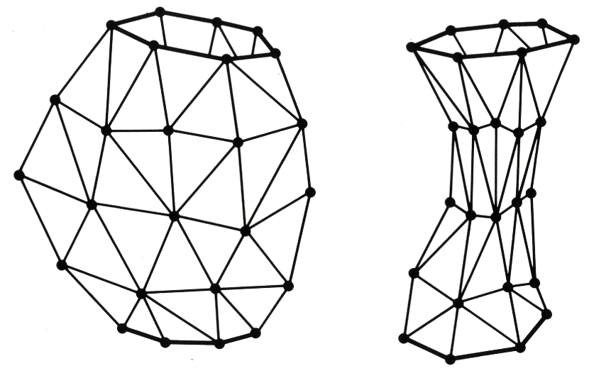
Figure 12: Two-dimensional simplicial geometries. Two-dimensional surfaces can be made up by joining together flat triangles to form simplicial manifold. A geometry of the surface is specified by an assignment of squared edge-lengths to the triangles. The figure shows two different geometries obtained by a different assignment of squared edge-lengths to the same simplicial manifold. The generalization of these ideas to four dimensions and Lorentz signature gives the natural lattice version of general relativity — the Regge calculus. In a sum-over-histories quantum theory of simplicial spacetimes, sums over geometries are represented by integrals over the squared edge-lengths. Diffeomorphism invariant alternatives can be defined by partitioning the space of allowed squared edge-lengths into exhaustive sets of exclusive regions. For example, one could partition closed cosmological geometries into the class that has no simplicial spacelike three surface greater than a certain volume and the class that has at least one such surface. In a given simplicial manifold it is possible to enumerate all three surfaces and identify the regions in the space of squared edge-lengths to which each class corresponds.

Simplicial manifolds provide the natural lattice version of general relativity and the most direct route to implementing a generally covariant cut-off. A surface in two dimensions can be built up from flat triangles as in a “geodesic dome”. The topology of the surface is specified by the way the triangles are joined together. A metric is specified by giving the squared edge-lengths of each triangle and a flat metric for its interior. In this way various two-dimensional simplicial geometries can be constructed (see Figure 12). The situation is similar in four dimensions. A geometry can be built up from flat, four-dimensional simplices. The topology of the simplicial manifold is specified by the way the simplices are joined together. A Lorentz metric is specified by giving the values of the $n_{1}$ squared edge lengths of the four-simplices, $s^{i}$, and a Lorentz signatured flat metric in their interiors. For the edge-lengths to be compatible with a Lorentz signatured flat metric, there must be some restrictions on the $s^{i}$ analogous to the triangle inequalities and $s^{i}$ will be negative if their edges define timelike directions. Values of a scalar field $\phi^{i}$ can be assigned to the $n_{0}$ vertices. The space of fine-grained histories for this simplicial approximation is then the domain of ${\bf R}^{n_{1}}\times{\bf R}^{n_{0}}$ consistent with the analogs of the triangle inequalities. A particular fine-grained history is a point in this space.

VIII.3 Coarse Grainings of Spacetime

Every assertion that we make about the universe corresponds to a partition of its histories into those for which the assertion is true and those for which it is false. If we assert that the universe is nearly homogeneous and isotropic on large scales at late times, we are utilizing a partition of the four-dimensional geometries into the class of those that are nearly homogeneous and isotropic at late enough times and the class of those that are not and asserting that our universe lies in the former class. Similarly, to say that the spacetime of the late universe behaves classically on accessible scales presumes that we can divide the cosmological histories into those correlated by Einstein’s equations in accessible coarse grainings and those which are not so correlated.

Even an assertion that refers to our own experience, such as the assertion that spacetime is nearly flat in the neighborhood of our sun, presumes a distinction of this form from the point of view of cosmology. To make the necessary partitions we would first have to describe what we mean by “our sun”. If we were kidnaped by aliens in UFO’s and set down again on a planet, how would we tell if it is our own earth and how would we tell if the star about which it orbits is our own sun? We would, of course, compare the planet of arrival to a description of the earth recorded in our memories. It is the remembered description that defines the physical situation that we mean by “our sun”. Utilizing such a description, it is possible to partition the histories into the classes that contain “our sun” with a nearly flat spacetime about it, the class that contains “our sun” with a highly curved spacetime, and the class that does not contain “our sun”. This is a coarse graining of the histories of the universe and a very coarse graining at that.

Thus, at a fundamental level every assertion about the universe, from assertions about large scale structure to statement about the everyday here and now, is the assertion that the history of the universe lies in the coarse-grained class in which the assertion is true and not in the class in which it is false. An assertion which does not unambiguously correspond to such a partition is not well defined. Generalized quantum mechanics predicts the probabilities for such alternative coarse-grained sets of histories.

Each of the examples of coarse graining discussed above is manifestly diffeomorphism invariant — no mention of coordinates went into their description. The allowed coarse grainings of this generalized quantum mechanics are more generally partitions of the fine-grained histories of metrics and matter field configurations into an exhaustive set of exclusive, diffeomorphism invariant classes. We now describe some further examples of partitions of four-metrics into diffeomorphism invariant classes.

A familiar question in quantum cosmology is “What are the probabilities of the possible maximum volumes the universe may reach in the course of its history?” The answer is of use, for example, in determining whether it is probable that a closed universe will be nearly spatially flat and exist for a long time – two features observed of our universe. We can state this question precisely utilizing a coarse graining that divides all four metrics into two diffeomorphism invariant classes $c_{0}$ and $c_{1}$ as follows:

• The class of metrics for which all spacelike three-surfaces have volumes less than a fiducial volume $V_{0}$.

• The class of metrics for each of which there is at least one three-surface with a volume larger than $V_{0}$.

This is a manifestly exhaustive set of exclusive diffeomorphism invariant alternatives. If it decoheres, the probability of $c_{0}$ is what we mean by the probability the the universe has a maximum volume not greater than $V_{0}$.

The following example illustrates that care must be used to choose coarse grainings that are genuine partitions of the set of fine-grained histories. It is sometimes suggested that one way of resolving the problem of time is to use some property of a three-surface, say, the total volume as a time variable. One could then define alternatives at a given value of total volume, say alternative possibilities for the rest of the three-geometry on that surface. However, this is not a genuine partition of the fine-grained histories because a given four-geometry may contain arbitrarily many three-surfaces of a given volume each with different three-geometries. This is the geometrical analog of paths which forward and backward in time, intersecting a surface of constant time more than once, which was discussed in the case of the reparametrization invariant models of Section VII.

The analogy with systems like the relativistic particle may be made somewhat more precise by utilizing a particular gauge and representing four-dimensional histories as curves in the superspace of three-dimensional geometries and matter field configurations (Figure 13). The analog of spacetime in the case of the relativistic particle is superspace in the case of spacetime geometry. Fine-grained histories of the relativistic particle are curves in spacetime. Fine-grained histories of spacetime geometry are curves in superspace. The analog of a surface of constant time in spacetime in the case of the relativistic particle would be a surface in superspace. For any surface one chooses in superspace there are fine-grained histories — spacetimes — that correspond to curves that intersect it an arbitrarily large number of times as was the case in the quantum mechanics of a single relativistic world line discussed in Section VII. Partitions by the location in superspace that a curve crosses a surface in superspace are therefore not possible. In this sense there is no property of three-geometry that can play the usual role of time in this generalized quantum mechanics.

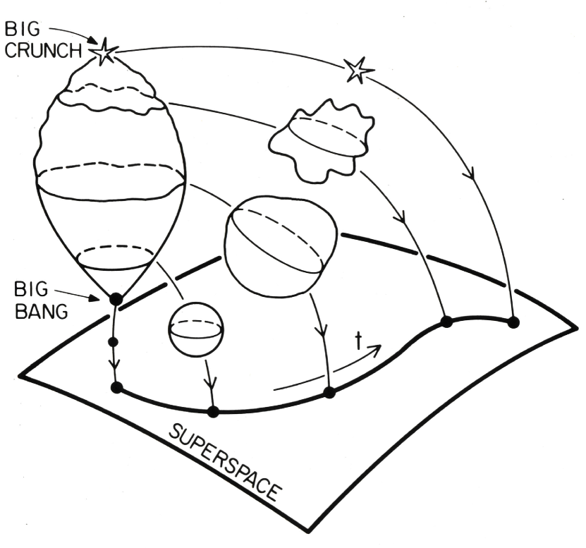
Figure 13: Superspace. A cosmological history is a four-dimensional cosmological spacetime with matter fields upon it. A two-dimensional representation of such a history is shown in the upper left of this figure proceeding from a big bang to a big crunch. In the Gaussian gauge of $ds^{2}=-dt^{2}+h_{ij}(x^{k},t)dx^{i}dx^{j}$ a cosmological history can be thought of as a parametrized succession of three-dimensional geometries and spatial matter field configuration. Superspace is the space of such three-dimensional geometries and matter field configurations. A “point” in superspace is a particular three-geometry and spatial matter field configuration. The succession of three-geometries and matter fields that make up a four-geometry and field history, therefore, trace out a path in superspace.

Allowed coarse grainings involving the geometries of spacelike surfaces can be constructed as follows: Define a range $R$ of three-geometries — a region in superspace — by a set of restrictions that are invariant under three-dimensional diffeomorphisms. For example, we might consider the region $R$ in which the total volume lies in a range $\Delta_{v}$ the integrated square of the three-dimensional Riemann tensor lies in another range $\Delta_{{\rm Riem}^{2}}$, and the average value of the scalar field lies in yet another range $\Delta_{\bar{\phi}}$. The fine-grained histories can be partitioned into the following two classes:   (1) the class of all histories that have no three surface in the region $R$, and   (2) the class of all histories that have at least one three surface in the region $R$. Such partitions are the analog of the partitions by a spacetime region discussed in Section V.3.2 for a non-relativistic particle and in Section VII.5.2 for a relativistic particle. By partitioning the paths according to their behavior with respect to many such regions of superspace a rich variety of coarse grainings analogous to the time sequences of non-relativistic quantum mechanics can be built up.

However, coarse grainings are not restricted just to those that distinguish the geometries of spacelike surfaces. For example, we could consider coarse-grainings by values of the proper four-volume in between spacelike surfaces or the values of the proper time on curves that connect spacelike surfaces.

The assumption that the fine-grained histories are continuous but not necessarily differentiable, means that some partitions of classical differentiable histories become vacuous like the partitions by finite values of the derivatives of the paths of a single particle discussed in Section V.4.2. Quantities like momenta, or the extrinsic curvature of surfaces, can still be defined utilizing a spacetime description, but only approximately. We shall return to what we might mean by a sum-over-non-differentiable geometries in connection with simplicial approximations below.

The general notion of coarse graining is by ranges of values of diffeomorphism invariant functionals of four-geometry and matter field configurations. These are especially easy to illustrate in the simplicial approximation described in Section VIII.2. Consider a fixed simplicial net as illustrated in Figure 12 and suppose that the fields and squared edge lengths are fixed on the two boundaries. The fine-grained histories are then specified by the values of the interior squared edge-lengths, $s^{i}$, and the field values, $\phi^{i}$, at the interior vertices. The general notion of coarse graining is by ranges of values of functions $F_{A}(s^{i},\phi^{i})$, $A=1,2,\cdots$ of the interior squared edge-lengths and field values that are invariant under any symmetry group of lattice that is a remnant of diffeomorphism invariance.

The main concluding point about the coarse grainings discussed here is that they supply a much larger set of diffeomorphism invariant alternatives for quantum cosmology than those conventionally contemplated on spacelike surfaces. Within this larger class are the coarse grainings that are directly accessible and easily interpretable by us.

VIII.4 The Decoherence Functional for General Relativity

In this section we shall describe a construction for the decoherence functional of general relativity. The essential ideas of the construction have already been illustrated in the gauge-invariant and reparametrization invariant models previously studied. As we mentioned in Section VI.1., general relativity exhibits both kinds of symmetry. It is necessary only to spell out the details of how the ideas illustrated in the models are combined.

VIII.4.1 Actions, Invariance, Constraints

The action for general relativity is a sum of the gravitational action for the metric and an action for the matter field

$$S[g,\phi]=S_{E}[g]+S_{M}[g,\phi]\,.$$ (358)

For illustrative purposes, we shall assume for the matter a scalar field with the action

$$S_{M}[g,\phi]=-{\textstyle{1\over 2}}\int_{M}d^{4}x(-g)^{\textstyle{1\over 2}}\left[(\nabla\phi)^{2}+V(\phi)\right]$$ (359)

for some potential $V(\phi)$. The action for Einstein’s theory that is appropriate when the three-metric, $h_{ij}$, is fixed on the boundaries of $M$ is

$$\ell^{2}S_{E}[g,\phi]=\int_{M}d^{4}x(-g)^{\textstyle{1\over 2}}(R-2\Lambda)+2\int_{\partial M}d^{3}xh^{\textstyle{1\over 2}}K$$ (360)

where $\ell=(16\pi G)^{\textstyle{1\over 2}}$ is $4\pi^{\textstyle{1\over 2}}$ times the Planck length. In the first integral, $R$ is the scalar curvature, $\Lambda$ is the cosmological constant and the integration range is the whole of the manifold $M$. The surface term is necessary to compensate for the second derivatives in the scalar curvature so as to make the action additive on spacetime regions. It is an integral over each boundary three-surface in which $h_{ij}$ is the metric induced by $g_{\alpha\beta}$ in the surface. The quantity $K$ is the trace of the extrinsic curvature of the surface , $K_{ij}$, defined as the projection into the surface of the derivative $-\nabla_{\alpha}n_{\beta}$ where $n_{\alpha}$ is the normal to the surface.

The canonical form of the action will be useful in constructing the functional integrals that define the decoherence functional because it is in phase-space that the measure for these integrals is most easily defined. We rapidly recall the canonical formulation. The first step is to write the action (360) in $3+1$ form using the $3+1$ decomposition of the metric with respect to a foliating family of spacelike surfaces that was discussed in Section VI.1. We assume that two members of the foliating family coincide with the boundary surfaces $\partial M^{\prime}$ and $\partial M^{\prime\prime}$. In terms of the lapse, shift, induced three-metric and extrinsic curvature of the constant $t$ surfaces, the action $S_{E}$ takes the simple form

$$\ell^{2}S_{E}\bigl{[}N,N^{i},h_{ij}\bigr{]}=\int_{M}dt\,d^{3}x\,h^{\textstyle{1\over 2}}N\ \left[K_{ij}K^{ij}-K^{2}-(2\Lambda-^{3}R)\right]\,.$$ (361)

Here, ${}^{3}R$ is the scalar curvature of the foliating surfaces and $K_{ij}$ is their extrinsic curvature. Explicitly

$$K_{ij}=(2N)^{-1}\left[-\dot{h}_{ij}+2D_{(i}N_{j)}\right]$$ (362)

where $D_{i}$ is the derivative in the three-dimensional constant-$t$ surfaces and the dot denotes a derivative with respect to $t$. The momenta conjugate to the $h_{ij}$ may be calculated straightforwardly from the action (361) and are

$$\ell^{2}\pi^{ij}=-h^{\textstyle{1\over 2}}\left[K^{ij}-h^{ij}K\right]\,.$$ (363)

The action (360) may then be reëxpressed in canonical form as

$$S_{E}\bigl{[}N,N^{i},\pi^{ij},h_{ij}\bigr{]}=\int\nolimits_{M}dt\,d^{3}x\left[\pi^{ij}\dot{h}_{ij}-NH(\pi^{ij},h_{ij})-N^{i}H_{i}(\pi^{ij},h_{ij})\right]\,,$$ (364)

where the $H$ and $H_{i}$ are defined as follows:

$$H = \ell^{2}G_{ijkl}\,\pi^{ij}\pi^{kl}+\ell^{-2}h^{\textstyle{1\over 2}}(2\Lambda-^{3}R)\,,$$ (365a)

$$H_{i} = -2D^{j}\pi_{ij}\,,$$ (365b)

with the DeWitt supermetric $G_{ijkl}$ being defined by

$$G_{ijkl}={\textstyle{1\over 2}}h^{-{\textstyle{1\over 2}}}\left(h_{ik}h_{jl}+h_{il}h_{jk}-h_{ij}h_{kl}\right)\,.$$ (366)

The evident symmetry with which the $(N,N_{i})$ and $(H,H_{i})$ enter (364) makes it useful to introduce the notation

$$N^{0}=N\ ,\ H_{0}=H$$ (367)

so that the canonical action can be rewritten compactly as

$$S_{E}\bigl{[}N^{\alpha},\pi^{ij},h_{ij}\bigr{]}=\int\nolimits_{M}dt\,d^{3}x\ \left[\pi^{ij}\dot{h}_{ij}-N^{\alpha}H_{\alpha}\right]\,.$$ (368)

The action for the matter field may be expressed in a canonical form similar to (364). In analogy to $h_{ij}({\bf x})$, we write $\chi({\bf x})$ for the value of the field on a constant-$t$ surface and $\pi_{\chi}({\bf x})$ for its conjugate momentum. For a scalar field $\chi({\bf x},t)=\phi({\bf x},t)$. The total action, $S_{E}+S_{M}$, takes the form

$$S\bigl{[}N^{\alpha},\pi^{ij},\pi_{\chi},h_{ij},\chi\bigr{]}=\int_{M}dt\,d^{3}x\ \left[\pi^{ij}\dot{h}_{ij}+\pi_{\chi}\dot{\chi}-N^{\alpha}{\cal H}_{\alpha}\bigl{(}\pi^{ij},\pi_{\chi},h_{ij},\chi\bigr{)}\right]\,.$$ (369)

Here, ${\cal H}_{0}$ and ${\cal H}_{i}$ are functions of the canonical coordinates and momenta defined by

$${\cal H}_{0} = H+h^{\textstyle{1\over 2}}T_{nn}\,,$$ (370a)

$${\cal H}_{i} = H_{i}+h^{\textstyle{1\over 2}}T_{ni}\,,$$ (370b)

where $T_{\alpha\beta}$ is the stress energy tensor of the scalar field expressed as a function of $\pi_{\chi},\chi$, and $h_{ij}$, an index $n$ indicating that it is projected onto the normal, $n^{\alpha}$, of the constant-$t$ surfaces, viz. $T_{ni}=n_{\alpha}T^{\alpha}_{i},\quad T_{nn}=n_{\alpha}T^{\alpha\beta}n_{\beta}$.

The absence of any term in (369) that is just a function of the coordinates and momenta and not proportional to lapse or shift is a signal of diffeomorphism invariance as we shall shortly see. Very little of the subsequent argument will depend on the specific forms of ${\cal H}_{0}$ and ${\cal H}_{i}$ beyond the fact that they are at most quadratic in the momenta. Almost everything we shall need follows from the form (369).

The diffeomorphism invariance of general relativity implies four constraints between the canonical coordinates $(h_{ij},\chi)$ and their conjugate momenta $(\pi^{ij},\pi_{\chi})$ as the general argument in Section VII.2. shows. With the action in the form (369), they are not difficult to find. They are the equations that result from extremizing (369) with respect to lapse and shift:

$${\cal H}_{\mu}\bigl{(}\pi^{ij}({\bf x}),\pi_{\chi}({\bf x}),h_{ij}({\bf x}),\chi({\bf x})\bigr{)}=0\,.$$ (371)

These four relations among the canonical coordinates and momenta are constraints that must be satisfied by any initial data for Einstein’s equation.

Dynamical equations in canonical form result from varying the action with respect to the canonical coordinates. For example, by varying with respect to $\pi^{ij}$ and $h_{ij}$ one finds

$$\dot{h}_{ij}({\bf x}) = N^{\mu}\left(\partial{\cal H}_{\mu}({\bf x})/\partial\pi^{ij}({\bf x})\right)\,,$$ (372)

$$\dot{\pi}^{ij}({\bf x}) = -N^{\mu}\left(\partial{\cal H}_{\mu}({\bf x})/\partial h_{ij}({\bf x})\right)\,,$$ (373)

and similar equations for the matter field and its momentum. The equations of motion may be written compactly by introducing the contraction

$${\cal H}(N)=\int_{t}d^{3}xN^{\mu}({\bf x}){\cal H}_{\mu}({\bf x})$$ (374)

and the Poisson bracket $\{~{},~{}\}$ with conventions such that $\{q^{A},p_{B}\}=\delta^{A}_{B}$. Then,

$$\dot{h}_{ij}({\bf x}) = \{h_{ij}({\bf x}),{\cal H}(N)\}\,,$$ (375a)

$$\dot{\pi}^{ij}({\bf x}) = \{\pi^{ij}({\bf x}),{\cal H}(N)\}\,,$$ (375b)

and similar equations for the matter degrees of freedom. Thus the constraints generate dynamics by specifying how the canonical coordinates change between two surfaces connected by lapse $N$ and shift $N^{i}$ (Figure 11). The constraints (371) together with the dynamical equations (375) are the Einstein equation written in canonical form.

The constraints of classical general relativity are closed under the Poisson bracket operation. That is, with all quantities evaluated on a common constant-$t$ surface

$$\left\{{\cal H}_{\mu}\left({\bf x}^{\prime}\right),{\cal H}_{\nu}\left({\bf x}^{\prime\prime}\right)\right\}=\int_{t}d^{3}x^{\prime\prime\,\prime}\ U^{\gamma}_{\mu\nu}\left({\bf x}^{\prime},{\bf x}^{\prime\prime},{\bf x}^{\prime\prime\,\prime}\right){\cal H}_{\gamma}\left({\bf x}^{\prime\prime\,\prime}\right)\,.$$ (376)

The structure functions, $U^{\gamma}_{\mu\nu}$, involve various $\delta$-functions, derivatives and the metric $h_{ij}$. Their explicit form, which will not be necessary for us, can be found in many standard references (e.g. Kuc74 , p. 250).

Closure of the constraints under the Poisson bracket operation is necessary for consistency. Otherwise the Poisson bracket of two constraints would represent new and different constraints on the canonical coordinates. However, because the structure functions depend on the coordinates (specifically the $h_{ij}$), the relations (376) do not define an algebra (although they are often referred to informally as such). In particular, they do not define the algebra of four-dimensional diffeomorphisms that were the origin of the constraints and that fact has important consequences for the canonical theory.

A straightforward calculation shows that the action (369) is invariant under the following canonical transformation generated by an infinitesimal vector $\epsilon^{\alpha}({\bf x})$:

$$\delta h_{ij}({\bf x}) = \left\{h_{ij}({\bf x}),{\cal H}(\epsilon)\right\}\,,$$ (377a)

$$\delta\pi^{ij}({\bf x}) = \{\pi^{ij}({\bf x}),{\cal H}(\epsilon)\}\,,$$ (377b)

$$\delta\chi({\bf x}) = \{\chi({\bf x}),{\cal H}(\epsilon)\}\,,$$ (377c)

$$\delta\pi_{\chi}({\bf x}) = \left\{\pi_{\chi}({\bf x}),{\cal H}(\epsilon)\right\}\,,$$ (377d)

together with the related transformation of the lapse and shift:

$$\delta N^{\alpha}({\bf x})=\dot{\epsilon}^{\alpha}({\bf x})-\int_{t}d^{3}x^{\prime}\int\nolimits_{t}d^{3}x^{\prime\prime}U^{\alpha}_{\beta\gamma}\left({\bf x}^{\prime},{\bf x}^{\prime\prime},{\bf x}\right)N^{\beta}\left({\bf x}^{\prime}\right)\epsilon^{\gamma}\left({\bf x}^{\prime\prime}\right)\,,$$ (377e)

where all functions are evaluated on a common constant-$t$ surface. These are the generalizations of the symmetries (273) in the case of the relativistic world line. The action (369) is invariant under the transformations (377) provided, as stressed by Teitelboim Tei83a , that the normal component of $\epsilon^{\mu}$, vanishes on all components of the boundary of $M$.

The infinitesimal symmetry (377) of the canonical action is closely connected with diffeomorphism invariance but does not coincide with it BK72 ; LW90 . Indeed, the two symmetries act on different spaces. The canonical symmetry acts on the space of extended phase-space histories, while diffeomorphisms act on the space of four-dimensional metrics and field configurations. Under an infinitesimal diffeomorphism generated by a vector field $\xi^{\mu}(x)$, the metric and matter field change by

$$\delta g_{\alpha\beta}(x) = 2\nabla_{(\alpha}\xi_{\beta)}(x)\,,$$ (378a)

$$\delta\phi = \xi^{\alpha}(x)\nabla_{\alpha}\phi(x)\,.$$ (378b)

Equations (378) coincide with the transformations of three-metric and lapse given by (377a) if the components of $\epsilon^{\mu}$ are identified with the normal component and the projection of $\xi^{\mu}$ into the surface as follows

$$\xi^{0}=\epsilon^{0}/N,\,\,\quad\xi^{i}=\epsilon^{i}-N^{i}\epsilon^{0}/N\,.$$ (379)

provided that the equations of motion relating the time derivatives of canonical coordinates to momenta are satisfied. The infinitesimal canonical symmetry (377) thus coincides with diffeomorphism invariance only when certain (not all) of the equations of motion are satisfied. However, for theories with constraints that are at most quadratic in the momenta these equations of motion are effectively satisfied in path integral constructions at least for gauge conditions that do not restrict the momenta. Gaussian integrals over the momenta effectively replace the $\pi$’s by the right combinations of $\dot{q}$’s, and integrals over exponents linear in the momenta lead to $\delta$-functions that enforce the relevant relation exactly. It’s important to keep in mind, however, that the relation (379) holds only when both $\xi^{\mu}$ and $\epsilon^{\mu}$ are infinitesimal and will fail, for example, near $N=0$. The quantities $\epsilon^{\mu}$ must therefore be further restricted to coincide with diffeomorphisms than just invariance of the canonical action under (377) would require. Further restrictions are needed to ensure that the resulting $\xi^{\mu}$ correspond to one-to-one mappings of the manifold into itself. For these reasons, the symmetries generated by (377) are a larger set than the diffeomorphisms which they include BK72 ; LW90 . For general relativity, therefore, we may use invariance under the infinitesimal canonical symmetry to ensure invariance of the measure under infinitesimal diffeomorphisms.

VIII.4.2 Class Operators

The construction of the class operators corresponding to the coarse grainings discussed in VIII.3 follows that for gauge theories and models with a single reparametrization invariance. As discussed in VIII.2 the fine-grained histories are metrics and matter fields on the manifold $M$ bounded by the two boundaries $\partial M^{\prime}$ and $\partial M^{\prime\prime}$. The Hilbert space in which the class operators act is therefore formally the space ${\cal H}^{(h,\chi)}$ of square integrable functionals of three-metrics and matter field configurations on these boundary surfaces. We therefore define

$$\bigl{\langle}h^{\prime\prime}_{ij},\chi^{\prime\prime}\left\|C_{\alpha}\right\|h^{\prime}_{ij},\chi^{\prime}\bigr{\rangle}=\int_{\alpha}\delta\pi\delta h\delta\pi_{\chi}\delta\chi\delta N$$

$$\times\Delta_{\Phi}\bigl{[}h_{ij},\pi^{ij},\chi,\pi_{\chi},N^{\gamma}\bigr{]}\ \delta\bigl{[}\Phi^{\beta}\bigl{[}h_{ij},\chi,N^{\gamma}\bigr{]}\bigr{]}\exp\bigl{\{}iS\bigl{[}N^{\gamma},\pi^{ij},\pi_{\chi},h_{ij},\chi\bigr{]}\bigr{\}}$$ (380)

where $S$ is the canonical action of (369) and the integral is over all metrics $g_{\mu\nu}(x)=(N^{\beta}({\bf x},t),h_{ij}({\bf x},t))$ and field configurations $\phi(x)=\chi({\bf x},t)$ that lie in the diffeomorphism invariant class $c_{\alpha}$. A few words are of course in order about the rest of (380) and about the attitude we shall adopt towards such formal expressions. $\Phi^{\beta}$ stands for four conditions that fix the four-dimensional symmetry (377) and $\Delta_{\Phi}$ is the associated “Faddeev-Popov factor”. These conditions are assumed to leave the momenta unrestricted so they may be formally integrated out. The important remainder of (380) is the “measure”. This is assumed to be the canonical (Liouville) measure in the canonical coordinates $(h_{ij}({\bf x}),\chi({\bf x}))$ and their conjugate momenta $(\pi^{ij}({\bf x}),\pi_{\chi}({\bf x}))$. This measure is formally invariant under infinitesimal canonical transformations generated through Poisson brackets. In particular it is invariant under transformations (VIII.4.20a–d) that include infinitesimal diffeomorphisms in the sense discussed in Section VIII.4.1.

The only remaining choice needed to specify the class operators is the range of integration of the multipliers. We integrate the shifts, $N^{i}(x)$, over ${\bf R}$ at each point $x$. We integrate the lapse, $N(x)$, over a positive range for each point $x$. This is a diffeomorphism invariant range because the $3+1$ decomposition of the metric depends only on $N^{2}$ [cf. (206)]. All metrics are therefore represented as $N$ ranges over positive values. A positive range is not, however, invariant under the larger group of transformations (VIII.4.20a–d) that leave the canonical action and measure invariant.

With a positive lapse range, if the symmetry fixing conditions $\Phi^{\beta}$ are chosen to be independent of $\pi^{ij}$, these momenta can be formally integrated out of the matrix elements of the class operators since the action is quadratic in the $\pi^{ij}$ and the partition $\{c_{\alpha}\}$ does not restrict them. The result is a path integral in Lagrangian form

$$\left\langle h^{\prime\prime},\chi^{\prime\prime}\left\|C_{\alpha}\right\|h^{\prime},\chi^{\prime}\right\rangle=\int_{\alpha}\delta h\delta\phi\delta N\Delta_{\Phi}\left[h,\phi,N\right]\,\delta\,\left[\Phi\left[h,\phi,N\right]\right]\exp\left\{iS\left[N,h,\phi\right]\right\}.$$ (381)

Here we have compressed the notation of (380) even further by omitting indices on vectors and tensors. The “measure” is that induced by the Liouville measure on phase space. The action is the usual Lagrangian action for general relativity (361) coupled to matter.

The choice of a positive range for the lapse $N$ was advocated by Teitelboim Tei83d in his pioneering study of canonical path integrals for general relativity and has a number of compelling arguments in its favor. First, as we saw in Section VII, in the case of a relativistic particle interacting with an external potential, the choice of positive multiplier range reproduces the usual $S$-matrix elements of the corresponding field theory. Second, and perhaps more persuasively, the choice of a positive range for $N$ corresponds in four-dimensional, geometrical terms to a direct implementation of Feynman’s sum-over-histories principles for quantum mechanics HH91 . To see this, note that in the $3+1$ form of the action (361), $\sqrt{-g}$ is represented as $Nh^{1/2}$. The integral (381) over a positive range for $N$ can therefore be reexpressed as

$$\left\langle h^{\prime\prime},\chi^{\prime\prime}\left\|C_{\alpha}\right\|h^{\prime},\chi^{\prime}\right\rangle=\int_{\alpha}\delta g\,\delta\phi\,\Delta_{\Phi}[g,\phi]\,\delta[\Phi[g,\phi]]\ \exp(iS[g,\phi])$$ (382)

where $g$ and $\phi$ denote the four-dimensional metric and matter field configuration respectively. Reversal of the sign of $N$ in (361) changes the sign of the action. A sum over both positive and negative lapse therefore corresponds, not to sum over geometries weighted by $\exp(iS)$, but rather by $\cos(S)$. This choice would define a distinct generalized quantum mechanics, but positive lapse and (382) are closer to Feynman’s original principle.

VIII.4.3 Adjoining Initial and Final Conditions

The rest of the construction of the decoherence functional for a quantum theory of spacetime parallels that for theories with a single reparametrization invariance discussed in Section VII. Initial and final conditions are represented by wave functions that satisfy the constraints on the superspace of three-metrics and spatial matter field configurations. For example, the initial condition might be represented by a family of wave functions $\{\Psi_{j}[h_{ik}({\bf x}),\chi({\bf x})]\}$ that each satisfy

$${\cal H}_{\mu}\left[\widehat{\pi}^{ik}({\bf x}),\widehat{\pi}_{\chi}({\bf x}),h_{ik}({\bf x}),\chi({\bf x})\right]\Psi_{j}\left[h_{ik}({\bf x}),\chi({\bf x})\right]=0\,.$$ (383)

Here, we take $\widehat{\pi}^{ij}({\bf x})=-i\delta/\delta h_{ij}({\bf x})$, $\widehat{\pi}_{\chi}({\bf x})=-i\delta/\delta\chi({\bf x})$ and the ${\cal H}_{\mu}$ are operators constructed from these quantities and the three-metric and scalar field that represent the classical constraints (371). Simply writing these equations down should not obscure the fact that there are serious problems to be faced with giving them a precise meaning. For instance, eq. (383) is not just four equations but four functional differential equations for each point on the manifold $M^{3}$. The formal products of operators that occur in ${\cal H}_{\mu}$ are singular and must be regulated TW87 . Even given a regularization there is the delicate question of finding an operator ordering such that the constraints obey the “algebra” expected from the classical algebra of Poisson brackets (376). We do not solve these problems here.

The next step in constructing the decoherence functional is to attach the wave functions satisfying (383) representing initial and final conditions to the class operator matrix elements in analogy with (VII.1.8) for reparametrization invariant theories. We write

$$\left\langle\Phi_{i}\left|C_{\alpha}\right|\Psi_{j}\right\rangle=\Phi_{i}\left[h^{\prime\prime},\chi^{\prime\prime}\right]\,\circ\,\left\langle h^{\prime\prime},\chi^{\prime\prime}\left|C_{\alpha}\right|h^{\prime},\chi^{\prime}\right\rangle\,\circ\,\Psi_{j}\left[h^{\prime},\chi^{\prime}\right]$$ (384)

where $\circ$ is a Hermitian inner product between functionals on superspace although not necessarily a positive definite one. We shall return to a discussion of candidates for this product in a moment, but first we complete the construction of the decoherence functional. Specify a set of initial wave functions $\{\Psi_{j}[h,\chi]\}$ together with their probabilities $\{p^{\prime}_{j}\}$. Specify a set of final wave functions $\{\Phi_{i}[h,\chi]\}$ together with their probabilities $\{p^{\prime\prime}_{i}\}$. Construct

$$D\left(\alpha^{\prime},\alpha\right)={\cal N}\sum_{ij}p^{\prime\prime}_{i}\left\langle\Phi_{i}\left|C_{\alpha^{\prime}}\right|\Psi_{j}\right\rangle\ \left\langle\Phi_{i}\left|C_{\alpha}\right|\Psi_{j}\right\rangle^{*}p^{\prime}_{j}\,.$$ (385)

With an appropriate choice for the constant ${\cal N}$ this satisfies the requirements (i)–(iv) of (117) for a decoherence functional of a generalized quantum mechanics. It is Hermitian with positive diagonal elements whether or not the product $\circ$ is positive. The linearity of the sums over histories that define the class operators $C_{\alpha}$ ensures the consistency with the principle of superposition. Normalization fixes ${\cal N}$ as

$${\cal N}^{-1}=\sum_{ij}p^{\prime\prime}_{i}\left|\left\langle\Phi_{i}\left|C_{u}\right|\Psi_{j}\right\rangle\right|^{2}p^{\prime}_{j}$$ (386)

where $C_{u}$ is defined by the unpartitioned sum over all histories in (382). The decoherence functional (385) is thus a natural basis for defining decoherence and probabilities in a generalized quantum mechanics of coarse-grained histories of spacetime geometry and matter fields.

There remains the specification of the inner product $\circ$ and the specification of initial and final conditions in particular quantum cosmologies. We consider the product in the rest of this subsection and particular initial and final conditions in the next.

A positive, Hermitian, covariant, inner product between wave functions on superspace that are annihilated by the constraints has been sought in the Dirac approach to the quantization of general relativity for nearly the past forty years. The problem is with the positivity. Squaring and integrating over all of superspace does not provide a suitable inner product because, like the case of the relativistic particle, the constraints of general relativity imply a conserved current in superspace DeW67 . This conserved current means that wave functions that satisfy the constraints are not necessarily normalizable when squared and integrated over all of superspace with a measure that makes the operators representing the constraints Hermitian [cf. the discussion following VII.3.15]. There is an analog of the conserved Klein-Gordon product on surfaces in superspace. It is usually called the DeWitt product and we shall exhibit it shortly. However, like the Klein-Gordon product, the DeWitt product is not generally positive and therefore cannot serve as the basis for an inner product defining a Hilbert space in which the norm of a state vector is related to probability.

In free field theory in flat background spacetimes, the Klein-Gordon inner product is positive on positive frequencies solutions of the constraint. The existence of timelike Killing fields for the underlying flat spacetime allows a notion of positive frequency to be consistently specified over the whole of spacetime. Time translation invariance means positive frequency solutions of the Klein-Gordon equation at one time remain positive frequency solutions at all times. A single particle Hilbert space can thus be constructed for a free relativistic particle. This free particle construction does not extend to particles interacting with a potential and neither is it available in general relativity for there are no Killing fields in superspace Kuc81 .

It may be that a deeper investigation into the constraints of general relativity will reveal a positive, Hermitian, covariant, inner product on solutions to the constraints. That is the aim of some. If found, it could be used to construct a decoherence functional for a quantum theory of spacetime via (385) and (384). Here, however, we shall follow a different route. This is to note that in the present framework the wave functions that satisfy the constraints and specify the initial and final conditions do not have a direct probability interpretation. That is provided by the decoherence functional. The spaces of wave functions specifying the initial and final conditions therefore do not need a Hilbert space structure. We are therefore free to take a non-positive product for $\circ$ and still have positive probabilities for decoherent sets of coarse-grained histories. The DeWitt product naturally suggests itself and in the following we spell out what it is and what the consequences of using it are.

By “superspace”, ${\cal M}$, we mean the space of three-metrics $h_{ij}({\bf x})$ and spatial matter field configurations $\chi({\bf x})$ on a spacelike surface of topology $M^{3}$. ${\cal M}$ is the product of ${\cal M}_{h}$, the space of three-metrics, and ${\cal M}_{\chi}$, the space of spatial matter field configurations. ${\cal M}_{h}$ may be thought of as the product of the six-dimensional space of metric coefficients $h_{ij}({\bf x})$ at each point ${\bf x}$ of $M^{3}$. Similarly, ${\cal M}_{\chi}$ may be thought of as the product of the one-dimensional space of field values $\chi({\bf x})$ at each point $\bf x$ of $M^{3}$. The formal cardinality of ${\cal M}$ is therefore $\infty^{3(6+1)}$ where $\infty$ denotes cardinality of the real line.

The DeWitt metric $G_{ijkl}({\bf x})$ was introduced in (366) and provides an inner product on the six-dimensional space of three-metrics at a point ${\bf x}$. To find an explicit expression, one can think of a correspondence between the six dimensions and the six possible symmetric pairs of indices $i$ and $j$, but it is easier to write expressions directly in terms of the usual three-dimensional tensor indices. Thus, for example, the inverse of $G_{ijkl}$ is defined by

$$\bar{G}^{ijkl}G_{klmn}={\textstyle{1\over 2}}\left(\delta^{i}_{m}\delta^{j}_{n}+\delta^{i}_{n}\delta^{j}_{m}\right)$$ (387)

and is

$$\bar{G}^{ijkl}={\textstyle{1\over 2}}h^{\textstyle{1\over 2}}\left(h^{ij}h^{kl}+h^{il}h^{jk}-2h^{ij}h^{kl}\right)\,.$$ (388)

The inner product between two vectors $\delta h^{1}_{ij}({\bf x})$ and $\delta h^{2}_{ij}({\bf x})$ tangent to superspace at ${\bf x}$ is then

$$\bar{G}^{ijkl}({\bf x})\,\delta h^{1}_{ij}({\bf x})\delta h^{2}_{ij}({\bf x})\,.$$ (389)

The inner product on the whole of ${\cal M}_{h}$ is the sum of these inner products over positions ${\bf x}$,

$$(\delta h^{1},\delta h^{2})=\int_{M^{3}}d^{3}x\ \bar{G}^{ijkl}({\bf x})\delta h^{1}_{ij}({\bf x})\delta h^{2}_{ij}({\bf x})\,.$$ (390)

In a similar way on ${\cal M}_{\chi}$ we can put

$$(\delta\chi^{1},\delta\chi^{2})=\int_{M^{3}}d^{3}xh^{\textstyle{1\over 2}}\,\chi^{1}({\bf x})\chi^{2}({\bf x})\,.$$ (391)

Thus superspace, ${\cal M}$, acquires a metric structure.

The DeWitt metric is not positive definite. Of six orthogonal directions at a point, one will be timelike and five will be spacelike. Conformal deformations of the metric,

$$\delta h_{ij}({\bf x})=\delta\lambda({\bf x})h_{ij}({\bf x})$$ (392)

are timelike, for instance. We can therefore define a notion of a “spacelike surface” $\sigma$ in ${\cal M}$. For example, we might fix the value of the determinant of the three-metric, $h({\bf x})$, at each point. The DeWitt metric provides a notion of volume element $d\Sigma_{ij}({\bf x})$ in such a surface at each ${\bf x}$. Using this the DeWitt product between wave functionals on superspace $\Psi^{1}[h,\chi]$ and $\Psi^{2}[h,\chi]$ can be defined formally as

$$\Psi^{1}\circ\Psi^{2}=iZ\int_{\sigma}\Psi^{1*}[h_{ij}({\bf x}),\chi({\bf x})]\left[\prod\limits_{\bf y}\left(d\chi({\bf y})\,d\Sigma_{kl}({\bf y})\right)\frac{\buildrel\leftrightarrow\over{\delta}}{\delta h_{kl}({\bf y})}\right]\Psi^{2}\left[h_{ij}({\bf x}),\chi({\bf x})\right].$$ (393)

A constant factor $Z$ has been included in (393) to absorb divergences arising from the fact that wave functionals satisfying the constraints are constant on orbits of the diffeomorphisms of $M^{3}$ in superspace. This constant will cancel in the construction of probabilities if the DeWitt product is used to construct the decoherence functional as described above. Alternatively, the product could be defined with suitable gauge fixing machinery.

The DeWitt product defined by (393) is the formal analog in superspace endowed with the DeWitt metric of the Klein-Gordon product in spacetime with the Minkowski metric. Like the Klein-Gordon inner product it is not positive. Like the Klein-Gordon product, the DeWitt product is formally independent of the surface $\sigma$ provided $\Psi^{1}$ and $\Psi^{2}$ are solutions of the Wheeler-DeWitt equation. In the construction of the decoherence functional the wave functions specifying the initial and final conditions are assumed to satisfy the Wheeler-DeWitt equation. The class operator matrix elements satisfy the same equation in each argument in the neighborhood of surfaces $\sigma^{\prime}$ and $\sigma^{\prime\prime}$ that are outside the restrictions of the coarse graining. Thus, at a formal level, surface independence for the spacetime decoherence functional is achieved in the same way that it is for the relativistic world line.

An important difference between this generalized quantum mechanics of spacetime and that for the relativistic world line in flat spacetime described in Section VII concerns the space of wave functionals describing initial and final conditions. In the case of the relativistic particle, the choice of the range $N>0$ meant that the matrix elements $\langle x^{\prime\prime}\|C_{\alpha}\|x^{\prime}\rangle$ contained only positive frequencies in their time variation with respect to any direction defined by a timelike Killing vector of flat spacetime. As a consequence, the wave functions describing initial and final conditions could be restricted to the linear space of positive frequency solutions of the Klein-Gordon equations without loss of generality. The Klein-Gordon product is positive for such positive frequency solutions making that space a Hilbert space. The quantum mechanics of spacetime described here retains the positive range for the lapse integration. However, this does not correspond to a notion of positive frequency for solutions of the Wheeler-DeWitt equation because there are generally no Killing vectors on superspace. The space of initial or final wave functions endowed with the DeWitt product is not, therefore, a Hilbert space.

VIII.5 Discussion — The Problem of Time

The specification of the decoherence functional (385) completes the formulation of a generalized sum-over-histories quantum mechanics for spacetime geometry suitable for application to cosmology. Fine-grained histories are manifolds, metrics and matter field configurations. Sets of alternative coarse-grained histories are diffeomorphism-invariant partitions of these. The decoherence functional defines a notion of interference between coarse-grained histories that is consistent with the principle of superposition. Given initial and final conditions, this decoherence functional can be used to determine which sets of coarse-grained histories of the universe can be assigned consistent probabilities, and what those probabilities are, according to the principles of generalized quantum mechanics described in Section IV.

This is a fully four-dimensional formulation of a quantum mechanics of spacetime. Fine-grained histories are four-dimensional metrics and field configurations. Four-dimensional alternatives are defined by partitions of these fine-grained histories into classes that are invariant under four-dimensional diffeomorphisms. Dynamics is specified in the decoherence functional by sums over four-dimensional histories involving a four-dimensional diffeomorphism invariant action and measure.

This is a generally covariant formulation of the quantum mechanics of spacetime. No additional ingredients beyond the metric and field configurations were needed to specify either fine- or coarse-grained histories. In particular no preferred sets of spacelike surfaces in superspace or spacetime were singled out in the construction of the decoherence functional. We have a quantum mechanics of spacetime that is free from the problem of time.

Can this four-dimensional sum-over-histories quantum mechanics be reformulated as a quantum mechanics of states on spacelike surfaces in superspace and their unitary evolution by a Hamiltonian or by state vector reduction? It seems unlikely. The standard reconstruction of Hamiltonian quantum mechanics from a sum-over-histories formulation involves identifying a family of surfaces in the space of coordinates which each history intersects once and only once. (See the discussion in Section IV.4). For gravity this would mean a set of surfaces in superspace that each geometrical history intersects once and only once. That would define a quantity that would uniquely label a set of spacelike surfaces in every possible cosmological four-geometry. While there may be such quantities for certain classical spacetimes satisfying the Einstein equation MT80 , there are none for a general four-dimensional cosmological geometry. A general cosmological geometry, for example, could have arbitrarily many surfaces of a given three-volume or trace of the extrinsic curvature. As in the case of the theory of a relativistic particle without a preferred time, we are unlikely to be able to formulate this generalized sum-over-histories quantum mechanics in terms of states on spacelike surfaces. There is no preferred time with which to do so.

We should probably stress that the use of wave functions to specify initial and final conditions or the use of functional integrals to define them is not to be construed as a definition of a notion of state on a spacelike surface. In the present framework, these wave functions generally have no direct probability interpretation. Rather, they are part of the specification of the decoherence functional which determines the probabilities of decoherent spacetime alternatives as we have described.

Of course, were general covariance broken at the quantum mechanical level so that the fine-grained histories were restricted to those in which some superspace quantity uniquely labeled a foliating family of spacelike surfaces in every possible spacetime, then it would be still possible to construct a generalized quantum mechanics according to the principles we have described. It would have as its starting point the more restricted set of histories which were foliable by the quantity involved. Its construction would be analogous to the formulation of the quantum mechanics of a relativistic particle with the preferred time of a particular Lorentz frame that was discussed in Section VII.4. As there, an equivalent formulation in terms of states on the corresponding surfaces in superspace would be expected. It is important to note that such restrictions imply a definite physical prediction. To restrict the fine-grained histories, for example, to a set where a type of surface of a given three-volume occurs once and only once is to predict that once that volume occurs there is zero probability for it ever to occur again.

A generalization of Hamiltonian quantum mechanics, such as that of this section, which dispenses with the familiar notion of “state on a spacelike surface” has the heavy obligation to show how it is recovered again in a suitable limit. We shall discuss this question in Section IX. There we shall argue that, in those limiting situations where spacetime behaves classically, we recover from this generalized quantum mechanics of spacetime geometry and matter fields an approximate quantum mechanics of matter fields in which the preferred time necessary for a formulation in terms of states is supplied by the background classical geometry.

VIII.6 Discussion – Constraints

Are the constraints satisfied in this generalized quantum mechanics for general relativity? In the cases of electromagnetism and the relativistic world line, we were able to give two distinct meanings to the question of whether the constraints were satisfied. The first was to partition the histories by the values of the constraints and ask whether the probability was unity that they were satisfied. The second was to ask whether class operators commuted with the constraints and whether branch wave functions were annihilated by them. In this subsection we offer some thoughts on these questions in the quantum mechanics of general relativity we have constructed.

In the case of electromagnetism and the relativistic world line the constraints restricted the values of certain combinations of the momenta. The restrictions were $\pi^{L}({\bf x})=0$ in the case of electromagnetism and $p^{2}=-m^{2}$ in the case of the relativistic world line. We were able to give meaning to a partition of the histories by the values of $\pi^{L}({\bf x})$ and $p^{2}$ by defining the momenta as partitions by “displacements in flight” in the limit of very long intervals of time. We found vanishing probability for values of the momenta that did not satisfy the constraints. In this physical sense, the theories could be said to imply the constraints with probability unity.

To assess the probability that the constraints are satisfied in the present quantum mechanics of spacetime, we must first exhibit a diffeomorphism-invariant partition of metrics and field configurations into a class where the constraints are satisfied and a class where they are not. This is a more difficult problem than exhibiting similar partitions in the cases of gauge theories or the relativistic world line for two reasons: First, the constraints are not combinations of the momenta alone when written in the form of (370) and (365), so that identifying the spacetime metrics in which they are satisfied approximately is not a question resolved as straightforwardly as with the “time of flight” constructions in the simpler examples. (Remember the fine-grained histories are not generally differentiable!) Second, the partition must include a diffeomorphism invariant specification of the spacelike surfaces on which the constraints are to be investigated. We cannot, for example, usefully partition the fine-grained histories into the class in which the constraints are defined and satisfied on every spacelike surface and the class in which they are not. If a geometry satisfies the constraints on every spacelike then it solves the Einstein equation Kuc81b . A partition into classical histories and non-classical ones is diffeomorphism invariant but also trivial in quantum mechanics. Rather, it is necessary to investigate the constraints on some specific family of spacelike surfaces. One could perhaps imagine, in analogy with the relativistic world line, specifying such a family using distances along suitable curves from $\partial M^{\prime}$. However, such partitions are not likely to be of much use in practical quantum cosmology. We shall not pursue them further here.

We can more readily investigate the questions of whether class operators commute with operator versions of the constraints in the “Hilbert space” of functionals of three-metrics and whether branch wave functionals corresponding to individual histories in a coarse-grained set are annihilated by operator forms of the constraints. For simplicity, we confine the discussion to the case of pure gravity.

We first must draw a distinction between the momentum constraints $H_{i}=0$ and the Hamiltonian constraint $H=0$ in the notation of (365). In the 3+1 decomposition through which they are defined, the momentum constraints generate three-dimensional diffeomorphisms in the sense that

$$h_{ij}+\xi^{k}\{h_{ij},H_{k}\}=h_{ij}+D_{i}\xi_{j}+D_{j}\xi_{i}\,.$$ (394)

The Hamiltonian constraint, on the other hand, generates changes more analogous to reparametrization transformations.

For the reparametrization-invariant relativistic world line discussed in Section VII.6, class operators neither generally commuted with the constraint nor were branch wave functions annihilated by them. We can hardly expect more for the Hamiltonian constraint in general relativity for similar reasons. However, the momentum constraints generate three-dimensional diffeomorphisms that are the analogs of spatial gauge transformations in electromagnetism. The same argument that showed that, when defined with a certain class of gauge-fixing conditions, the class operators corresponding to gauge invariant partitions in electromagnetism commuted with the $\pi^{L}({\bf x})$ can be generalized to show a similar result for the momentum constraints in general relativity (although we shall not give the details here). A notion of a branch wave functional may be defined by

$$\Psi_{\alpha}[h_{ij}]=\langle h_{ij}\|C_{\alpha}|\Psi\rangle=\langle h_{ij}\|C_{\alpha}\|h^{\prime}_{ij}\rangle\circ\Psi[h^{\prime}_{ij}]\,.$$ (395)

Then, provided that the surface $\sigma^{\prime}$ on which the $\circ$ product is calculated is itself defined by a three-dimensional diffeomorphism invariant condition, and provided the matrix elements of $C_{\alpha}$ are defined with invariant gauge-fixing conditions as described above, one can show formally that

$$H_{i}({\bf x})\Psi_{\alpha}[h_{ij}]=0\,.$$ (396)

Only in such a circumscribed way can have we been able to make limited contact with the ideas of Dirac quantization.

VIII.7 Simplicial Models

In the absence of any conclusive evidence that its defining functional integrals converge, the generalized quantum mechanics for spacetime described in the preceding three subsections must be regarded as a formal construction for the moment. Whether the Einstein action can be used as the starting point for a complete, finite, manageable quantum theory of gravity in which the ingredients of the above framework can be given concrete meaning is at best an open question. Therefore, to investigate the decoherence and calculate the probabilities of the alternative histories of our universe that might be confronted with observation, we must either find the correct quantum theory of gravity or retain the Einstein action but turn to finite models in which its ultraviolet divergences have been cut off. This second approach will be useful if, for a realistic initial condition, the predictions of very low energy phenomena, such as the probabilities of various galaxy-galaxy correlation functions at the present epoch, are insensitive to this cut-off. This subsection describes (very briefly) a class of such finite models based on the simplicial approximation to smooth geometries and the methods of the Regge calculus.

As mentioned in Section VIII.2, a simplicial four-manifold can be constructed by joining together four-simplices — the four-dimensional analogs of triangles in two-dimensions. A metric on such a simplicial manifold is specified by assigning definite values to the squared lengths of the edges and a flat metric consistent with these values to the interior of the simplices. Both Lorentzian and Euclidean geometries can be represented in this way, the signature in each simplex being determined by the values of its squared edge-lengths. Euclidean geometries have all positive squared edge-lengths that satisfy the higher dimensional analogs of the triangle inequalities. Lorentzian geometries may have some negative (timelike) squared edge-lengths and are restricted by analogous inequalities. Thus, geometry is represented discretely and finitely. Matter field configurations can also be represented discretely, for example, in the case of a scalar field by specifying the value of the field at each vertex.

In four-dimensions, the curvature of a simplicial geometry is concentrated on the triangles in the same way that curvature in a two-dimensional simplicial surface is concentrated at the vertices. The deficit angle, $\theta$, is a measure of the curvature. In two dimensions, the deficit angle of a vertex is the difference between $2\pi$ and the sum of the interior angles between edges meeting at that vertex. In four dimensions, the deficit angle of a triangle is $2\pi$ minus the sum of the dihedral angles between the three-simplices that meet in that triangle. A flat geometry has vanishing deficit angles.

Einstein’s action (360) has a beautifully simple, geometrical expression for a simplicial geometry. It is most straightforwardly stated for a Euclidean geometry. The form for a Lorentzian geometry, can be found by analytic continuation of the squared edge-lengths to the values that specify a Lorentzian signatured geometry. The Euclidean action is Reg61 ; HS81

$$\ell^{2}I=-\sum_{\scriptstyle{\rm interior}\atop\scriptstyle{\rm triangles}}2A\theta+\ \sum\limits_{\scriptstyle{\rm four-}\atop\scriptstyle{\rm simplices}}2\Lambda V_{4}-\sum_{\scriptstyle{\rm boundary}\atop\scriptstyle{\rm triangles}}2A\psi\,.$$ (397)

The first two terms correspond to the scalar curvature and cosmological constant terms in (360). Here $A$ is the area of a triangle, $\theta$ is its deficit angle, and $V_{4}$ is the volume of a four-simplex. The last term is the boundary term. Again $A$ is the area of a triangle in the boundary and $\psi$ is $\pi$ minus the sum of the dihedral angles between the three simplices that intersect in a boundary triangle. Each of the quantities that enters into the action can be expressed in terms of the squared edge-lengths by standard geometrical formulae for areas, volumes, angles, etc. The Regge action $I$ thus becomes a function of the squared edge-lengths specifying a simplicial geometry.

We now describe how to construct a generalized quantum mechanics for simplicial geometries on a fixed simplicial manifold. For simplicity we consider pure gravity with no matter. The fine-grained histories of the model are the Lorentz signatured simplicial geometries. An individual fine-grained history is specified by giving all the squared edge-lengths $\{s^{i}\}$ of the simplicial net. A fine-grained history is thus a point in the space of squared edge-lengths ${\cal S}$ in the region ${\cal S}_{L}$ corresponding to Lorentz signature. In general, two different assignments of edge-lengths will correspond to two distinct geometries. (An exception is flat space where different assignments can correspond to the same flat geometry.) In general, therefore, there is no diffeomorphism symmetry of the action (397). Integrating over distinct values of the $\{s^{i}\}$ therefore corresponds to summing over distinct geometries.

The set of fine-grained histories may be coarse-grained by values of functions of the squared edge-lengths. A partition of ${\cal S}_{L}$ into a set of exclusive regions $\{c_{\alpha}\}$ is an example. To define the corresponding class operators we consider histories on a fixed simplicial manifold $M$ with two boundaries $\partial M^{\prime}$ and $\partial M^{\prime\prime}$ such as that illustrated in two dimensions in Figure 12. Let $\{t^{\prime i}\}$ and $\{t^{\prime\prime i}\}$ respectively be the squared lengths of the edges in these boundaries. We define

$$\langle t^{\prime\prime i}\|C_{\alpha}\|t^{\prime i}\rangle=\int_{{\cal S}^{\rm int}_{L}}d\mu_{\rm int}(s^{i})e_{\alpha}(s^{i})\,\exp[iS(s^{i})]\,.$$ (398)

The multiple integration is over all interior edge-lengths keeping $\{t^{\prime i}\}$ and $\{t^{\prime\prime i}\}$ fixed. The characteristic function $e_{\alpha}$ is $1$ when the $s^{i}$ lie in the region $c_{\alpha}$ and is zero otherwise. The action $S(s^{i})$ is $i$ times the $I(s^{i})$ of (397) consistently continued to ${\cal S}_{L}$. The quantity $\mu_{\rm int}(s^{i})$ is an appropriate measure on the space of squared edge-lengths which we shall not specify further in this discussion.

The boundary $\partial M^{\prime}$ is a closed simplicial three-manifold made up of three-simplices. The space, ${\cal T}^{\prime}$, of squared edge-lengths $\{t^{\prime i}\}$ consistent with Euclidean signatured three-geometries is a simplicial analog of superspace. Wave functions describing initial and final conditions are functions on ${\cal T}^{\prime}$. There is similar space ${\cal T}^{\prime\prime}$ for the boundary $\partial M^{\prime\prime}$.

To define the analog of the DeWitt metric on ${\cal T}^{\prime}$ we note that each simplicial geometry in ${\cal T}^{\prime}$ corresponds to a class of three-metrics in superspace that is invariant under three-dimensional diffeomorphisms. The DeWitt metric on ${\cal T}^{\prime}$ may be identified with the DeWitt product between a representative of these three-metrics

$$G^{\prime}_{mn}\left(t^{\prime p}\right)\,\delta t^{m}\delta t^{n}=G^{ijkl}\left(h_{rs}\right)\,\delta h_{ij}\delta h_{kl}\,.$$ (399)

In this equation, Latin indices range over all edges in $\partial M^{\prime}$ on the left hand side and over the three spatial dimensions on the right. On the right, $h_{rs}$ is a three-metric representing the geometry specified by $\{t^{p}\}$ and $\delta h_{ij}$ is a perturbation in that metric induced by $\{\delta t^{m}\}$. Lund and Regge LR74 ; PW86 have given a simple formula for $G^{\prime}_{ij}$. It is

$$G^{\prime}_{mn}=-\sum_{\scriptstyle{\rm three}\atop\scriptstyle{\rm simplices}}\frac{1}{V_{3}}\ \frac{\partial V^{2}_{3}}{\partial t^{m}\partial t^{n}}$$ (400)

where $V_{3}$ is the volume of a three-simplex expressed as a function of its squared edge-lengths and the sum is over all of them in $\partial M^{\prime}$. $G^{\prime}_{ij}$ is a metric on ${\cal T}^{\prime}$ There is a similar construction for ${\cal T}^{\prime\prime}$.

Given a spacelike surface $\sigma$ in ${\cal T}$, the DeWitt product between wave functions $\Psi^{1}(t^{k})$ and $\Psi^{2}(t^{k})$ is defined by

$$\Psi^{1}\circ\Psi^{2}=i\int_{\sigma}d\Sigma^{i}\ \Psi^{1*}(t^{k})\buildrel\leftrightarrow\over{\nabla}_{i}\Psi^{2}(t^{k})\,,$$ (401)

that is, by the usual Klein-Gordon product on the space ${\cal T}^{\prime}$ endowed with the metric $G^{\prime}_{ij}$.

We can now construct the decoherence functional for the simplicial model following the discussion in Section VIII.4.3. For sets of wave functions $\{\Phi_{i}(t^{k})\}$ and $\{\Psi_{i}(t^{k})\}$ representing final and initial conditions respectively, we define

$$\left\langle\Phi_{i}\left|C_{\alpha}\right|\Psi_{j}\right\rangle=\Phi_{i}\left(t^{\prime\prime m}\right)\circ\left\langle t^{\prime\prime m}\left\|C_{\alpha}\right\|t^{\prime n}\right\rangle\circ\Psi\left(t^{\prime n}\right)$$ (402)

where the products are to be taken over initial and final surfaces $\sigma^{\prime}$ and $\sigma^{\prime\prime}$ in ${\cal T}^{\prime}$ and ${\cal T}^{\prime\prime}$ respectively. As in (385) the decoherence functional is

$$D\left(\alpha^{\prime},\alpha\right)={\cal N}\sum\limits_{ij}p^{\prime\prime}_{i}\left\langle\Phi_{i}\left|C_{\alpha^{\prime}}\right|\Psi_{j}\right\rangle\ \left\langle\Phi_{i}\left|C_{\alpha}\right|\Psi_{j}\right\rangle^{*}p^{\prime}_{j}\,.$$ (403)

Normalization fixes $\cal N$ as

$${\cal N}^{-1}=\sum_{ij}p^{\prime\prime}_{i}\left|\left\langle\Phi_{i}\left|C_{u}\right|\Psi_{j}\right\rangle\right|^{2}p^{\prime}_{j}$$ (404)

where the integral defining $\langle\Phi_{i}|C_{u}|\Psi_{j}\rangle$ is defined by (401) and (398) with $e_{\alpha}=1$. This construction will not be independent of the surfaces $\sigma^{\prime}$ and $\sigma^{\prime\prime}$ unless further conditions are put on the wave functions $\Psi_{j}(t^{m})$ and $\Phi_{i}(t^{m})$. The values and derivatives of $\Psi_{j}(t^{m})$ on two different surfaces in ${\cal T}^{\prime}$, for example, should be related in such a way that the change in $\langle\Phi_{i}|C_{\alpha}|\Psi_{j}\rangle$ is zero or becomes small in the limit of increasingly fine simplicial subdivisions of the manifold $M$. That is the limit in which, were the theory well behaved, we would expect to recover the continuum behavior described formally in Section VIII.4. In particular, in the continuum the matrix elements (402) are formally independent of surface when the wave functions satisfy the Wheeler-DeWitt equation. A precise form of the analogous conditions for the simplicial model is not known at the time of writing.

Whether or not the continuum limit of the simplicial model exists and whether or not its construction is independent of the surfaces $\sigma^{\prime}$ and $\sigma^{\prime\prime}$, the constructions sketched above define a generalized quantum theory of simplicial spacetime that is consistent with the principles of Section IV. It, therefore, is a tractable model with which to test the decoherence of model spacetime coarse grainings and the predictions of particular theories of the initial and final conditions of our universe.

VIII.8 Initial and Final Conditions in Quantum Cosmology

The quantum mechanics of cosmological spacetimes described in this section can be used to calculate the probabilistic predictions of particular theories of the initial and final conditions of our universe. Cosmologically interesting coarse-grained alternatives include whether or not spacetime geometry behaves classically in the later universe on scales above the Planck scale, whether or not the universe is homogeneous and isotropic on large scales, alternative values of the fluctuations that produced the large scale structure, alternative values of the present age, etc., etc. Precisely defined, each of these sets of alternatives corresponds to a diffeomorphism invariant partition of spacetime geometry and matter fields for which a decoherence functional can be calculated, given a cut off theory of quantum gravity and a specification of the initial and final conditions. The discussion of particular theories of the initial and final conditions, their virtues and failings, lies outside the scope of these lectures, but it is perhaps appropriate to offer a few speculations on their nature.

Theories of the initial condition of the universe have been much discussed and there are many candidates. Typically a single “wave function of the universe” is specified for the set $\{\Psi_{j}\}$ described above. An example, not chosen independently of the prejudices of the author, is the “no boundary” wave function HH83 . The no-boundary wave function is the cosmological analog of the ground state wave functions of quantum mechanics and field theory. The analogy is not to a state which is the lowest eigenstate of a Hamiltonian. As we have mentioned, for closed cosmological spacetimes there is no preferred notion of time, therefore no preferred notion of energy, therefore no covariant notion of Hamiltonian and no covariant notion of the ground state of a Hamiltonian. However, in theories that have a well-defined notion of time and a corresponding Hamiltonian, the ground state wave function which is the lowest eigenstate of that Hamiltonian may be alternatively expressed as a functional integral over Euclidean histories with suitable boundary conditions. It is this construction that covariantly generalizes to give the “no boundary” wave function of the universe. More explicitly, the no boundary wave function, in its simplest version, is defined as an integral over metrics and fields on a compact manifold $M$ with a single boundary $\partial M$, of the form

$$\Psi\left[h,\chi\right]=\int_{\cal C}\delta g\,\delta\phi\ \Delta_{\Phi}[g,\phi]\delta[\Phi[g,\phi]]\exp(-I[g,\phi])\ .$$ (405)

Here, the integral is over four-dimensional metrics $g$ and fields $\phi$ on $M$ that match the arguments of the wave function on the single boundary $\partial M$ along some appropriate contour $\cal C$. The action $I$ is the Euclidean Einstein action for gravity coupled to matter. Of course, much remains to be specified in making a schematic form like (405) concrete. In particular, the manifold $M$ (or the class of manifolds to be summed over if many are allowed), the measure, and the contour of integration $\cal C$. The latter must be complex because the integral would diverge along a purely real contour, the Euclidean Einstein action being unbounded below. Various possibilities have been discussed for these, but in view of the remaining ambiguities it might be more accurate to speak of various possible no boundary proposals corresponding to different choices of the contour HH90 ; HL89 . If these choices are made so that they are invariant under the symmetry (377) generated by the constraints then (405) is an integral representation of a wave function that formally satisfies an operator form of the constraints. (See e.g. HH91 ). The wave function $\Psi$ defined on superspace by (405) is thus a possible candidate for a theory of the initial condition in the predictive formalism we have described. Observations reveal the early universe to have been remarkably simple so this cosmological analog of the ground state is a plausible candidate for the initial condition of our universe.

The use of a functional integral over complex metrics to define a wave function representing the initial condition for cosmology is not to be interpreted to mean that probabilities are assigned to complex values of the metric of spacetime. In the present framework the wave function has no direct probabilistic interpretation. Rather, it is an input to the construction of the decoherence functional which determines the probabilities for decoherent coarse-grainings of real, Lorentzian, cosmological geometries. We shall see in Section IX, however, that certain predictions for the classical behavior of spacetime can be extracted directly from initial wave functions in domains of superspace where they have semiclassical form.

In contrast to the initial condition, the final condition of the universe has received little discussion. Yet, in the time-neutral formulation of quantum mechanics used here (Section IV.6) the specification of a final condition is just as necessary as is the initial one. As described in Section IV.6, available evidence is consistent with a special condition like the no-boundary proposal at one end of the histories and a condition analogous to the condition of indifference with respect to final state used in the usual formulations of quantum mechanics. What is the analog of a condition of final indifference in a generalized quantum mechanics that does not possess a notion of state on a spacelike surface? What sets of final wave functions $\{\Phi_{i}\}$ should be summed over in (385) and what are the probabilities $\{p^{\prime\prime}_{i}\}$? This is a subject for further research.

IX Semiclassical Predictions

IX.1 The Semiclassical Regime

Extracting the predictions of a theory of the initial condition of the universe for observations today is the central application of the generalized quantum mechanics developed in the preceding section to the subject of quantum cosmology. To find these predictions one must calculate which present alternatives decohere and use the resulting joint probabilities to search for conditional probabilities sufficiently near unity. These are the definite predictions with which the theory of the initial condition can be tested.

By and large, even for specific alternatives of interest, nothing like this program has been carried out in detail for any of the proposed theories of the initial condition. Earlier work has, for the most part, focused on predictions of the most likely classical spacetimes and matter field configurations that the late universe will exhibit. Clearly these are the predictions most directly testable by observations of the large scale structure of the present universe. Practical prescriptions have been developed for extracting predictions of classical histories from a wave function encapsulating the theory of the initial condition in analogy to those that are used for interpreting WKB wave functions in non-relativistic quantum mechanics. Typically, these prescriptions posit that, in regimes where the wave function describing the initial condition has the semiclassical form of a slowly varying prefactor times $\exp[i$(classical action)], it can be interpreted as predicting the ensemble of classical histories that correspond to the classical action with a likelihood measured by the size of the prefactor. The decoherence of the alternative classical histories of spacetime is implicitly assumed.

However, fundamentally, the prediction of classical behavior in quantum mechanics is not a matter of a separately posited rule; it is a matter of the probabilities of histories. A system exhibits classical behavior when, in a suitably coarse-grained decoherent set of histories, the probability is high only for those histories correlated by deterministic laws. Practical prescriptions for the extraction of classical predictions from the form of a wave function must therefore be justified in terms of the probabilities of such sets of histories. In this section we take some important steps in the direction of justifying the rules for semiclassical prediction that have been employed in quantum cosmology, using the quantum mechanics of histories of geometry developed in the preceding section.

To show that a wave function of semiclassical form predicts classical histories in generalized quantum mechanics it is necessary to do three things: First, one must exhibit a coarse graining in which classical histories correlated by deterministic laws can be distinguished from non-classical ones not so correlated. Second, one should show that this set of histories decoheres as a consequence of the initial wave function. Third, one should show that the probability is high only for histories correlated by deterministic laws and calculate the relative probabilities for the different histories that exhibit these correlations. In Section III.4 we carried out such a combined analysis of the decoherence of histories and probabilities of deterministic correlations for non-relativistic systems using a model class of coarse grainings. Consideration of both is important because both contribute to establishing the requirements on the coarse graining necessary for classical behavior. Coarse graining is needed for decoherence and further coarse graining is needed to achieve classical predictability in the presence of the noise that typical mechanisms of decoherence produce.

However, at the time of writing, no calculations of the decoherence of coarse-grained histories of spacetime geometry have been carried out using the generalized quantum framework presented here. We shall therefore investigate a more limited question. We shall assume that wave functions of semiclassical form lead to the decoherence of suitably coarse-grained sets of histories of spacetime, but demonstrate how these can be classically correlated in time. We begin with the analogous demonstration in non-relativistic quantum mechanics.

IX.2 The Semiclassical Approximation to the Quantum Mechanics of a Non-Relativistic Particle

Let us recall how the semiclassical approximation works in non-relativistic particle quantum mechanics. A set of coarse-grained histories for the particle could be defined by giving exhaustive sets of exclusive intervals $\{\Delta^{k}_{\alpha_{k}}\}$ at various times $\{t_{k}\}$ . We shall assume that the decoherence of such a set has been accomplished by the interaction of the particle with a larger system, as in a measurement situation. (See the discussion in Section II.6.) We can then focus on the probabilities of correlations in a particular history which is described by particular sequence of intervals $\Delta_{1},\cdots,\Delta_{n}$ at times $t_{1},\cdots,t_{n}$ (dropping the superscripts on the $\Delta$’s to simplify the notation).

Suppose we are given an initial wave function $\psi(q_{0})$ at $t=0$. From (54), the the class operator corresponding to the coarse grained history in which the particle passes through the position intervals $\Delta_{1},\cdots,\Delta_{n}$ at times $t_{1},\cdots,t_{n}$ has the matrix elements

$$\langle q_{f},t_{f}|P_{\Delta_{n}}(t_{n})\cdots P_{\Delta_{1}}(t_{1})|\psi\rangle=\int dq_{0}\int\nolimits_{\alpha}\delta q\ e^{iS[q(\tau)]/\hbar}\psi(q_{0})\,.$$ (406)

The sum is over the class $c_{\alpha}$ of all paths that start at $q_{0}$ at $t=0$, pass through the intervals $\Delta_{1},\cdots,\Delta_{n}$ at the appointed times, and wind up at $q_{f}$ at time $t_{f}$ (see Fig. 14).

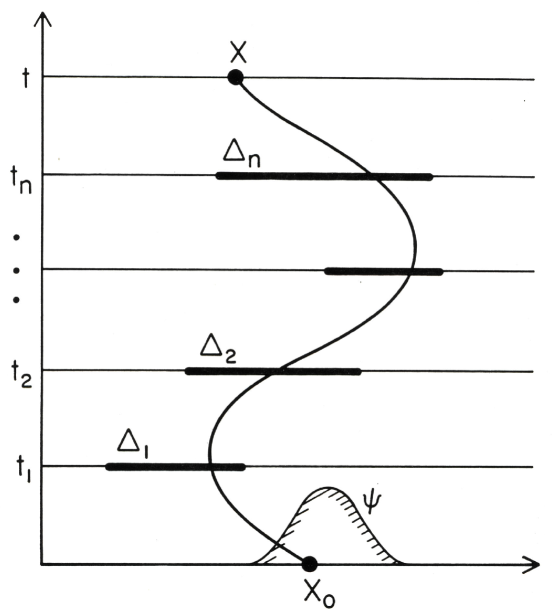
Figure 14: The semiclassical approximation to the quantum mechanics of a non-relativistic particle. Suppose at time $t=0$ the particle is in a state described is a wave function $\psi(q_{0})$. Its subsequent evolution exhibits classical correlations in time if successive determinations of position are correlated according to classical laws, that is, if the amplitude for non-classically correlated positions is near zero. The existence of such classical correlations is, therefore, a property not only of the initial condition but also the coarse graining used to analyze the subsequent motion. Classical correlations are properties of coarse-grained sets of histories of the particle. The amplitude for the particle to pass through intervals $\Delta_{1},\Delta_{2},\cdots,\Delta_{n}$ at times $t_{1},\cdots,t_{n}$ and arrive at $q_{f}$ at $t_{f}$ is the sum of exp ($iS$) over all paths to $q(t)$ that pass through the intervals, weighted by the initial wave function. For suitably spaced intervals in time, suitably large intervals $\Delta_{k}$, and suitable initial wave function $\psi$, this sum may be well approximated by the method of stationary phase. In that case, only when the intervals $\Delta_{k}$ are aligned about a classical path will there be a significant contribution to this sum. Classical correlations are thus recovered. How many classical paths contribute depends on the initial condition $\psi(q_{0})$. If, as illustrated here, it is a wave packet whose center follows a particular classical history then only that particular path will contribute significantly. By contrast, if $\psi$ is proportional to exp $[iS(q_{0})]$ for some classical action $S(q_{0})$, then all classical paths that satisfy $m\dot{q}=\partial S/\partial q$ will contribute. Then the prediction is of an ensemble of classical histories, each one correlated according to the classical equations of motion.

Classical correlations are predicted when the path integral in (406) can be done by the method of stationary phase. For then, only when $\Delta_{1},\cdots,\Delta_{n}$ are lined up so that a classical path from some $q_{0}$ to $q_{f}$ passes through them will the amplitude (406) be non-vanishing.

Whether a stationary phase approximation is appropriate for the path integral in (406) depends on the intervals $\Delta_{1},\cdots,\Delta_{n}$, the times $t_{1},\cdots,t_{n}$, and the initial wave function $\psi(q_{0})$. The $\Delta_{1},\cdots,\Delta_{n}$ must be large enough and the times $t_{1},\cdots,t_{n}$ separated enough to permit the destructive interference of the non-classical paths by which the stationary phase approximation operates. The $\Delta$’s must be small enough that a unique classical path passes through them. But, in addition to these requirements on the coarse graining, the initial $\psi(q_{0})$ must be right as well. There are a number of standard forms for $\psi(q_{0})$ for which the stationary phase approximation can be seen to be valid. For example, if $\psi(q_{0})$ describes a wave packet with position and momentum defined to an accuracy consistent with the uncertainty principle, and the time intervals between the $t_{k}$ are short compared with the time over which it spreads, and the $\Delta_{k}$ are greater than its initial width, then only a single path will contribute significantly to the integral — that classical path with the initial position and momentum of the wave packet. Another case leading to the validity of the stationary phase approximation is when $\psi(q_{0})$ corresponds to two initially separated wave packets. Then, two different classical paths contribute to the stationary phase approximation to (406) corresponding to the two sets of initial data. A unique classical trajectory is not predicted but rather one of two possible classical evolutions each with some probability determined by $\psi(q_{0})$.

In general, therefore, a detailed examination of the initial wave function $\psi(q_{0})$ is needed to determine if it predicts classical correlations in a suitably coarse-grained set of histories. However, there is a simple case when the requirements can be seen to be satisfied. This is when the Schrödinger evolution of the wave function $\psi(q_{0})$ is well approximated by forms like

$$\psi(q,t)\approx A(q,t)\ e^{\pm iS(q,t)/\hbar}$$ (407)

where $A(q,t)$ is a real slowly varying function of $q$ and $S/\hbar$ is a real, rapidly varying function of $q$. Eq. (407) thus separates $\psi(q_{0})\equiv\psi(q_{0},0)$ into a slowly varying prefactor and a rapidly varying exponential. It follows from the Schrödinger equation in these circumstances that $S$ is a classical action approximately satisfying the Hamilton-Jacobi equation

$$-\frac{\partial S}{\partial t}+H\left(\frac{\partial S}{\partial q},q\right)=0\,,$$ (408)

where $H$ is the Hamiltonian:

$$H=\frac{p^{2}}{2M}+V(q)\,.$$ (409)

The form (407) is general enough to include the familiar WKB case when $\psi(q,t)$ is an energy eigenfunction and $S(q)$ and $A(q)$ are independent of time with $S(q)$ satisfying $H(\partial S/\partial q,q)=E$.

The forms (407) are called semiclassical approximations. When the semiclassical approximation (407) is inserted in (406), the functional integral over paths $q(t)$ and the integral over $q_{0}$ are integrals of a slowly varying prefactor times a rapidly varying exponential. This is immediately of the form for which the stationary phase approximation will be valid for suitably large intervals $\Delta_{1},\cdots,\Delta_{n}$ and times $t_{1},\ \cdots,\ t_{n}$. The exponent of the integral is

$$S\big{[}q(\tau);q_{f},q_{0}\big{)}+S(q_{0},0)\,.$$ (410)

Here, $S[q(\tau);q_{f},q_{0})$ is the action functional for paths between $q_{0}$ and $q_{f}$ while $S(q_{0},0)$ is the classical action function specifying the initial semiclassical wave function. Extremization of the exponent (410) with respect to the paths $q(t)$ and the value of $q_{0}$ give the values that dominate the integral (406). Extremizing with respect to $q(t)$ keeping $q_{0}$ and $q_{f}$ fixed means the dominant paths satisfy the classical equations of motion. Extremizing with respect to $q_{0}$ gives the initial momentum of a path in terms of $S(q_{0},0)$:

$$p_{0}=\partial S/\partial q_{0}\,.$$ (411)

Like the two wave packet example above, a unique classical trajectory is not predicted. The wave function (407) is not peaked about some particular initial data. In fact, since $A(q_{0},0)$ varies slowly, it treats many $q_{0}$’s equally. Thus, for suitable subsequent intervals $\Delta_{k}$ and times, $t_{1},\cdots,t_{n}$ a semiclassical wave function predicts not just one classical trajectory, nor all of them, but just those for which the initial coordinates and momenta are related by (411) for the particular classical action $S$ defined by the initial wave function. A wave function of semiclassical form thus predicts an ensemble of classical trajectories, each differing from the other by the constant needed to integrate (411).

The prefactor $A$ is also of significance. Its square, $|A(q_{0},0)|^{2}$, is the probability of an initial $q_{0}$. Given that subsequent values of $q$ are correlated by the classical trajectory with this initial $q_{0}$ and the initial momentum (411), $|A(q_{0},0)|^{2}$ may be thought of as the probability of a particular classical trajectory crossing the surface $t=0$. The order $\hbar$ implication of the Schrödinger equation is that

$$\frac{\partial|A|^{2}}{\partial t}+\vec{\bigtriangledown}\ .\left(|A|^{2}\frac{\vec{\bigtriangledown}S}{M}\right)=0$$ (412)

so that the probability density $|A|^{2}$ is conserved along the trajectories.

IX.3 The Semiclassical Approximation for the Relativistic Particle

The argument that wave functions of semiclassical form imply classical correlations in time for suitably coarse-grained sets of histories extends straightforwardly from non-relativistic quantum mechanics to the quantum mechanics of spacetime. As a warm-up for the latter problem, however, we begin by considering a system with a single reparametrization invariance, specifically the free relativistic world line in flat spacetime with paths that move forward and backward in time. The generalized quantum mechanics for this system was developed in Section VII.

We suppose that the initial condition for the relativistic particle is supplied by a pure state whose Klein-Gordon wave function $\psi(x)$ is well approximated, in some region of spacetime, by the semiclassical form

$$\psi(x)\approx A(x)e^{iS(x)/\hbar}$$ (413)

where $A(x)$ is a slowly varying prefactor while the exponential varies rapidly. In this approximation, the most rapidly varying part of the Klein-Gordon equation implies the Hamilton-Jacobi equation for $S(x)$:

$$\left(\nabla S\right)^{2}+m^{2}=0\,,$$ (414)

which shows that $S(x)$ is a classical action. The conservation of Klein-Gordon current in this approximation of rapid variation of $S$ gives

$$\nabla\cdot\bigl{(}\bigl{|}A\bigr{|}^{2}\nabla S\bigr{)}=0\,,$$ (415)

which shows that $|A|^{2}$ is conserved along the integral curves of the classical action $S(x)$.

Unlike the case of non-relativistic quantum mechanics, the wave function $\psi(x)$ does not have a direct probability interpretation in the generalized quantum mechanics developed in Section VII. Rather, it supplies the initial condition for the decoherence functional from which the probabilities for decoherent partitions of the particle’s paths are determined. Despite this, we shall see that probabilities for those coarse grainings that define sets of histories that behave semiclassically can be extracted simply from the form of (413).

We consider a coarse graining of the paths of the relativistic particle into classes $c_{\alpha}$ that distinguish classical from non-classical behavior. An example would be coarse graining the paths $x(\lambda)$ by their behavior with respect to a division of spacetime into cells. Classical paths will go only through certain sequences of cells consistent with obeying the classical equation of motion. In the case of a free relativistic particle, the classical paths go through cells connected by straight lines in spacetime intersecting each cell once and only once. Non-classical paths connect cells in other ways.

We assume the decoherence of such a coarse-grained set of histories, $\{c_{\alpha}\}$, either by themselves or through interaction with a larger system as in a measurement situation. The relevant class operator matrix element for a particular coarse-grained history $c_{\alpha}$ is [cf. VII.4.19)]

$$\langle x^{\prime\prime}\|C_{\alpha}|\psi\rangle=i\int\nolimits_{\sigma^{\prime}}d\Sigma^{\nu}\left\langle x^{\prime\prime}\left\|C_{\alpha}\right\|x^{\prime}\right\rangle{\buildrel\leftrightarrow\over{\nabla^{\prime}}}_{\nu}\psi\left(x^{\prime}\right)$$ (416)

where the matrix elements of the class operator are defined by the path integral (274) and the integral is taken over a spacelike surface $\sigma^{\prime}$ to the past of any restriction by the coarse graining.

We further suppose, as a consequence of the semiclassical form (413) and the nature of the coarse grainings, that the integral over $x^{\prime}$ and the path integral defining the matrix elements of $C_{\alpha}$ can be done by the method of stationary phase. Inserting (413) in (416), using the gauge $\dot{N}=0$ in (276), we find an integral that is proportional to an exponential of the following combination:

$$S\left[x(\lambda),N;x^{\prime\prime},x^{\prime}\right)+S\left(x^{\prime}\right)$$ (417)

where we have indicated the dependence of the action on the endpoints explicitly. In the stationary phase approximation, only paths that extremize this combination with respect to the variables integrated over in (416) contribute to the integral. Extremization with respect to $x(\lambda)$ and $N$ yield the classical equations of motion. The variable $x^{\prime}$ is to be extremized in the surface $\sigma^{\prime}$ in which it is integrated. This gives the connection between the components of the momentum of the classical path in the surface and the tangential derivatives of $S(x)$. The remaining component is determined by the constraint (414) and we can therefore write initially

$$p^{\prime}=\nabla_{x^{\prime}}S\,.$$ (418)

Thus, with these assumptions, a wave function of the semiclassical form (413) predicts that suitable coarse grainings will define an ensemble of histories correlated in time by the classical equations of motion having any of the possible initial positions on the initial surface $\sigma^{\prime}$ with an initial momentum determined (418). To calculate the probability of a particular history we only have to calculate the probability of the position that it crosses $\sigma^{\prime}$. These are determined by the diagonal elements of the decoherence functional (318).

For simplicity, let us, assume that the surfaces $\sigma^{\prime}$ and $\sigma^{\prime\prime}$ are surfaces of constant time, $t^{\prime}$ and $t^{\prime\prime}$ respectively. We calculate the probability that the classical path passes through a particular spatial region $\alpha$ of the surface $\sigma^{\prime}$ having volume $\Delta_{\alpha}$ centered about position ${\bf x}_{\alpha}$. According to (318) this is

$$p(\alpha)={\cal N}\int\frac{d^{3}p^{\prime\prime}}{(2\pi\hbar)^{3}2\omega_{p^{\prime\prime}}}\left|\left\langle\phi_{{\bf p}^{\prime\prime}}\right|C_{\alpha}\left|\psi\right\rangle\right|^{2}.$$ (419)

Here, we have assumed a final condition of indifference with respect to final states implemented by a sum over a complete set of positive frequency momentum eigenstates having Klein-Gordon wave functions

$$\phi_{\bf p}(x)=\hbar^{\textstyle{1\over 2}}\exp\left[i\left(-\omega_{p}t+{\bf p}\cdot{\bf x}\right)\right/\hbar]$$ (420)

where, as usual, $\omega_{p}=\sqrt{{\bf p}^{~{}2}+m^{2}}$. The matrix elements of $C_{\alpha}$ are

$$\left\langle\phi_{{\bf p}^{~{}\prime\prime}}\left|C_{\alpha}\right|\psi\right\rangle=-\int_{{\bf R}^{3}}d^{3}x^{\prime\prime}\int_{\alpha}d^{3}x^{\prime}\ \phi^{*}_{{\bf p}^{~{}\prime\prime}}(x^{\prime\prime})\frac{\buildrel\leftrightarrow\over{\partial}}{\partial t^{\prime\prime}}\Delta_{F}\left(x^{\prime\prime}-x^{\prime}\right)\frac{\buildrel\leftrightarrow\over{\partial}}{\partial t^{\prime}}\psi(x^{\prime})\,.$$ (421)

Noting that

$$\rho_{f}\left(x^{\prime\prime},x^{\prime}\right)\equiv\int\frac{d^{3}p}{(2\pi\hbar)^{3}2\omega_{p}}\,\phi_{\bf p}\left(x^{\prime\prime}\right)\,\phi^{*}_{\bf p}\left(x^{\prime}\right)=-i\Delta_{F}\left(x^{\prime\prime}-x^{\prime}\right)\,,$$ (422)

and composing Feynman propagators where appropriate, we can write for the probability (419)

$$p(\alpha)={\cal N}\int_{\alpha}d^{3}x^{\prime\prime}\int_{\alpha}d^{3}x^{\prime}\ \psi^{*}\left(x^{\prime\prime}\right)\ \frac{\buildrel\leftrightarrow\over{\partial}}{\partial t^{\prime\prime}}\Delta_{F}\left(x^{\prime\prime}-x^{\prime}\right)\ \frac{\buildrel\leftrightarrow\over{\partial}}{\partial t^{\prime}}\psi\left(x^{\prime}\right)$$ (423)

where $x^{\prime\prime}$ and $x^{\prime}$ both lie on the constant time spacelike surface $\sigma^{\prime}$. This can be evaluated as follows: Insert the semiclassical form (413) in (423) and note that the slowly varying prefactor $A(x)$ can be pulled outside all integrations and evaluated at the center ${\bf x}_{\alpha}$ of the interval $\Delta_{\alpha}$. To evaluate the remainder of the integral insert the standard integral representation for $\Delta_{F}$ following from (422) and (420) into (423). Note that, if the characteristic size of the region $\Delta_{\alpha}$ is large compared to the Compton wave length $\hbar/m$, the various factors of $\omega_{p}$ may be replaced by $(\partial S/\partial t^{\prime})$, when the latter is positive like $\omega_{p}$, because the integrations over ${\bf x}^{\prime\prime}$ and ${\bf x}^{\prime}$ approximately enforce the connection (418). If $\partial S/\partial t^{\prime}$ is negative the integral is zero in these approximations. Carrying out the remaining integrations one finds

$$p(\alpha)={\cal N}\left|A\left(t^{\prime},{\bf x}_{\alpha}\right)\right|^{2}\Delta_{\alpha}\,\theta\left(\partial S/\partial t^{\prime}\right)\,\partial\left[S\left(t^{\prime},{\bf x}_{\alpha}\right)/\hbar\right]/\partial t^{\prime}\,.$$ (424)

The normalization factor, ${\cal N}$ can be determined in this approximation by requiring the probabilities to be normalized, $\Sigma_{\alpha}p(\alpha)=1$.

The restriction to coarse grainings that distinguish classical paths only up to errors in position larger than the Compton wavelength may be understood in another way. The exact notion of localization for the relativistic particle is provided by the Newton-Wigner position operator NW49 . A state localized in the Newton-Wigner sense does not have a localized Klein-Gordon wave function, rather one spread out over coordinate intervals of order $\hbar/m$. Throughout, we have been discussing coarse grainings defined in terms of the coordinates of spacetime by which the fine-grained histories are defined. We should, therefore, not expect to obtain a notion of classical position that is defined more accurately than the Compton wavelength. We do not.

The result (424) is not a surprise. The conservation of Klein-Gordon current leads to the conservation of $|A|^{2}\nabla S$ in the semiclassical approximation [cf. (415)]. In view of the connection (418) between $\nabla S$ and four-velocity, this can be interpreted as the conservation of the density $|A|^{2}$ along classical trajectories. We, therefore, naturally are led to think of

$$|A|^{2}\nabla_{\mu}Sd\Sigma^{\mu}\,,$$ (425)

when positive, as the relative probability that the classical trajectories cross an element of spacelike hypersurface $d\Sigma^{\mu}$. This is the rule that was advocated by many authors for a probability interpretation of semiclassical wave functions of reparametrization invariant systems especially clearly and completely by Vilenkin Vil88 . Here, we have derived this rule from a more fundamental probability interpretation through which the limitations of the approximation can be explored.

It should be stressed that we have exhibited no readily applicable rule for determining which coarse grainings lead to classical correlations. For example, we expect the semiclassical approximation (413) to be valid only in some region of spacetime. Coarse grainings that distinguish between paths outside this region cannot be expected to exhibit classical correlations. In particular, in evaluating the integral over $x^{\prime}$ that led to (418) we, in effect, assumed that the semiclassical form (413) was valid over the whole of the surface $\sigma^{\prime}$. If that is not true a more delicate argument with possibly more stringent requirements on the coarse graining may be needed to exhibit classical correlations in time. The important point is that the generalized quantum mechanics for a single relativistic particle gives us a precise meaning for the probabilities of decoherent sets of coarse-grained histories in which various approximation schemes can be analyzed and their limitations explored.

IX.4 The Approximation of Field Theory in Semiclassical Spacetime

Any generalization of quantum mechanics that is proposed to deal with the problem of time in quantum gravity must reproduce the usual Hamiltonian quantum mechanics of matter fields in a fixed background spacetime for those coarse-grained histories in which spacetime geometry behaves classically. To discuss this question, a more refined type of semiclassical approximation is needed than the kind we have discussed for non-relativistic systems or the relativistic particle. In these, all variables behave classically. To discuss the recovery of quantum field theory in classical spacetime we need to treat the matter field variables fully quantum mechanically in situations where geometry behaves approximately classically. Such approximations are familiar from other areas of physics. In the Born-Oppenheimer approximation to molecular dynamics, for example, the motion of the nuclei is treated classically while the dynamics of the electrons is treated quantum mechanically.

In ordinary quantum mechanics, wave functions that are products of a rapidly oscillating function of semiclassical form like (407) in some variables times a more slowly varying function of the remaining ones lead to classical behavior of the former and quantum behavior of the latter. Typically there is a scale that governs the separation into rapidly and slowly varying parts. In the case of the Born-Oppenheimer approximation it is the ratio of the mass of the nuclei to that of the electron. The ratio of the Planck mass to characteristic particle energies will be the important ratio in approximations where spacetime geometry behaves classically but matter behaves quantum mechanically.

The initial condition for cosmology is represented by wave function(s) on superspace that solve operator versions of the constraints. Procedures for constructing wave functions of various semiclassical forms that approximately satisfy the constraints have been widely discussed in the literature and we shall only briefly review them here. For details and references to the original literature the reader can consult the papers of Halliwell Hal87 and Padmanabhan and Singh PS90 . Many different semiclassical forms are possible depending on what variables the rapidly and slowly varying parts of the wave function depend on. To illustrate with a simple case we consider wave functions of the form

$$\Psi\left[h_{ij}({\bf x}),\chi({\bf x})\right]=A[h_{ij}({\bf x})]\exp(\pm iS_{0}[h_{ij}({\bf x})])\psi\left[h_{ij}({\bf x}),\chi({\bf x})\right]\,,$$ (426)

where $A$ and $\psi$ are slowly varying functionals of $h_{ij}({\bf x})$ and $S_{0}[h_{ij}({\bf x})]$ is a real classical action for gravity alone and we have reverted to units where $\hbar=1$ for the remainder of this section. The action $S_{0}[h_{ij}({\bf x})]$ satisfies the classical Hamilton-Jacobi equations Per62 ; Ger69 that arise from the constraints of general relativity $H(\pi^{ij},h_{ij})=0$ and $H_{i}(\pi^{ij},h_{ij})=0$ when the momentum $\pi^{ij}({\bf x})$ conjugate to $h_{ij}({\bf x})$ is related to $S_{0}$ by

$$\pi^{ij}({\bf x})=\frac{\delta S_{0}}{\delta h_{ij}({\bf x})}\,.$$ (427)

Explicitly [cf. (VIII.4.8)] these constraints are:

$$\ell^{2}G_{ijk\ell}({\bf x})\pi^{ij}({\bf x})\pi^{k\ell}({\bf x})+\ell^{-2}h^{{\textstyle{1\over 2}}}({\bf x})\left(2\Lambda-^{3}R({\bf x})\right)=0\,.$$ (428a)

$$D_{j}\pi^{ij}({\bf x})=0\,.$$ (428b)

The gradient (427) defines a vector field on superspace and its integral curves are the classical spacetimes that give rise to the action $S_{0}$. For example, if we work in the gauge where four-metrics have the form

$$ds^{2}=-d\tau^{2}+h_{ij}(\tau,{\bf x})dx^{i}dx^{j}\,,$$ (429)

then eq. (427) becomes

$${\textstyle{1\over 2}}\frac{dh_{ij}}{d\tau}=G_{ijk\ell}\frac{\delta S_{0}}{\delta h_{k\ell}}\,.$$ (430)

Integrating (430), we recover a four-metric (429) that satisfies the Einstein equation. The values of $\psi$ along such an integral curve define $\psi$ as a function of $\tau$

$$\psi=\psi\left[h_{ij}(\tau,{\bf x}),\chi({\bf x})\right]=\psi\left[\tau,\chi({\bf x})\right]\,.$$ (431)

The wave function $\Psi[h_{ij}({\bf x}),\chi({\bf x})]$ must satisfy the operator form of the constraints (371) that implement the underlying gravitational dynamics. The three momentum constraints, ${\cal H}_{i}\Psi=0$, guarantee that $\Psi$ is independent of the choice of coordinates in the spacelike surface. The Hamiltonian constraint may be written out formally as

$${\cal H}_{0}({\bf x})\Psi=\left[-\ell^{2}\nabla^{2}_{\bf x}+\ell^{-2}h^{{\textstyle{1\over 2}}}(2\Lambda-^{3}R)+h^{{\textstyle{1\over 2}}}\hat{T}_{nn}(\chi,-i\delta/\delta\chi)\right]\Psi=0\,.$$ (432)

Here,

$$\nabla^{2}_{\bf x}=G_{ijk\ell}({\bf x})\frac{\delta^{2}}{\delta h_{ij}({\bf x})\delta h_{k\ell}({\bf x})}+\left(\begin{array}[]{l}{\rm linear\ derivative}\\ {\rm terms\ depending}\\ {\rm on\ factor\ ordering}\end{array}\right)$$ (433)

and $\hat{T}_{nn}$ is the stress-energy of the matter field projected into the spacelike surface (the Hamiltonian density) expressed as a function of the matter field $\chi({\bf x})$ and the operator $-i\delta/\delta\chi({\bf x})$ corresponding to its conjugate momentum. This operator form of the Hamiltonian constraint is called the Wheeler-DeWitt equation DeW67 ; Whe68 . The implications of the Wheeler-DeWitt equation (432) for that part of the semiclassical approximation that varies slowly with three-metric may be found by inserting the approximation (426) into (432), using the Hamilton-Jacobi equation (428), and neglecting second derivatives of terms varying slowly with respect to the three-metric. The result is an equation for $A\psi$ that can be organized in the following form:

$$-i\psi\left[(\nabla^{2}_{\bf x}S_{0})A+2G_{ijk\ell}\frac{\delta S_{0}}{\delta h_{ij}}\frac{\delta A}{\delta h_{k\ell}}\right]+A\left[-2iG_{ijk\ell}\frac{\delta S_{0}}{\delta h_{ij}}\frac{\delta\psi}{\delta h_{k\ell}}+\ell^{-2}h^{\textstyle{1\over 2}}\hat{T}_{nn}\psi\right]=0\,.$$ (434)

We now impose the condition that the two terms in (434) vanish separately. This defines a decomposition of the slowly varying part, $A\psi$, into $A$ and $\psi$.

The condition on the $\psi$ resulting from (434) may be rewritten using (430) and (432) as

$$i\frac{\partial\psi}{\partial\tau}=h^{\textstyle{1\over 2}}\hat{T}_{nn}\left(\chi,-i\frac{\delta}{\delta\chi}\right)\psi\,.$$ (435)

This is the Schrödinger equation in the field representation for a quantum matter field $\chi$ executing dynamics in a background geometry of the form (429).

The condition on $A$ arising from (434) implies the following relation

$$G_{ijk\ell}\frac{\delta}{\delta h_{ij}}\left(|A|^{2}\frac{\delta S_{0}}{\delta h_{k\ell}}\right)=0\,.$$ (436)

This is the equation of conservation of the current $|A|^{2}(\delta S_{0}/\delta h_{ij})$ in superspace. It is the analog of the similar relation (412) in non-relativistic quantum mechanics and (415) in the quantum mechanics of the relativistic particle. Indeed, in view of (430), this is just the statement that the “density in superspace”, $|A|^{2}$, is conserved along classical trajectories, the integral curves of (430).

Many other semiclassical approximations are possible besides the one based on the form (413). For example, an approximate form in which both spacetime and some matter variables behave classically would involve an action defining the rapidly varying part of the wave function which depended on both kinds of variables. One can consider ensembles of classical geometries driven by expectation values of matter fields in which the constraints (428) contain such terms as sources. Systematic approaches to obtaining such approximate wave functions by expanding the solutions to the Wheeler-DeWitt equation in powers of the inverse Planck length have been extensively discussed. Indeed, it is essential to consider approximations with both matter and geometry behaving classically since the late universe is certainly not a solution of the vacuum Einstein equation. Superpositions of semiclassical forms like those of (426), such as those which arise from the “no boundary” proposal of the initial condition HH83 , may also be considered. Provided that there is no interference between the branches arising from distinct semiclassical forms, the probability of a coarse-grained history is just the sum of contributions from each. The common feature of all these semiclassical approximations is the separation of the wave function into superposition of pieces each having a part rapidly varying in certain variables governed by a classical action and a more slowly varying part. There are different approximations depending on what variables are distinguished in this way.

We now sketch a derivation of how an initial condition of the form (426) can imply the classical behavior of geometry in suitable coarse grainings and the familiar quantum mechanics of matter fields in the resulting background classical spacetimes. We shall give only the broad outlines of a demonstration making many assumptions that must be made precise and justified to complete it.

We assume that we have a coarse graining of geometry that distinguishes classical from non-classical behavior. That is, we assume that the four-dimensional metrics that are the fine-grained histories of geometry are partitioned into classes $\{c_{\alpha}\}$ such that some of the classes can be said to exhibit the classical correlations implied by Einstein’s equation to a sufficient accuracy while the rest do not. We let the index $\gamma$ range over the subset of the $\alpha$ corresponding to possible classical histories so that $\{c_{\gamma}\}$ is the set of possible coarse-grained classical histories. Each of the classes $c_{\gamma}$ may be further partitioned by the behavior of the matter field into a finer set of classes $\{c_{\gamma\beta}\}$. The classes $c_{\gamma\beta}$ of physical interest will typically be highly branch dependent as described in Section III.1.1, that is, the partitions of the matter field of interest will depend on the classical spacetime geometry $\gamma$. We thus have a division of the fine-grained histories into non-classical geometries and various classical geometries with different behaviors for the matter field in those classical spacetimes. We denote the coarse-grained classes by $\{c_{\alpha\beta}\}$ understanding that for the non-classical alternatives for the geometry there is but a single alternative $\beta$ for the matter — all possible field histories. Our central assumption is that the geometrical alternatives decohere, that is that the decoherence functional is approximately diagonal in the alternatives $\alpha$ (which include the alternative classical histories, $\gamma$).

The decoherence functional (385) is constructed from amplitudes of the form

$$\left\langle h^{\prime\prime},\chi^{\prime\prime}\left\|C_{\alpha\beta}\right\|h^{\prime},\chi^{\prime}\right\rangle\circ\Psi\left[h^{\prime},\chi^{\prime}\right]$$ (437)

where we are using a compressed notation in which indices (including coordinate labels) have been suppressed. The class operator matrix elements are [cf. (382)]

$$\left\langle h^{\prime\prime},\chi^{\prime\prime}\left\|C_{\alpha\beta}\right\|h^{\prime},\chi^{\prime}\right\rangle=\int_{\alpha\beta}\delta g\delta\phi\,\Delta_{\Phi}[g,\phi]\delta[\Phi[g,\phi]]\exp\left\{i\left(S_{E}[g]+S_{M}[g,\phi]\right)\right\}\,.$$ (438)

Including the integral over $h^{\prime}$ and $\chi^{\prime}$ involved in the $\circ$ product, the amplitude (437) is defined by a functional integral over metrics and matter fields including their values on the initial surface $\sigma^{\prime}$. We now assume that the coarse graining is such that, for wave functions of the semiclassical form (426), the integral over metrics can be carried out by the method of stationary phase. Significant contributions come only from the extrema of the exponent

$$S_{E}\left[g;h^{\prime\prime},h^{\prime}\right]+S_{0}\left[h^{\prime}\right]$$ (439)

with respect to $g$ and $h^{\prime}$. Eq. (439) is extremized with respect to $g$ by solutions of the Einstein equations with no matter sources. Eq. (439) is an extremum with respect to $h^{\prime}$ when the initial momenta of these classical solutions is connected to $S_{0}$ by the classical relation (427). In this approximation, therefore, amplitude for non-classical behavior of the geometry is zero; classical spacetime is predicted.

We assume that the coarse graining defining the classical classes $\{c_{\gamma\beta}\}$ is fine enough that an essentially unique geometry (up to the accuracy of the coarse graining) provides the extremum between $\sigma^{\prime\prime}$ and $\sigma^{\prime}$ and dominate the sum over metrics in the corresponding amplitudes (437). Denote by $g_{\gamma}$ a metric representing this solution of the Einstein equation that satisfies the gauge conditions $\Phi^{\alpha}[g]=0$. Denote by $\sigma^{\prime\prime}_{\gamma}$ and $\sigma^{\prime}_{\gamma}$ respectively the hypersurfaces in the classical spacetime that respectively correspond to the surfaces $\sigma^{\prime\prime}$ and $\sigma^{\prime}$ in superspace. Taking account of the semiclassical form (426), the amplitude (437) may be written

$$A_{\gamma}F_{\gamma}\int\delta\chi^{\prime}\left\langle\chi^{\prime\prime},\sigma^{\prime\prime}_{\gamma}\left\|C_{\gamma\beta}\right\|\chi^{\prime},\sigma^{\prime}_{\gamma}\right\rangle\,\psi\left[\chi^{\prime},\sigma^{\prime}_{\gamma}\right]\,.$$ (440)

where

$$\left\langle\chi^{\prime\prime},\sigma^{\prime\prime}_{\gamma}\left\|C_{\gamma\beta}\right\|\chi^{\prime},\sigma^{\prime}_{\gamma}\right\rangle=\int_{\gamma\beta}\delta\phi\,\exp\left(iS_{M}\left[g_{\gamma},\phi\right]\right)\,.$$ (441)

These expressions were arrived at as follows: The slowly varying factor $A[h_{ij}]$ in (426) was evaluated at the value of $h_{ij}$ corresponding to the classical solution $g_{\gamma}$, pulled out of the integral and written $A_{\gamma}$. The functional integral over fields in the class $c_{\gamma\beta}$ occurs in (441). It is an integral over all fields that are in the class $c_{\gamma\beta}$ and match the values $\chi^{\prime}$ and $\chi^{\prime\prime}$ on the hypersurfaces $\sigma^{\prime}_{\gamma}$ and $\sigma^{\prime\prime}_{\gamma}$ respectively. The remaining factors arising from the stationary phase approximation to the integral over metrics are lumped together in $F_{\gamma}$.

Assuming that measure induced from (380) has an appropriate form, the matrix elements (441) define the class operators of a matter field theory in the background spacetime $g_{\gamma}$. The composition with the wave function $\psi[\chi^{\prime},\sigma^{\prime}_{\gamma}]$ is the usual inner product between states of definite field on a hypersurface $\sigma^{\prime}_{\gamma}$. Now assume that the wave functions $\{\Phi_{i}(h^{\prime\prime},\chi^{\prime\prime})\}$ specifying the final condition factor into products of functions of $h^{\prime\prime}$ and functions of $\chi^{\prime\prime}$. When we construct the full decoherence functional from the amplitudes (440) we find for the only non-vanishing values

$$D\left(\gamma^{\prime},\beta^{\prime};\gamma,\beta\right)\cong\delta_{\gamma^{\prime}\gamma}\left|A_{\gamma}\right|^{2}{\cal F}_{\gamma}D^{M}_{\gamma}\left(\beta^{\prime},\beta\right)$$ (442)

where $D^{M}_{\gamma}\left(\beta^{\prime},\beta\right)$ is the decoherence functional for matter field alternatives $\{c_{\gamma\beta}\}$ in the fixed background spacetime $g_{\gamma}$. The factor ${\cal F}_{\gamma}$ represents the combination of the factors $F_{\gamma}$ and the final conditions on geometry.

Eq. (442) shows the sense in which the generalized quantum mechanics of spacetime and matter fields reproduces field theory in curved spacetime when the geometry behaves classically. The decoherence and probabilities of matter alternatives are governed by the field theory in curved spacetime decoherence functional $D^{M}_{\gamma}(\beta^{\prime},\beta)$ in each classical spacetime $g_{\gamma}$. The probabilities of the different possible classical geometries themselves are given by $|A_{\gamma}|^{2}{\cal F}_{\gamma}$. The conservation of current (436) makes it plausible that with suitable final conditions ${\cal F}_{\gamma}$ will be the “velocity” $\delta S_{0}/\delta h_{ij}$. However, a more careful analysis of the final conditions and the stationary phase approximation would be needed to conclude such a result.

IX.5 Rules for Semiclassical Prediction and the Emergence of Time

While not complete, the discussion in this section points to two conclusions: First, the usual rules for extracting the semiclassical predictions of a wave function of the universe can be made precise and justified in the generalized sum-over-histories quantum mechanics of cosmological spacetimes. A wave function specifying an initial condition does not generally have a direct probability interpretation in this framework. It is an input to the calculation of the probabilities of partitions of cosmological four-geometries and matter field configurations into decoherent classes. However, wave functions of the semiclassical form (426) imply that suitably coarse-grained, decoherent sets of histories will, with high probability, exhibit the correlations of classical spacetime. For each initial three-metric there is such a classical spacetime. It can be found by integrating the Einstein equation with the initial data

$$h_{ij}({\bf x}),\,\,\,\,\pi^{ij}({\bf x})=\delta S_{0}/\delta h_{ij}({\bf x})\,.$$ (443)

Thus, an initial condition represented by a wave function that is approximately of the semiclassical form (426) may be said to predict the ensemble of classical spacetimes with the initial data of (443). Not all classical spacetimes are predicted for that would correspond to all data $(h_{ij},\pi^{ij})$ consistent with the constraints. Rather, only classical spacetimes corresponding to the initial data of the particular form of the initial wave function through (443) are predicted. The relative probabilities of these classical spacetimes are proportional to $|A[h_{ij}]|^{2}$ as (442) shows.

The utility of a general framework for prediction is not simply to justify the rules for semiclassical prediction that were posited on the basis of analogy with non-relativistic quantum mechanics. The more general framework allows us to analyze the deviations from these rules. It permits classical behavior to be precisely defined in terms of the probabilities for histories. It permits an analysis of what level of coarse graining is necessary for a classical description. It allows us to understand quantitatively how close the initial wave function has to come to a semiclassical form to predict classical histories. It allows us to calculate the probabilities for deviations from classical behavior and to analyze when the semiclassical rules break down. It permits the calculation of probabilities for highly non-classical alternatives. Most importantly, it allows us to analyze which sets of alternative coarse-grained sets of histories of the universe decohere.

The second conclusion which the discussion of this section points to concerns the problem of time in quantum gravity. The sum-over-histories generalized quantum mechanics we have been describing is in fully four-dimensional form and does not require the specification of a preferred family of spacelike surfaces. Yet we have seen in eq. (442) how for coarse grainings that exhibit the correlations of classical geometry, the decoherence functional can reduce to the decoherence functional $D^{M}_{\gamma}(\beta^{\prime},\beta)$ for field theory in a curved spacetime, $g_{\gamma}$. That theory does have an equivalent Hamiltonian formulation in terms of states on any family of spacelike surfaces that foliate the background spacetime, $g_{\gamma}$. Its construction follows the discussion in Section IV.4. Assuming that the measure induced from the Liouville construction in (380) is appropriate, the resulting states evolve unitarily when unrestricted by the coarse graining. States and unitarity may thus be recovered in quantum theory, not generally, but in approximations in which spacetime geometry behaves classically. The consistency of Hamiltonian formulation on different foliating families of spacelike surfaces is guaranteed by their equivalence with the sum-over-histories formulation and traceable ultimately to the causal structure supplied by the background geometry $g_{\gamma}$.

For example, let us consider how the time ordering of the alternatives in the class operators of Hamiltonian quantum mechanics [cf. (14)] emerges from the generalized quantum mechanics of spacetime which has no preferred time and therefore a fortiori no notion of time ordering. Making essential use of the possibility of branch dependent partitions, consider a coarse graining of the matter field histories by ranges of field averages over spatial regions on a succession of non-intersecting spacelike surfaces $\sigma_{\gamma 1},\cdots,\sigma_{\gamma n}$ of the background geometry $g_{\gamma}$. The class operators defined by (441) will be given by matrix elements of projection operators that are time-ordered with respect to the causal structure of the background geometry. That is because functional integrals defining matrix elements of products of operators automatically time-order them [cf. (176)]. Arrows of time, such as the second law of thermodynamics, then can arise from asymmetries between the initial and final conditions on the matter fields as described in Section IV.7. It is in such ways that a preferred notion of time enters quantum mechanics when there is a classical background spacetime to supply it.

X Summation

These lectures have developed generalized quantum frameworks for non-relativistic quantum mechanics, field theory, and a single relativistic world line in which quantum theory is put into fully spacetime form both with respect to dynamics and alternatives. These frameworks motivate the proposal of Section VIII for a quantum framework for cosmology incorporating a quantum dynamics of spacetime geometry. The three basic elements of a generalized quantum theory are compared for these frameworks in the table above.

• Quantum mechanics is formulated for a closed system — the universe. Decoherence rather than measurement distinguishes those alternatives which may consistently be assigned probabilities from those which may not. The framework may thus be applied to make predictions of alternatives of interest to cosmology in the very early universe or on very large distance scales which are not part of any measurement situation.

• The sum-over-histories approach to quantum mechanics is used to formulate the quantum mechanics of cosmology in fully spacetime form. Dynamics is expressed in terms of sums over fine-grained histories that are four-dimensional manifolds, metrics, and matter field configurations. Alternatives are defined by partitions (coarse-grainings) of these four-dimensional, fine-grained histories into exhaustive sets of exclusive diffeomorphism invariant classes. The analogs of “unitary evolution” and “reduction of the wave packet” are given a unified sum-over-histories expression. The formulation is manifestly four-dimensionally diffeomorphism invariant.

• The alternatives to which this quantum theory assigns probabilities, if they decohere, are at once more general and more restricted than the “observables” that are often considered in other formulations. Four-dimensional diffeomorphism invariant alternatives on a spacelike surface, for example, usually are restricted to classical constants of the motion in the sense that they commute with the constraints. The present formulation considers the much larger, more realistic, and more accessible class of diffeomorphism invariant spacetime alternatives. However, in its present form the theory considers only alternatives describable in spacetime form as partitions of the unique fine-grained set of histories of the sum-over-histories formulation. Alternatives analogous to all the Hermitian observables of transformation theory are considered approximately by expressing them in spacetime form. A spacetime description is adequate for our experience and for cosmology. It remains to be seen whether it is fundamental, as assumed here, or whether the theory can be extended to an even richer class of alternatives.

• The generalized quantum mechanics of spacetime is free from the “problem of time”. No preferred family of spacelike surfaces was needed either to define the fine-grained histories or quantum evolution or the alternatives for which probabilities are predicted. These were specified directly in four-dimensional, geometrical, terms. This does not mean that the notion of time has been eliminated from this framework, for this is a quantum theory of spacetime! But this generalized quantum framework for spacetime neither requires nor specifies a preferred family of spacelike surfaces.

• Familiar Hamiltonian quantum mechanics of matter fields, with its preferred time(s), is an approximation to this generalized quantum mechanics of spacetime. The approximation is appropriate for decoherent coarse-grainings that specify coarse-grained geometries that are correlated classically with high probability. The classical geometries that summarize these correlations supply the notion of time for an approximate Hamiltonian quantum mechanics of matter fields. Such classical behavior of geometry is an emergent feature of the boundary conditions in cosmology. Having generalized Hamiltonian quantum mechanics to deal with quantum spacetime, we recover known physics in a suitable limit.

• A significant advantage of the sum-over-histories formulation of quantum mechanics is that the classical limit may be analyzed directly. That is especially important in quantum cosmology where we expect that most predictions of particular theories of the initial condition that can be confronted with observation will be semiclassical in nature. A system behaves classically when, in a suitably coarse-grained decoherent set of histories, the probability is high for histories correlated by deterministic laws. These probabilities are supplied by this generalized quantum framework. The wave function that specifies the initial condition does not have a direct probabilistic interpretation in this framework. However, assuming their decoherence, the probabilities for histories can be used to provide a justification for the familiar rules that have been used to extract semiclassical predictions directly from wave functions of semiclassical form.

• A lattice version of this generalized quantum mechanics can be constructed using the methods of the Regge calculus to consider fine-grained histories that are four-dimensional simplicial geometries. Such quantum models are a natural cut-off version of general relativity. They supply a finite and tractable arena in which to examine the low energy, large scale predictions of specific proposals for initial condition and with which to test the sensitivity of these predictions to the nature of quantum gravity at smaller scales.

• This sum-over-histories formulation of the quantum mechanics of cosmological spacetimes is a generalization of familiar quantum mechanics that neither utilizes states on spacelike surfaces nor even permits their construction in general. It is therefore different from the usual versions of Dirac or ADM quantum mechanics which are formulated in terms of states on a spacelike surface. Constraints do not play a primary role in constructing quantum dynamics. States satisfying the constraints are used to specify the initial and final conditions of a quantum cosmology but it is only in this sense that “true physical degrees of freedom” are defined. However, should a preferred time be discovered in classical general relativity nothing necessarily needs to be changed in this formulation of the quantum mechanics of spacetime as long as that preferred structure is expressible in terms of the metric. Further, should experiment show that quantum theory breaks general covariance by singling out a preferred family of spacelike surfaces not distinguished by the classical theory it is still possible to construct a generalized quantum mechanics on the principles described here, by suitably restricting the set of fine-grained histories.

This short list of attractive features does not mean that the generalized quantum mechanics of spacetime that we have described is correct. That determination is, in principle, a matter for experiment and observation. Of course, we are unlikely to have such experimental checks any time in the near future. As far as quantum cosmology is concerned, the main result of these investigations is to show that the rules for semiclassical prediction that are commonly employed can be put on a firmer probabilistic footing in a generalized quantum framework that does not require a preferred notion of time or or a definition of measurement.

Beyond theories of the initial condition, it is possible that these ideas may be useful in formulating a complete and manageable quantum theory of gravity which must necessarily predict the quantum behavior of spacetime geometry in a suitable limit. Thus, while we have learned little about a correct quantum theory of gravity in these lectures, we may have learned something of how to formulate questions to ask of it.

Notation and Conventions

For the most part we follow the conventions of Misner, Thorne, and Wheeler MTW70 with respect to signature, curvature, and indices. In particular:

Signature — $(-,+,+,+)$ for Lorentzian spacetimes.

Indices — Greek indices range over spacetime from 0 to 3. Latin indices range over space from 1 to 3. Indices on tensors are often suppressed where convenient.

Units — In Sections VI-VIII we use units in which $\hbar=c=1$. In Section IX we include $\hbar$ explicitly but set $c=1$; The length $\ell$ is $\ell=(16\pi G)^{\textstyle{1\over 2}}=1.15\times 10^{-32}$cm which is $(4\pi)^{\textstyle{1\over 2}}$ times the Planck length.

Coordinates and Momenta — The four coordinates of spacetime $\{x^{\alpha}\}$ are frequently abbreviated just as $x$. Similarly, conjugate momenta $\{p_{\alpha}\}$ are abbreviated as $p$. Spatial coordinates $\{x^{i}\}$ are written ${\bf x}$ and spatial momenta $\{p_{i}\}$ as ${\bf p}$. Thus $p\cdot x=p_{\alpha}x^{\alpha}$ and ${\bf p}\cdot{\bf x}=p_{i}x^{i}$. Similarly, configuration space coordinates $\{q^{i}\}$ are written as $q$, conjugate momenta $\{p_{i}\}$ as $p$, and $p\cdot q=p_{i}q^{i}$.

Vectors — Four-vectors $a^{\alpha},b^{\alpha},\cdots$ are written $a,b,c\cdots$ and their inner products as $a\cdot b$, etc. Three-vectors are written as $\vec{a},\vec{b},\vec{c}\cdots$ and their inner products as $\vec{a}\cdot\vec{b}$, etc. Thus, in the case of displacement vectors and their conjugate momenta we use ${\bf p}\cdot{\bf x}=\vec{p}\cdot\vec{x}$ interchangeably.

Covariant Derivatives — $\nabla_{\alpha}$ denotes a spacetime covariant derivative and $D_{i}$ a spatial one. $\nabla^{2}=\nabla_{\alpha}\nabla^{\alpha}$. In flat space $\nabla f$ is $\nabla_{\alpha}f$ and $\vec{\nabla}f$ is the usual three-dimensional gradient.

Traces and Determinants — Traces of second rank tensors $K_{\alpha\beta}$ are written as $K=K^{\alpha}_{\alpha}$ except when the tensor is the metric in which case $g$ is the determinant of $g_{\alpha\beta}$ and $h$ the determinant of spatial metric $h_{ij}$;

Extrinsic Curvatures — If $n_{\alpha}$ is the unit normal to a spacelike hypersurface in a Lorentzian spacetime, we define its extrinsic curvature to be

$$K_{ij}=-\nabla_{i}\,n_{j}\,.$$

Intrinsic Curvatures — Intrinsic curvatures are defined so that the scalar curvature of a sphere is positive.

Momentum Space Normalization — We use Lorentz invariant normalization for momentum states of a relativistic particle and include factors of $2\pi$ and $\hbar$ as follows:

$$\left\langle{\bf p}~{}^{\prime\prime}\big{|}{\bf p}~{}^{\prime}\right\rangle=(2\pi\hbar)^{3}(2\omega_{p})\,\delta^{(3)}\left({\bf p}~{}^{\prime\prime}-{\bf p}~{}^{\prime}\right)$$

where $\omega_{p}=\sqrt{{\bf p}~{}^{2}+m^{2}}$. Similarly in the non-relativistic case

$$\left\langle{\bf p}~{}^{\prime\prime}\big{|}{\bf p}~{}^{\prime}\right\rangle=(2\pi\hbar)^{3}\delta^{(3)}\left({\bf p}~{}^{\prime\prime}-{\bf p}~{}^{\prime}\right)\,.$$

This convention means that sums over momenta occur as $d^{3}p/[(2\omega_{p})(2\pi\hbar)^{3}]$ or as $d^{3}p/(2\pi\hbar)^{3}$ respectively.

Klein-Gordon Inner Product —

$$i\int\nolimits_{t}d^{3}x\phi^{*}(x)\frac{\buildrel\leftrightarrow\over{\partial}}{\delta t}\ \psi(x)=i\int\nolimits_{t}d^{3}x\left[\phi^{*}(x)\,\frac{\partial\psi(x)}{\partial t}\ -\ \frac{\partial\phi^{*}(x)}{\partial t}\ \psi(x)\right]\,.$$

The Feynman Propagator —

$$\Delta_{F}(x)=\hbar^{2}\int\frac{d^{4}p}{(2\pi\hbar)^{4}}\ \ \frac{e^{ip\cdot x/\hbar}}{p^{2}+m^{2}-i\epsilon}\,.$$

References

- (1) Y. Aharonov, P. Bergmann, and J. Lebovitz, Phys. Rev. B 134, 1410 (1964).
- (2) Y. Aharonov and L. Vaidman, J. Phys. A 24, 2315 (1991).
- (3) R. Arnowitt, S. Deser, and C.W. Misner, in Gravitation: An Introduction to Current Research, ed. by L. Witten, John Wiley, New York (1962).
- (4) M.E. Agishtein and A.A. Migdal, Nucl. Phys. B 385, 395 (1992).
- (5) A. Ashtekar, Lectures on Non-Perturbative Quantum Gravity, World Scientific, Singapore (1991).
- (6) A. Barvinsky, Operator Ordering in Theories Subject to Constraints of the Gravitational Type, University of Alberta preprint, Thy-11-92.
- (7) I. A. Batalin and G. Vilkovisky, Phys. Lett. 69B, 309 (1977).
- (8) P. Bergmann and A. Komar, Int. J. Theor. Phys. 5, 15 (1972).
- (9) D. Bohm, Quantum Theory, Prentice-Hall, Englewood Cliffs, N.J. (1951), p. 608.
- (10) D. Boulware and S. Deser, Ann. Phys. (N.Y.) 89, 193 (1975).
- (11) N. Bohr, Atomic Physics and Human Knowledge, Science Editions, New York (1958).
- (12) N. Bohr and L. Rosenfeld, Det Kgl. Danske Vidensk. Selskab Mat.-Fys. Medd. 12, nr. 8 (1933).
- (13) A. Caldeira and A. Leggett, Physica 121A, 587 (1983).
- (14) R.H. Cameron, J. Math. and Phys. 39, 126 (1960).
- (15) C. Caves, Phys. Rev. D 33, 1643 (1986).
- (16) C. Caves, Phys. Rev. D 35, 1815 (1987).
- (17) C. Caves, (to be published).
- (18) S. Coleman, Nucl. Phys. B 310, 643 (1988).
- (19) L. Cooper and D. VanVechten, Am. J. Phys. 37, 1212 (1969).
- (20) P.C.W. Davies, The Physics of Time Asymmetry, University of California Press, Berkeley (1976).
- (21) S. Deser, J. Grav. & Rel. 1, 9 (1970).
- (22) B. DeWitt, Phys. Rev. 160, 1113 (1967).
- (23) B. DeWitt, Physics Today 23, no. 9, (1970).
- (24) B. DeWitt, in Proceedings of the Fourth Seminar on Quantum Gravity, ed. by M.A. Markov, V.A. Berezin, and V.P. Frolov, World Scientific, Singapore (1988) and unpublished NSF proposals.
- (25) B. DeWitt and R.N. Graham, eds. The Many Worlds Interpretation of Quantum Mechanics, Princeton University Press, Princeton (1973).
- (26) C. DeWitt-Morette, A. Maheshwari, and B. Nelson, Phys. Rev. 50, 255 (1979).
- (27) P.A.M. Dirac, Lectures on Quantum Mechanics, Yeshiva University Press, New York (1964).
- (28) H. Dowker and J. Halliwell, Phys. Rev. D 46, 1580 (1992).
- (29) H. Everett, Rev. Mod. Phys. 29, 454 (1957).
- (30) L. Faddeev, Teor. i Mat. Fiz. 1, 3 (1969); Theor. & Math. Phys 1, 1 (1970).
- (31) W. Feller, An Introduction to Probability Theory and Its Applications, John Wiley, New York (1957).
- (32) R.P. Feynman, Rev. Mod. Phys. 20, 267 (1948).
- (33) R.P. Feynman, Phys. Rev. 76, 769 (1950).
- (34) R.P. Feynman, Phys. Rev. 84, 108 (1951).
- (35) R.P. Feynman and A. Hibbs, Quantum Mechanics and Path Integrals, McGraw-Hill, New York (1965).
- (36) R.P. Feynman and J.R. Vernon, Ann. Phys. (N.Y.) 24, 118 (1963).
- (37) E. Fradkin and G. Vilkovisky, Phys. Rev. D 8, 4241 (1973).
- (38) E. Fradkin and G. Vilkovisky, Phys. Lett. 55B, 224 (1975).
- (39) E. Fradkin and G. Vilkovisky, CERN Report TH-2332, unpublished (1977).
- (40) J. Friedman and I. Jack, J. Math. Phys. 27, 2973 (1986).
- (41) T. Fukuyama and M. Morikawa, Phys. Rev. D 39, 462 (1989).
- (42) C. Garrod, Rev. Mod. Phys. 38, 483 (1966).
- (43) M. Gell-Mann, unpublished (1963).
- (44) M. Gell-Mann, Physics Today 42, no. 2, 50 (1989).
- (45) M. Gell-Mann and J.B. Hartle in Complexity, Entropy, and the Physics of Information, SFI Studies in the Sciences of Complexity, Vol. VIII, ed. by W. Zurek, Addison Wesley, Reading; also in Proceedings of the 3rd International Symposium on the Foundations of Quantum Mechanics in the Light of New Technology ed. by S. Kobayashi, H. Ezawa, Y. Murayama, and S. Nomura, Physical Society of Japan, Tokyo (1990).
- (46) M. Gell-Mann and J.B. Hartle in the Proceedings of the 25th International Conference on High Energy Physics, Singapore, August, 2-8, 1990, ed. by K.K. Phua and Y. Yamaguchi (South East Asia Theoretical Physics Association and Physical Society of Japan) distributed by World Scientific, Singapore (1990).
- (47) M. Gell-Mann and J.B. Hartle, Classical Equations for Quantum Systems. Preprint # UCSBTH-91-15, (to appear in Phys. Rev. D 15).
- (48) M. Gell-Mann and J.B. Hartle, in Proceedings of the NATO Workshop on the Physical Origins of Time Assymmetry, September 30-October4, 1991, Mazagon, Spain, ed. by J. Halliwell, J. Perez-Mercader, and W. Zurek, Cambridge University Press, Cambridge, UK (1993).
- (49) U. Gerlach, Phys. Rev. 117, 1929 (1969).
- (50) R. Geroch, Noûs 18, 617 (1984).
- (51) R. Geroch, J. Math. Phys. 8, 782 (1967).
- (52) S. Giddings and A. Strominger, Nucl. Phys. B 307, 854 (1988).
- (53) R. Griffiths, J. Stat. Phys. 36, 219 (1984).
- (54) H.J. Groenewold, Proc. Akad. van Wetenschappen, Amsterdam, Ser. B, 55, 219 (1952).
- (55) S. Habib and R. Laflamme, Phys. Rev. D 42, 4056 (1990).
- (56) P. Hájíček and K. Kuchař, Phys. Rev. D 41, 1091 (1990).
- (57) J. Halliwell, Phys. Rev. D 36, 3626 (1987).
- (58) J. Halliwell, Phys. Rev. D 39, 2912 (1989).
- (59) J. Halliwell, in Quantum Cosmology and Baby Universes: Proceedings of the 1989 Jerusalem Winter School for Theoretical Physics, ed.by S. Coleman, J.B. Hartle, T. Piran, and S. Weinberg, World Scientific, Singapore (1991) pp. 65-157.
- (60) J. Halliwell, Phys. Rev. D 46, 1610 (1992).
- (61) J. Halliwell and J.B. Hartle, Phys. Rev. D 43, 1170 (1991).
- (62) J. Halliwell and J.B. Hartle, Phys. Rev. D 41, 1815 (1990).
- (63) J.J. Halliwell and J. Louko, Phys. Rev. D 46, 39 (1989).
- (64) J. Halliwell and M. Ortiz, Sum-Over-Histories Origin of the Composition Law of Relativistic Quantum Mechanics; MIT Preprint, CTP2134.
- (65) H. Hamber, Phys. Rev. D 45, 507 (1992); Phases of Simplicial Quantum Gravity in Four-Dimensions: Estimates for Critical Exponents, (to be published in Nucl. Phys. B.
- (66) A. Hanson, T. Regge, and C. Teitelboim, Constrained Hamiltonian Systems, Accademia Nazionale dei Lincei, Roma (1976).
- (67) J.B. Hartle, J. Math. Phys. 26, 804 (1985).
- (68) J.B. Hartle, Class. & Quant. Grav. 2, 707 (1985).
- (69) J.B. Hartle, in Gravitation in Astrophysics, ed. by J.B. Hartle and B. Carter, Plenum Press, New York (1986).
- (70) J.B. Hartle, Phys. Rev. D 37, 2818 1988.
- (71) J.B. Hartle, Phys. Rev. D 38, 2985 (1988).
- (72) J.B. Hartle, in Proceedings of the 5th Marcel Grossman Conference on Recent Developments in General Relativity, ed. by D. Blair and M. Buckingham, World Scientific, Singapore (1989); also in Conceptual Problems of Quantum Gravity, ed. by A. Ashtekar and J. Stachel, Birkhauser, Boston (1990).
- (73) J.B. Hartle in Elementary Particles and the Universe: Essays on Honor of Murray Gell-Mann, ed. by J. Schwarz, Cambridge University Press, Cambridge, UK (1991).
- (74) J.B. Hartle, The Quantum Mechanics of Cosmology, in Quantum Cosmology and Baby Universes: Proceedings of the 1989 Jerusalem Winter School for Theoretical Physics, ed. by S. Coleman, J.B. Hartle, T. Piran, and S. Weinberg, World Scientific, Singapore (1991) pp. 65-157.
- (75) J.B. Hartle, Phys. Rev. D 10, 3173, 1991.
- (76) J.B. Hartle, in Proceedings of the Symposium for Louis Witten, April 4-5, 1992; in Proceedings of the IVth Summer Meeting on the Quantum Mechanics of Fundamental Systems, Centro de Estudiois Cientificos de Santiago, Santiago, Chile, December 26-30, 1991; and in Proceedings of the International Symposium on Quantum Physics and the Unviverse, Waseda University, Tokyo, Japan, August 23-27, 1992.
- (77) J.B. Hartle, in Directions in General Relativity, Volume 1: A Symposium and Collection of Essays in honor of Professor Charles W. Misner’s 60th Birthday, ed. by B.-L. Hu, M.P. Ryan, and C.V. Vishveshwara, Cambridge University Press, Cambridge (1993).
- (78) J.B. Hartle, in Directions in General Relativity, Volume 2: A Collection of Essays in honor of Professor Dieter Brill’s 60th Birthday, ed. by B.-L. Hu and T.A. Jacobson, Cambridge University Press, Cambridge, UK (1993).
- (79) J.B. Hartle, unpublished.
- (80) J.B. Hartle and S.W. Hawking, Phys. Rev. D 28, 2960 (1983).
- (81) J.B. Hartle and K. Kuchař, Phys. Rev. D 34, 2323 (1986).
- (82) J.B. Hartle and R. Sorkin, Gen. Rel. Grav. 13, 541 (1981).
- (83) S.W. Hawking, Phys. Lett. B 196, 337 (1983).
- (84) M. Henneaux, Phys. Rep. 126, 1 (1985).
- (85) M. Henneaux, C. Teitelboim, and J.D. Vergara, Nucl. Phys. B 387, 391 (1992).
- (86) K. Hepp, Comm. Math. Phys. 35, 265 (1974).
- (87) G. Horowitz, Class. Quant. Grav. 8, 587 (1991).
- (88) C. Isham, in Recent Aspects of Quantum Fields, ed. by H. Mitter and H. Gausterer, Springer-Verlag, Berlin (1992).
- (89) C. Isham, in Lectures presented at the NATO Advanced Summer Institute, Recent Problems in Mathematical Physics, Salamanca, Spain, June 15–17, 1992 (to be published).
- (90) E. Joos and H.D. Zeh, Zeit. Phys. B 59, 223 (1985).
- (91) C. Kiefer, Class. Quant. Grav. 4, 1369 (1987).
- (92) K. Kuchař, in Relativity Astrophysics and Cosmology, ed. by W. Israel, D. Reidel, Dordrecht (1974).
- (93) K. Kuchař in Quantum Gravity 2, ed. by C. Isham, R. Penrose, and D. Sciama, Clarendon Press, Oxford (1981).
- (94) K. Kuchař, J. Math. Phys. 22, 2640 (1981).
- (95) K. Kuchař, unpublished lecture notes, University of Utah (1981); also in Proceedings of the 13th International Conference on General Relativity and Gravitation, Cordoba, Argentina, 1992, ed. by C. Kozameh et. al. (to be published).
- (96) K. Kuchař, Phys. Rev. D 34, 3044 (1986); ibid. 35, 596 (1987).
- (97) K. Kuchař, in Proceedings of the 4th Canadian Conference on General Relativity and Relativistic Astrophysics, ed. by G. Kunstatter, D. Vincent, and J. Williams, World Scientific, Singapore, (1992).
- (98) J. Lee and R. Wald, J. Math. Phys. 31, 725 (1990).
- (99) T.D. Lee, Physics Reports 9C, 144 (1974).
- (100) L. Landau and E. Lifshitz, Quantum Mechanics, Pergamon, London (1958).
- (101) F. London and E. Bauer, La théorie de l’observation en mécanique quantique, Hermann, Paris (1939).
- (102) J.J. Loschmidt, Wiener Ber. 73, 128 (1876); ibid. 75, 67 (1877).
- (103) F. Lund and T. Regge, Simplicial Approximation to Some Homogeneous Cosmologies, unpublished.
- (104) J.E. Marsden and F. Tipler, Physics Reports 66, 109 (1980).
- (105) C.W. Misner, K.S. Thorne, and J.A. Wheeler, Gravitation, W.H. Freeman, San Francisco (1970).
- (106) M.B. Mensky, Phys. Rev. D 20, 384 (1979); Theor. Math. Phys. 75, 357 (1988).
- (107) V.F. Mukhanov, in Proceedings of the Third Seminar on Quantum Gravity, ed. by M.A. Markov, V.A. Berezin, and V.P. Frolov, World Scientific, Singapore (1985).
- (108) E. Nelson, J. Math. Phys. 5, 332 (1964).
- (109) T. Newton and E.Wigner, Rev. Mod. Phys. 21, 400 (1949).
- (110) R. Omnès, J. Stat. Phys. 53, 893 (1988); ibid 53, 933 (1988); ibid 53, 957 (1988); ibid 57, 357 (1989); Rev. Mod. Phys. 64, 339 (1992).
- (111) R. Omnès, J. Stat. Phys. 57, 357 (1989).
- (112) R. Omnès, Rev. Mod. Phys. 64, 339 (1992).
- (113) T. Padmanabhan, Phys. Rev. D 39, 2924 (1989).
- (114) T. Padmanabhan and T.P. Singh, Class. and Quant. Grav. 7, 411 (1990).
- (115) R. Penrose in General Relativity: An Einstein Centenary Survey ed. by S.W. Hawking and W. Israel, Cambridge University Press, Cambridge, UK (1979).
- (116) A. Peres, Nuovo Cimento 26, 53 (1962).
- (117) T. Piran and R. Williams, Phys. Rev. D 33, 1622 (1986).
- (118) T. Regge, Nuovo Cimento 19, 558 (1961).
- (119) C. Rovelli, Phys. Rev. D 42, 2638 (1990); ibid. 43, 442 (1991).
- (120) A. Schmid, Ann. Phys. 173, 103 (1987).
- (121) K. Schleich and D. Witt, Generalized Sums over Histories for Quantum Gravity: I. Smooth Conifolds, II. Simplicial Conifolds, to be published in Nucl. Phys. B.
- (122) L. Schulman, Techniques and Applications of Path Integration, John Wiley, New York, (1981).
- (123) B. Simon, Functional Integration in Quantum Physics, Academic Press, New York (1979).
- (124) R. Sorkin, On the Role of Time in the Sum-over-histories Framework for Quantum Gravity, paper presented at the conference on The History of Modern Gauge Theories held in Logan Utah, July 1987, to be published in Int. J. Theor. Phys..
- (125) J. Stachel in From Quarks to Quasars, ed. by R.G. Colodny, University of Pittsburg Press, Pittsburgh (1986) p. 331ff.
- (126) C. Teitelboim, Phys. Rev. D 25, 3159 (1983); ibid. 28, 297 (1983); ibid. 28, 310 (1983).
- (127) C. Teitelboim, Phys. Rev. D 25, 3159 (1983).
- (128) C. Teitelboim, Phys. Rev. Lett. 50, 795 (1983).
- (129) H.F. Trotter, Proc. Am. Math. Soc. 10, 887 (1959).
- (130) N.C. Tsamis and R. Woodard, Phys. Rev. D 36, 3641 (1987).
- (131) W. Unruh in New Techniques and Ideas in Quantum Measurement Theory, ed. by D.M. Greenberger, Ann. N.Y. Acad. Sci. 480, New York Academy of Science, New York (1986).
- (132) W. Unruh, in Gravitation: A Banff Summer Institute, ed. by R. Mann and P. Wesson, World Scientific, Singapore (1991).
- (133) W. Unruh and W. Zurek, Phys. Rev. D 40, 1071 (1989).
- (134) A. Vilenkin, Phys. Rev. D 37, 888 (1988).
- (135) J.A. Wheeler, Rev. Mod. Phys. 29, 463 (1957).
- (136) J.A. Wheeler in Batelle Rencontres, ed. by C. DeWitt and J.A. Wheeler, Benjamin, New York (1968).
- (137) J.A. Wheeler in Problemi dei fondamenti della fisica, Scuola internazionale di fisica “Enrico Fermi”, Corso 52, ed. by G. Toraldo di Francia, North-Holland, Amsterdam (1979).
- (138) E. Wigner, Am. J. Phys. 31, 6 (1963).
- (139) R. Williams and P. Tuckey, Class. Quant. Grav. 9, 1409 (1992).
- (140) N. Yamada and S. Takagi, Prog. Theor. Phys. 85, 985 (1991).
- (141) N. Yamada and S. Takagi, Prog. Theor. Phys. 86, 599 (1991).
- (142) N. Yamada and S. Takagi, Prog. Theor. Phys. 87, 77 (1992).
- (143) H.D. Zeh, Found. Phys. 1, 69 (1971).
- (144) H.D. Zeh, Phys. Lett. A 116, 9 (1986).
- (145) H.D. Zeh, Phys. Lett. A 126, 311 (1988).
- (146) H.D. Zeh, The Physical Basis of the Direction of Time, Springer, Berlin, (1989).
- (147) W. Zurek, Phys. Rev. D 24 1516 (1981); ibid. 26, 1862 (1982).
- (148) W. Zurek, in Non-Equilibrium Quantum Statistical Physics, ed. by G. Moore and M. Scully, Plenum Press, New York (1984).
- (149) W. Zurek, Physics Today 44, 36 (1991).
- (150) W. Zurek, in Proceedings of the NATO Workshop on the Physical Origins of Time Assymmetry, Mazagon Spain, Sept 30–Oct 4, 1991, ed. by J. Halliwell, J. Pérez-Mercader, and W. Zurek, Cambridge University Press, Cambridge, UK (1992).