A fast search strategy for gravitational waves from low-mass X-ray binaries

Abstract

We present a new type of search strategy designed specifically to find continuously emitting gravitational wave sources in known binary systems based on the incoherent sum of frequency modulated binary signal sidebands. The search pipeline can be divided into three stages: the first is a wide bandwidth, $\mathcal{F}$-statistic search demodulated for sky position. This is followed by a fast second stage in which areas in frequency space are identified as signal candidates through the frequency domain convolution of the $\mathcal{F}$-statistic with an approximate signal template. For this second stage only precise information on the orbit period and approximate information on the orbital semi-major axis are required apriori. For the final stage we propose a fully coherent Markov chain monte carlo based follow up search on the frequency subspace defined by the candidates identified by the second stage. This search is particularly suited to the low-mass X-ray binaries, for which orbital period and sky position are typically well known and additional orbital parameters and neutron star spin frequency are not. We note that for the accreting X-ray millisecond pulsars, for which spin frequency and orbital parameters are well known, the second stage can be omitted and the fully coherent search stage can be performed. We describe the search pipeline with respect to its application to a simplified phase model and derive the corresponding sensitivity of the search.

1 Introduction

The LIGO and GEO600 ground based interferometric gravitational wave detectors have been taking data in “Science runs” of ever-increasing length and sensitivity. since August 2002. At present the detectors are midway through S5, a year long run started in November 2006, with LIGO running at design sensitivity and GEO600 not far behind. Despite the unprecedented sensitivity of these instruments the data analysis task of identifying weak continuous gravitational wave (GW) signals buried in the detector noise represents a vast computational challenge. To date a number of analyses have been performed using both LIGO and GEO600 data searching for targeted sources such as the known isolated and binary radio pulsars [1, 2], and for wide parameter space searches including all-sky searches for isolated rapidly rotating neutron stars [3, 4] and searches for GWs from the low-mass X-ray binary (LMXB) Sco X-1 [4, 5]. Present matched filter based search techniques, although optimal in terms of sensitivity for a given integration time, are unfeasibly computationally intensive due to the steep rise in the number of search templates with observation time. As such, new less computationally intensive sub-optimal incoherent and hierarchical techniques must be developed whereby sacrifices in signal-to-noise ratio (SNR) can be recovered through longer observation times. Examples of such methods include the stack-slide [6], Hough [3], and radiometer [5] searches.

We present a method previously employed in the electromagnetic detection of radio pulsars [7] which we have adapted specifically for the detection of continuous GW sources in binary systems such as LMXBs. This method, which we call the “sideband” search, is based on the incoherent summation of signal power present in the finite number of frequency modulated (FM) sidebands expected from such sources. This “sideband” search stage is used to identify signal candidate frequencies forming a reduced frequency subspace on which a coherent Markov chain monte carlo (MCMC) based follow up can be run. We identify that this follow up stage alone is suitable for searching for the accreting millisecond X-ray pulsars (AMXPs) [8, 9, 10, 11, 12, 13, 14] for which the frequency is already known.

We should stress that for the purposes of these proceedings we provide a description of this method applicable to the very basic case of circular orbit monochromatic sources of exactly known orbital period and sky position and assume a constant and flat detector noise spectrum within the band. Here we aim to establish the principles behind this search strategy but for more general cases details of the practical application of this pipeline can by found in [15, 16].

2 GW emission from LMXBs

Observations by the Rossi X-ray Timing Explorer (RXTE) have provided evidence supporting the idea the that accretion torque supplied to neutron stars in accreting binaries could provide a sustained source of angular momentum able to power GW emission. By balancing the accretion torque with the angular momentum radiated from the system through GWs we can estimate the GW amplitude received at Earth as

$$h\sim 8.5\times 10^{-27}\left(\frac{r}{10\,\mathrm{kpc}}\right)^{-1}\left(\frac{f}{1000\,\mathrm{Hz}}\right)^{-\frac{1}{2}}\left(\frac{\dot{M}}{10^{-8}\,M_{\odot}\mathrm{yr}^{-1}}\right)^{\frac{1}{2}},$$ (1)

where $r$ is the distance to the binary, $f$ is the gravitational wave frequency (twice the rotation frequency) and $\dot{M}$ is the accretion rate inferred from observed X-ray luminosity. The RXTE observations showed an apparent clustering of spin frequencies in the range $250-370$ Hz well below the theoretical neutron star break-up frequency of $\sim 1$ kHz. This implies the necessity for a mechanism through which an equilibrium can be achieved with the accretion torque. The competing (non GW based) explanation for this possible equilibrium state is provided by an accretion disk - magnetosphere interaction model, [17] in which there is required a relation between accretion rate and neutron star magnetic field strength. As this relation is not expected, the argument for GW emission from these systems remained plausible [18] and has motivated the detailed investigation of the ability of a neutron star to support the non-zero quadrupole moment (or current quadrapole in the case of “r-modes” [19]) needed for GW emission [20]. More recently work by [21] using a refined accretion model has been able to remove the need for an additional spin-down torque and although this therefore removes the need for GWs from these sources to explain the observed spin rates it does not make the GW generation mechanisms any less viable.

LMXBs are a class of semi-detached binary system consisting of a neutron star or black hole in orbit around a lower mass Roche lobe filling companion object, usually a white dwarf or brown dwarf star. They have long been thought to be strong candidates for continuous gravitational wave emission due to the large ($\sim 100\%$ Eddington limit in some cases) accretion rates inferred from X-ray luminosity. There are $85$ know LMXBs, [22], with periods ranging from $\sim 700$ sec to $\sim 33$ days and of these, $10$ have been seen to exhibit type 1 X-ray bursts [23] allowing us to measure the spin frequency of these sources to an accuracy of $\sim 1$ Hz. It has long been thought that the separation frequency between pairs of the kHz quasi-periodic oscillations (QPOs) seen in $17$ of the known LMXBs are directly related to the neutron star spin frequency [24] and recent observations of kHz QPOs in the millisecond accreting X-Ray pulsars SAX J1808.4-3658 [25] and XTE J1807-294 [26] have lent weight to this theory. Unfortunately in LMXBs the kHz QPO separation frequencies are not constant and are seen to vary with source brightness. Indeed for the $7$ LMXBs for which bursts and kHz QPO separation frequencies are known the simple relations obeyed by the AMXPs is not so clear cut. As a consequence we should assume that the unknown LMXB spin frequencies obey the same distribution described by those systems for which the frequency is known, currently ranging $250-620$ Hz. This implies that any sensible and exhaustive search for these objects should use the entire ground-based interferometer sensitivity window of $\sim 100-1500$ Hz.

3 The signal model

We begin by assuming that the data received at a GW detector can be represented as the sum of the signal and additive Gaussian noise such that

$$s(t)=W(t)\left[h(t)+n(t)\right],$$ (2)

where the function $W(t)$ is a time domain window function required to describe the non-continuous operation of a gravitational wave detector and can be equal only to zero or unity at any given time. We consider GWs emitted via quadrupole radiation from a rotating non-axisymmetric triaxial ellipsoid (GWs are emitted at twice the rotation frequency). Following [27] we write the signal as

$$h(t)=\sum_{i=1}^{4}A_{i}h_{i}(t),$$ (3)

where the signal amplitudes $A_{i}$ are

$$A_{1} = \left[h_{0}\left(1+\cos^{2}\iota\right)\cos{2\psi}\cos{\Phi_{0}}-2h_{0}\cos{\iota}\sin{2\psi}\sin{\Phi_{0}}\right]/2,$$

$$A_{2} = \left[h_{0}\left(1+\cos^{2}\iota\right)\sin{2\psi}\cos{\Phi_{0}}+2h_{0}\cos{\iota}\cos{2\psi}\sin{\Phi_{0}}\right]/2,$$

$$A_{3} = \left[-h_{0}\left(1+\cos^{2}\iota\right)\cos{2\psi}\sin{\Phi_{0}}-2h_{0}\cos{\iota}\sin{2\psi}\cos{\Phi_{0}}\right]/2,$$

$$A_{4} = \left[-h_{0}\left(1+\cos^{2}\iota\right)\sin{2\psi}\sin{\Phi_{0}}+2h_{0}\cos{\iota}\cos{2\psi}\cos{\Phi_{0}}\right]/2.$$ (4)

Here $h_{0}$ is the signal amplitude, $\iota$ is the inclination angle (the angle between the NS spin axis and the line of sight vector from source to detector), $\psi$ is the GW polarisation angle, and $\Phi_{0}$ is the signal phase at $t=t_{0}$. The 4 corresponding time dependent signal components $h(t)_{i}$ are

$$h_{1}=a(t)\cos{\Phi(t)}, h_{3}=a(t)\sin{\Phi(t)},$$

$$h_{2}=b(t)\cos{\Phi(t)}, h_{4}=b(t)\sin{\Phi(t)}.$$ (5)

where $\Phi(t)$ is the time dependent GW phase and the functions $a(t)$ and $b(t)$ are related to the GW detector antenna pattern functions $F_{+}$ and $F_{\times}$ by

$$F_{+}=a(t)\cos\psi+b(t)\sin\psi,\hskip 14.22636ptF_{\times}=b(t)\cos\psi-a(t)\sin\psi.$$ (6)

3.1 A simple binary phase model

We have limited our phase model to that of a monochromatic source in a circular binary orbit, so the corresponding GW phase is

$$\Phi(t)=2\pi f_{0}(t-t_{0})+2\pi f_{0}a\cos\left(2\pi(t-t_{p})/P\right),$$ (7)

where $f_{0}$ is the intrinsic (constant) GW frequency of emission, $a$ is the light crossing time of the orbital radius projected along the line of sight, $P$ is the orbital period, and $t_{p}$ represents a reference time at which the source passes through the ascending node of the orbit. We consider known systems for which the sky position is known to high accuracy and as such we assume that any phase contribution from the detector’s motion with respect to the solar system barycentre (SSB) can be removed.

3.2 The Jacobi-Anger identity

The chosen phase model in equation 7 shows that we are dealing with an FM signal, with modulation amplitude $2\pi f_{0}a$, and period equal to the orbital period $P$. Using the Jacobi-Anger identity

$$e^{\rmi z\cos\theta}=\sum_{n=-\infty}^{\infty}\rmi^{n}J_{n}(z)\rme^{\rmi n\theta},$$ (8)

we can express this as an approximate complex phase factor

$$\rme^{\rmi\Phi(t)}\approx\sum_{n=-m}^{m}J_{n}(Z)\exp\left\{2\pi\rmi t\left(f_{0}+\frac{n}{P}\right)+\rmi n\left(\frac{\pi}{2}-\frac{t_{p}}{P}\right)\right\},$$ (9)

where $J_{n}$ is the Bessel function of the first kind with argument $Z=2\pi f_{0}a$. Note that we have reduced the problem from an infinite to a finite summation by taking advantage of the fact that $J_{n}(Z)\approx 0$ for $n>Z$. In practise our approximation will be set to $m=Z=2\pi f_{0}a$.

3.3 The $\mathcal{F}$-statistic

The $\mathcal{F}$-statistic [27] is obtained through maximisation of the log likelihood with respect to the signal amplitudes $A_{i}$. It is constructed from the complex components

$$F_{a}(f) = \int_{0}^{T_{s}}a(t)h(t)W(t)e^{-2\pi\rmi ft}\rmd t,$$ (10)

$$F_{b}(f) = \int_{0}^{T_{s}}b(t)h(t)W(t)e^{-2\pi\rmi ft}\rmd t,$$ (11)

where the total observation time span is $T_{s}$ and the total observation time $T_{o}$ is $\int_{0}^{T_{s}}W(t)dt$. The $\mathcal{F}$-statistic itself is then defined as

$$2\mathcal{F}(f)=\frac{8}{T_{o}S_{h}(f)D}\left[B|F_{a}(f)|^{2}+A|F_{b}(f)|^{2}-2C\Re\left(F_{a}(f)F_{b}(f)^{*}\right)\right],$$ (12)

where the quantities $A,B,C,D$ are

$$A=\frac{2}{T_{o}}\int_{0}^{T_{s}}a^{2}(t)W(t)\rmd t, C=\frac{2}{T_{o}}\int_{0}^{T_{s}}a(t)b(t)W(t)\rmd t,$$ (13)

$$B=\frac{2}{T_{o}}\int_{0}^{T_{s}}b^{2}(t)W(t)\rmd t, D=AB-C^{2},$$ (14)

and $S_{h}(f)$ is the single-sided noise spectral density. By applying our phase model (equation 7) we can write the components of the $\mathcal{F}$-statistic as

$$F_{a}(f) = \left(A+C\right)(A_{2}-\rmi A_{4})\sum_{n=-m}^{m}\frac{J_{n}(Z)}{2}\rme^{\rmi n\left(\frac{\pi}{2}-\frac{t_{p}}{P}\right)}\tilde{W}\left(f-f_{n}\right),$$ (15)

$$F_{b}(f) = \left(C+B\right)(A_{1}-\rmi A_{3})\sum_{n=-m}^{m}\frac{J_{n}(Z)}{2}\rme^{\rmi n\left(\frac{\pi}{2}-\frac{t_{p}}{P}\right)}\tilde{W}\left(f-f_{n}\right),$$ (16)

where $f_{n}=f_{0}+n/P$ and we have neglected negative frequency components. We have used the approximations

$$\int_{0}^{T_{o}}W(t)a^{2}(t)\rme^{-2\pi\rmi ft}\rmd t\approx\frac{1}{2}AT_{o}\tilde{W}(f),$$ (17)

$$\int_{0}^{T_{o}}W(t)b^{2}(t)\rme^{-2\pi\rmi ft}\rmd t\approx\frac{1}{2}BT_{o}\tilde{W}(f),$$ (18)

$$\int_{0}^{T_{o}}W(t)a(t)b(t)\rme^{-2\pi\rmi ft}\rmd t\approx\frac{1}{2}CT_{o}\tilde{W}(f),$$ (19)

which are true for $T_{s}\gg P$ and at frequencies at or close to $f_{n}$. We can now construct the $\mathcal{F}$-statistic via substitution of equations 15 and 16 into equation 12 to obtain

$$2\mathcal{F}\approx\frac{T_{o}}{2S_{h}}\left[A(A_{1}^{2}+A_{3}^{2})+B(A_{2}^{2}+A_{4}^{2})+2C(A_{1}A_{2}+A_{3}A_{4})\right]\sum_{n=-m}^{m}J_{n}^{2}(Z)|\tilde{W}(f)|^{2}.$$ (20)

We have also chosen to neglect the amplitude modulation (AM) sidebands associated with each FM sideband for reasons of simplicity. As can be seen from the example $\mathcal{F}$-statistic spectrum shown in figure 1, there is significant additional $\mathcal{F}$-statistic located at the $8$ AM sidebands per FM sideband, each separated by $1/(\mathrm{sidereal\,day})$ Hz, and practical applications of this search technique should take advantage of this.

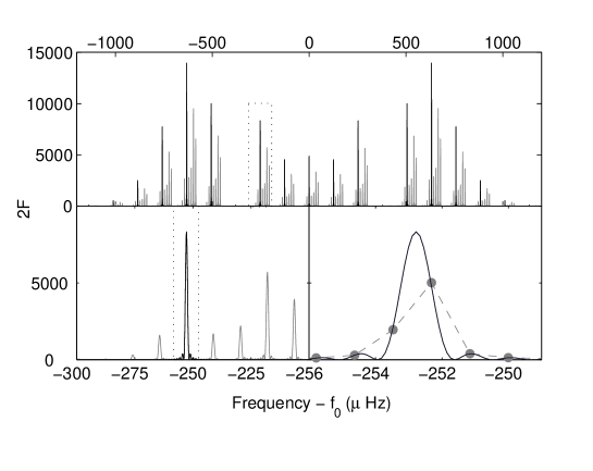
Figure 1: The $\mathcal{F}$-statistic as a function of frequency for a simulated signal with parameters $f_{0}=200+1.0849\times 10^{-6}$ Hz, $a=0.005$ sec, $P=7912.7$ sec, $\alpha=2.0$ rad, $\delta=1.0$ rad, and nuisance parameters $h_{0}=1$, $\psi=0.2$ rad, $\cos\iota=0.5$, $\Phi_{0}=1$ rad. The observation length is $T_{s}=T_{o}=10$ days with no gaps and a noiseless dataset (we have set $S_{h}=1$). In the upper panel we show $2\mathcal{F}$ (including AM sidebands) in solid grey, and $2\mathcal{F}$ neglecting the AM sidebands (as defined by equation 20) in solid black. The dotted box in the upper panel indicates the area magnified shown in the lower left panel where we can identify the amplitude modulation sidebands for this single frequency modulated sideband. The dotted box in the lower left panel indicates the magnified area shown in the lower right panel where we have included a third evaluation of $2\mathcal{F}$ through direct computation of equation 12 with frequency resolution $1/T_{s}$.

4 Searching for sources with unknown frequency - the sideband search

The search for continuously emitting sources is generally made more difficult when the intrinsic spin frequency of the source is unknown, and this is the case for LMXBs. We shall now describe a method for searching for these sources based on the incoherent summation of sideband $\mathcal{F}$-statistic. This technique is a fast way to search broad frequency bands for sources with known sky position and orbital period.

4.1 The sideband detection statistic

The majority of $\mathcal{F}$-statistic values from a source in a binary system are spread broadly across a relatively wide bandwidth ($\sim 4\pi f_{0}aT_{s}/P$ frequency bins) but are actually only present significantly in $\sim 4\pi f_{0}a$ isolated regions, each separated by $1/P$ Hz. We will define

$$q(f)=\sum_{n=-m}^{m}\delta(f-f^{\prime}_{n})$$ (21)

as an approximate search template where $f^{\prime}_{n}$ is the frequency of the closest frequency bin to the frequency of the $n$th sideband, equal to $f_{n}=f_{0}+n/P$. We have therefore constructed a comb of unit amplitude “spikes” each separated by $\approx 1/P$ Hz. We then convolve this template with the output of a wideband (sky position demodulated) $\mathcal{F}$-statistic search, $2\mathcal{F}(f)$ giving us

$$C(f)=2\mathcal{F}(f)\otimes q(f).$$ (22)

We should note that the number of “spikes” within the template is a function of the orbital radius and that an optimal value of $C(f)$ will be obtained if using its true value. However, the power of this detection statistic is sensitive only to large $\sim 50\%$ mismatches between template orbital radius and the true value and is therefore not required as an exactly known parameter. This procedure is many orders of magnitude faster than the equivalent coherent matched filtered search but, as we shall describe in the following section, this increase in speed comes at the cost of reduced sensitivity. An example of the sideband statistic $C(f)$ is shown in figure 3.

4.2 The sideband search sensitivity

The detection statistic $C(f)$ (equation 22) is simply the incoherent summation of sideband $\mathcal{F}$-statistics. In an idealised case of data free from gaps and with constant noise amplitude, our window function $W(f)$ can be expressed analytically and the detection statistic becomes

$$C(f)=\frac{1}{2}\sum_{n=-m}^{m}\left\{\frac{1-\cos\left[2\pi(\Delta f_{n})T\right]}{\left[\pi(\Delta f_{n})\right]^{2}}\right\}2\mathcal{F}(f_{n}).$$ (23)

We have used $\Delta f_{n}=f_{n}-f^{\prime}_{n}$ to represent the sideband frequency mismatches due to our finite frequency resolution. In practise $\Delta f_{0}$ will be drawn from a uniform distribution between the limits $[-\delta f/2-\delta f/2)$, and for the purposes of this analysis we shall assume that this is the case for $\Delta f_{n}$. For the noise only case, $2\mathcal{F}_{n}$ is a $\chi^{2}_{4}$-distributed random variable with mean and variance equal to $4$ and $8$ respectively. The simple summation of $M=2m+1$ such independent random variables results in a $\chi^{2}_{4M}$-distributed random variable. The mean and variance of $C$ for noise alone are then

$$\mu_{0}(C) = 4M,$$ (24)

$$\sigma^{2}_{0}(C) = 8M,$$ (25)

respectively. When a signal is present in the noise, $2\mathcal{F}_{n}$ becomes a non-centrally $\chi^{2}_{4}$-distributed with a non-centrality parameter $\lambda_{n}$ as a function of the random variable $\Delta f_{n}$. In order to approximate the distribution of $C$ in this case we use

$$2\mathcal{F}_{n}\left[\lambda_{n}(\Delta f_{n})\right]\approx|\tilde{W}(\Delta f_{n})|^{2}2\mathcal{F}_{n}(\lambda_{n}),$$ (26)

where we have assumed that for values of $|\tilde{W}(\Delta f_{n})|^{2}$ close to unity the change in the product of the $\mathcal{F}$ statistic with the window function is proportional to the relative change in the distribution mean. From this approximation it follows that the mean and variance for signal plus noise are

$$\mu_{1}(C) \approx \rho_{\mathrm{opt}}^{2}\langle|\tilde{W}|^{2}\rangle+4M,$$ (27)

$$\sigma^{2}_{1}(C) \approx \left(\frac{\rho_{\mathrm{opt}}^{4}}{M}+12\rho_{\mathrm{opt}}^{2}+24M\right)\left(\frac{\rho_{\mathrm{opt}}^{4}\langle|\tilde{W}|^{4}\rangle+8\rho_{\mathrm{opt}}^{2}\langle|\tilde{W}|^{2}\rangle+16M^{2}}{\rho_{\mathrm{opt}}^{4}+8\rho_{\mathrm{opt}}^{2}+16M^{2}}\right)$$ (28)

$$-8\rho_{\mathrm{opt}}^{2}\langle|\tilde{W}|^{2}\rangle-16M,$$

respectively, where

$$\sum_{n=-m}^{m}\lambda_{n}=\rho^{2}_{\mathrm{opt}}=\frac{2}{S_{h}(f_{0})}\int_{0}^{T_{s}}h^{2}(t)W(t)\rmd t.$$ (29)

and $\langle\ldots\rangle$ indicates an averaging over the range of possible values of $\Delta f_{n}$. By the central limit theorem we use the mean and variance approximations, in the case of signal plus noise, to describe the distributions of $C$ as Gaussian. Figure. 2 shows the relationship between search sensitivity, parameterised as $h_{0}\sqrt{T/S_{h}}$, as a function of $m$ and for various choices of frequency resolution $\delta f$.

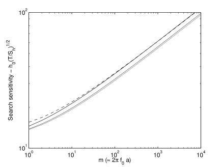
Figure 2: The sideband search sensitivity parameterised by $h_{0}\sqrt{T/S_{h}}$ for a $1\%$ false alarm rate and $10\%$ false dismissal rate averaged over the sky and as a function of $m$. We show in solid black, dark grey, and light grey, the curves corresponding to frequency resolutions of $1/T$, $1/2T$ and $1/4T$ respectively. The dashed black curve represents our approximation to the solid black curve using Gaussian distributions to model noise and signal plus noise distributions. Note that for large $m$ we see that the parameterised sensitivity is $\propto m^{1/4}$.

We can also use Equations 24, 25, 27 and 28 to provide a rough guide to the sensitivity by approximating the SNR achievable with this search as

$$\rho\sim\frac{\mu_{1}(C)-\mu_{0}(C)}{\sqrt{\sigma^{2}_{1}(C)}}\sim\rho_{\mathrm{opt}}^{2}\sqrt{\frac{M}{\rho_{\mathrm{opt}}^{4}+12M\rho_{\mathrm{opt}}^{2}+8M^{2}}}.$$ (30)

For $M\gg\rho_{\mathrm{opt}}^{2}$ we see for a given sideband search SNR that

$$h_{0}\propto M^{1/4}\sqrt{S_{h}/T}.$$ (31)

We should note that although this is an incoherent search technique, we still attain an $h_{0}$ sensitivity scaling proportional to $T^{-1/2}$, unlike most other incoherent searches. This is due to the fact that $M\approx 2(2\pi f_{0}a)+1$ is a constant for a given source and therefore the $M^{1/4}$ factor in equation 31 remains constant for any choice of observation time. The clear comparison here is to the stack-slide search [6] where the statistical behaviour of the detection statistic is very similar to the behaviour of the sideband statistic. For stack-slide however, the analogue of the parameter $M$ is the number of stacks, which have typically predefined length making the number of stacks proportional to the total observation time and consequently a $T^{-1/4}$ scaling is achieved.

5 A Follow up exploration of the $\mathcal{F}$-statistic likelihood

We propose using an MCMC approach with our $\mathcal{F}$-statistic signal model components (equations 15 and 16) to explore the associated likelihood space. This is a natural extension to the sideband search in which the $\mathcal{F}$-statistic and its components have already been computed from our GW dataset. By selecting values of the previous “sideband” search output, $C(f)$, above a predefined threshold, we identify isolated subspaces in our broadest parameter space dimension. These subspaces correspond to signal candidate frequencies and it is over this subset of frequencies that we perform the MCMC.

5.1 An MCMC exploration of the $\mathcal{F}$-statistic likelihood

In order to perform an MCMC we must calculate the likelihood. Let us first re-parameterise each $n$th complex $\mathcal{F}$-statistic components $F_{a}^{(n)}$ and $F_{b}^{(n)}$ as

$$F_{a}^{(n)}=\mathds{F}_{1}^{(n)}+i\mathds{F}_{3}^{(n)},\hskip 28.45274ptF_{b}^{(n)}=\mathds{F}_{2}^{(n)}+i\mathds{F}_{4}^{(n)},$$ (32)

where $n$ indexes the FM sidebands $(-m\leq n\leq m)$. For data containing signals in the presence of Gaussian noise the real variables $\mathds{F}^{(n)}_{i}$ are Gaussian distributed with means given by

$$\bar{\mathds{F}}_{1}^{(n)}=J_{n}(Z)T(AA_{1}+CA_{2})/4,\hskip 14.22636pt\bar{\mathds{F}}_{3}^{(n)}=-J_{n}(Z)T(AA_{3}+CA_{4})/4,$$

$$\bar{\mathds{F}}_{2}^{(n)}=J_{n}(Z)T(CA_{1}+BA_{2})/4,\hskip 14.22636pt\bar{\mathds{F}}_{4}^{(n)}=-J_{n}(Z)T(CA_{3}+BA_{4})/4,$$ (33)

and governed by a covariance matrix

$$\mathrm{cov}(\mathds{F}_{i}^{(n)},\mathds{F}_{j}^{(n)})=\left(\begin{array}[]{cc}\mathcal{C}&\mathcal{O}\\ \mathcal{O}&\mathcal{C}\\ \end{array}\right),\hskip 28.45274pt\mathcal{C}=\frac{TS_{h}}{8}\left(\begin{array}[]{cc}A&C\\ C&B\\ \end{array}\right),$$ (34)

where $\mathcal{O}$ indicates a null $2\times 2$ matrix. Therefore, the log likelihood function of the vector of $\mathcal{F}$-statistic components becomes

$$\mathcal{L}(\vec{\mathds{F}}) \propto -\sum_{n=-m}^{m}B\left[(\mathds{F}_{1}^{(n)}-\bar{\mathds{F}}_{1}^{(n)})^{2}+(\mathds{F}_{3}^{(n)}-\bar{\mathds{F}}_{3}^{(n)})^{2}\right]$$ (35)

$$+A\left[(\mathds{F}_{2}^{(n)}-\bar{\mathds{F}}_{2}^{(n)})^{2}+A(\mathds{F}_{4}^{(n)}-\bar{\mathds{F}}_{4}^{(n)})^{2}\right]$$

$$-2C\left[(\mathds{F}_{1}^{(n)}-\bar{\mathds{F}}_{1}^{(n)})(\mathds{F}_{2}^{(n)}-\bar{\mathds{F}}_{2}^{(n)})+(\mathds{F}_{3}^{(n)}-\bar{\mathds{F}}_{3}^{(n)})(\mathds{F}_{4}^{(n)}-\bar{\mathds{F}}_{4}^{(n)})\right].$$

We use an MCMC to efficiently explore this likelihood surface and to generate marginal posterior probability density functions (PDFs) for each of our search parameters. By using values of $C(f)$ above a given threshold we can think of this as an approximate identification of small volumes of parameter space $V_{i}$ likely to be associated with large values of the likelihood (or log-likelihood). By now treating $f_{0}$ as a search parameter within the MCMC we use $V_{i}$ as an approximation to our prior knowledge on that space by setting $p(f_{0}\notin V_{i})=0$. All subspaces $V_{i}$ are then considered to form a continuous space on frequency such that a positive frequency jump from within subspace $V_{i}$ large enough to fall just outside its upper boundary will land in subspace $V_{i+1}$. This way a single MCMC can be run and yield easily interpretable PDFs on our search space as opposed to separate PDFs for each frequency candidate which would leave us unable to make global parameter space inferences.

For our simple LMXB model we define the primary search parameters as $\Lambda=\left\{f_{0},h_{0},\cos\iota,\psi,\phi_{0},a,t_{p}\right\}$. The form of the signal as described in equations 15 and 16 shows us that the majority of $\mathcal{F}$-statistic is localised in $M$ sidebands at frequencies $f_{0}+n/P$. In the simplest cases this allows us to compute the log likelihood using only $4M$ data points (ie. each of the $4$ $\mathcal{F}$-statistic components sampled at the closest discrete frequency bin $f^{\prime}_{n}$ to each sideband). Data used between sidebands would add only an identical constant factor to each computation of the log-likelihood for all $\Lambda$ thus giving no useful discriminating information. By not using inter-sideband data the burden of the computation of $\mathcal{L}$ is therefore reduced by a factor of $\sim T/P$ and is therefore independent of observation time. We should also note that for our simplistic phase model each computation of $\mathcal{L}$ requires only a recalculation of the $\mathcal{F}$-statistic component means (equation 33) for each of the $M$ sidebands. Figure. 3 shows a set of marginal posterior distributions for an example LMXB type problem. We should also note that this MCMC stage alone is suited to the search for GWs from AMXPs for which the frequency and orbital parameters are known apriori to relatively high accuracy.

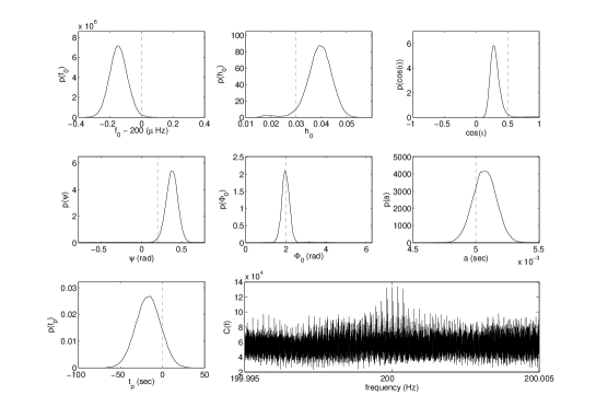
Figure 3: The marginal posterior PDFs (solid black lines) for an example LMXB type problem and the corresponding sideband detection statistic (lower right). The broken grey lines in the PDF plots indicate the true parameter values. The detector noise is assumed known at $S_{h}=1$ and the observation time is $10$ days which for the chosen signal parameters results in an optimal SNR of $?$. The search band is $0.01$ Hz from which the $20$ largest values of $C$ were used as candidates for the MCMC prior frequency ranges.

6 Summary

We have presented a new incoherent search technique designed for performing GW searches for known objects in binary systems with unknown or poorly known frequencies, specifically LMXBs. Accurate knowledge of the orbital period allows the incoherent summation of frequency modulated $\mathcal{F}$-statistic sidebands removing orbital phase as a search parameter and also relaxing the requirement for accurate knowledge of orbital radius. Of course, all of these benefits come at the price of reduced sensitivity to GW amplitude which we have shown to scale as $h_{0}\propto(4\pi f_{0}a)^{1/4}T^{1/2}$ implying that greatest sensitivity is achieved for short period (small orbital radius) binaries. Full implementation of the search pipeline will take advantage of the multi-interferometer $\mathcal{F}$-statistic [28] whereby prior to the summation of sideband power data sets from $N$ independent detectors are combined coherently thereby increasing sensitivity by $\sim\sqrt{N}$ for little additional computational cost. We have also identified that the coherent follow up MCMC stage constitutes a complete search if applied to the AMXPs, a similar class of source to the LMXBs but for which the frequency and orbital parameters are well constrained apriori. We again stress that here we have applied the proposed pipeline only to a simple source model and neglected issues such as poorly known orbital period and sky position, non-zero eccentricity, realistic detector noise characteristics and more complex issues such as the detailed spin frequency evolution of accreting systems. However, we believe that solutions to these problems can be integrated into this search pipeline and are described in detail in [15, 16]. Finally, we stress that although the final search stage is a coherent one, the ultimate sensitivity of the complete pipeline is limited by the threshold set in the incoherent “sideband” search stage.

References

- [1] The LIGO Scientific Collaboration 2004 Phys. Rev. D 69 082004–+
- [2] The LIGO Scientific Collaboration 2005 Phys. Rev. Lett 94 181103–+
- [3] The LIGO Scientific Collaboration 2005 Phys. Rev. D 72 102004–+
- [4] The LIGO Scientific Collaboration 2006 Coherent searches for periodic gravitational waves from unknown isolated sources and scorpius x-1: results from the second ligo science run Preprint gr-qc/0605028
- [5] Ballmer S W 2006 Class. Quantum Grav. 23 179
- [6] Brady P R, Creighton T, Cutler C and Schutz B F 1998 Phys. Rev. D 57 2101–2116
- [7] Ransom S M, Cordes J M and Eikenberry S S 2003 Astrophys. J. 589 911–920
- [8] Wijnands R and van der Klis M 1998 Nat. 394 344–346
- [9] Markwardt C B, Swank J H, Strohmayer T E Zand J J M i and Marshall F E 2002 Astrophys. J. Lett 575 L21–L24
- [10] Galloway D K, Chakrabarty D, Morgan E H and Remillard R A 2002 Astrophys. J. Lett 576 L137–L140
- [11] Markwardt C B, Smith E and Swank J H 2003 IAU circ. 8080 2–+
- [12] Markwardt C B and Swank J H 2003 IAU circ. 8144 1–+
- [13] Galloway D K, Markwardt E H, Morgan E H, Chakrabarty D and Strohmayer T E 2005 Astrophys. J. Lett 622 L45–L48
- [14] Kaaret P, Morgan E H, Vanderspek R and Tomsick J A 2006 Astrophys. J. 638 963–967
- [15] Messenger C and Woan G in preparation
- [16] Messenger C and Woan G in preparation
- [17] White N E and Xhang W 1997 Astrophys. J. Lett 490 L87+
- [18] Bildsten L 1998 Astrophys. J. Lett 501 L89+
- [19] Andersson N 1998 Astrophys. J. 502 708–+
- [20] Ushomirsky G, Cutler C and Bildsten L 2000 Mon. Not. R. Astron. Soc. 319 902–932
- [21] Andersson N, Glampedakis K, Haskell B and Watts A L 2005 Mon. Not. R. Astron. Soc. 361 1153–1164
- [22] Ritter H and Kolb U 2003, Astron. & Astrophys. 404, 301
- [23] Bildsten L 2000 American Institute of Physics Conference Series 522 359–369
- [24] van der Klis M 2000 Annual Review of Astronomy and Astrophysics 38 717–760
- [25] Wijnands R, van der Klis M, Homan J, Chakrabarty D, Markwardt C B and Morgan E H 2003 Nat. 424 44–47
- [26] Linares M, van der Klis M, Altamirano D and Markwardt C B 2005 Astrophys. J. 634 1250–1260
- [27] Jaranowski P, Królak A and Schutz B F 1998 Phys. Rev. D 58 063001–+
- [28] Cutler C and Schutz B F 2005 Phys. Rev. D 72 063006–+