Constraint Damping in First-Order Evolution Systems for Numerical Relativity

Abstract

A new constraint suppressing formulation of the Einstein evolution equations is presented, generalizing the five-parameter first-order system due to Kidder, Scheel and Teukolsky (KST). The auxiliary fields, introduced to make the KST system first-order, are given modified evolution equations designed to drive constraint violations toward zero. The algebraic structure of the new system is investigated, showing that the modifications preserve the hyperbolicity of the fundamental and constraint evolution equations. The evolution of the constraints for pertubations of flat spacetime is completely analyzed, and all finite-wavelength constraint modes are shown to decay exponentially when certain adjustable parameters satisfy appropriate inequalities. Numerical simulations of a single Schwarzschild black hole are presented, demonstrating the effectiveness of the new constraint-damping modifications.

I Introduction

Numerical relativity has recently undergone a revolution. Multiple research groups, using a variety of mathematical and computational formalisms, have produced consistent pictures of the late inspiral and coalescence of binary black hole systems Pretorius (2005a); Campanelli et al. (2006a, b, c); Baker et al. (2006a, b); Scheel et al. (2006); Brügmann et al. (2006), a goal that until recently seemed remote. The community is opening a theoretical window on issues fundamental to gravitational wave astrophysics, but much work still remains to be done.

State of the art simulations have provided gravitational waveforms due to the last several orbits of a binary black hole system, and its eventual coalescence and ringdown. This is an extraordinary achievement, but numerical relativity may need to handle well over a dozen orbits accurately before a seamless transition can be made from post-Newtonian analysis. This requires an exceptionally stable evolution scheme, and also an extremely efficient one, if the simulations are to be done in a timely manner.

Numerical simulations can become unstable for a variety of reasons, some purely numerical (such as a poor choice of algorithm), some purely mathematical (such as ill-posedness of the continuum mathematical problem), and some a combination of the two. The subject of this paper is an instability of this last type: the exponential growth of the constraint fields under free evolution – an instability of the continuum evolution equations, seeded by numerical errors.

A variety of methods exist to deal with such instabilities. One very well established method is known as constrained evolution Stark and Piran (1985); Abrahams and Evans (1992); Choptuik (1993); Abrahams and Evans (1993); Abrahams et al. (1994); Choptuik et al. (2003a, b); Rinne (2005), in which some subset of the dynamical fields are integrated in time using the evolution equations, and others are obtained by solving the constraints after each time step. This separation of the fields into an “evolved” family and a “constrained” family is normally guided by some sort of symmetry. A related method, known as constraint projection Anderson and Matzner (2005); Holst et al. (2004), places all fields on an equal footing, freely integrating everything using the evolution equations, then periodically “projecting” the fields down to the constraint-satisfying subset of the solution space. It appears that this method can be quite robust in practice, but it can also be technically demanding, requiring the repeated solution of nonlinear elliptic equations.

A preferable approach for dealing with these instabilities, whenever possible, is to remove them from the evolution system at the continuum level, before they reach the numerical code. This type of effort is often referred to as “constraint damping.” It is possible to change the evolution equations without changing the physics they represent. For instance, coordinates can be chosen freely on the simulated spacetime, and indeed, careful choices of gauge have been shown to have a strong effect on the stability of simulations, particularly in the BSSN system Alcubierre et al. (2003); Yo et al. (2002); Gundlach and Martin-Garcia (2006); van Meter et al. (2006). Another, perhaps more drastic method to stabilize constraints involves extending the family of evolved fields. It is possible, with some care, to introduce fields whose evolution will naturally lead to the presence of friction terms in the implied constraint evolution system. Systems of this form have come to be referred to as “$\lambda$ systems” in the relativity literature, after the pioneering work of Brodbeck et al. Brodbeck et al. (1999); Siebel and Hübner (2001).

The constraint damping of Ref. Brodbeck et al. (1999) utilizes the freedom to substitute constraint equations into the evolution equations. In the physical situation where the constraints are all satisfied, the equations are unchanged. However in the numerical situation where the constraint satisfaction is at best approximate, these substitutions can have a profound effect on the structure of the evolution system and the stability of its constraints. In Ref. Kidder et al. (2001), Kidder, Scheel and Teukolsky added terms, proportional to the constraints, to a first-order representation of the Arnowitt-Deser-Misner (ADM) evolution equations Arnowitt et al. (1962) (starting from the form advocated by York York (1979)). With these modifications, they were able to change the principal part of the evolution system. When the free parameters satisfy certain inequalities, the evolution system becomes strongly, or symmetric, hyperbolic Kidder et al. (2001); Lindblom and Scheel (2002, 2003); Kidder et al. (2005). The purpose of the present paper is to generalize the KST systems even further, to add more terms proportional to constraints into the evolution equations, but now with the goal of damping the constraints while preserving hyperbolicity. It will be shown that this goal can largely be achieved, stabilizing all the constraints of the KST systems, without the need to introduce extra fields as in the “$\lambda$ system” approach.

The possibility of constraint damping along these lines is now widely seen as a major advantage of the generalized harmonic formalism. Pretorius Pretorius (2005b, a), building on Gundlach et al. Gundlach et al. (2005), introduced such a modification in his generalized harmonic evolution code, leading to the first ever simulation of a full orbit and merger of binary black holes. In Ref. Lindblom et al. (2006), this system was converted into an explicitly first-order, linearly degenerate, symmetric-hyperbolic form. An extensive body of mathematical literature exists on systems of this form, and they are also very well suited to highly accurate multidomain pseudospectral collocation methods. While this first-order generalized harmonic system is perfectly acceptable for numerical relativity, and indeed is now used for nearly all simulations currently being done by the Caltech and Cornell numerical relativity groups, there would be considerable value in implementing a KST system of comparable stability. For one thing, the KST system involves just over half as many fields as the first-order generalized harmonic system, so it could provide a considerable improvement in code runtime. The KST systems are also closer to the evolution systems used historically in numerical relativity. Gauge is specified again in terms of (densitized) lapse and shift. So a large body of research on gauge conditions can be more easily applied.

As the standard KST systems already have adjustable parameters, it is an interesting question whether any of them can have constraint-damping properties. Even without calculations, it is clear that the answer must be “no.” With the generalized-harmonic system presented in Ref. Lindblom et al. (2006), two parameters are available, $\gamma_{0}$ and $\gamma_{2}$, which tune the stability of small constraint-violating perturbations of flat spacetime. The inverses of these parameters (up to factors of order unity) define timescales on which short-wavelength constraint modes will decay exponentially. All of the free parameters of the standard KST systems are dimensionless, so they cannot fix any preferred timescale for the damping of perturbations of flat spacetime. Of course in the full nonlinear phase space, the dimensions necessary for such a timescale can be provided by nontrivial features of a particular solution, for instance the mass of a black hole. Indeed, in Ref. Scheel et al. (2002), it was demonstrated that careful fine-tuning of the parameters can considerably extend the lifetime of a black hole simulation. This effect cannot really be considered constraint damping, though, as the optimum choice of parameters depends strongly on the details of the initial data, and in fact it must fail for small features in asymptotic regions, where the above flat space arguments begin to apply.

In the present paper, the KST systems will be generalized even further, introducing one new free parameter with dimensions of inverse-time, that can be considered a mechanism for constraint damping. This generalization is directly analogous to methods used in the past Holst et al. (2004); Lindblom et al. (2006) for controlling the stability of the constraints that appear when an evolution system that is second-order in spatial derivatives is reduced to first-order form by the introduction of auxiliary fields. Such a constraint exists in the KST systems, and while our methods are only designed to control this particular constraint, the intricate coupling of the constraints, in their evolution, extends the constraint damping effect to all (finite wavelength) constraint modes, including the Hamiltonian and momentum constraints.

The format of this paper is as follows. In Sec. II the intuitive mechanism behind the new constraint damping terms is sketched out in the context of a simple toy model. In Sec. III, analogous modifications are applied to the five-parameter KST evolution systems, and conditions on these modifications are noted to keep the resulting system hyperbolic. In Sec. IV, the hyperbolicity of the constraint evolution system is investigated. In Sec. V the effectiveness of these modifications on constraint-violating perturbations of flat spacetime is seen in detail. In Sec. VI, the available parameter freedom is summarized, and in Sec. VII, results are presented of a few simple numerical simulations using this new evolution system.

II Illustration of a Simple Model System

Before jumping into the full equations of general relativity, it would be instructive to outline the constraint damping idea in the context of the simplest hyperbolic system, the scalar wave equation:

$$\eta^{\mu\nu}\partial_{\mu}\partial_{\nu}\psi=0,$$ (1)

for a real scalar field $\psi$, where $\eta_{\mu\nu}$ is the Minkowski metric in Cartesian coordinates. This equation involves only one field, and no constraints, but it is second-order in both space and time. The second-order derivatives are removed by promoting the first derivatives of $\psi$ to independent fields. The first time derivative (up to a conventional minus sign) will be denoted with the symbol $\pi$. The wave equation now becomes the system:

$$\partial_{t}\psi = -\pi,$$ (2)

$$\partial_{t}\pi = -\delta^{ij}\partial_{i}\partial_{j}\psi,$$ (3)

where latin indices refer to the spatial coordinates of the chosen inertial frame. The one-form $\phi_{i}$, defined by a new constraint ${\cal C}_{i}$, can be used to remove second spatial derivatives from the system:

$$\partial_{t}\psi = -\pi,$$ (4)

$$\partial_{t}\pi = -\delta^{ij}\partial_{i}\phi_{j},$$ (5)

$${\cal C}_{i} := \partial_{i}\psi-\phi_{i}=0.$$ (6)

Before this can be useful for free evolution, an equation is needed for evolving $\phi_{i}$. This equation is commonly derived by equating the spatial coordinate derivatives of both sides of Eq. (4), commuting partial derivatives on the left, and substituting the constraint to find:

$$\partial_{t}\phi_{i}=-\partial_{i}\pi.$$ (7)

This equation closes the evolution system, and leaves us with a nice first-order symmetric-hyperbolic representation of the scalar wave equation. However the newly defined constraint field is only marginally stable. As is easily verified by direct substitution of the constraint definition and the evolution equations, the constraint is now conserved:

$$\partial_{t}{\cal C}_{i}=0.$$ (8)

This shows that exact constraint satisfaction should be preserved within the domain of dependence of the initial data, but also that any violations that may arise will be preserved as well.

Because the constraint is linear in undifferentiated $\phi_{i}$, anything added to the right side of Eq. (7) will transfer directly to the evolution equation implied for the constraint. For example, if the equation is changed to:

$$\partial_{t}\phi_{i} = -\partial_{i}\pi+\gamma{\cal C}_{i}$$ (9)

$$= -\partial_{i}\pi+\gamma(\partial_{i}\psi-\phi_{i}),$$ (10)

for some constant $\gamma$, then the constraint-satisfying solution space is unchanged, but the evolution of the constraint becomes

$$\partial_{t}{\cal C}_{i}=-\gamma{\cal C}_{i}.$$ (11)

Thus, with this method, the constraint can be damped (assuming hyperbolicity is preserved) exponentially on an arbitrary fixed timescale $\gamma^{-1}$. As we will see when we discuss the KST system, the constraint damping effect can extend even farther than the constraint that appears in the reduction. Even those constraints that exist before the reduction to first-order form can be damped.

The question of whether this modification preserves the clear symmetric hyperbolicity of the standard reduction is important, and a very simple argument shows that hyperbolicity is not affected. If a linear change of variables is made (in other words, a change of basis on the vector bundle of dynamical fields), defining $\bar{\pi}:=\pi-\gamma\psi$, then all modifications of the principal part of the fundamental evolution system disappear:

$$\partial_{t}\psi \simeq 0,$$ (12)

$$\partial_{t}\bar{\pi} \simeq -\delta^{ij}\partial_{i}\phi_{j},$$ (13)

$$\partial_{t}\phi_{i} \simeq -\partial_{i}\bar{\pi}$$ (14)

(the symbol “$\simeq$” means that all nonprincipal – in this case, algebraic – terms have been omitted). This transformed system is exactly the same as the unmodified system at principal order, and is clearly symmetric-hyperbolic. The existence of a positive-definite symmetrizing inner product is independent of the basis of dynamical fields. Indeed, the obvious symmetrizer for the transformed system,

$$dS^{2} = \Lambda d\psi^{2}+d{\bar{\pi}}^{2}+\delta^{ij}d\phi_{i}d\phi_{j},$$ (15)

$$= \Lambda d\psi^{2}+(d\pi-\gamma d\psi)^{2}+\delta^{ij}d\phi_{i}d\phi_{j},$$ (16)

when expressed in terms of $\pi$, is positive-definite (for positive $\Lambda$) and symmetrizes the untransformed system. Therefore, this constraint-damped form of the scalar wave system is symmetric-hyperbolic for any fixed choice of the damping timescale.

III The Modified KST Evolution System

The Kidder-Scheel-Teukolsky Kidder et al. (2001) evolution equations are a five-parameter generalization of the standard first-order representation of the classic ADM Arnowitt et al. (1962) equations, in the form advocated by York York (1979):

$$\partial_{t}g_{ij}-{\cal L}_{\vec{N}}g_{ij} = -2NK_{ij}$$ (17)

$$\partial_{t}K_{ij}-{\cal L}_{\vec{N}}K_{ij} = NR_{ij}+N(KK_{ij}-2{K_{i}}^{k}K_{kj})$$ (18)

$$-\nabla_{i}\nabla_{j}N.$$

The dynamical fields are $\{g_{ij},K_{ij}\}$, the metric intrinsic to the slice of constant $t$, and the extrinsic curvature of its embedding in spacetime. The gauge fields $\{N,N^{i}\}$, lapse and shift, determine the evolution of the coordinates.

The Ricci tensor $R_{ij}$ written above is that of the spatial metric $g_{ij}$, so it implicitly involves second spatial derivatives of $g_{ij}$. The evolution system can be reduced to first-order form by promoting the partial derivatives of the spatial metric functions to an independent (nontensorial) three-index field:

$$D_{kij}:=\frac{1}{2}\partial_{k}g_{ij}.$$ (19)

As long as $D_{kij}$, under its own evolution, properly represents $\partial_{k}g_{ij}/2$, it can be substituted for any derivatives of $g_{ij}$. This renders the ADM system first-order.

This evolution system, like that for the scalar field, describes physics only when certain constraint fields vanish:

$${\cal C} := \frac{1}{2}(R-K_{ij}K^{ij}+K^{2}),$$ (20)

$${\cal C}_{i} := \nabla^{j}(K_{ij}-Kg_{ij}),$$ (21)

$${\cal C}_{kij} := \partial_{k}g_{ij}-2D_{kij}.$$ (22)

The Hamiltonian and momentum constraints, ${\cal C}$ and ${\cal C}_{i}$, must vanish (in vacuum) throughout each spatial slice, according to the four Einstein equations not represented in Eq. (18). The three-index constraint ${\cal C}_{kij}$ vanishes when $D_{kij}$ properly represents $\partial_{k}g_{ij}/2$, in analogy with the constraint of the scalar field system.

The new field, $D_{kij}$, is to be considered independent in free evolution. An evolution equation must be defined for this field, one that is consistent with the satisfaction of the three-index constraint above. The equation analogous to Eq. (7) is

$$\hat{\partial}_{0}D_{kij} = \frac{1}{2}\partial_{k}(\hat{\partial}_{0}g_{ij}),$$ (23)

$$= -\partial_{k}(NK_{ij}),$$ (24)

where the shorthand $\hat{\partial}_{0}$ refers to the derivative, $\partial_{t}-{\cal L}_{\vec{N}}$, along the normal to the spatial slice.

The evolution system has now been written in first-order form, and we can begin to ask about its hyperbolicity. Kidder, Scheel and Teukolsky Kidder et al. (2001) have shown that the above system can be rendered strongly hyperbolic with a few simple modifications. The first of these is commonly referred to as densitization of the lapse. Rather than fixing $N$ directly, we fix a related field $Q$ defined by

$$N=g^{\gamma_{0}}\exp(Q),$$ (25)

where $g$ is the determinant of $g_{ij}$ and $\gamma_{0}$ is a constant nonzero parameter. The occurences of $\partial_{k}g_{ij}$ that then arise arise from the $\nabla_{i}\nabla_{j}N$ term in Eq. (18) are then replaced by $2D_{kij}$. The second modification required for hyperbolicity is the addition of terms to the evolution equations for $K_{ij}$ and $D_{kij}$, that are proportional to the constraints:

$$\hat{\partial}_{0}K_{ij} = ...+\gamma_{1}Ng_{ij}{\cal C}+\gamma_{2}Ng^{ab}{\cal C}_{a(ij)b},$$ (26)

$$\hat{\partial}_{0}D_{kij} = ...+\frac{1}{2}\gamma_{3}Ng_{k(i}{\cal C}_{j)}+\frac{1}{2}\gamma_{4}Ng_{ij}{\cal C}_{k},$$ (27)

where the ellipses refer to the right sides of Eqs. (18) and (24). The four-index object ${\cal C}_{klij}:=2\partial_{[k}D_{l]ij}$ used here can be thought of as another constraint, but it vanishes automatically whenever the three-index constraint vanishes. The parameters $\{\gamma_{0},...,\gamma_{4}\}$ do not affect the physical solution space of the equations in any way, but they directly affect the principal part of the evolution system. In Ref. Kidder et al. (2001), Kidder, Scheel and Teukolsky determined sufficient conditions for these parameters that render the evolution system strongly hyperbolic. In Ref. Lindblom and Scheel (2003) and an appendix of Ref. Kidder et al. (2005), these arguments were extended, and it was also made clear on what subset of the parameter space the equations satisfied the stronger condition of symmetric hyperbolicity.

The focus of this paper is a further modification of Eq. (27) along the same lines as that described in Sec. II. Here the goal is to modify the evolution of the three-index constraint, which in the ordinary KST system is implied to evolve as

$$\hat{\partial}_{0}{\cal C}_{kij}=-\gamma_{3}Ng_{k(i}{\cal C}_{j)}-\gamma_{4}Ng_{ij}{\cal C}_{k}.$$ (28)

Note that the need for damping here is more dire than in the scalar field case. Hyperbolicity requires $\gamma_{3}$ and $\gamma_{4}$ to be nonzero, so any violation of the momentum constraint will feed directly into the three-index constraint. This is countered as in the previous section by including terms proportional to the three-index constraint in the evolution equation for $D_{kij}$. As we will see in a moment, multiples of the traces, denoted ${\cal C}^{1}_{k}:=g^{ij}{\cal C}_{kij}$ and ${\cal C}^{2}_{j}:=g^{ki}{\cal C}_{kij}$, must be added in separately, so the resulting evolution equation is:

$$\hat{\partial}_{0}D_{kij} = ...+\frac{1}{2}\gamma_{3}Ng_{k(i}{\cal C}_{j)}+\frac{1}{2}\gamma_{4}Ng_{ij}{\cal C}_{k}$$ (29)

$$+\frac{1}{2}N\gamma_{5}{\cal C}_{kij}+\frac{1}{2}N\gamma_{6}{\cal C}^{1}_{k}g_{ij}$$

$$+\frac{1}{2}N\gamma_{7}{\cal C}^{2}_{(i}g_{j)k}+\frac{1}{2}N\gamma_{8}{\cal C}^{1}_{(i}g_{j)k}$$

$$+\frac{1}{2}N\gamma_{9}{\cal C}^{2}_{k}g_{ij}.$$

The term proportional to $\gamma_{5}$ is analogous to the term proportional to $\gamma$ in Eq. (9). The terms proportional to $\gamma_{6}$, $\gamma_{7}$, $\gamma_{8}$ and $\gamma_{9}$ are necessitated by the hyperbolicity conditions, which we now consider.

The principal part of this system is:

$${\hat{\partial}}_{0}g_{ij} \simeq 0,$$ (30)

$${\hat{\partial}}_{0}K_{ij} \simeq N[g^{ab}\delta^{c}_{i}\delta^{d}_{j}-(1+\gamma_{2})g^{ad}\delta^{b}_{(i}\delta^{c}_{j)}$$ (31)

$$-(1-\gamma_{2})g^{bc}\delta^{a}_{(i}\delta^{d}_{j)}+(1+2{\gamma_{0}})g^{cd}\delta^{a}_{(i}\delta^{b}_{j)}$$

$$-\gamma_{1}g^{ad}g^{bc}g_{ij}+\gamma_{1}g^{ab}g^{cd}g_{ij}]\partial_{a}D_{bcd},$$

$${\hat{\partial}}_{0}D_{kij} \simeq -N[\delta^{c}_{k}\delta^{a}_{i}\delta^{b}_{j}-\frac{1}{2}\gamma_{3}g^{ca}g_{k(i}\delta^{b}_{j)}$$ (32)

$$-\frac{1}{2}\gamma_{4}g^{ca}g_{ij}\delta^{b}_{k}+\frac{1}{2}\gamma_{3}g^{ab}g_{k(i}\delta^{c}_{j)}$$

$$+\frac{1}{2}\gamma_{4}g^{ab}g_{ij}\delta^{c}_{k}]\partial_{c}K_{ab}$$

$$+N[\frac{1}{2}\gamma_{5}\delta^{c}_{k}\delta^{a}_{i}\delta^{b}_{j}+\frac{1}{2}\gamma_{6}\delta^{c}_{k}g^{ab}g_{ij}$$

$$+\frac{1}{2}\gamma_{7}g^{ca}\delta^{b}_{(i}g_{j)k}+\frac{1}{2}\gamma_{8}g^{ab}\delta^{c}_{(i}g_{j)k}$$

$$+\frac{1}{2}\gamma_{9}g^{ca}\delta^{b}_{k}g_{ij}]\partial_{c}g_{ab}.$$

Hyperbolicity is well established for the standard KST system, $\gamma_{5}=\gamma_{6}=...=\gamma_{9}=0$, so as in Sec. II, it is best to seek a linear change of variables to reduce the constraint-damped system to the standard system. Continuing the analogy with the scalar field, define

$$\bar{K}_{ij}:=K_{ij}-\frac{1}{2}\gamma_{5}g_{ij}.$$ (33)

Then the equation for $\hat{\partial}_{0}\bar{K}_{ij}$ has the same principal part as that for $\hat{\partial}_{0}K_{ij}$. The equation for $\hat{\partial}_{0}D_{kij}$ becomes

$${\hat{\partial}}_{0}D_{kij} \simeq -N[\delta^{c}_{k}\delta^{a}_{i}\delta^{b}_{j}-\frac{1}{2}\gamma_{3}g^{ca}g_{k(i}\delta^{b}_{j)}$$ (34)

$$-\frac{1}{2}\gamma_{4}g^{ca}g_{ij}\delta^{b}_{k}+\frac{1}{2}\gamma_{3}g^{ab}g_{k(i}\delta^{c}_{j)}$$

$$+\frac{1}{2}\gamma_{4}g^{ab}g_{ij}\delta^{c}_{k}]\partial_{c}\bar{K}_{ab}$$

$$+N[\frac{1}{2}(\gamma_{6}-\frac{1}{2}\gamma_{4}\gamma_{5})\delta^{c}_{k}g^{ab}g_{ij}$$

$$+\frac{1}{2}(\gamma_{7}+\frac{1}{2}\gamma_{3}\gamma_{5})g^{ca}\delta^{b}_{(i}g_{j)k}$$

$$+\frac{1}{2}(\gamma_{8}-\frac{1}{2}\gamma_{3}\gamma_{5})g^{ab}\delta^{c}_{(i}g_{j)k}$$

$$+\frac{1}{2}(\gamma_{9}+\frac{1}{2}\gamma_{4}\gamma_{5})g^{ca}\delta^{b}_{k}g_{ij}]\partial_{c}g_{ab}.$$

If, for arbitrary $\gamma_{5}$, the further parameters are fixed as

$$\gamma_{6} = \frac{1}{2}\gamma_{4}\gamma_{5}$$ (35)

$$\gamma_{7} = -\frac{1}{2}\gamma_{3}\gamma_{5}$$ (36)

$$\gamma_{8} = \frac{1}{2}\gamma_{3}\gamma_{5}$$ (37)

$$\gamma_{9} = -\frac{1}{2}\gamma_{4}\gamma_{5},$$ (38)

then the principal system, in the transformed variables, loses any reference to $\gamma_{5},...,\gamma_{9}$.

$${\hat{\partial}}_{0}g_{ij} \simeq 0,$$ (39)

$${\hat{\partial}}_{0}\bar{K}_{ij} \simeq N[g^{ab}\delta^{c}_{i}\delta^{d}_{j}-(1+\gamma_{2})g^{ad}\delta^{b}_{(i}\delta^{c}_{j)}$$ (40)

$$-(1-\gamma_{2})g^{bc}\delta^{a}_{(i}\delta^{d}_{j)}+(1+2{\gamma_{0}})g^{cd}\delta^{a}_{(i}\delta^{b}_{j)}$$

$$-\gamma_{1}g^{ad}g^{bc}g_{ij}+\gamma_{1}g^{ab}g^{cd}g_{ij}]\partial_{a}D_{bcd},$$

$${\hat{\partial}}_{0}D_{kij} \simeq -N[\delta^{c}_{k}\delta^{a}_{i}\delta^{b}_{j}-\frac{1}{2}\gamma_{3}g^{ca}g_{k(i}\delta^{b}_{j)}$$ (41)

$$-\frac{1}{2}\gamma_{4}g^{ca}g_{ij}\delta^{b}_{k}+\frac{1}{2}\gamma_{3}g^{ab}g_{k(i}\delta^{c}_{j)}$$

$$+\frac{1}{2}\gamma_{4}g^{ab}g_{ij}\delta^{c}_{k}]\partial_{c}\bar{K}_{ab}.$$

This is the principal part of the standard KST system. So for any value of the parameter $\gamma_{5}$, with $\gamma_{6},...,\gamma_{9}$ fixed by Eqs. (35) – (38), the hyperbolicity of our modified system is the same as that of the corresponding standard KST system.

IV Hyperbolicity of the constraint evolution

Let us now turn our attention to the evolution of the constraint fields in our modified KST evolution system. Given the definitions of the constraints in terms of the fundamental dynamical fields, an evolution system for the constraints follows from our fundamental evolution equations. It is important, for the construction of constraint-preserving boundary conditions, that this system also be symmetric-hyperbolic  Kidder et al. (2005); Stewart (1998); Calabrese et al. (2003). The principal part of this evolution system can be expressed as,

$$\hat{\partial}_{0}{\cal C} \simeq -\frac{1}{2}(2-\gamma_{3}+2\gamma_{4})Ng^{ij}\partial_{i}{\cal C}_{j}$$ (42)

$$+\frac{1}{2}(\gamma_{8}-2\gamma_{6}-\gamma_{5})Ng^{ij}\partial_{i}{\cal C}^{1}_{j}$$

$$+\frac{1}{2}(\gamma_{7}-2\gamma_{9}+\gamma_{5})Ng^{ij}\partial_{i}{\cal C}^{2}_{j},$$

$$\hat{\partial}_{0}{\cal C}_{i} \simeq -(1+2\gamma_{1})N\partial_{i}{\cal C}$$ (43)

$$+\frac{1}{2}Ng^{kl}g^{ab}\bigl{[}(1-\gamma_{2})\partial_{k}{\cal C}_{labi}+(1+\gamma_{2})\partial_{k}{\cal C}_{ailb}$$

$$\quad\qquad\qquad-(1+2{\gamma_{0}})\partial_{k}{\cal C}_{liab}\bigr{]},$$

$$\hat{\partial}_{0}{\cal C}_{kij} \simeq 0,$$ (44)

$$\hat{\partial}_{0}{\cal C}_{abij} \simeq -\frac{1}{2}N\gamma_{3}g_{i[a}\partial_{b]}{\cal C}_{j}-\frac{1}{2}N\gamma_{3}g_{j[a}\partial_{b]}{\cal C}_{i}$$ (45)

$$-N\gamma_{4}g_{ij}\partial_{[b}{\cal C}_{a]}-N\gamma_{6}g_{ij}\partial_{[b}{\cal C}^{1}_{a]}$$

$$-\frac{1}{2}N\gamma_{7}g_{i[a}\partial_{b]}{\cal C}^{2}_{j}-\frac{1}{2}N\gamma_{7}g_{j[a}\partial_{b]}{\cal C}^{2}_{i}$$

$$-\frac{1}{2}N\gamma_{8}g_{i[a}\partial_{b]}{\cal C}^{1}_{j}-\frac{1}{2}N\gamma_{8}g_{j[a}\partial_{b]}{\cal C}^{1}_{i}$$

$$-N\gamma_{9}g_{ij}\partial_{[b}{\cal C}^{2}_{a]},$$

where the four-index object ${\cal C}_{klij}:=2\partial_{[k}D_{l]ij}$ is considered an independent constraint, so that the constraint evolution system is first-order.

The inclusion of the terms proportional to $\gamma_{5},...,\gamma_{9}$ in Eqs. (42) – (45) has seriously complicated this system. Let us consider, however, the case considered above, where $\gamma_{5}$ is arbitrary, and the other parameters are fixed by Eqs. (35) – (38). In this case, a number of remarkable simplifications occur and the above system can be written as

$$\hat{\partial}_{0}{\cal C} \simeq -\frac{1}{2}(2-\gamma_{3}+2\gamma_{4})Ng^{ij}\partial_{i}\bar{\cal C}_{j},$$ (46)

$$\hat{\partial}_{0}\bar{\cal C}_{i} \simeq -(1+2\gamma_{1})N\partial_{i}{\cal C}$$ (47)

$$+\frac{1}{2}Ng^{kl}g^{ab}\bigl{[}(1-\gamma_{2})\partial_{k}{\cal C}_{labi}+(1+\gamma_{2})\partial_{k}{\cal C}_{ailb}$$

$$\quad\qquad\qquad-(1+2{\gamma_{0}})\partial_{k}{\cal C}_{liab}\bigr{]},$$

$$\hat{\partial}_{0}{\cal C}_{kij} \simeq 0,$$ (48)

$$\hat{\partial}_{0}{\cal C}_{abij} \simeq -\frac{1}{2}N\gamma_{3}g_{i[a}\partial_{b]}\bar{\cal C}_{j}-\frac{1}{2}N\gamma_{3}g_{j[a}\partial_{b]}\bar{\cal C}_{i}$$ (49)

$$-N\gamma_{4}g_{ij}\partial_{[b}\bar{\cal C}_{a]},$$

defining the new combination $\bar{\cal C}_{k}:={\cal C}_{k}+\frac{1}{2}\gamma_{5}{\cal C}^{1}_{k}-\frac{1}{2}\gamma_{5}{\cal C}^{2}_{k}$.

This constraint evolution system has the same principal part as the standard KST constraint system. Thus, when the parameters are chosen by Eqs. (35) – (38), the hyperbolicity of the fundamental and constraint evolution systems are independent of the parameter $\gamma_{5}$, so our modifications do not alter the hyperbolicity of these systems.

V Stability of constraint fields under free evolution

Analyzing the stability of the constraint evolution system in generic simulations is essentially no different than the full numerical relativity problem itself. In order to get some handle, at the analytical level, on the effect of our modifications, we consider constraint violating perturbations of Minkowski spacetime. Obviously these estimates will not be completely relevant in simulations of interest, but at least in the limit of short-wavelength perturbations, the dependence on the spacetime background should be minimal. In this sense, stability of short-wavelength constraint-violating perturbations of Minkowski spacetime is a necessary condition for constraint damping in general. And while our analysis of long-wavelength modes may not be directly relevant for evolutions of curved spacetime, unstable long-wavelength modes should at least be disconcerting, as a signal that instabilities are likely in general simulations.

This analysis involves the full (not just principal) constraint evolution system, linearized about the limit that $g_{ij}=\delta_{ij}$, $K_{ij}=D_{kij}=0$, $N=1$, $N^{i}=0$. In this context, the full constraint evolution system becomes:

$$\partial_{t}{\cal C} = -\frac{1}{2}(2-\gamma_{3}+2\gamma_{4})\delta^{ij}[\partial_{i}{\cal C}_{j}+\frac{1}{2}\gamma_{5}\partial_{i}{\cal C}^{1}_{j}$$ (50)

$$\quad\qquad\qquad\qquad\qquad-\frac{1}{2}\gamma_{5}\partial_{i}{\cal C}^{2}_{j}],$$

$$\partial_{t}{\cal C}_{i} = -(1+2\gamma_{1})\partial_{i}{\cal C}$$ (51)

$$+\frac{1}{2}\delta^{kl}\delta^{ab}\bigl{[}(1-\gamma_{2})\partial_{k}\partial_{[a}{\cal C}_{l]bi}+(1+\gamma_{2})\partial_{k}\partial_{[i}{\cal C}_{a]lb}$$

$$\quad\qquad\qquad-(1+2{\gamma_{0}})\partial_{k}\partial_{[i}{\cal C}_{l]ab}\bigr{]},$$

$$\partial_{t}{\cal C}_{kij} = -\gamma_{5}{\cal C}_{kij}$$ (52)

$$-\gamma_{3}\delta_{k(i}{\cal C}_{j)}-\gamma_{4}\delta_{ij}{\cal C}_{k}$$

$$-\frac{1}{2}\gamma_{3}\gamma_{5}\delta_{k(i}{\cal C}^{1}_{j)}-\frac{1}{2}\gamma_{4}\gamma_{5}\delta_{ij}{\cal C}^{1}_{k}$$

$$+\frac{1}{2}\gamma_{3}\gamma_{5}\delta_{k(i}{\cal C}^{2}_{j)}+\frac{1}{2}\gamma_{4}\gamma_{5}\delta_{ij}{\cal C}^{2}_{k}.$$

Notice that we are no longer considering ${\cal C}_{klij}$ an independent constraint field. In actual evolutions, where the fundamental fields are evolved, not the constraints, the three- and four-index constraints satisfy the identity

$${\cal C}_{klij}=\partial_{[l}{\cal C}_{k]ij}.$$ (53)

Violations of this identity will not appear in evolutions.

Now the above system is simplified by resolving all constraint fields into Fourier modes. This has the formal effect of replacing all spatial derivatives $\partial_{j}$ with $-ik_{j}$, an imaginary unit times a propagation vector $k_{j}$. The result is a system of coupled ODEs for the various constraint modes $c^{A}(k_{i},t)$:

$$\partial_{t}c^{A}=M^{A}_{B}c^{B}.$$ (54)

Each eigenvector of $M^{A}_{B}(k_{i})$ evolves as $\exp(st)$ for some $s(k_{i})$. The real part of $s$ is the rate of exponential growth (or damping, if negative) for the corresponding mode. Due to the rotational invariance of the problem, these eigenvalues should depend only on the magnitude of $k_{i}$, so the propagation vector is decomposed as $k_{i}=kn_{i}$ where $n_{i}$ is a unit vector.

This eigenvalue problem naturally reduces into subspaces according to various possible spin weights about the propagation direction $n_{i}$. There is a five-dimensional space of longitudinal modes: $\{{\cal C},{\cal C}_{n},{\cal C}^{1}_{n},{\cal C}^{2}_{n},{\cal C}_{nnn}\}$, where ${\cal C}_{n}:=n^{i}{\cal C}_{i}$, etc. There is also a five-dimensional space of transverse vector modes: $\{{\cal C}_{I},{\cal C}^{1}_{I},{\cal C}^{2}_{I},{\cal C}_{Inn},{\cal C}_{nnI}\}$, where capital latin indices now refer to a two-dimensional vector basis orthogonal to $n^{i}$. The remaining constraint fields, with higher spin weight, are represented among the various projections of the totally tracefree part of ${\cal C}_{kij}$. A glance at Eq. (52) shows that all of these high spin-weight fields propagate trivially with $s=-\gamma_{5}$ independent of wavelength. They are therefore damped exponentially on the timescale $\gamma_{5}^{-1}$ for positive $\gamma_{5}$. The longitudinal and transverse constraint modes require more careful consideration.

V.1 Transverse vector constraint modes

The growth rates of the transverse vector modes are related to the eigenvalues of a five-by-five matrix. Three of these eigenvalues simply equal $-\gamma_{5}$. The remaining two are solutions of a quadratic equation, and depend on wavelength as:

$$s(k)=-\frac{1}{2}\gamma_{5}\Gamma\pm\sqrt{\frac{1}{4}\gamma_{5}^{2}\Gamma^{2}-v_{2}^{2}k^{2}},$$ (55)

where we define the convenient shorthand

$$\Gamma:=\frac{1}{2}(2-\gamma_{3}+2\gamma_{4}),$$ (56)

and $v_{2}$ is one of the characteristic speeds of the KST system (relative to hypersurface-normal observers),

$$v_{2}^{2}:=\frac{1}{8}\gamma_{3}(1-3\gamma_{2}-4\gamma_{0})-\frac{1}{4}\gamma_{4}(1+6\gamma_{0}).$$ (57)

Notice that one mode is undamped in the long-wavelength ($k\rightarrow 0$) limit, where one root in Eq. (55) becomes zero. This is not surprising: other constraint-damped representations of the Einstein system have the same property Brodbeck et al. (1999); Gundlach et al. (2005); Lindblom et al. (2006). In practice, long wavelength constraint modes should be killed off by proper constraint-preserving boundary conditions.

In the short wavelength ($k\rightarrow\infty$) limit, the dispersion relation becomes

$$s(k)\rightarrow-\frac{1}{2}\gamma_{5}\Gamma\pm iv_{2}k.$$ (58)

These represent propagating modes of the constraint system, damped at short wavelength on the timescale $(\frac{1}{2}\gamma_{5}\Gamma)^{-1}$. Notice the significance of the constant $\Gamma$. Most of the modes require $\gamma_{5}>0$ for damping, so the damping of the modes referred to in Eq. (58) requires $\Gamma>0$ as well. Thus, the damping condition places a new restriction on the standard KST parameters $\{\gamma_{0},...,\gamma_{4}\}$, beyond the conditions they must satisfy for the system to be hyperbolic.

V.2 Longitudinal constraint modes

The longitudinal modes again involve the eigenvalues of a five-by-five matrix. In this case two of the eigenvalues are simply $-\gamma_{5}$. The rest are the roots of the cubic polynomial

$$s^{3}+\gamma_{5}\Gamma s^{2}+k^{2}v_{3}^{2}s+k^{2}\gamma_{5}\Gamma(1+2\gamma_{1})=0,$$ (59)

where $v_{3}$ is another characteristic speed, given by

$$v_{3}^{2}:=\frac{1}{2}(1+2\gamma_{1})(2-\gamma_{3}+2\gamma_{4})-\frac{1}{2}\gamma_{2}\gamma_{3}.$$ (60)

Rather than giving complicated analytic expressions for the roots of this polynomial, we simply consider asymptotic limits in $k$. First, in the long-wavelength ($k=0$) limit, two roots vanish and the third is $-\gamma_{5}\Gamma$. This is very similar to the long-wavelength behavior of the vector modes.

In the short-wavelength limit, the polynomial becomes singular. The terms proportional to $k^{2}$ dominate the polynomial, leaving a linear equation. The root of this linear equation, $s=-v_{3}^{-2}\gamma_{5}\Gamma(1+2\gamma_{1})$, is the regular root of the polynomial in this limit. The two remaining roots disappear in the limit $k\rightarrow\infty$. These singular roots correspond to traveling modes, with imaginary part linear in $k$ in this limit. They can be found by substituting for $s$ a power series in $k$, $s=s_{1}k+s_{0}+s_{-1}k^{-1}+...$ in the above polynomial and solving the resulting polynomial order-by-order in $k$ for the coefficients $s_{i}$. The result is

$$s(k)=-\frac{1}{2}\gamma_{5}\Gamma\left(1-\frac{1+2\gamma_{1}}{v_{3}^{2}}\right)\pm iv_{3}k+{\cal O}(k^{-1}).$$ (61)

So the damping of the traveling longitudinal modes requires that $v_{3}^{2}>(1+2\gamma_{1})$ when the transverse modes are damped as well.

In summary, the damping of short-wavelength constraint-violating modes requires that the rates

$$r_{0} := \gamma_{5}$$ (62)

$$r_{1} := \frac{1}{2}\gamma_{5}\Gamma$$ (63)

$$r_{2} := v_{3}^{-2}\gamma_{5}\Gamma(1+2\gamma_{1})$$ (64)

$$r_{3} := \frac{1}{2}v_{3}^{-2}\gamma_{5}\Gamma(v_{3}^{2}-1-2\gamma_{1})$$ (65)

be positive, where $\Gamma$ is defined by Eq. (56) and $v_{3}$ by Eq. (60).

VI Choosing parameters

Before proceeding with numerical tests, values must be fixed for the free parameters. The parameters associated with the constraint damping terms are reasonably well set. The overall damping timescale is set by $1/\gamma_{5}$, and this can be chosen to be any positive number. The other new parameters are determined by Eqs. (35) – (38). The original KST parameters should be chosen in accord with hyperbolicity conditions for the fundamental and constraint evolution systems, as well as the conditions that the damping rates of Eqs. (62) – (65) be positive.

The hyperbolicity conditions are quite complicated when considered in full generality. To make the situation more tractable, here we restrict attention to the subset of parameter space in which all characteristic speeds are equal to zero or unity, relative to hypersurface-normal observers. The hyperbolicity conditions in this subset of the parameter space are spelled out in Appendix B of Ref. Kidder et al. (2005), following work in Ref. Lindblom and Scheel (2003). The parameters $\gamma_{0}$, $\gamma_{3}$ and $\gamma_{4}$ are fixed in terms of $\gamma_{1}$ and $\gamma_{2}$ by the the conditions on the characteristic speeds:

$$\gamma_{0} = \frac{1}{2}$$ (66)

$$\gamma_{3} = \frac{-8}{4\gamma_{2}+(5+3\gamma_{2})(1+2\gamma_{1})}$$ (67)

$$\gamma_{4} = \frac{1-\gamma_{2}-(1+2\gamma_{1})(5+3\gamma_{2})}{4\gamma_{2}+(5+3\gamma_{2})(1+2\gamma_{1})}.$$ (68)

The fundamental evolution system is then symmetric-hyperbolic so long as the following inequalities are satisfied:

$$-\frac{5}{3}<\gamma_{2}<0$$ (69)

$$4\gamma_{2}+(1+2\gamma_{1})(5+3\gamma_{2})\neq 0.$$ (70)

Constraint damping requires that the rates $r_{i}$ of Eqs. (62) – (65) be positive. This in turn requires that $\Gamma>0$ and that

$$0<1+2\gamma_{1}<v_{3}^{2}.$$ (71)

For the numerical simulations presented in the next section, $\gamma_{1}=-1/4$. The parameter $\Gamma:=(1/2)(2-\gamma_{3}+2\gamma_{4})$ can be expressed in terms of $\gamma_{2}$ using the above expressions for $\gamma_{3}$ and $\gamma_{4}$:

$$\Gamma=\frac{5+3\gamma_{2}}{4\gamma_{2}+(5+3\gamma_{2})(1+2\gamma_{1})}=\frac{10+6\gamma_{2}}{5+11\gamma_{2}},$$ (72)

where the last equality is restricted to the case $\gamma_{1}=-1/4$. In the allowable region for $\gamma_{2}$, $\Gamma$ can be set equal to any value greater than 2. Here we choose $\Gamma=5/2$.

The various parameters, and the associated growth rates, come out to:

$$\gamma_{0} = \frac{1}{2},$$ (73)

$$\gamma_{1} = -\frac{1}{4},$$ (74)

$$\gamma_{2} = -\frac{5}{43},$$ (75)

$$\gamma_{3} = -\frac{43}{10},$$ (76)

$$\gamma_{4} = -\frac{52}{80},$$ (77)

$$r_{0} = \gamma_{5},$$ (78)

$$r_{1} = \frac{5}{4}\gamma_{5},$$ (79)

$$r_{2} = \frac{5}{4}\gamma_{5},$$ (80)

$$r_{3} = \frac{5}{8}\gamma_{5}.$$ (81)

These parameters satisfy all the necessary conditions for constraint damping in perturbations of flat spacetime, as well as those for symmetric-hyperbolic propagation of the fundamental evolution fields. Unfortunately, these parameters do not satisfy all of the necessary conditions for symmetric-hyperbolic constraint propagation. In Ref. Kidder et al. (2005) it was shown that when the adjustable characteristic speeds are all set to unity, the symmetric hyperbolicity conditions on the fundamental and constraint evolution systems collude to require that $1+2\gamma_{1}<0$, a direct conflict with our damping conditions. Unfortunately, this conflict does not appear to be an artefact of our condition that all adjustable characteristic speeds are equal to one. Monte Carlo searches over the entire available parameter space have not provided us with any examples of systems with constraint damping along with symmetric-hyperbolic propagation of the fundamental and constraint fields.

In principle, this conflict is very serious. At timelike boundaries of the simulation domain, conditions must be imposed on fields entering the computational grid. These boundary conditions should be compatible with the constraint equations. In Ref. Kidder et al. (2005), such boundary conditions were presented. These conditions control the growth of a certain norm of the constraint fields. In the case of the parameters used here, this norm is not positive-definite, so control of the norm does not necessarily imply control of the constraint fields themselves.

In practice, the damage done by this conflict can only be assessed with numerical simulations. While the constraint evolution is not symmetric-hyperbolic, it is strongly hyperbolic, so the boundary conditions of Ref. Kidder et al. (2005) can still be applied, even if they may not have all of the desired effects. In fact, the numerical results of the following section demonstrate that constraint-preserving boundary conditions are quite effective in these simulations. Perhaps this can be explained heuristically by the fact that the “timelike” degree of freedom in the constraint evolution (the one whose violations could compensate, in the indefinite norm, for violations of the other constraints) is very well controlled by the constraint damping.

It should also be noted that without the constraint damping terms, the particular parameter set used here leads to very unstable evolutions. In the following section, we will not make comparisons with the undamped case, $\gamma_{5}=0$, as those cases immediately become unstable. This could be due, in part, to the lack of symmetric-hyperbolic constraint evolution. At any rate, when the constraint damping terms are included, the evolutions become remarkably stable.

VII Numerical Tests

The following numerical tests were carried out using the Spectral Einstein Code developed over the last few years by the numerical relativity groups at Cornell and Caltech. The code uses multidomain pseudospectral collocation methods to resolve the fields in space with exponential accuracy. Integration in time is implemented by the method of lines, using in this case a fourth-order Runge-Kutta scheme. More details on this code and its remarkable accuracy can be found in Ref. Boyle et al. (2007) and references therein.

The spectral representation of the computed fields is done in accordance with the topology of the spatial domain. The present simulations are of a single Schwarzschild black hole, in Kerr-Schild Chandrasekhar (1983) coordinates. The spatial domain is made up of a family of concentric thick spherical shells. The fields are therefore resolved into spherical harmonics in the angular directions, multiplied by Chebyshev polynomials in the radial direction. The innermost boundary is inside the black hole horizon, so no boundary condition is needed there. At the outermost boundary, the constraint-preserving boundary conditions presented in Ref. Kidder et al. (2005) are used. As in Ref. Kidder et al. (2005), tensor spherical harmonic components of the four highest $l$ values are discarded after each time step. No filtering appears to be necessary in the radial direction.

Figures 1 and 2 demonstrate the stability and exponential convergence of these simulations. Figure 1 is a plot of the error norm:

$$||\delta u||^{2}:=\int\left(\delta g^{ij}\delta g_{ij}+\delta K^{ij}\delta K_{ij}+\delta D^{kij}\delta D_{kij}\right)dV,$$ (82)

measuring the difference between the computed solution and the reference Kerr-Schild geometry. Figure 2 shows a positive-definite norm of the constraint fields:

$$||{\cal C}||^{2}:=\int\left({\cal C}^{2}+\frac{1}{3}{\cal C}^{i}{\cal C}_{i}+\frac{1}{18}{\cal C}^{kij}{\cal C}_{kij}+\frac{1}{18}{\cal C}^{klij}{\cal C}_{klij}\right)dV.$$ (83)

We normalize these quantities, dividing by norms that involve similar terms, but that should not be expected to vanish. The error norm is divided by the overall solution norm:

$$||u||^{2}:=\int\left(g^{ij}g_{ij}+K^{ij}K_{ij}+D^{kij}D_{kij}\right)dV,$$ (84)

and the constraint norm is divided by a similar norm of the first derivatives of the computed fields:

$$||\partial u||^{2} := \int(g^{kc}g^{ia}g^{jb}\partial_{k}g_{ij}\partial_{c}g_{ab}$$ (85)

$$+g^{kc}g^{ia}g^{jb}\partial_{k}K_{ij}\partial_{c}K_{ab}$$

$$+g^{ld}g^{kc}g^{ia}g^{jb}\partial_{l}D_{kij}\partial_{d}D_{cab})dV.$$

All indices are raised and lowered with the computed metric $g_{ij}$.

Here, the inner (excision) boundary is at $1.9M$, and the outer boundary is at $41.9M$. This domain is divided into eight subdomains, each of coordinate thickness $5M$. This is the same domain used in Ref. Kidder et al. (2005). Note that the convergence stops at the highest resolution presented here, overtaken by exponential growth that is not yet apparent in the constraint fields shown in Fig. 2. In Ref. Kidder et al. (2005), a “gauge instability” was mentioned, associated with one particular boundary condition. Presumably, this is the same instability apparent in Fig. 1, in which case it could be expected that convergence would improve as the location of the outer boundary is moved farther into the asymptotic regime.

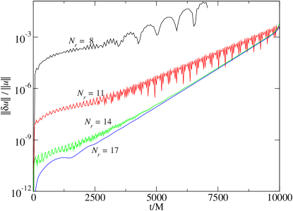
Figure 1: Norm of the error $||\delta u||/||u||$, relative to the reference solution, on a fixed domain extending from minimum coordinate radius $1.9M$ to maximum $41.9M$. The domain is broken into eight shells each of thickness $5M$ and radial resolution $N_{r}$, chosen on four different runs as $N_{r}=8,11,14,17$. The constraint damping terms presented in all of these simulations have $\gamma_{5}=0.6M^{-1}$.

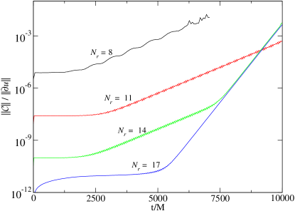
Figure 2: Constraint norm $||{\cal C}||/||\partial u||$, for the same runs plotted in Fig. 1.

As a test of this hypothesis, the highest-resolution run in Fig. 1 was repeated on larger domains, keeping resolution fixed but adding extra subdomains to place the outer boundary at coordinate radii 61.9 $M$, 81.9 $M$, 101.9 $M$. Figure 3 demonstrates the improvement in the overall error norm. Least-squares fitting of the data in that plot show that the late-term growth in this error occurs exponentially on a timescale proportional to the square of the coordinate position of the outer boundary. Figure 4 shows the growth of constraint energy in these simulations. Until an exponential instability sets in, apparently triggered by the overall loss of accuracy of the simulation, the constraint fields grow roughly as the square root of coordinate time. On the largest domain, this slow growth persists beyond 15,000 $M$, when exponential growth takes over at a rate that would allow the simulation to survive until nearly 50,000 $M$.

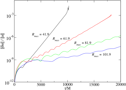
Figure 3: Error norm $||\delta u||/||u||$ for runs in the constraint-damped system with outer boundary at $r=$ 41.9 $M$, 61.9 $M$, 81.9 $M$, 101.9 $M$. The long-term growth of the error norm occurs exponentially on a timescale proportional to the square of the coordinate position of the outer boundary.

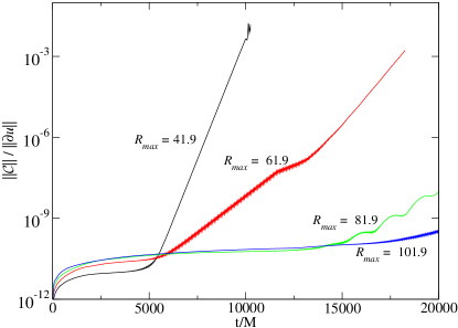
Figure 4: Constraint norm $||{\cal C}||/||\partial u||$ of the same runs as those in Fig. 3. The constraints grow as $t^{1/2}$ until eventually driven exponentially by the overall loss of accuracy demonstrated in Fig. 3.

It is of some interest to verify the effectiveness of the constraint-preserving boundary conditions used in these simulations. As noted in the previous section, since the characteristic matrices of the constraint evolution system are symmetric only with respect to a Lorentzian norm, there is no reason to expect these conditions to control the influx of constraint violations. In Fig. 5, the simulation with $R_{max}=41.9$ and $N_{r}=17$ (in each subdomain) is repeated using conventional boundary conditions. These boundary conditions freeze the incoming characteristic fields of the fundamental evolution system to their initial values. These “freezing” boundary conditions control a positive-definite norm of the fundamental evolution fields, so the initial boundary value problem is known to be well-posed by standard theorems. However, the figure clearly demonstrates the superiority of the constraint-preserving boundary conditions in this context, not only for constraint satisfaction, but for overall stability. Perhaps the effectiveness of the constraint preserving conditions is not robust, perhaps it will fail when the conditions are applied in more dynamical spacetimes. This possibility is an important avenue for further investigation – if this stability is found not to be robust, then either the spatial domain will need to be compactified to remove timelike boundaries, or further modification of the KST system will be needed to combine the constraint damping effects outlined here with truly symmetric hyperbolic constraint propagation.

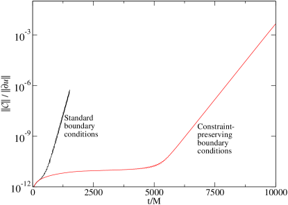
Figure 5: Constraint norm $||{\cal C}||/||\partial u||$ of a black hole simulation with $R_{max}=41.9$, $N_{r}=17$ (in each of eight subdomains), and two different boundary conditions.

VIII Discussion

A generalization of the five-parameter KST systems was introduced, for use in numerical relativity. The added parameter $\gamma_{5}$ supplies a timescale on which exponential damping can occur (or growth, if parameters are not chosen carefully). The hyperbolicity of the fundamental and constraint evolution systems is not changed by this modification, but the effect that the constraint damping has on perturbations of flat spacetime is partly dependent on the same parameters that determine hyperbolicity. Parameters can be chosen such that all constraint modes are stable in perturbations of flat spacetime, but not when the constraint fields are required to evolve in a symmetric-hyperbolic manner. Nevertheless, single black hole simulations using constraint-preserving boundary conditions are convergent, and what instabilities exist appear to be dominated by constraint-satisfying modes, associated with a gauge instability in the outer boundary condition.