A mathematical analysis of the evolution of perturbations in a modified Chaplygin gas model

Abstract

One approach in modern cosmology consists in supposing that dark matter and dark energy are different manifestations of a single ‘quartessential’ fluid. Following such idea, this work presents a study of the evolution of perturbations of density in a flat cosmological model with a modified Chaplygin gas acting as a single component. Our goal is to obtain properties of the model which can be used to distinguish it from another cosmological models which have the same solutions for the general evolution of the scale factor of the universe, without the construction of the power spectrum. Our analytical results, which alone can be used to uniquely characterize the specific model studied in our work, show that the evolution of the density contrast can be seen, at least in one particular case, as composed by a spheroidal wave function. We also present a numerical analysis which clearly indicates as one interesting feature of the model the appearence of peaks in the evolution of the density constrast.

1 Introduction

In an expanding universe distances grow following the expression

$$r\left(t\right)=r_{0}a\left(t\right)\,,$$ (1)

where $a\left(t\right)$ is the scale factor, which indicates how a distance $r$ varies with time, with $r_{0}$ being the present value of $r$. A Taylor’s expansion of such expression around the present time $t_{0}$ produces the approximate relation

$$a\left(t\right)\approx 1+H_{0}\left(t-t_{0}\right)-\frac{1}{2}q_{0}H_{0}^{2}\left(t-t_{0}\right)^{2}\,,$$ (2)

where $a\left(t_{0}\right)=1$, $H_{0}=\left(\dot{a}/a\right)\left|{}_{t=t_{0}}\right.$ and $q_{0}=-\left(\ddot{a}a/\dot{a}^{2}\right)\left|{}_{t=t_{0}}\right.$, with $\dot{a}$ meaning the time derivative of the function $a$. There are several ways of measuring the quantities $H_{0}$ (called Hubble constant) and $q_{0}$ (the decceleration parameter). Presently, the most cited method consists of the observation of supernovae in distant galaxies supernovae1 ; supernovae2 , and its use brought to light the idea that the universe is passing through a phase of accelerated expansion. So, a major problem confronting cosmologists today may be resumed in the question “what causes the acceleration of the universe’s expansion?” Since there are yet no definitive and compelling answers, such issue, named as the problem of dark energy, remains open to debate.

Another parallel puzzle of modern cosmology involves the contradiction between the observed movements of stars in the periphery of galaxies (and of galaxies in clusters of galaxies) and the movements expected from the amount of matter observed directly in such systems. This problem, also noticed when one analyses the data obtained from the cosmic microwave background WMAP , was christened as the problem of dark matter.

Therefore, today’s standard models of cosmology must face the above two problems and, therefore, the models used possess in general five basic components: photons, baryons, neutrinos, dark matter and dark energy. The question “what are dark matter and dark energy?” has, in such models, a standard answer DM : weakly interacting massive particles (WIMPs) combined either to a cosmological constant ($\Lambda$-CDM models) or to some kind of scalar field (quintessence models). Both cosmological constant and a quintessential field could be the source of energy for the acceleration of the universe, while the weakly interacting massive particles, non-luminous, would be responsible for the effect of dark matter.

Another kind of proposal consists in supposing that maybe dark matter and dark energy are in fact different manifestations of a single exotic entity, a component named quartessence (or unified dark matter, UDM) Kamenshchik -quart11 . Quartessential models possess a single fluid whose main characteristic is to present an exotic equation of state $p=p\left(\rho\right)$, which leads to a positive pressure in early phases of the universe and to negative pressures in the late phases. In such context, the main goal of this article is to present a study indicating how density perturbations can evolve in a universe composed solely of a single quartessential fluid. Here, the specific model used is known as the “modified Chaplygin gas” Benaoum –mcg2 . It is very important to notice that solutions for the scale factor obtained in this model may be obtained also in another kinds of cosmological models EueMartin . Therefore, the study of the evolution of perturbations in each one of these models is an important step in the direction of ‘breaking the degeneracy’ between them.

The structure of this work is the following: first, the modified Chapligyn gas model is presented, followed by another section with a brief – and somewhat pedagogical – review of the theory concerning the evolution of perturbations, leading to a differential equation which is used, in sequence, to show how the perturbations evolve in classical single fluid models. In the main section of the article the evolution of perturbations for a modified Chaplygin gas model Sandro is obtained, with conclusions being presented in the last section. Throughout the text natural units are used, where $c=G=\hbar=k_{B}=1$, unless stated otherwise. Also, arbitrary constants present in mathematical solutions are always labeled as $c_{1}$ and $c_{2}$.

2 The modified Chaplygin gas model

The modified Chaplygin gas is characterized by the equation of state

$$p=\left(\gamma-1\right)\rho-M\rho^{-\mu}\,,$$ (3)

where $\gamma$, $M$ and $\mu$ are free parameters. For $\gamma=\mu=1$ one has the original Chaplygin gas, while for $M=0$ one obtains the usual linear equation of state. One must notice that such gas is an ideal fluid, in the sense that it does not present variations in space, ie, $\rho=\rho\left(t\right)$. Therefore, the modified Chaplygin gas model does not incorporate any anisotropic stress, what distinguishes it from some more elaborate models Koivisto .

Using the above equation, together with the condition for conservation of energy in an expanding universe,

$$\dot{\rho}+3\frac{\dot{a}}{a}\left(p+\rho\right)=0\,,$$ (4)

one obtains the relation

$$\rho=\left[\frac{M}{\gamma}+\left(\rho_{0}^{1+\mu}-\frac{M}{\gamma}\right)\left(\frac{a}{a_{0}}\right)^{-3\gamma\left(1+\mu\right)}\right]^{\frac{1}{1+\mu}}\,,$$ (5)

which, when applied in the Friedmann equation,

$$\left(\frac{\dot{a}}{a}\right)^{2}+\frac{k}{a^{2}}=\frac{8\pi}{3}\rho\,,$$ (6)

yields general analytical solutions, valid for any value of the curvature parameter $k$, only for some values of $\gamma$ and $\mu$. For example, for a flat space, Debnath, Banerjee and Chakraborty DBC give the general formula

$$\,{}_{2}F_{1}\left[x,x;1+x;-\frac{M}{\rho_{0}^{1+\mu}\gamma-M}\left(\frac{a}{a_{0}}\right)^{3\gamma\left(1+\mu\right)}\right]=\left(\frac{a}{a_{0}}\right)^{-\frac{3\gamma}{2}}t\sqrt{6\pi}\gamma\left(\rho_{0}^{1+\mu}-\frac{M}{\gamma}\right)^{\frac{1}{2\left(1+\mu\right)}}\,,$$ (7)

where $x=1/\left[2\left(1+\mu\right)\right]$, which can be inverted easily to yield $a=a\left(t\right)$ only for $\mu=0$ and $\mu=-1/2$, while for spaces with any curvature, explicit solutions for $a\left(t\right)$ for the particular choices $\mu=-1/2$, $\gamma=2/3$ and $\gamma=4/3$ are given by Costa Sandro .

It is usual to choose $\mu>0$, but here we will restrict the analysis to the particular choice $\mu=-1/2$, when one has explicitly,

$$p=\left(\gamma-1\right)\rho-M\rho^{1/2}\,,$$ (8)

what gives, for a flat space, where the curvature is null,

$$\rho=\left[\frac{M}{\gamma}+\left(\rho_{0}^{1/2}-\frac{M}{\gamma}\right)\left(\frac{a}{a_{0}}\right)^{-\frac{3\gamma}{2}}\right]^{2}=\frac{3H^{2}}{8\pi}\,,$$ (9)

and, consequently,

$$a\left(t\right)=\lambda\left(e^{\alpha t}-1\right)^{\frac{2}{3\gamma}}\,,$$ (10)

where $\lambda$ is a constant linked to $\gamma$, $M$, $\rho_{0}$ and $a_{0}$, and $\alpha=\sqrt{6\pi M^{2}}$. Therefore, in such model

$$\ddot{a}=\frac{2\lambda}{3\gamma}\alpha^{2}e^{\alpha t}\left(e^{\alpha t}-1\right)^{\frac{2}{3\gamma}-2}\left(\frac{2}{3\gamma}e^{\alpha t}-1\right)\,,$$ (11)

implying that if $e^{\alpha t}>3\gamma/2$ one will have $\ddot{a}>0$. The conclusion is that values of $\gamma$ greater than $2/3$ are more realistic in this model, since then the universe will experience an acceleration on its expansion only in later moments.

Observing equations (8) and (9) and considering the final argument of the previous paragraph, a ‘good’ choice could be $\gamma=4/3$, since in such case the equation of state would interpolate from a phase similar to a radiation dominated universe ($\rho\propto a^{-4}$, for $a<<1$) to a phase with negative pressure, causing the acceleration of the expansion (for $\rho<9M^{2}$), presenting also a phase of pressureless matter (since for values of $\rho\approx 9M^{2}$, one has $p\approx 0$). In resume, then, this particular modified Chaplygin gas model, with $\mu=-1/2$ and $\gamma=4/3$, could, at least in principle, play the role of an effective equation of state for a mixture of radiation, matter and a dynamical cosmological constant.

It is very important to remark that the solution for the scale factor given by eq. (10) (the background solution) can be obtained also in another kinds of flat cosmological models, such as in a decaying vaccum cosmology SauloeAlcaniz . Since an important difference between these two models is on the equation of state used in each one of them, a cosmological test based on properties affected directly by the equation of state could be a potential way to distinguish the models. The analysis of the evolution of perturbations, which has a dependence on the equation of state, is, therefore, a possible way to characterize a model in a way enough to separate it from its concurrents. In the next section, then, we present an overview of the general theory used for describing the evolution of perturbations of density, in order to show the particular relevance of the equation of state in such approach.

3 The theory for the evolution of perturbations

To make a comprehensive overview of the theory concerning the evolution of perturbations in an expanding universe, it is safe to begin with a Newtonian approach, where the radial acceleration $\ddot{R}$ suffered by a test particle previously in equilibrium on the surface of a homogeneous sphere of radius $R$, due to the gravity caused by the increase in the sphere of an excess of mass $\Delta m$, is given by the expression Ryden

$$\ddot{R}=-\frac{G}{R^{2}}\Delta m=-\frac{G}{R^{2}}\left(\frac{4\pi}{3}R^{3}\bar{\rho}\delta\right)\,,$$ (12)

where $\bar{\rho}$ is the mean density of the sphere and $\delta$ is a density fluctuation (known also as density contrast), such that the density inside the sphere is given as $\rho=\bar{\rho}\left(1+\delta\right)$, with $\delta<<1$. The total mass of the sphere is $m=4\pi\bar{\rho}\left(1+\delta\right)/3$, from where one can write, approximately,

$$R\left(t\right)\approx\left(\frac{3m}{4\pi\bar{\rho}}\right)^{1/3}\left[1-\frac{1}{3}\delta\left(t\right)\right]=R_{0}\left[1-\frac{1}{3}\delta\left(t\right)\right]\,.$$ (13)

Using the relations given by equations (12) and (13), and noticing that $R\approx R_{0}$, one can write, then,

$$\frac{\ddot{R}}{R}\approx-\frac{\ddot{\delta}}{3}\,,$$ (14)

and, therefore,

$$\ddot{\delta}=4\pi G\bar{\rho}\delta\,.$$ (15)

This is the equation governing the evolution of density perturbations in a Newtonian static universe. However, if the universe is expanding, one can generalize the above arguments to obtain an equation where the scale factor appears explicitly Ryden ,

$$\ddot{\delta}+2\frac{\dot{a}}{a}\dot{\delta}=4\pi G\bar{\rho}\delta\,.$$ (16)

The procedure leading to a fully general relativistic equation having the density contrast $\delta$ as variable is a more elaborate one. Its development can be traced back to Hawking Hawking , with further advances by Olson Olson and, more recently, by Lyth and Mukherjee Lyth1 , and Lyth and Stewart Lyth2 . A resume of it can be found in a textbook by Padmanabhan Padmanabhan . Here we just cite the final result, which is, explicitly, for a Friedamnn-Lemaître-Robertson-Walker (FLRW) flat universe (where the curvature parameter is zero),

$$\ddot{\delta} + H\left[2-3\left(2w-v^{2}\right)\right]\dot{\delta}-\frac{3}{2}H^{2}\left(1-6v^{2}-3w^{2}+8w\right)\delta=-k^{2}\frac{v^{2}}{a^{2}}\delta\,,$$ (17)

where $H=\dot{a}/a$ is the Hubble parameter, $w=p/\rho$ is the ratio between pressure and energy density of the cosmological fluid, $v^{2}=\frac{\partial p}{\partial\rho}$ is the square of the sound velocity in the fluid, and $k$ is the wavenumber of the Fourier mode of the perturbation. Notice that now one has a dependence on the equation of state $p=p\left(\rho\right)$ of the cosmological fluid in study, included implicitly in the definitions of $\omega$ and $v^{2}$.

To better understand the processes described by these differential equations one can use a purely pragmatic point of view to see whether they can be obtained from effective “Lagrangian densities” where the degrees of freedom are given by $\delta$ and $\dot{\delta}$. From the Lagrangian density

$$\mathcal{L}_{0}=\frac{c^{2}}{G}\left(\frac{\dot{\delta}^{2}}{2}+2\pi G\bar{\rho}\delta^{2}\right)=\frac{1}{2}\left(\frac{c^{2}\dot{\delta}^{2}}{G}\right)+2\pi\bar{\rho}c^{2}\delta^{2}$$ (18)

one produces the Newtonian equation (15), with the constants $c$ and $G$ being used to give the correct dimensionality. In this Lagrangian one has a usual kinetic term, proportional to $\dot{\delta}^{2}$, and a negative potential proportional to $\delta^{2}$, which implies there are no stable points of equilibrium. The solutions, thus, represent only decaying or growing modes.

The result for an expanding universe, eq. (16), can also be obtained by a Lagrangian density

$$\mathcal{L}=\mathcal{L}_{0}a^{2}=\frac{c^{2}}{G}\left(\frac{a^{2}\dot{\delta}^{2}}{2}+\frac{3a^{2}H^{2}\delta^{2}}{4}\right)\,,$$ (19)

with $H^{2}$ standing in the place of $8\pi G\bar{\rho}/3$. Again the potential is negative, but since one has now the kinetic term proportional to $a^{2}\dot{\delta}^{2}$, there is a ‘friction’ in the system.

It is not hard to verify that the general relativistic equation (17), valid for a flat space, can be obtained from a generalization of the above Lagrangians,

$$\mathcal{L}=\frac{\hbar}{c^{3}}\frac{\sqrt{-g}\mathcal{R}}{1+\omega}\frac{a^{2}}{2}\times\left[\dot{\delta}^{2}+\frac{3H^{2}\delta^{2}}{2}\left(1+8\omega-3\omega^{2}-6v^{2}-\frac{2v^{2}k^{2}}{3a^{2}H^{2}}\right)\right]\,,$$ (20)

where $g$ is the determinant of the metric, and $\mathcal{R}=K^{2}-K_{ij}K^{ij}-\,^{3}\mathcal{R}$ is the Ricci scalar built from the extrinsic curvature tensor $K_{ij}$ and the three-curvature $\,{}^{3}\mathcal{R}$ Kolb . For a flat FLRW model $g=-a^{6}$ and $\mathcal{R}=6H^{2}$. Again the potential is proportional to $\delta^{2}$ but it can be positive or negative, according to the value of a polynomial expression involving $\omega$ and $v^{2}$. Therefore, in the general relativistic case one cannot say that all solutions have only growing and decaying modes, since one can have oscillatory behavior. In order to make more clear this point, we present some examples in the next subsection.

3.1 Perturbations in classical models of a single fluid

As commented before, the evolution of perturbations in the general relativistic case can present three distinct possible behaviours: growing, decaying and oscillatory. This can be seen in the simplest models of cosmology, which use a linear equation of state,

$$p=\left(\gamma-1\right)\rho\,,$$ (21)

where $\gamma\neq 0$ is a numerical factor. Such relation, when applied into the energy conservation equation,

$$\dot{\rho}+3H\left(p+\rho\right)=0\,,$$ (22)

and in conjunction with the Friedmann equation for the flat space,

$$H^{2}=\frac{8\pi}{3}\rho\,,$$ (23)

yields, for the scale factor,

$$a\left(t\right)=a_{0}\left(\frac{t}{t_{0}}\right)^{\frac{2}{3\gamma}}\,,$$ (24)

and, consequently,

$$H=\frac{2}{3\gamma}\frac{1}{t}\,.$$ (25)

Using these results into equation (17), one then ends with the equation

$$\ddot{\delta}+\frac{2}{3\gamma t}\left(5-3\gamma\right)\dot{\delta} + \frac{2}{3\gamma^{2}t^{2}}\left(3\gamma^{2}-8\gamma+4\right)\delta=-k^{2}\frac{t_{0}^{\frac{4}{3\gamma}}}{a_{0}^{2}t^{\frac{4}{3\gamma}}}\left(\gamma-1\right)\delta\,.$$ (26)

For any value of $\gamma\neq 0$ this equation has analytical solutions, since it is a particular case of equation 8.491.12 from Gradshteyn and Ryzhik Gradshteyn ,

$$z^{2}u^{\prime\prime}+\left(2\alpha-2\beta\nu+1\right)zu^{\prime}+\left[\beta^{2}\mu^{2}z^{2\beta}+\alpha\left(\alpha-2\beta\nu\right)\right]u=0\,,$$ (27)

with

$$\beta=1-\frac{2}{3\gamma}\,,\,\,\mu^{2}=\frac{k^{2}t_{0}^{\frac{4}{3\gamma}}}{a_{0}^{2}}\left(\gamma-1\right)\left(1-\frac{2}{3\gamma}\right)^{-2}\,,$$

$$\alpha=-1+\frac{2}{\gamma}\,\,\,\mathrm{and}\,\,\,\nu=\left(\frac{1}{2}+\frac{1}{3\gamma}\right)\left(1-\frac{2}{3\gamma}\right)^{-1}$$

or

$$\alpha=-2+\frac{4}{3\gamma}\,\,\,\mathrm{and}\,\,\,\nu=-\left(\frac{1}{2}+\frac{1}{3\gamma}\right)\left(1-\frac{2}{3\gamma}\right)^{-1}\,.$$

3.1.1 Dust matter: $\gamma=1$

In this case the equation to be solved is

$$\ddot{\delta}+\frac{4}{3t}\dot{\delta}-\frac{2}{3t^{2}}\delta=0\,,$$ (28)

with the solution

$$\delta=c_{1}t^{-1}+c_{2}t^{2/3}\,,$$ (29)

where the $c_{i}$ are arbitrary constants. Here, therefore, the solution obtained contains only a growing and a decreasing mode.

3.1.2 Radiation: $\gamma=4/3$

In this case, one has

$$\ddot{\delta}+\frac{1}{2t}\dot{\delta}-\frac{1}{2t^{2}}\delta=-\frac{k^{2}}{3}\frac{t_{0}}{a_{0}^{2}t}\delta\,,$$ (30)

with the oscillatory solution

$$\delta=c_{1}\left(\frac{\sin b_{0}t^{1/2}}{b_{0}t^{1/2}}-\cos b_{0}t^{1/2}\right)+c_{2}\left(\frac{\cos b_{0}t^{1/2}}{b_{0}t^{1/2}}+\sin b_{0}t^{1/2}\right)\,,$$ (31)

where $b_{0}^{2}=4k^{2}t_{0}\left(3a_{0}^{2}\right)^{-1}$ and, again, the $c_{i}$ are arbitrary constants.

4 Evolution of perturbations in the modified Chaplygin gas model

As seen in Section 2, the model we will study is defined by the equation of state (8),

$$p=\left(\gamma-1\right)\rho-M\rho^{1/2}\,,$$

which has two free parameters, $\gamma$ and $M$. In order to verify how the perturbations in the matter density evolve in such model we need to calculate the quantities $\omega=p/\rho$ and $v^{2}=\frac{\partial p}{\partial\rho}$ which appear in equation (17). Therefore, in the model analysed here one has explicitly

$$w=\frac{p}{\rho}=\gamma-1-M\rho^{-1/2}=\gamma-1-\frac{2\alpha}{3H}\,,$$ (32)

$$v^{2}=\frac{\partial p}{\partial\rho}=\gamma-1-\frac{M}{2}\rho^{-1/2}=\gamma-1-\frac{\alpha}{3H}\,.$$ (33)

Substituting the results above in the equation for perturbations, one has

$$\ddot{\delta}+\left[\left(5-3\gamma\right)H+3\alpha\right]\dot{\delta}+\left[\left(3\gamma^{2}-8\gamma+4\right)H^{2}+\left(\frac{22}{3}-4\gamma\right)\alpha H+\frac{4}{3}\alpha^{2}\right]\frac{3\delta}{2}=$$

$$-\frac{k^{2}}{\lambda^{2}}\left(\frac{3\gamma}{2\alpha}H-1\right)^{\frac{4}{3\gamma}}\left(\gamma-1-\frac{\alpha}{3H}\right)\delta\,.$$ (34)

It is easy to notice that this equation simplifies for $\gamma=4/3$. Then, this one will be the choice used in the next subsection. Anyway, one can rewrite the above equation using a new variable, $y=1-\frac{3\gamma H}{2\alpha}=\left(1-e^{\alpha t}\right)^{-1}$, to produce

$$y\left(1-y\right)\frac{d^{2}\delta}{dy^{2}}+\left[\left(\frac{10}{3\gamma}-4\right)y-\frac{10}{3\gamma}\right]\frac{d\delta}{dy}+\left(\frac{2}{1-y}-\frac{6\gamma^{2}-16\gamma+8}{3\gamma^{2}}+\frac{8+6\gamma}{3\gamma^{2}y}\right)\delta=$$

$$-\frac{k^{2}}{\lambda^{2}\alpha^{2}}\left(-y\right)^{\frac{4}{3\gamma}}\left[\left(1-\frac{\gamma}{2}\right)\left(\frac{1}{1-y}+\frac{1}{y}\right)+\frac{\gamma}{2}\frac{1}{\left(1-y\right)^{2}}\right]\delta\,.$$ (35)

For the particular case of the mode with $k=0$, this last equation has a general solution for any value of $\gamma\neq 0$,

$$\delta\left(y\right)=c_{1}\frac{y^{1+\frac{4}{3\gamma}}}{1-y}\,_{2}F_{1}\left(2,1-\frac{2}{3\gamma};2-\frac{2}{3\gamma};y\right)+c_{2}\frac{y^{\frac{2}{\gamma}}}{1-y}\,,$$ (36)

where the $c_{i}$s are arbitrary constants.

4.1 Modified Chaplygin gas model with $\gamma=4/3$

For the particular choice $\gamma=4/3$, equation (4) becomes

$$\ddot{\delta}+\left(H+3\alpha\right)\dot{\delta}-\left(H-2\alpha\right)\left(2H+\alpha\right)\delta=-\frac{k^{2}}{3\lambda^{2}}\left(1-\frac{\alpha}{H}\right)\left(\frac{2H}{\alpha}-1\right)\delta\,.$$ (37)

In the particular case of the mode $k=0$ one has a solution given by eq. (36),

$$\delta\left(t\right)=c_{1}\frac{1-e^{-\alpha t}}{\left(1-e^{\alpha t}\right)^{2}}\,_{2}F_{1}\left(2,\frac{1}{2};\frac{3}{2};\frac{1}{1-e^{\alpha t}}\right)+c_{2}\frac{1-e^{-\alpha t}}{\left(1-e^{\alpha t}\right)^{\frac{3}{2}}}\,.$$ (38)

This solution, which is not oscillatory, can also be written in terms of the Hubble parameter $H$, as

$$\delta\left(H\right)=c_{1}\delta_{1}+c_{2}\delta_{2}\,,$$ (39)

where

$$\delta_{1}=\frac{\left(2H-\alpha\right)^{\frac{3}{2}}}{H}$$ (40)

and

$$\delta_{2}=\frac{\left(2H-\alpha\right)^{2}}{2\alpha H^{2}}+\frac{1}{H}\left(\frac{2H}{\alpha}-1\right)^{\frac{3}{2}}\arctan\left(\frac{2H}{\alpha}-1\right)^{\frac{1}{2}}\,,$$ (41)

and again the $c_{i}$ are arbitrary constants.

4.1.1 Approximate solutions

An approximate solution valid for small values of $t$ can be obtained directly from eq. (37), using that $a\left(t\right)\approx\lambda\alpha^{1/2}t^{1/2}$ and $H\approx t^{-1/2}$, so that the equation to be solved becomes

$$\ddot{\delta}+\left(1+6\alpha t\right)\frac{\dot{\delta}}{2t}+\left(4\alpha^{2}t^{2}+3\alpha t-1\right)\frac{\delta}{2t^{2}}=-\frac{k^{2}}{3\lambda^{2}\alpha t}\left(1-3\alpha t+2\alpha^{2}t^{2}\right)\delta\,,$$ (42)

or, approximately,

$$\ddot{\delta}+\frac{\dot{\delta}}{2t}-\frac{\delta}{2t^{2}}=-\frac{k^{2}}{3\lambda^{2}\alpha t}\delta\,,$$ (43)

which is the equation for a classical model with $\gamma=4/3$, eq. (30), with $\lambda^{2}\alpha$ taking the place of $a_{0}^{2}t_{0}^{-1}$.

In order to obtain an approximate solution valid for large values of $t$ it is interesting to rewrite equation (37) as

$$\ddot{\delta} + \frac{\alpha}{2}\left(7+\frac{1}{e^{\alpha t}-1}\right)\dot{\delta}+\frac{\alpha^{2}}{2}\left[6+\frac{e^{\alpha t}-2}{\left(e^{\alpha t}-1\right)^{2}}\right]\delta=-\frac{k^{2}}{3\lambda^{2}}e^{-\alpha t}\left(\frac{1}{e^{\alpha t}-1}-1\right)\delta\,.$$ (44)

Now, using that $\delta\left(t\right)=e^{-\alpha t}\left(e^{\alpha t}-1\right)^{-1/2}\Gamma\left(t\right)$, the remaining equation is

$$\left(e^{\alpha t}-1\right)\ddot{\Gamma}+\frac{\alpha}{2}\left(e^{\alpha t}-2\right)\dot{\Gamma}=-\frac{k^{2}}{3\lambda^{2}}e^{-\alpha t}\left(2-e^{\alpha t}\right)\Gamma\,,$$ (45)

which, for large values of $\alpha t$, can be approximed to

$$e^{\alpha t}\left(\ddot{\Gamma}+\frac{\alpha}{2}\dot{\Gamma}\right)=\frac{k^{2}}{3\lambda^{2}}\Gamma\,,$$ (46)

with the exact solutions

$$\Gamma\left(t\right)=c_{1}\exp\left[{\frac{2\sqrt{3}}{3}\frac{k}{\lambda\alpha}e^{-\frac{\alpha t}{2}}}\right]+c_{2}\exp\left[{-\frac{2\sqrt{3}}{3}\frac{k}{\lambda\alpha}e^{-\frac{\alpha t}{2}}}\right]\,,$$ (47)

valid for $k\neq 0$, and

$$\Gamma\left(t\right)=c_{1}-c_{2}\frac{2}{\alpha}e^{-\frac{\alpha t}{2}}\,,$$ (48)

valid for $k=0$, where the $c_{i}$ are constants.

Then, summarizing the approximate results for the modes with $k\neq 0$, one has, for $t<<1$,

$$\delta_{t<<1}=c_{1}\left(\frac{\sin bt^{1/2}}{bt^{1/2}}-\cos bt^{1/2}\right)+c_{2}\left(\frac{\cos bt^{1/2}}{bt^{1/2}}+\sin bt^{1/2}\right)\,,$$ (49)

where now $b^{2}=4k^{2}\left(3\lambda^{2}\alpha\right)^{-1}$, while, in the other extreme, for $e^{\alpha t}>>1$,

$$\delta_{t>>1}=c_{1}\exp\left({\frac{2\sqrt{3}}{3}\frac{k}{\lambda\alpha}e^{-\frac{\alpha t}{2}}}-\frac{3\alpha t}{2}\right)+c_{2}\exp\left({-\frac{2\sqrt{3}}{3}\frac{k}{\lambda\alpha}e^{-\frac{\alpha t}{2}}}-\frac{3\alpha t}{2}\right),$$ (50)

with the $c_{i}$ being arbitrary constants.

4.1.2 Solutions in terms of scale factor and conformal time

Although it is more interesting to see the density contrast as a function of the cosmological time $t$, it may be also useful to study its evolution in terms of other variables, such as the conformal time $\eta$ or the scale factor $a$. The Appendix A, at the end of this work, shows such analysis for the classical single fluid models. Since in those models there is a substantial simplification of the differential equations for the density contrast, one can see whether or not this is also the case in the model of a modified Chaplygin gas.

We choose to begin this extra analysis using the scale factor as the independent variable, when the relevant variable transformation is

$$dt=\frac{2a}{\alpha\left(a^{2}+\lambda^{2}\right)}da\,,$$ (51)

and, therefore, the equation to be solved becomes

$$\left(a^{2}+\lambda^{2}\right)\frac{d^{2}\delta}{da^{2}}+8a\frac{d\delta}{da}-\frac{4k^{2}}{3\alpha^{2}}\frac{a^{2}-\lambda^{2}}{\left(a^{2}+\lambda^{2}\right)^{2}}\delta=-2\left(1-\frac{\lambda^{2}}{a^{2}}+\frac{6a^{2}+\lambda^{2}-a^{2}}{a^{2}+\lambda^{2}}\right)\delta\,.$$ (52)

Using the hypothesis

$$\delta=\frac{\lambda^{2}}{a\left(a^{2}+\lambda^{2}\right)}\Gamma$$ (53)

one gets

$$\left(a^{2}+\lambda^{2}\right)\frac{d^{2}\Gamma}{da^{2}}+\frac{2}{a}\left(a^{2}-\lambda^{2}\right)\frac{d\Gamma}{da}=\frac{4k^{2}}{3\alpha^{2}}\frac{a^{2}-\lambda^{2}}{\left(a^{2}+\lambda^{2}\right)^{2}}\Gamma\,,$$ (54)

which for $a\rightarrow 0$ yields

$$\frac{d^{2}\Gamma}{da^{2}}-\frac{2}{a}\frac{d\Gamma}{da}+\frac{4k^{2}}{3\alpha^{2}\lambda^{4}}\Gamma=0\,,$$ (55)

with the solution

$$\Gamma_{a\rightarrow 0}=c_{1}\left(\frac{\sin b_{1}a}{b_{1}}-a\cos b_{1}a\right)+c_{2}\left(\frac{\cos b_{1}a}{b_{1}}+a\sin b_{1}a\right)\,,$$ (56)

where $b_{1}^{2}=4k^{2}/(3\alpha^{2}\lambda^{4})$, while for $a>>\lambda$ one has

$$\frac{d^{2}\Gamma}{da^{2}}+\frac{2}{a}\frac{d\Gamma}{da}-\frac{4k^{2}}{3\alpha^{2}a^{4}}\Gamma=0\,,$$ (57)

with the solution

$$\Gamma_{a>>\lambda}=c_{1}e^{b_{1}\lambda^{2}/a}+c_{2}e^{-b_{1}\lambda^{2}/a}\,.$$ (58)

Finally, for $k=0$ there is an exact solution,

$$\Gamma_{k=0}=c_{1}\left[\frac{1}{2\lambda}\arctan\left(\frac{a}{\lambda}\right)-\frac{a}{2\left(a^{2}+\lambda^{2}\right)}\right]+c_{2}\,.$$ (59)

Therefore, in resume, one has

$$\delta_{a\rightarrow 0}=\frac{c_{1}}{\left(a^{2}+\lambda^{2}\right)}\left(\frac{\sin b_{1}a}{b_{1}a}-\cos b_{1}a\right)+\frac{c_{2}}{\left(a^{2}+\lambda^{2}\right)}\left(\frac{\cos b_{1}a}{b_{1}a}+\sin b_{1}a\right)\,,$$ (60)

$$\delta_{a>>\lambda}=\frac{\lambda^{2}}{a\left(a^{2}+\lambda^{2}\right)}\left[c_{1}e^{b_{1}\lambda^{2}/a}+c_{2}e^{-b_{1}\lambda^{2}/a}\right]\,,$$ (61)

and

$$\delta_{k=0}=c_{1}\left[\frac{\lambda\arctan\left(\frac{a}{\lambda}\right)}{2a\left(a^{2}+\lambda^{2}\right)}-\frac{\lambda^{2}}{2\left(a^{2}+\lambda^{2}\right)^{2}}\right]+c_{2}\frac{\lambda^{2}}{a\left(a^{2}+\lambda^{2}\right)}\,.$$ (62)

We can also present equations for evolution of the perturbations in terms of the conformal time,

$$\eta=\frac{2}{\lambda\alpha}\arccos\left(e^{-\frac{\alpha t}{2}}\right)\,,$$ (63)

so that

$$a=\lambda\tan\left(\frac{\lambda\alpha\eta}{2}\right)\,,$$ (64)

with $0\leq\eta<\frac{\pi}{2}$. With such substitutions equation (54), for example, becomes

$$\frac{d^{2}\Gamma}{d\eta^{2}}-\lambda\alpha\cot\left(\frac{\lambda\alpha\eta}{2}\right)\frac{d\Gamma}{d\eta}=\frac{k^{2}}{3}\left[1-2\cos^{2}\left(\frac{\lambda\alpha\eta}{2}\right)\right]\Gamma\,,$$ (65)

with the solution

$$\Gamma_{k=0}=\frac{c_{1}}{2}\left[\eta-\frac{\sin\left(\lambda\alpha\eta\right)}{\lambda\alpha}\right]+c_{2}\,,$$ (66)

for $k=0$, which is a result completely equivalent to equation (59).

Equation (65) produces a final important result, which can be obtained changing the coordinate to $z=e^{-\frac{\alpha t}{2}}=\cos\left(\frac{\lambda\alpha\eta}{2}\right)$. Doing this, the equation becomes

$$\left(1-z^{2}\right)\frac{d^{2}\Gamma}{dz^{2}}+z\frac{d\Gamma}{dz}=\frac{4k^{2}}{3\lambda^{2}\alpha^{2}}\left(1-2z^{2}\right)\Gamma,$$ (67)

which is a spheroidal wave equation of the type

$$\left(1-z^{2}\right)\frac{d^{2}w}{dz^{2}}-2\left(a+1\right)z\frac{dw}{dz}+\left(b-c^{2}z^{2}\right)w=0\,,$$ (68)

as defined by Stratton Stratton1 ; Stratton2 , with $a=-3/2$, $b=-\frac{4k^{2}}{3\lambda^{2}\alpha^{2}}$ and $c^{2}=-2b$. Solutions to this equation are usually given in terms of elaborate series of special functions or orthogonal polynomials, such as Morse ; Leaver

$$w\left(z\right)=\sum_{n^{\prime}}d_{n}T_{n}^{a}\left(z\right)\,,$$ (69)

where the $d_{n}$’s are the cofficients of the expansion, and $T^{m}_{n}\left(z\right)$ are the Gegenbauer polynomials related to the hypergeometric series $\,{}_{2}F_{1}$ by

$$T^{m}_{n}\left(z\right)=\frac{\left(n+2m\right)!}{2^{m}n!m!}\,_{2}F_{1}\left(n+2m+1,-n;m+1;\frac{1-z}{2}\right)\,.$$ (70)

The series (69) is convergent only for a certain discrete set of values of the quantity $A\equiv b+a+a^{2}$, values which can be obtained from a transcendental equation Abramowitz , and which can be ordered so that for a given $a$, the lowest value of $A$ is labeled $A_{a,a}$, the next is $A_{a,a+1}$, generating an index $\ell$ associated with the solutions through the eigenvalues $A_{a,\ell}<A_{a,\ell+1}$, and so on. The prime on the summation indicates inclusion of only even $n$’s when the quantity $\ell-a$ is even and only odd $n$’s when $\ell-a$ is odd. Various normalization schemes can be used for the $d_{n}$’s, which satisfy a three-order recurrence relation Mathworld .

The subject of spheroidal wave functions is a particularly complex one, and therefore we will, in sequence, resort to numerical methods in order to better visualize the general behaviour of the density perturbations.

4.1.3 Numerical solutions

Besides the analytical solutions presented in this article, we also performed a numerical integration of Eq. (37) in order to analyze the general behavior of the perturbations. The method used for the numerical calculation of the second order differential equation was the finite difference method. The code used for the numerical calculations was tested with the analytical solution obtained with $k=0$, say Eq. (38).

We perform the integration in time of Eq. (37) starting from $t=10^{2}$ years to $t=1.2\times 10^{11}$ years. The approximate solution (49) was used to apply the initial conditions of our problem. The numerical results show clearly the presence of a peak in the evolution of the perturbations for any value of $k$. Results for some values of the wavenumber $k$ are depicted in Fig. 1. The integral path used in Fig. 1 was $\Delta t=1$ year. Numerical simulations with less acuracy, $\Delta t>1$ year, show that the time in which the peak is maximum is practically the same but some details on the perturbation profiles are lost. Note that the maximum value of the perturbation increases when we increase the wavenumber value. The time in which the perturbation value is maximum also depends on the value of $k$. This behaviour is depicted in Fig. 2. The numerical results of Fig. 2 were obtained with a integration path of $\Delta t=10^{3}$ years to save integration time. All figures were built with the values $\alpha=1.28\times 10^{-10}$ years^-1, $t_{0}=1.4\times 10^{10}$ years and $a_{0}=a\left(t_{0}\right)=1$.

Figure 1: Graph showing the general behaviour of perturbations in a modified Chapligyn gas with $\gamma=4/3$ for two values of the wavenumber $k$. Here, it is clear the presence of peaks. The scale in the vertical axis is arbitrary. Numerical results for other wavenumber values present similar behaviours.

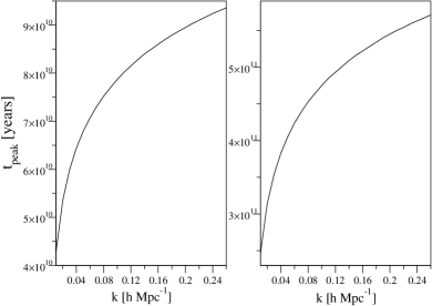
Figure 2: Graphs presenting the dependence of the time in which the perturbation is maximal, $t_{peak}$, with the wavenumber of the perturbation, $k$, for $\gamma=4/3$ (left) and $\gamma=2/3$ (right).

4.2 Modified Chaplygin gas with $\gamma\neq 4/3$

Another values of $\gamma$ different of $4/3$ allow one to obtain some analytical and numerical results, using procedures analogous to the one used for $\gamma=4/3$. Starting from equation (4) or (4), using as variable the scale factor $a$, and putting

$$\delta=\frac{\left(-1\right)^{\frac{2}{\gamma}}\left(\frac{\lambda}{a}\right)^{3}}{1+\left(\frac{\lambda}{a}\right)^{\frac{3\gamma}{2}}}\Gamma\,,$$ (71)

one obtains

$$\left[1+\left(\frac{a}{\lambda}\right)^{\frac{3\gamma}{2}}\right]\frac{d^{2}\Gamma}{da^{2}}-\frac{3\gamma}{2a}\left[1-\left(\frac{a}{\lambda}\right)^{\frac{3\gamma}{2}}\right]\frac{d\Gamma}{da}=-\frac{9\gamma^{2}k^{2}}{4\alpha^{2}a^{4}}\left\{\frac{\gamma}{2}\frac{\left(\frac{a}{\lambda}\right)^{3\gamma}}{\left[1+\left(\frac{a}{\lambda}\right)^{\frac{3\gamma}{2}}\right]^{2}}-\left(1-\frac{\gamma}{2}\right)\frac{\left(\frac{a}{\lambda}\right)^{3\gamma}}{1+\left(\frac{a}{\lambda}\right)^{\frac{3\gamma}{2}}}\right\}\Gamma\,.$$

As a first example, for $\gamma=2/3$ one has then

$$\left(a+\lambda\right)\frac{d^{2}\Gamma}{da^{2}}+\left(a-\lambda\right)\frac{1}{a}\frac{d\Gamma}{da}=-\frac{k^{2}\lambda}{3\alpha^{2}a^{2}}\left[\frac{1}{\left(a+\lambda\right)^{2}}-\frac{2}{\lambda\left(a+\lambda\right)}\right]\Gamma\,,$$ (73)

which for $a\rightarrow 0$ reduces to

$$\frac{d^{2}\Gamma}{da^{2}}-\frac{1}{a}\frac{d\Gamma}{da}-\frac{k^{2}}{3\alpha^{2}\lambda^{2}}\frac{\Gamma}{a^{2}}=0\,,$$ (74)

with the solution

$$\Gamma_{a\rightarrow 0}=a\left[c_{1}a^{\sqrt{1+\frac{k^{2}}{3\alpha^{2}\lambda^{2}}}}+c_{2}a^{-\sqrt{1+\frac{k^{2}}{3\alpha^{2}\lambda^{2}}}}\right]\,,$$ (75)

while for $a>>\lambda$ one has

$$\frac{d^{2}\Gamma}{da^{2}}+\frac{1}{a}\frac{d\Gamma}{da}-\frac{2k^{2}}{3\alpha^{2}}\frac{\Gamma}{a^{4}}=0\,,$$ (76)

with the solution

$$\Gamma_{a>>\lambda}=c_{1}K_{0}\left(\sqrt{\frac{2k^{2}}{3\alpha^{2}}}\frac{1}{a}\right)+c_{2}I_{0}\left(\sqrt{\frac{2k^{2}}{3\alpha^{2}}}\frac{1}{a}\right)\,.$$ (77)

As another example, one can use $\gamma=2$ to obtain the equation

$$\left(a^{3}+\lambda^{3}\right)\frac{d^{2}\Gamma}{da^{2}}+\frac{3}{a}\left(a^{3}-\lambda^{3}\right)\frac{d\Gamma}{da}=-\frac{9k^{2}\lambda^{3}}{\alpha^{2}}\frac{a^{2}}{\left(a^{3}+\lambda^{3}\right)^{2}}\Gamma\,.$$ (78)

When $a\rightarrow 0$ such equation becomes

$$\frac{d^{2}\Gamma}{da^{2}}-\frac{3}{a}\frac{d\Gamma}{da}+\frac{9k^{2}}{\alpha^{2}\lambda^{6}}a^{2}\Gamma=0\,,$$ (79)

which has the solution

$$\Gamma_{a\rightarrow 0}=a^{2}\left[c_{1}J_{1}\left(\frac{3k}{2\alpha\lambda^{3}}a^{2}\right)+c_{2}J_{-1}\left(\frac{3k}{2\alpha\lambda^{3}}a^{2}\right)\right]\,,$$ (80)

while for $a>>\lambda$ one has

$$\frac{d^{2}\Gamma}{da^{2}}+\frac{3}{a}\frac{d\Gamma}{da}+\frac{9k^{2}\lambda^{3}}{\alpha^{2}}\frac{\Gamma}{a^{7}}=0\,,$$ (81)

which has the solution

$$\Gamma_{a>>\lambda}=a^{-1}\left[c_{1}J_{\frac{2}{5}}\left(\frac{6k\lambda^{\frac{3}{2}}}{5\alpha}a^{-\frac{5}{2}}\right)+c_{2}J_{-\frac{2}{5}}\left(\frac{6k\lambda^{\frac{3}{2}}}{5\alpha}a^{-\frac{5}{2}}\right)\right]\,.$$ (82)

As numerical example, we choose the value $\gamma=5/3$ and, following the procedures presented for $\gamma=4/3$, we obtained the graphs presented in Fig. 3, which represent well the kinds of behaviours we encountered in our computations for several values of $\gamma$.

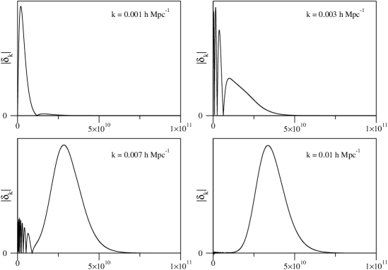
Figure 3: Graphs presenting the behaviour of the modulus of the density contrast, $\left|\delta_{k}\right|$, with the time $t$ (in years), for some values of the wavenumber of the perturbation, $k$, for $\gamma=5/3$. Notice the presence of oscillations in the early times, along with the formation of a peak. The vertical scale is arbitrary in all graphs. Also, in all graphs the integral path used was $\Delta t=10^{2}$ years.

We also made, now for $\gamma=2/3$, a numerical calculation of the time $t_{peak}$ in which the maximum value of the peak is attained for each mode with wavenumber $k$, and such calculations are presented in Fig. 2.

5 Final remarks

In this work, we present the mathematical analysis of the evolution of density perturbations in a flat cosmological model with a modified Chaplygin gas acting as a single component, in order to verify whether this kind of analysis can be used to distinguish such class of models from another cosmological models which have the same solutions for the general evolution of the scale factor of the universe. For example, the solution

$$a\left(t\right)=\lambda\left(e^{\alpha t}-1\right)^{1/2}\,,$$ (83)

shown here, can also be obtained in models with a constant bulk viscosity or with a decaying $\Lambda$-term of the type $\Lambda=\sigma H$ EueMartin . Our goal was to verify to what degree such degeneracy between models could be broken from the theory alone, without resorting to observational data. And our work shows that the analysis of the evolution of perturbations can be sufficient, since it produces results which can characterize uniquely a model such as the modified Chaplygin gas. As an example of this, we can point that a preliminary analysis of the evolution of perturbations in the $\Lambda$-decaying model for the mode $k=0$ Saulopersonal indicates a result completely diferent from the one given by equation (36).

It is also important to notice that we have shown it is possible to find a complete analytical solution for the evolution of the density contrast, involving spheroidal functions and the conformal time $\eta$, in the particular model studied by us, i.e., a modified Chaplygin gas model described by the equation of state,

$$p=\left(\gamma-1\right)\rho-M\rho^{-\mu}\,,$$ (84)

with $\gamma=4/3$ and $\mu=-1/2$. It is very unlikely that other classes of models present the same kind of solution and, as a matter of fact, it is very unlikely also that other Chaplygin gas models, with values of $\gamma$ and $\mu$ different from the ones chosen by us, will lead to analytical solutions. However, it is certain that the analytical solutions we found, although limited to a specific choice of parameters in a model, can be useful to test numerical codes, to provide some insight for more generic numerical solutions, and by themselves are interesting for pedagogical purposes.

Another relevant point to be noticed in our work is that our numerical analysis, together with the analytical approximate solutions obtained, shows that the density perturbation has peaks in its evolution. Furthermore, the time in which the peak is maximum depends on the value of the wavenumber $k$. Also, the perturbation magnitude is very sensitive to the value of $k$. These properties may characterize the modified Chaplygin model and help to distinguish it from other models.

To finish, we must emphasize that a thorough analysis of the evolution of perturbations in a particular model must include the power spectrum, in order to allow a fair evaluation of the possible validity of the model. Here, our intention was to show that the results obtained for a specific choice of the parameters of the modified Chaplygin gas are enough to allow the distinction from another models, from a purely mathematical point of view, i.e., even without the construction of the power spectrum. Therefore, a comparison of the power spectrum predicted by this model and the one observed remains as a point to be attacked in future works.

Appendix A Other forms of the equation for perturbations

An interesting alternative form of writing the differential equation which describes the evolution of the perturbations in the general relativistic context, eq. (17), is obtained using the scale factor $a$ as the variable, i.e. (cf. equation 4.122 from Padmanabhan Padmanabhan ),

$$\frac{d^{2}\delta}{da^{2}}+\frac{1}{2a}\frac{d\delta}{da}\left(3-15\omega+6v^{2}\right)-\frac{3\delta}{2a^{2}}\left(1-6v^{2}-3\omega^{2}+8\omega\right)=-\frac{k^{2}v^{2}}{H^{2}a^{4}}\delta\,.$$ (85)

Such result can also be written as

$$\frac{d^{2}\delta}{d\eta^{2}}+\mathcal{H}\left[1-3\left(2\omega-v^{2}\right)\right]\frac{d\delta}{d\eta}-\mathcal{H}^{2}\left(1-6v^{2}-3\omega^{2}+8\omega\right)\frac{3\delta}{2}=-k^{2}v^{2}\delta\,,$$ (86)

where $\eta$ is the conformal time defined by the relation $dt=ad\eta$, and

$$\mathcal{H}=\frac{1}{a}\frac{da}{d\eta}\,.$$ (87)

For classical models of a single fluid in a flat space, with $\gamma\neq 2/3$, one has

$$a\left(\eta\right)=a_{0}\left(\frac{\eta}{\eta_{0}}\right)^{\frac{2}{3\gamma-2}}\,,$$ (88)

where $\eta_{0}$ is a constant, and

$$\mathcal{H}\left(\eta\right)=\frac{2}{3\gamma-2}\frac{1}{\eta}\,,$$ (89)

so that the equation obeyed by the perturbations is

$$\frac{d^{2}\delta}{d\eta^{2}}-\left(\frac{\gamma-\frac{4}{3}}{\gamma-\frac{2}{3}}\right)\frac{2}{\eta}\frac{d\delta}{d\eta}+\left(\frac{\gamma-2}{\gamma-\frac{2}{3}}\right)\frac{2\delta}{\eta^{2}}=-k^{2}\left(\gamma-1\right)\delta\,,$$ (90)

from where it is easy to see the simplicity of three particular cases ($\gamma=1,4/3$ and $2$) and which has a general solution in terms of Bessel functions,

$$\delta\left(\eta\right)=\eta^{\frac{1}{2}\frac{9\gamma-10}{3\gamma-2}}J_{\pm\frac{1}{2}\frac{3\gamma+2}{3\gamma-2}}\left(\eta k\sqrt{\gamma-1}\right)\,.$$ (91)

On the other hand, using $a$ as variable one has the equation

$$\frac{d^{2}\delta}{da^{2}}-\frac{9}{2a}\left(\gamma-\frac{4}{3}\right)\frac{d\delta}{da}+\left(\gamma-2\right)\left(\gamma-\frac{2}{3}\right)\frac{9\delta}{2a^{2}}=-\frac{k^{2}}{a^{4-3\gamma}}\left(\frac{3}{8\pi\rho_{0}a_{0}^{3\gamma}}\right)\left(\gamma-1\right)\delta\,,$$ (92)

which also can be solved with Bessel functions,

$$\delta\left(a\right)=a^{\frac{9\gamma-10}{4}}J_{\pm\frac{1}{2}\frac{3\gamma+2}{3\gamma-2}}\left[\frac{3k}{3\gamma-2}\left(\frac{\gamma-1}{6\pi\rho_{0}a_{0}^{3\gamma}}\right)^{\frac{1}{2}}a^{\frac{3\gamma-2}{2}}\right]\,,$$ (93)

and from where it is easy also to see the simplification which can be obtained for some particular values of $\gamma$.

References

- (1) Perlmutter, S. et al.: Astrophys. J. 517, 565 (1999)
- (2) Riess, A.G. et al.: Astronomical J. 116, 1009 (1998)
- (3) Bennett, C.L. et al: Astrophys. J. Suppl. 148, 1 (2003)
- (4) Turner, M.S.: The Sciences 40, 32 (2000)
- (5) Kamenshchik, A., Moschella, U., Pasquier, V.: Phys. Lett. B 511, 265 (2001)
- (6) Bento, M.C., Bertolami, O., Sen, A.A.: Phys. Rev. D 66, 043507 (2002)
- (7) Bento, M.C., Bertolami, O., Sen, A.A.: Phys. Rev. D 70, 083519 (2004)
- (8) Makler, M., Oliveira, S.Q., Waga, I.: Phys. Lett. B 555, 1 (2003)
- (9) Ananda, K.N., Bruni, M.: Phys. Rev. D 74, 023523 (2006)
- (10) Ananda, K.N., Bruni, M.: Phys. Rev. D 74, 023524 (2006)
- (11) Diez-Tejedor, A., Feinstein, A.: Phys. Rev. D 74, 023530 (2006)
- (12) Giannakis, D., Hu, W.: Phys. Rev. D 72, 063502 (2005)
- (13) Perrota, F., Matarrese, S., Torki, M.: Phys. Rev. D 70, 121304 (2004)
- (14) Gorini, V. et al: Phys. Rev. D 72, 103518 (2005)
- (15) Carturan, D., Finelli, F.: Phys. Rev. D 68, 103501 (2003)
- (16) Zhu, Z.H.: Astron. Astrophys. 423, 421 (2004)
- (17) Sandvik, H.B. et al: Phys. Rev. D 69, 123524 (2004)
- (18) Scherrer, R.J.: Phys. Rev. Letters 93, 011301 (2004)
- (19) Dev, A., Jain D., Alcaniz, J.S.: Astron. Astrophys. 417, 847 (2004)
- (20) Avelino, P.P. et al: Phys. Rev. D 69, 041301 (2004)
- (21) Amendola, L. et al: Journal of Cosmology and Astroparticle Physics 7, 005 (2003)
- (22) Beca, L.M.G. et al: Phys. Rev. D 67, 101301 (2003)
- (23) Velasquez-Toribio, A.M.: Braz. J. Phys. 36, 772 (2006)
- (24) Amendola, L. et al: Phys. Rev. D 74, 063524 (2006)
- (25) Amendola, L., Waga, I., Finelli, F.: Journal of Cosmology and Astroparticle Physics 11, 009 (2005)
- (26) Colistete, R., Fabris, J.C.: Class. Quantum Grav. 22, 2813 (2005)
- (27) Reis, R.R.R., Makler, M., Waga, I.: Class. Quantum Grav. 22, 1191 (2005)
- (28) Reis, R.R.R., Makler, M., Waga, I.: Class. Quantum Grav. 22, 353 (2005)
- (29) Reis, R.R.R., Makler, M., Waga, I.: Phys. Rev. D 69, 101301 (2004)
- (30) Avelino, P.P et al: Phys. Rev. D 69, 041301 (2004)
- (31) Makler, M., de Oliveira, S.Q., Waga, I.: Phys. Rev. D 68, 123521 (2003)
- (32) Reis, R.R.R. et al: Phys. Rev. D 68, 061302 (2003)
- (33) Benaoum, H.B.: hep-th/0205140 (2005)
- (34) Debnath, U., Banerjee, A., Chakraborty, S.: Class. Quantum Grav. 21, 5609 (2004)
- (35) Chimento, L.P.: Phys. Rev. D 69, 123517 (2004)
- (36) Barreiro, T., Sen, A.A.: Phys. Rev. D 70, 124013 (2004)
- (37) Costa, S.S., Makler, M.: astro-ph/0702418 (2007)
- (38) Costa, S.S.: Braz. J. Phys. 35, 1046 (2005)
- (39) Koivisto, T., Mota, D.F.: Phys. Rev. D 73, 083502 (2006)
- (40) Carneiro, S., Pigozzo, C., Borges, H.A., Alcaniz, J.S.: Phys. Rev. D 74, 023532 (2006)
- (41) Ryden, B.: Introduction to cosmology, Addison-Wesley (2003)
- (42) Hawking, S.W.: Astrophys. J. 145, 544 (1966)
- (43) Olson, D.W.: Phys. Rev. D 14, 327 (1976)
- (44) Lyth, D.H., Mukherjee, M.: Phys. Rev. D 38, 485 (1988)
- (45) Lyth, D.H., Stewart, E.D.: Astrophys. J. 361, 343 (1990)
- (46) Padmanabhan, T.: Structure formation in the universe, Cambridge Universe Press (1993)
- (47) Kolb, E.W., Turner, M.S.: The early universe, Addison-Wesley (1993)
- (48) Gradshteyn, I.S., Ryzhik, I.M.: Table of Integrals, Series and Products, Academic Press (2000)
- (49) Stratton, J.A.: Proc. Nat. Acad. Sci. 21, 51 (1935)
- (50) Stratton, J.A.: Proc. Nat. Acad. Sci. 21, 316 (1935)
- (51) Morse, P.M., Feshbach, H.: Methods of Theoretical Physics, McGraw-Hill (1953)
- (52) Leaver, E.W.: J. Math. Phys. 27, 1238 (1986)
- (53) Abramowitz, M., Stegun, I.A.: Handbook of Mathematical Functions with Formulas, Graphs, and Mathematical Tables, Dover (1972)
- (54) Weisstein, E.W.: Prolate Spheroidal Function, MathWorld – A Wolfram Resource. http:// mathworld.wolfram.com/ProlateSpheroidalWaveFunction.html
- (55) Carneiro, S.: Modelo cosmológico com decaimento do vácuo – novos resultados e limites observacionais, talk presented at the VI Workshop Nova Física no Espaço (2007).