An Evidence Based Search Method For Gravitational Waves From Neutron Star Ring-downs

Abstract

The excitation of quadrupolar quasi-normal modes in a neutron star leads to the emission of a short, distinctive, burst of gravitational radiation in the form of a decaying sinusoid or ‘ring-down’. We present a Bayesian analysis method which incorporates relevant prior information about the source and known instrumental artifacts to conduct a robust search for the gravitational wave emission associated with pulsar glitches and soft $\gamma$-ray repeater flares. Instrumental transients are modelled as sine-Gaussian and their evidence, or marginal likelihood, is compared with that of Gaussian white noise and ring-downs via the ‘odds-ratio’. Tests using simulated data with a noise spectral density similar to the LIGO interferometer around $1$ kHz yield $50\%$ detection efficiency and $1\%$ false alarm probability for ring-down signals with signal-to-noise ratio $\rho=5.2$. For a source at $15$ kpc this requires an energy of $1.3\times 10^{-5}M_{\astrosun}c^{2}$ to be emitted as gravitational waves.

I Introduction

A possible mechanism for the emission of gravitational waves from neutron stars is the excitation of non-radial quasi-normal modes (QNMs) Thorne (1969). This excitation could be caused by the disruption associated with pulsar glitches Kokkotas et al. (2001) or from flaring activity in soft $\gamma$-ray repeaters de Freitas Pacheco (1998).

The frequencies and damping times of the QNMs depend strongly on the neutron star equation of state (EOS) and for the more dominant f-modes these are thought to lie somewhere in the region of $1$ to $4$ kHz and $50$ to $500$ ms, respectively. Andersson & Kokkotas Andersson and Kokkotas (1998) have shown how the mass and radius of a neutron star may be constrained by gravitational wave observations of the QNM frequencies and decay times. Conversely, if the EOS of the neutron star were known with some precision, it would be possible to compute the expected decay times and frequencies of the QNMs. This would provide a well constrained waveform model for aiding the identification of a potential gravitational wave signal following a neutron star ring-down. However, the behaviour of matter at the densities found in neutron stars is not well understood and there exist many different models for the neutron star EOS. It is, therefore, necessary to develop techniques which are robust to the uncertainties in these models.

While the gravitational wave emission from neutron star QNMs is expected to be weak (inducing typical strain amplitudes of $\sim 10^{-24}$), their detection is further hampered by the presence of instrumental glitches that can closely resemble short-duration gravitational wave signals.

In this work, we demonstrate the feasibility of applying Bayesian inference to the robust detection of neutron star gravitational wave ring-downs through a process of model selection. We highlight how the methodology may be extended to include a more realistic range of glitches and developed into a multi-detector search.

II Perturbed neutron stars & asteroseismology

When the solid crust of a neutron star is severely disrupted or cracked, some of the stored elastic energy is channeled into the oscillatory modes of the star. Quadrupolar excitations will then be strongly damped by gravitational wave emission Thorne (1969). The different modes may be labelled according to the spherical harmonic indices $l$ and $m$ which describe the angular dependence and number of nodes.

The fundamental fluid mode, or $f$-mode (as first shown by Kelvin for the case of a non-rotating, uniform density star) has angular frequency

$$\omega_{f}^{2}=\frac{2l(l-1)}{2l+1}\frac{GM}{R^{3}},$$ (1)

where $M$ and $R$ are the stellar mass and radius, respectively. This is also a reasonable estimate for more realistic equations of state Andersson (2003) and we see that, for non-radial modes with $l=2$, the $f$-mode pulsations have frequencies $\sim 2$ kHz taking the fiducial values $M=1.4M_{\astrosun}$ and $R=10$ km. Other modes, such as the pressure ($p$) and space-time ($w$) modes, have considerably higher frequencies than this. Gravitational wave interferometers like GEO600 Lück et al. (2006), LIGO Sigg (2006) (for the LIGO Science Collaboration) and VIRGO Tournefier and VIRGO Collaboration (2005) are more sensitive at lower frequencies making the $f$-mode the most favourable for a gravitational wave search. The ring-down timescale, $\tau_{f}$, is given by the ratio of the oscillation energy to the total power emitted as gravitational waves Andersson and Kokkotas (1998). This yields $\tau_{f}\sim R(R/M)^{3}$, where $M$ and $R$ are the mass and radius of the neutron star, respectively.

So, given some EOS, which defines the ratio $M/R$, it is possible to calculate the exact damping times and frequencies of the QNMs. Andersson & Kokkotas Andersson and Kokkotas (1998) do precisely this for a variety of equations of state and establish empirical relations for the $f$-mode damping time and frequency. On the other hand, we can consider the inverse problem and use gravitational wave observations of the $f$-mode frequency and damping time to constrain the neutron star EOS. Indeed, there has already been an attempt to use the electromagnetically observed frequencies of potential torsional mode oscillations in two SGRs to constrain their equations of state Samuelsson and Andersson (2007).

Here, our interest is in using what little is known about the neutron star equation of state to inform us with regards to sensible gravitational wave waveforms to search for. Fig. 1 shows the results of calculations by Benhar et al Benhar et al. (2004) of the $f$-mode frequency and damping time, using several realistic EOSs and the extremal neutron star masses. $\rm M_{\rm max}$ refers to the maximum neutron star mass allowed by the EOS. The reader is directed to Benhar et al. (2004) and the references therein for descriptions of the different equations of state.

Figure 1: The f-mode frequencies & damping times for the variety of different equations of state (indicated by symbol shape) and the extremal neutron star masses (indicated by symbol weight) considered in Benhar et al. (2004).

Examining Fig. 1 we see that the equations of state considered in Benhar et al. (2004) yield typical $f$-mode frequencies of $\nu_{f}\sim 1.5-3$ kHz and damping timescales of $\tau_{f}\sim 50-400$ ms. Later, we use these ranges to set sensible limits of our priors for each parameter.

Gravitational wave emission

Following Thorne Thorne (1969), we model the gravitational wave strain amplitude at the Earth from the $n$-th QNM as:

$$h(t)=\left\{\begin{tabular}[]{cl}$h_{0}\sin\left[\omega_{n}\left(t-t_{0}\right)\right]e^{\left[-\frac{(t-t_{0})}{\tau_{n}}\right]}$&for $t\geq t_{0}$\\ \\ $0$&otherwise, $$\\ \end{tabular}\right.$$

(2)

where $h_{0}$, $\omega_{n}$ and $\tau_{n}$ are the initial amplitude, angular frequency and characteristic damping time of the signal, and $t_{0}$ is the start time of the signal. We take $n=0$ to represent the $f$-mode.

Furthermore, $h_{0}$, $\omega_{0}$ and $\tau$ are related to the total gravitational wave energy via the following relation de Freitas Pacheco (1998),

$$E_{\textrm{\scriptsize{GW}}}=\frac{c^{3}D^{2}}{4G}\left(h_{0}\omega_{0}\tau^{\frac{1}{2}}\right)^{2},$$ (3)

where $D$ is the distance to the source. We can, therefore, write down an expression for the the expected initial amplitude for $f$-mode ring-downs using fiducial parameter values:

$$h_{0}\sim 1.6\times 10^{-24}\left(\frac{E_{\textrm{\scriptsize{GW}}}}{10^{-11}M_{\astrosun}c^{2}}\right)^{1/2}\left(\frac{\tau}{200\ \textrm{ms}}\right)^{-1/2}\left(\frac{\nu_{0}}{2\ \textrm{kHz}}\right)^{-1}\left(\frac{D}{15\ \textrm{kpc}}\right)^{-1}.$$ (4)

Search triggers & QNM excitation

There are several ways to generate stellar pulsations including close encounters with orbital companions and accretion (e.g., of comets), the ringing of proto-neutron stars following supernovae, soft $\gamma$-ray repeater (SGR) flaring activity and crustal disruption due to pulsar glitches.

Our aim is to search for gravitational waves from the latter two mechanisms. This is because both pulsar glitches and the SGRs provide an observable electromagnetic counterpart (which may be used to ‘trigger’ the search) and occur with a frequency making them practical for a triggered search. The most prolifically glitching pulsar, PSR J0537-6910, has a glitch rate of $\sim 4\,{\rm year}^{-1}$ Middleditch et al. (2006), whilst other regular glitchers like the Crab pulsar and Vela have rates of order $\sim 0.5\,{\rm year}^{-1}$ Cra ; Dodson et al. (2006). SGRs are seen to emit bursts at rates of a few to $10\,{\rm year}^{-1}$ Nakagawa et al. (2007), whereas hyperflares are much rarer events occuring maybe once a decade. Other potential candidates seen to glitch are the anomalous X-ray pulsars (AXPs).

Pulsar glitches

Pulsar glitches are observed as sudden irregularities in the rotation rate of pulsars and are characterised by a step increase in rotation frequency. The characteristics of glitches vary between pulsars. For example, some show step changes in the spin-down rate and others exponential recoveries to pre-glitch parameters. The exact characteristics give clues to the underlying mechanisms causing the glitch.

The mechanisms responsible for pulsar glitches are still unclear, but there are two main candidates to explain the underlying process and some of the differences between glitches. For older pulsars it seems glitches are likely caused by a dramatic decoupling between the star’s solid crust and superfluid interior Cheng et al. (1988). Glitches in the young Crab pulsar are thought to be associated with a reconfiguration of the solid crust Franco et al. (2000): the spin-down reduces the centrifugal force and the crust reaches breaking strain. The ensuing relaxation of ellipticity will cause a sudden change in the moment of inertia, producing the observed glitch, and the crustal rupture will set up a starquake, hopefully causing $f$-mode excitations. The reality of the mechanism is likely to be very complex and may be a combination of the two.

For the two different glitch models the amount of energy released can be estimated in different ways as shown in van Riper et al. (1991) van Riper et al. (1991). They assume all the energy released goes into heating the star, whereas we will make the assumption that it goes into exciting quasi-normal modes. For the angular momentum exchange model (thought to be the most probable explanation for the Vela pulsar glitches) the amount of energy released depends on the angular momentum exchanged between the superfluid interior and crust $\Delta{}J\sim I\Delta\Omega$, where $\Delta\Omega$ is the angular frequency change from the glitch. The energy change is then $\Delta{}E=\Delta{}J\Omega_{\rm lag}$, where $\Omega_{\rm lag}$ is the lag frequency between the superfluid and crust, with an estimated range of values of 1-100 rad ${\rm s}^{-1}$ (or possibly $\lesssim 0.1$ rad ${\rm s}^{-1}$) van Riper et al. (1991). For the largest Vela pulsar glitch, with a fractional frequency change of $\Delta\Omega/\Omega=3.1\!\times\!10^{-6}$ Dodson et al. (2002), this gives a $\Delta{}J\sim 2\!\times\!10^{34}$ J giving an energy release of $\Delta{}E\sim 10^{-13}-10^{-11}\,{\rm M}_{\odot}c^{2}$ for the range $\Omega_{\rm lag}\approx$ 1-100 rad ${\rm s}^{-1}$.

For starquake driven glitches the energy released is given in Ref. van Riper et al. (1991) as $\Delta{}E\approx\mu{}V_{\rm crust}\epsilon_{\rm max}\epsilon_{\rm quake}$, where $\epsilon_{\rm quake}=\Delta\Omega/\Omega$ is equivalent to the relative change in moment of inertia, $\mu$ is the mean shear modulus of the star, $V_{\rm crust}$ is the volume of the crust (where $\mu{}V_{\rm crust}\sim 10^{41}$ J), and $\epsilon_{\rm max}$ is the maximum deformation from equilibrium the crust can withstand without breaking (given in Ref. van Riper et al. (1991) as $\epsilon_{\rm max}\lesssim 10^{-2}$ although this could vary somewhat). Assuming this $\epsilon_{\rm max}$ and taking the largest Crab pulsar glitch, where $\Delta\Omega/\Omega\sim 8\!\times\!10^{-8}$ Lyne et al. (1993), we get an energy release of $\Delta{}E\sim 5\!\times\!10^{-16}\,{\rm M}_{\odot}c^{2}$. If the starquake mechanism can provide similar fractional frequency changes to a neutron star to those seen in the Vela pulsar during glitches, then this mechanism could still be a valuable potential source.

Soft $\gamma$-ray repeater flares

Soft $\gamma$-ray repeaters are high energy transient sources with typical photon energies of $10-30$ keV and similar burst characteristics from one event to the next, although they are also seen as quiescent X-ray sources. These objects are identified as highly magnetised ($B\approx 10^{14}$ Gauss) neutron stars, or ‘magnetars’. They are occasionally seen to emit giant flares, or hyper-flares, which have thousands of times the luminosity, and harder spectra, than the regular bursts. The hyperflares are thought to occur when magnetic field becomes twisted and causes a catastrophic reconnection, inducing tectonic activity. The field annihilation/reconnection in seismic faults is responsible for the observed $\gamma$-ray emission and, again, we expect the crustal disruption to excite the QNMs of the magnetar Hurley et al. (2005).

III Bayesian Model Selection

Before moving on to describe the search in detail, we outline some ideas behind Bayesian model selection.

Bayes’ theorem describes how to assign a posterior probability to some parameterised model $M_{i}$, given a set of data or observations $D$ and some background information $I$ which determines the hypothesis space $\{M_{i}\}$:

$$p(M_{i}|D,I)=\frac{p(M_{i}|I)p(D|M_{i},I)}{p(D|I)}.$$ (5)

Here $p(D|M_{i},I)$ is the marginal likelihood or evidence and represents the influence of the data on our belief in $M_{i}$; $p(M_{i}|I)$ is the prior probability of model $M_{i}$ and describes our state of belief in $M_{i}$, preceding examination of the data $D$; $p(D|I)$ ensures that the posterior is correctly normalised.

Our desire here is to detect a gravitational wave of a known shape (see Eq. 2) but with unknown parameters within some range in noisy data. The obvious question we might ask is, ‘does this data contain a ring-down gravitational wave?’. We denote the data by $D$ and the gravitational waveform model by $M_{\textrm{\scriptsize GW}}$.

The posterior probability $p(M_{i}|D,I)$ then tells us the degree of belief to assign to the model $M_{i}$. To properly normalise the posterior, however, we must marginalise over the entire hypothesis space:

$$p(D|I)=\sum_{i}p(M_{i}|I)p(D|M_{i},I).$$ (6)

If the system is sufficiently well understood, it is possible to enumerate all possible models $M_{i}$ and the posterior probability of any one model can be calculated directly from Bayes theorem. However, this cannot always be done and it often makes more sense to evaluate the probability of one model relative to another. Such comparisons are performed via the odds ratio:

$$O_{12}=\frac{p(M_{1}|D,I)}{p(M_{2}|D,I)}.$$ (7)

For a gravitational wave search we might choose $M_{1}$ to be the proposition that the noisy data contains a gravitational wave, and $M_{2}$ to be the proposition that the data only contains detector noise.

Substituting the right hand side of Bayes’ theorem for the posteriors in Eq. 7, we see that the normalisation term $p(D|I)$ drops out and we are left with

$$O_{12}=\frac{p(M_{1}|I)}{p(M_{2}|I)}\frac{p(D|M_{1},I)}{p(D|M_{2},I)}.$$ (8)

The first term, the prior odds, is the ratio of the prior probabilities for each model. Typically, we assume complete naivete and set the prior odds equal to unity. The second term is the ratio of the evidences from each model and is called the Bayes factor. Clearly a large value of the Bayes factor indicates a strong preference for $M_{1}$.

The evidence is computed by integrating the likelihood $p(D|{\bm{\theta}},M_{i},I)$ over all model parameters ${\bm{\theta}}$ and weighting by the prior on those parameters, $p({\bm{\theta}}|I)$, leading to the alternative name ‘marginal likelihood’:

$$p(D|M_{i},I)=\int_{{\bm{\theta}}}p({{\bm{\theta}}}|M_{i},I)p(D|{{\bm{\theta}}},M_{i},I){\rm d}{{\bm{\theta}}}.$$ (9)

So given some competing models $M_{1}$ and $M_{2}$, we can evaluate the evidences $p(D|M_{1},I)$, $p(D|M_{2},I)$ and assuming prior odds of unity, use the odds ratio to decide which is most likely, given the data $D$.

III.1 Application & choice of models

Here, ‘model’ shall refer to a class of descriptions for the data. An example is ‘the data contains a ring-down gravitational wave signal in addition to noise’. Note that we have defined the generic shape of the data (a noisy ring-down) but not any parameter values. A particular signal with a specified set of parameter values is called a ‘template’. In this way, a model defines a set of templates with parameter values determined by the priors in that model. Additionally, when we talk about the ‘evidence for the model’, we are referring to the marginal likelihood for that model, i.e., $p(D|M,I)$. The total evidence of the hypothesis space $p(D|I)$ is eliminated through the use of the odds ratio.

$M_{1}$: Ring-down waveform & Gaussian white noise

The expression for the ring-down waveform $h(t)$ is given by Eq. 2. We assume that the noise $n(t)$ is white and Gaussian over a sufficiently broad band and that the data stream is given by

$$d(t)=h(t)+n(t),$$ (10)

where the noise $n(t)$ has zero mean and variance $\sigma_{n}^{2}$. However, to simplify data conditioning, we work with the power spectral density,

$$D(\omega)=|\tilde{h}(\omega)|^{2}+|\tilde{n}(\omega)|^{2}+2|\tilde{h(\omega)}\tilde{n(\omega)}|,$$ (11)

where $\tilde{h}(\omega)$ is the Fourier transform of $h(t)$,

$$|\tilde{h}(\omega)|=\frac{h_{0}\tau}{\sqrt{1+(\omega-\omega_{0})^{2}\tau^{2}}},$$ (12)

so that our parameter space is given by ${\bm{\theta}}=\{h_{0},\omega_{0},\tau\}$. Notice that working with the power spectral density has the effect of pre-marginalising over the start time of the signal, $t_{0}$ with a uniform prior. The power spectral density is estimated from fast Fourier transforms (FFTs) of consecutive segments of the time series. This yields a spectrogram with time bins indexed by $i$ and frequency bins indexed by $j$.

The likelihood of obtaining power $D_{ij}$ in the $i$-th time bin at the $j$-th frequency (i.e., the $i,j$-th pixel), given a template with signal power $S_{ij}=|\tilde{h}(\omega_{j})|^{2}$ is a non-central $\chi^{2}$ distribution with two degrees of freedom and non-centrality parameter equal to the power from the template, i.e.

$$p(D_{ij}|S_{ij},M_{1},I)=\frac{1}{2\sigma^{2}_{ij}}\exp\left\{-\frac{D_{ij}+S_{ij}}{2\sigma^{2}_{ij}}\right\}I_{0}\left(\frac{\sqrt{D_{ij}S_{ij}}}{\sigma_{ij}^{2}}\right),$$ (13)

where $\sigma^{2}_{ij}$ is the variance of the Fourier components in that pixel and $I_{0}$ is the zeroth order modified Bessel function of the first kind. If the data is Gaussian and white, the power spectral density can be normalised such that the Fourier components follow Gaussian distributions with zero mean and unity variance (i.e., $\sigma^{2}_{ij}=1$).

To calculate a single odds ratio in each time bin, we require the joint probability across frequencies,

$$p(\{D\}|{\bm{\theta}},M_{1},I)=\prod_{j}p(D_{j}|{\bm{\theta}},M_{1},I),$$ (14)

where we have dropped the time bin index $i$ for notational convenience. Finally, we adopt independent, uniform priors on the parameters ${\bm{\theta}}=\{h_{0},\omega_{0},\tau\}$ with ranges on $\omega_{0}$ and $\tau$ based loosely on the expected values in the literature. For the amplitude $h_{0}$, however, there is little to be gained by restricting the prior range and the prior on $h_{0}$ is taken to run from zero to some arbitrarily high value. The joint prior is then

$$p({\bm{\theta}}|M_{1},I)=p(h_{0}|M_{1},I)p(\omega_{0}|M_{1},I)p(\tau|M_{1},I)$$ (15)

where

$$p(\theta|M_{1},I)=\left\{\begin{tabular}[]{cl}$\frac{1}{\theta_{\rm max}-\theta_{\rm min}}$&for $\theta_{\rm min}\leq\theta\leq\theta_{\rm max}$\\ \\ $0$&otherwise, $$\\ \end{tabular}\right.$$

(16)

and $\theta$ is any one of the parameters in model $1$.

$M_{2}$: Gaussian white noise only

$M_{2}$ is our null detection hypothesis: the data is modelled as white Gaussian noise, without any gravitational wave signal, so that $d(t)=n(t)$. Again, we work in terms of the power in each spectrogram pixel $D_{ij}$. If the spectrogram has been normalised such that the individual Fourier components are normally distributed with mean zero and variance of unity, we know that the power in the $j$-th frequency bin follows a central $\chi^{2}$ distribution with two degrees of freedom,

$$p(D_{ij}|M_{2},I)=\frac{1}{2\sigma^{2}_{j}}\exp\left\{-\frac{D_{ij}}{2\sigma^{2}_{j}}\right\},$$ (17)

where $\sigma^{2}_{j}$ is the variance of the Fourier components in the $j$-th frequency bin. If it is possible to estimate the variance in each frequency bin (from an off-source piece of data, for example), then the result is also valid for coloured noise.

Notice that we have arrived at the evidence from $M_{2}$ without making any mention of parameterisation, priors or marginalisation. This can also be derived in a purely Bayesian context by considering the likelihood of a pixel power $D_{ij}$, given a template power $S_{ij}$ (Eq. 13). In the case of a model where there is no contribution to the power from a gravitational wave, we know a priori that $S_{ij}=0$. That is to say

$$p(S_{ij}|M_{2},I)=\delta(S_{ij}),$$ (18)

where $\delta$ is the Dirac delta function. If we now marginalise the likelihood given by Eq. 13 over power using this prior, we arrive at Eq. 17.

Thresholding $O_{12}$

$O_{12}$ is the ratio of the posterior probabilities for each model, so it might seem sensible to choose $O_{12}>1$ to indicate a preference for $M_{1}$ over $M_{2}$. While this is true, such a threshold for gravitational wave detection neglects the role of our prior odds and the need for an acceptable false alarm rate.

By setting the prior odds equal to unity, we are saying we believe a priori that both models are equally probable. Even if we truly were that ignorant, the influence of the data through the Bayes factor may cause the odds to fluctuate around some mean value away from unity. Instead, we search for excesses from the mean ‘off-source’ (zero-signal) odds to indicate a preference for our gravitational wave model. Alternatively, it would be straightforward to estimate the prior odds using an off-source sample. The value of the prior odds could then be chosen such that an odds ratio of unity corresponds to a false detection probability of 0.5. Ultimately, the odds threshold, denoted $O_{\textrm{\scriptsize thresh}}$, can be set according to the results of large numbers of trials and so the overall normalisation is relatively unimportant.

Finally, the magnitudes of the variations of the odds ratios mean that it is most natural and convenient to work with the base 10 logarithm of the odds ratio. For clarity, $\log_{10}O_{12}$ refers to the base 10 logarithm of the odds ratio between models $M_{1}$ and $M_{2}$.

III.2 Algorithm & example

We now consider an example using data synthesised in Matlab to illustrate the above principles. First, the outline of the algorithm is as follows:

1. Estimate the variance of the noise using some stretch of data away from the time of an expected gravitational wave signal (i.e., off-source).

2. Construct the power spectral density of discrete time segments of data centred around the expected gravitational wave signal (i.e., on-source) to create a time-frequency map of power (spectrogram).

3. Normalise the power spectral density so that, in the absence of a signal in the data, the power in a given frequency bin follows a central $\chi^{2}$ distribution with two degrees of freedom.

4. Compute the evidences $p(D|M_{1},I)$,  $p(D|M_{2},I)$ for each model in each spectrogram time bin.

5. Assuming prior odds of unity, evaluate the odds ratio $O_{12}$ in each time bin. An excess in the odds ratio indicates a preference for $M_{1}$ and, therefore, a potential detection.

To characterise the signals used to test the algorithm, we define the signal-to-noise ratio as

$$\rho^{2}=2\int_{-\infty}^{+\infty}\frac{|h(\nu)|^{2}}{S(\nu)}d\nu,$$ (19)

where $S(\nu)$ is the one-sided noise spectral density. In the case of Gaussian white noise, $S(\nu)$ is given by

$$S(\nu)=2\frac{\sigma_{n}^{2}}{f_{s}}\ \forall\ \nu,$$ (20)

where $\sigma_{n}^{2}$ is the variance of the time series data and $f_{s}$ is the sampling frequency. It is also useful to define the root-sum-squared amplitude

$$h_{\textrm{\scriptsize{rss}}}=\left(\int_{-\infty}^{+\infty}|h(t)|^{2}\,{\rm d}t\right)^{1/2}.$$ (21)

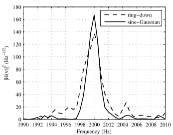
Figure 2: The normalised power spectral densities of the ring-down (dashed line) and sine-Gaussian (solid line) injections.

To demonstrate the operation of the algorithm, we inject a ring-down signal into $100$ s of Gaussian white noise with amplitude spectral density $10^{-22}$ Hz^-1/2. To investigate the response to a typical instrumental glitch which closely resembles our target waveform, we also inject a sine-Gaussian signal of the form

$$h(t)=h_{0}\sin\left[\omega\left(t-t_{0}\right)\right]e^{-(t-t_{0})^{2}/\tau^{2}},$$ (22)

where, $h_{0}$ is the maximum amplitude of the signal, $\omega$ is the angular frequency and $\tau$ is the decay time. Table 1 shows the parameter values used to generate the injections and Fig. 2 shows the power spectral density of each signal, calculated from the noisy data and normalised so that the noise follows a central $\chi^{2}$ distribution. It is the job of the algorithm to detect and differentiate between these two signals, only producing a candidate detection when the ring-down is present. The prior ranges used for each parameter are shown in Table 2.

Injection	Parameter		Value
RDI	Injection time	$t_{0}$	$10$s
	Initial amplitude	$h_{0}$	$7.0\times 10^{-21}$
	Central frequency	$\nu_{0}$	2 000 Hz
	Decay time	$\tau$	0.21 s
	SNR	$\rho$	20.4
SGI	Injection time	$t_{0}$	$80$ s
	Initial amplitude	$h_{0}$	$3.72\times 10^{-21}$
	Central frequency	$\nu_{0}$	2 000 Hz
	Decay time	$\tau$	0.21 s
	SNR	$\rho$	20.4

Table 1: Injected signal parameter values.

Parameter	Lower Limit	Upper Limit
$h_{0}$	$0$	$100\times 10^{-22}$
$\nu_{0}$	$1\,500$ Hz	$3\,000$ Hz
$\tau$	$0.05$ s	$0.5$ s

Table 2: Parameter prior ranges. The prior distributions are taken as uniform over these ranges.

Fig. 3 shows the odds ratio in each spectrogram time bin. The ring-down injection at $t=10$ s is strongly detected. Notice, however, that the sine-Gaussian we have injected to mimic an unwanted instrumental glitch is also detected, albeit with an odds ratio lower than that for the ring-down injection. To address this issue, we make a straightforward extension to the odds ratio to consider multiple hypotheses.

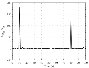
Figure 3: The log-odds in favour of a ring-down plus noise, versus the possibility that the power is due to noise alone. The first peak corresponds to the ring-down injection, the second to the sine-Gaussian injection.

III.3 Multiple hypothesis extension

To handle the possibility of sine-Gaussian instrumental glitches, we rewrite the posterior in the denominator as the sum of the probability of the noise model $M_{2}$ and a model for sine-Gaussian glitches, $M_{3}$. This gives

$$p(M_{-}|D,I)=p(M_{2}|D,I)+p(M_{3}|D,I)+\ldots\ ,$$ (23)

where $M_{-}$ denotes the proposition that the data does not contain a ring-down gravitational wave and the ellipsis is to emphasise the fact that this null-detection hypothesis $M_{-}$ may be further extended to include additional models for instrumental glitches. Similarly,

$$p(M_{+}|D,I)=p(M_{1}|D,I)+\ldots\ ,$$ (24)

where, again, it is straightforward to include additional signal models if desired. The result is that we are left with a comparison of the probability in favour of a gravitational wave with the probability of an instrumental glitch or that of the noise model, thus making maximal use of any knowledge we might have regarding transient features in the data.

Using $M_{-}$ now as the alternative hypothesis, we obtain a new odds ratio $O_{123}$:

$$O_{123}=\frac{p(M_{1}|D,I)}{p(M_{2}|D,I)+p(M_{3}|D,I)}.$$ (25)

Assuming the prior on each model is identical, the posterior probabilities in $O_{123}$ may be replaced by the evidences $p(D|M_{i},I)$ for $i=1,2,3$.

Fig. 4 shows the result of using this new expression for the odds ratio and the same data from the previous example. Since the parameterisation for the sine-Gaussian is identical to that of the ring-down, the priors in table 2 are also used to evaluate $p(M_{3}|D,I)$. There is no fundamental reason for using the same prior ranges for both models. Indeed, a realistic application would most likely have very different priors for the parameters in different models even if the parameterisation was the same. Here, the priors in Table 2 are used for both $M_{1}$ and $M_{3}$ for computational simplicity.

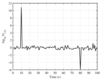
Figure 4: The log-odds in favour of a ring-down plus noise, versus the possibility that the power is due to noise alone or a sine-Gaussian glitch plus noise. The second (sine-Gaussian) peak seen in Fig. 3 is now seen as a dip.

The incorporation of the alternative model eliminates the previous problem of detecting sine-Gaussian signals with high odds ratios and, in fact, the odds ratio now strongly prefers the sine-Gaussian model to the ring-down model in the presence of the sine-Gaussian. Also note that the size of the peak indicating the ring-down has diminished quite substantially but is still clearly visible above the background. This reduction is due to a non-zero contribution from $p(M_{3}|D,I)$ in the denominator of $O_{123}$. Unless they are mutually exclusive in some way, the inclusion of additional models in the denominator of the odds ratio will generally increase the robustness of the search, at the cost of sensitivity.

IV Performance

We now investigate the performance of the algorithm by considering both formulations of the odds ratio, comparing the relative merits of each.

A ‘false alarm’ is defined as any unwanted transient event which causes the odds ratio to cross the threshold and generate a candidate detection. For white noise, false alarms are caused by spikes in the noise amplitude. The false alarm probability is calculated from the fraction of time bins in a large sample for which the odds ratio crosses the threshold when there is no ring-down signal present.

We investigate the response to ‘off-source’ data (i.e., white noise with no injections) by combining the results of ten 500 s spectrograms with a 1 s time resolution to give 5 000 off-source time bins. To evaluate the sensitivity of the search, ring-down signals of a constant signal-to-noise ratio are injected every other second into 500 second segments of white noise, synthesised in Matlab. This is then used to construct a 500 s spectrogram with 1 s time-resolution and 0.5 Hz frequency resolution for each set of injections, leading to 250 signal injections for each value of the signal-to-noise ratio. The fact that there are spectrogram time bins with no signal injection helps to prevent contamination from adjacent bins. We vary the signal-to-noise ratio through the value of $h_{0}$ only and always compare signals of equal bandwidth and at the same frequency, with the frequency held constant at $2$ kHz and the decay time at $207.5$ ms. The noise amplitude spectral density is $10^{-22}$ Hz^-1/2, representative of the LIGO noise floor at these frequencies.

When we make use of the glitch catalogue in the expanded odds ratio $O_{123}$ the objective is to be robust against unwanted glitches as well as spurious noise effects. Therefore, we also define a false alarm probability due to sine-Gaussians. This is found in exactly the same way as the sensitivity to ring-downs but using sine-Gaussian injections. The false alarm probability due to sine-Gaussians, therefore, is simply the fraction of the 250 injected sine-Gaussians which cause the odds ratio to exceed the threshold.

IV.1 $\textbf{O}_{\textrm{\scriptsize{12}}}$: ring-down vs noise

We take our desired false alarm probability here to be $1\%$. Fig. 5 shows the false alarm probability as a function of the log odds ratio threshold, $\log_{10}O_{\textrm{\scriptsize{thresh}}}$, and we see that a false alarm probability of $1\%$ is given by $\log_{10}O_{\textrm{\scriptsize{thresh}}}=4$.

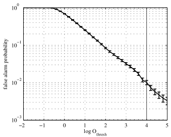
Figure 5: The false alarm probabilities in Gaussian white noise for different $\log_{10}O_{12}$ thresholds. Error bars represent $1\sigma$ Poissonian standard errors. The solid vertical line marks the threshold applied when using $\log_{10}O_{12}$.

Fig. 6 shows receiver operating characteristic (ROC) curves for $O_{12}$. ROC curves are plots of sensitivity (the probability of detecting what we are looking for) as a function of false alarm probability (the probability of claiming a detection due to a spurious noise event or instrumental glitch) for a given strength signal. The different false alarm probabilities correspond to different values of the detection threshold, $O_{\textrm{\scriptsize{thresh}}}$, and are found by reading the appropriate values from Fig. 5. When there are no injected signals, the only events to cause the odds ratio to cross the threshold are false alarms and the false alarm probability should be equal to the detection probability.

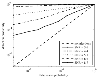
Figure 6: Receiver operating characteristic curves for $O_{12}$. False alarm probabilities are those from amplitude fluctuations in Gaussian white noise.

Although the ROC curves give some indication of how the sensitivity varies with injected signal strength, it is also helpful to examine efficiency curves, where the fraction of detected ring-downs is plotted against the injected signal strength, for a given threshold. Fig. 7 shows the detection efficiency using $\log_{10}O_{\textrm{\scriptsize{thresh}}}=4$ with corresponding false alarm probability of $1\%$.

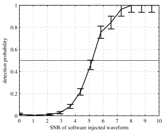
Figure 7: The detection efficiency obtained for $\log_{10}O_{12}$ using a threshold $\log_{10}O_{\textrm{\scriptsize thresh}}=4$. Error bars show $1\sigma$ standard Possonian errors.

The algorithm’s performance is best summarised by the signal-to-noise ratio required to give a detection probability of $50\%$ while maintaining the desired false alarm probability. A signal-to-noise ratio $\rho=5.2$ is required for $50\%$ ring-down detection, corresponding to an initial ring-down amplitude at Earth of $h_{0}=1.8\times 10^{-21}$ at current LIGO sensitivities.

Equation 3 on page 3 relates $h_{0}$ to the distance to the source and the energy emitted as gravitational waves. Using this equation and assuming the fiducial distance of $15$ kpc, the energy required to generate this initial ring-down amplitude at the Earth is $1.3\times 10^{-5}M_{\astrosun}c^{2}$. Conversely, when we assume the fiducial energy in gravitational waves of $10^{-11}M_{\astrosun}$, the distance to the source must be $13.2$ pc for this amplitude. These results are summarised in Table 3.

IV.2 $\textbf{O}_{\textrm{\scriptsize{123}}}$: Ring-down vs noise or sine-Gaussian glitch

We now evaluate the performance of the algorithm using the more robust comparison between ring-downs, white noise and sine-Gaussians.

The response of $O_{123}$ to sine-Gaussians is compared with the response to ring-down injections in Fig. 8. The horizontal axis shows the signal-to-noise ratio of each type of injected signal (ring-down or sine-Gaussian) and the vertical axis gives the mean value of $\log_{10}O_{123}$, calculated from 250 injections of each signal type. The response can be separated into three regions of signal-to-noise ratio, $\rho$:

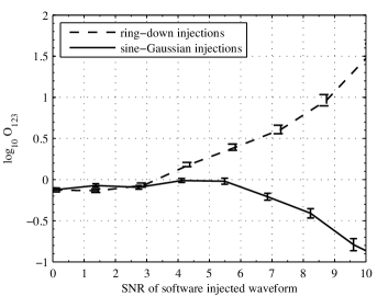
Figure 8: The mean value of $\log_{10}O_{123}$ for varying strengths of signal-to-noise ratio. Results of ring-down injections are shown by the dashed curve, while the solid curve shows the results of the sine-Gaussian injections. Error bars represent $1\sigma$ standard errors in the mean values of $\log_{10}O_{123}$.

$\rho\lesssim 3$

: there is no response to sine-Gaussians or ring-downs and any signal present is indistinguishable from noise.

$3\lesssim\rho\lesssim 5$

: the algorithm begins to respond to the ring-down injections. The sine-Gaussian injections generate a very slight rise in the log odds.

$\rho\gtrsim 5$

: the odds in favour of a ring-down begin to grow for the ring-down injections and rapidly falls off for the sine-Gaussian injections.

We use the intermediate region (i.e., where $3\lesssim\rho\lesssim 5$) to assume a worst-case scenario where all sine-Gaussian glitches have a signal-to-noise ratio $\rho\sim 4$ and compute the false alarm probability from sine-Gaussians for different odds ratio thresholds. The results are shown in Fig. 9.

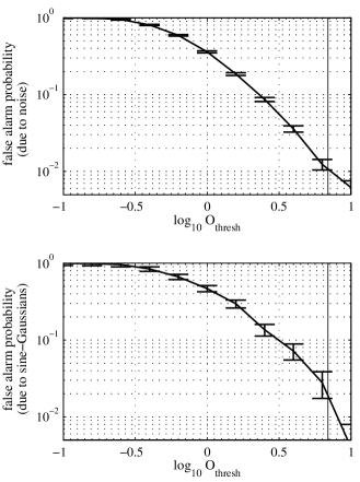
Figure 9: Top panel: false alarm probabilities and corresponding $\log_{10}O_{123}$ thresholds for Gaussian white noise. Bottom panel: false alarm probabilities and corresponding $\log_{10}O_{123}$ thresholds for sine-Gaussians with signal-to-noise ratio $\rho\sim 4$. In each case, the solid vertical line indicates the threshold required for a $1\%$ false alarm probability in Gaussian white noise. Error bars show $1\sigma$ Poissonian standard errors.

We now find that the threshold required to give a false alarm probability of $1\%$ in Gaussian white noise is $\log_{10}O_{\textrm{\scriptsize{thresh}}}=0.84$. This corresponds to a false alarm probability of $10\%$ when the data contains a sine-Gaussian. We note two points here:

• we have assumed the presence of sine-Gaussian glitches a priori. While it is appropriate to assume the presence of Gaussian white noise, we do not have a population model for the sine-Gaussian glitches. A more informative estimate of the probability of mistakenly detecting a sine-Gaussian glitch should fold in the effects of such a population model through the prior on $M_{3}$. In this work, we are more interested in demonstrating the inherent ability of the algorithm to discriminate between similar waveforms and this will not be considered.

• Only sine-Gaussians with signal-to-noise ratios of $\rho\sim 4$ are considered. Away from this value, the odds ratio drops off rapidly so that the $10\%$ false alarm probability can be regarded as an upper limit for sine-Gaussian glitches.

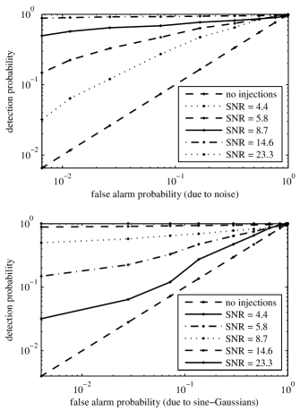
Figure 10: Receiver operating characteristic curves for $O_{123}$. Top panel: ROC curve with false alarm probabilities due to spurious noise events. Bottom panel: ROC curve with false alarm probabilities due to sine-Gaussian glitches.

Because we have two possible sources of false alarms, sine-Gaussians and noise events, we produce ROC figures for each, shown in each of the panels of Fig. 10.

For comparison with the sensitivity of $O_{12}$ Fig. 11 shows the detection efficiency for $O_{123}$. We find that the signal-to-noise ratio required for $50\%$ detection efficiency and $1\%$ false alarm probability in Gaussian white noise is $\rho^{50\%}=8.0$.

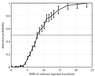
Figure 11: The detection efficiency obtained for $\log_{10}O_{123}$ using a threshold $\log_{10}O_{\textrm{\scriptsize thresh}}=0.84$. The solid horizontal line indicates $50\%$ detection efficiency. Error bars show $1\sigma$ Poissonian standard errors.

Again, it is important to consider these results in an astrophysical context. With the noise amplitude spectral density used for these investigations ($10^{-22}$ Hz^-1/2), a ring-down signal-to-noise ratio $\rho=8.0$ corresponds to an initial amplitude $h_{0}=2.9\times 10^{-21}$ Hz^-1/2. The gravitational wave energy required to produce a ring-down signal with $50\%$ detection probability at the Earth with this amplitude is $3.3\times 10^{-5}M_{\astrosun}c^{2}$ for a source at $15$ kpc. Similarly, if we assume that $10^{-11}M_{\astrosun}c^{2}$ is emitted as gravitational waves , the source must lie at $8.2$ pc. These results are summarised and compared with those from $O_{12}$ in Table 3.

Parameter	Symbol	Value Using $O_{12}$	Value Using $O_{123}$
Log odds threshold	$\log_{10}O_{\textrm{\scriptsize{thresh}}}$	$4$	$0.84$
False alarm probability (due to noise)	$p(-|N)$	$1\%$	$1\%$
False alarm probability (due to sine-Gaussians)	$p(-|SG)$	$-$	$10\%$
Signal-to-noise	$\rho^{50\%}$	$5.2$	$8.0$
Initial strain amplitude	$h_{0}^{50\%}$	$1.8\times 10^{-21}$	$2.9\times 10^{-21}$
GW Energy	$E_{\textrm{\scriptsize{GW}}}^{50\%}$	$1.3\times 10^{-5}M_{\astrosun}c^{2}$	$3.3\times 10^{-5}M_{\astrosun}c^{2}$
Range	$D_{\textrm{\scriptsize{GW}}}^{50\%}$	$13.2$ pc	$8.2$ pc
Root-sum-squared strain	$h_{rss}^{50\%}$	$4.1\times 10^{-22}$	$6.6\times 10^{-22}$

Table 3: Simulated sensitivity estimates for $50\%$ detection efficiency and corresponding false alarm probabilities. $p(-|N)$ is the probability of a false alarm from white noise for the given threshold $\log_{10}O_{\textrm{\scriptsize{thresh}}}$. Similarly, $p(-|SG)$ is the probability of a false alarm given a sine-Gaussian event. All estimates assume a ring-down frequency $\nu=2$ kHz, decay timescale $\tau=207.5$ ms and a noise amplitude spectral density $10^{-22}$ Hz^-1/2. $E_{\textrm{\scriptsize{GW}}}^{50\%}$ is calculated for a distance $D=15$ kpc and $D_{\textrm{\scriptsize{GW}}}^{50\%}$ is calculated for an energy in gravitational waves of $10^{-11}M_{\astrosun}c^{2}$.

IV.3 Comparison to matched filtering

The LIGO Algorithm Library (LAL) LAL and LALapps software repositories used for much of the gravitational wave data analysis within the LIGO Scientific Collabora- tion (LSC) contain software for performing a matched filter based search for ring-down signals. Currently this is being used to search for ring-downs from perturbed black holes Goggin and the LIGO Scientific Collaboration (2006). The software can be used to compare the false alarm probability of the matched filtering method with our method by running it on simulated white noise for the range of parameters given in Table 2 . The template bank for the matched filtering was produced to give a maximum mismatch between adjacent templates of $1\%$.

We define the false alarm probability to be the fraction of detection candidates generated by the algorithm whose signal-to-noise ratio crosses a given threshold. Fig. 12 shows the false alarm probability as a function of signal- to-noise ratio threshold: for a false alarm probabilty of $1\%$, we require a signal-to-noise ratio threshold of $5.85$ (compared with $\rho=5.2$ for the evidence based search).

It may seem surprising that the evidence-based search marginally out-performs matched filtering. It is important to remember, however, that the approaches are by no means equivalent: matched filtering searches for consistency with a given waveform, whereas the evidence-based approach searches for both consistency with the same waveform but also for inconsistency with a noise model. Since the noise model is highly sensitive to excess power (which exponentially decreases its likelihood), it does not seem unreasonable that there is a slight disparity between the approaches.

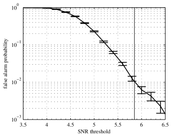
Figure 12: The cumulative percentage of triggers produced by a matched filter based ring-down signal search code over a range of signal-to-noise ratios for data consisting of simulated Gaussian white noise. Error bars indicate 1$\sigma$ Poissonian standard errors. The solid vertical line indicates the $\rho=5.85$ threshold for a $1\%$ false alarm probability.

V Further extensions

We now highlight some outstanding issues and possible important extensions to this work which may be required to make the transition from ‘proof-of-concept’ to a useful search tool. Particularly, we address the issues of constructing the catalogue of alternative hypotheses, the extension to a multi-detector analysis and the outline for a full analysis pipeline.

Glitch classification

It is likely that the inclusion of extra information regarding glitches will increase robustness against instrumental transients which would otherwise generate a candidate detection event. For this to be effective, we require some classification scheme for these instrumental glitches which would allow the construction of a catalogue of glitch models as well as their associated priors.

Essentially, what is required is an automated pattern recognition tool which could be ‘trained’ on off-source interferometer data and used to generate a generic library of transient features. Fortunately, on-going detector characterisation work aims to perform such an analysis Mukherjee (2006) (on behalf of the LIGO Science Collaboration).

Multiple detector case

A potential issue with this search is in fact the prevalence of instrumental ring-downs already present in the interferometer data. Unless such features can be vetoed using known instrumental couplings, for example Ajith et al. (2006), the only way to distinguish these from the targeted gravitational wave ring-down is to search for coincidences between multiple detectors.

Here, we benefit again from the simplicity of the Bayesian formalism. In the single detector case outlined in this work, we aim to compute the posterior probability for some gravitational wave model, given the interferometer data and some background information. In the multi-detector case we still seek the posterior probability for some model but now using the information contained in each detector’s output. Suppose then that we have some gravitational wave model $M_{\textrm{\scriptsize{GW}}}$ and detector outputs $D_{1}$ and $D_{2}$. We can immediately write down the posterior for $M_{\textrm{\scriptsize{GW}}}$ using Bayes’ theorem

$$p(M_{\textrm{\scriptsize{GW}}}|D_{1},D_{2},I)=\frac{p(M_{\textrm{\scriptsize{GW}}}|I)p(D_{1},D_{2}|M_{\textrm{\scriptsize{GW}}},I)}{p(D_{1},D_{2}|I)},$$ (26)

where the gravitational wave model $M_{\textrm{\scriptsize{GW}}}$ factors in the appropriate detector response functions for the source sky position and for detectors with uncorrelated output, the joint probabilities are the products of the individual probabilities. For $N$ detectors

$$p(M_{\textrm{\scriptsize{GW}}}|\{D\},I)=p(M_{\textrm{\scriptsize{GW}}}|I)\prod_{i=1}^{N}\frac{p(D_{i}|M_{\textrm{\scriptsize{GW}}},I)}{p(D_{i}|I)}$$ (27)

and we can again eliminate the denominator by comparing the relative probabilities of different models via the odds ratio. Notice, however, that if the probability from one detector is very large but low in the other detectors it is still possible to get a high posterior across all the detectors. It would, therefore, be sensible to apply a cut to the data such that the odds must cross some threshold for each individual detector before considering the multi-detector case.

Analysis pipeline

Finally, we present the outline for a planned analysis pipeline in Fig. 13. Here, we assume a network of two detectors and that there is no correlation in the output from each.

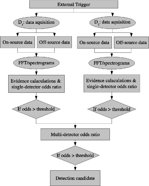
Figure 13: Planned multi-detector, evidence-based analysis pipeline.

Upon reception of an external trigger, such as a pulsar glitch or soft $\gamma$-ray repeater flare, we would retrieve interferometer data from near the event (on-source data). The length of data required will typically depend on the time resolution of the external trigger. Additionally, we require data preceding the external trigger to provide some estimate of the background odds ratio and hence set the threshold for the desired false alarm probability.

Following the acquisition of both on and off-source data for each detector, we transform to the Fourier domain and construct spectrograms of each. From here, the methods outlined in this work can be used to compute the evidences for each gravitational wave and glitch model and the odds ratio can be computed for each detector using on and off-source data.

If the odds in both detectors cross some appropriate threshold, then we can go on to calculate the multi-detector odds ratio. If this multi-detector odds ratio also crosses a threshold set from off-source data then we have a candidate detection.

Alternatively, if the odds ratio from just one of the detectors in the network crosses the respective threshold, then there is probably good evidence for a glitch. Further examination of the odds ratios for each glitch model may reveal its nature and the information could conceivably be used to update the prior on that particular model in future studies.

VI Concluding remarks

We have examined the feasibility of using a Bayesian evidence discriminator in an externally-triggered search for gravitational waves produced by neutron star quasi-normal mode ring-downs. The evidence may be thought of as the total probability of the data given some model. By comparing the evidences for competing models via the ‘odds ratio’, we can naturally make maximal use of prior information regarding the source as well as any information available from detector characterisation studies.

This is particularly important in the single-detector case. Here there may be instrumental transients or ‘glitches’ which would otherwise generate a detection candidate in algorithms which only look for consistency with the target model. We begin with a simple formulation of the odds ratio, $O_{12}$, where we compare the probability of a noisy ring-down model with the probability of noise alone. We find this yields a $50\%$ detection efficiency for ring-downs with frequency $2$ kHz, decay time $0.21$ s and signal-to-noise ratio $\rho=5.2$ for a $1\%$ false alarm probability in Gaussian white noise of amplitude spectral density $10^{-22}$ Hz^-1/2. To obtain the same false alarm probability using matched filtering we require a signal-to-noise ratio threshold $\rho=5.85$. As described in section IV.3 this disparity is most likely due to the fundamental difference between using the odds ratio, which compares the evidences from two or more competing models and matched filtering, which only searches for consistency with a single target waveform.

Assuming $10^{-11}M_{\astrosun}c^{2}$ is emitted as gravitational waves, these sources are observable to a distance of $13.2$ pc. Conversely, a source at a distance of $15$ kpc requires an energy of $1.3\times 10^{-5}M_{\astrosun}c^{2}$ to be emitted as gravitational waves. This is several orders of magnitude greater than the typical energy we might expect from a pulsar glitch, making these sources a more attractive target for next-generation detectors such as advanced LIGO Fritschel (2003) and GEO-HF Willke et al. (2006). If, for example, we consider advanced LIGO with a factor $\sim 10$ improvement in sensitivity over LIGO, the energy required to produce the same signal-to-noise ratio drops to $\sim 1.0\times 10^{-7}M_{\astrosun}c^{2}$. While this is still well below our fiducial pulsar glitch gravitational wave energy of $10^{-11}M_{\astrosun}c^{2}$, it is comparable to the gravitational wave energy expected to be emitted following the axisymmetric collapse of the core of a massive star, some fraction of which will be channelled into the oscillatory modes of the proto-neutron star Ferrari et al. (2003); Dimmelmeier et al. (2002). Again, if we assume the fiducial gravitational wave energy of $10^{-11}M_{\astrosun}c^{2}$, advanced LIGO will be sensitive to neutron star ring-downs at a distance of $148$ pc.

We find the simple comparison between white noise and ring-downs is insufficient to discriminate between different types of signal and will be fooled by any transient departure from Gaussianity in the noise. Robustness is improved by including a toy catalogue of glitch models (a sine-Gaussian). The odds ratio may then be extended (i.e., $O_{123}$) to mitigate the effects of these unwanted signals at a relatively small sensitivity cost: a ring-down signal-to-noise ratio of $\rho=8.0$ is now required for the $50\%$ ring-down detection efficiency and $1\%$ false alarm probability due to Gaussian white noise, so that the total gravitational wave energy required for $50\%$ detection probability of a source at $15$ kpc is now $3.3\times 10^{-5}M_{\astrosun}c^{2}$ and the observable range is now $8.2$ pc. With advanced LIGO sensitivity, these estimates improve to $2.7\times 10^{-8}M_{\astrosun}c^{2}$ and $91.6$ pc for the energy in gravitational waves and the observable range, respectively. We also find that this extened odds ratio only has a $10\%$ chance of falsely identifying a sine-Gaussian as a ring-down. This assumes a worst-case scenario in which the sine-Gaussian has a signal-to-noise ratio $\rho\sim 4$ (where the algorithm’s response to these signals peaks). This is therefore an upper limit so that the false alarm rate from sine-Gaussians will generally be much lower.

Finally, we have made mention of some of the future work required to use the methodology in this work in a search for gravitational waves. For the single detector case, it will be necessary to acquire an appropriate catalogue of glitch models and associated prior probabilities for their parameters. The extension to the multi-detector case will require considerable modification to the waveform model to account for light travel time between detectors and the appropriate antenna response functions for a given sky location. For this search, we are at an advantage in that we know the source location and event time, and hence the factors introduced by the antenna response and time delay are known. We note, however, that if this was not so, as would be the case for an all-sky search or where we had a trigger but no source location, it would be necessary to marginalise over the source location which would significantly complicate the evidence calculation.

With a clear idea of the future analysis pipeline, the next step is to characterise the algorithm response using real interferometer data and all the consequences of non-Gaussian noise.