Uniqueness of de Sitter Space

Abstract

All inextendible null geodesics in four dimensional de Sitter space $dS^{4}$ are complete and globally achronal. This achronality is related to the fact that all observer horizons in $dS^{4}$ are eternal, i.e. extend from future infinity ${\cal J}^{+}$ all the way back to past infinity ${\cal J}^{-}$. We show that the property of having a null line (inextendible achronal null geodesic) that extends from ${\cal J}^{-}$ to ${\cal J}^{+}$ characterizes $dS^{4}$ among all globally hyperbolic and asymptotically de Sitter spacetimes satisfying the vacuum Einstein equations with positive cosmological constant. This result is then further extended to allow for a class of matter models that includes perfect fluids.

1 Introduction

Asymptotically de Sitter spacetimes can be roughly thought of as solutions to the Einstein equations with positive cosmological constant having a spacelike boundary at infinity ${\cal J}$. These spacetimes naturally arise in a number of contexts, such as in the study of inflationary cosmological models. An asymptotically de Sitter spacetime is said to be asymptotically simple provided every null geodesic extends all the way from past infinity ${\cal J}^{-}$ to future infinity ${\cal J}^{+}$. Such spacetimes are, of course, modelled on de Sitter space $dS^{n}$ itself, which conformally embeds into the Einstein cylinder, acquiring there a past conformal infinity ${\cal J}^{-}$ and future conformal infinity ${\cal J}^{+}$, each spacelike and diffeomorphic to the $(n-1)$-sphere. An additional causal feature of de Sitter space is that every inextendible null geodesic in it is globally achronal, i.e., never enters into its own chronological future or past. Such null geodesics are referred to as null lines.

As it turns out, the occurrence of null lines is a very particular feature of de Sitter space. In [12] it is proved that this property characterizes $dS^{4}$ among all four dimensional asymptotically simple and de Sitter spacetimes:

Theorem 1.1

Let $(\tilde{M},\tilde{g})$ be an asymptotically simple and de Sitter spacetime of dimension $n=4$ that satisfies the vacuum Einstein equations with positive cosmological constant. If $\tilde{M}$ contains a null line, then $\tilde{M}$ is isometric to de Sitter space $dS^{4}$.

As discussed in [12, 13], this theorem can be interpreted in terms of the initial value problem in the following way: Friedrich’s work [10] on the nonlinear stability of de Sitter space shows that the set of asymptotically simple solutions to the Einstein equations with positive cosmological constant is open in the set of all maximal globally hyperbolic solutions with compact spatial sections. As a consequence, by slightly perturbing the initial data on a fixed Cauchy surface of $dS^{4}$ we get in general an asymptotically simple solution of the Einstein equations different from $dS^{4}$. Thus by virtue of theorem 1.1, such a spacetime has no null lines. In other words, a small generic perturbation of the initial data destroys all null lines. This suggests that the so-called generic condition of singularity theory [15] is in fact generic with respect to perturbations of the initial data.

Alternatively, we could say that no other asymptotically simple solution of the Einstein equations besides $dS^{4}$ develops eternal observer horizons. By definition, an observer horizon ${\cal A}$ is the past achronal boundary $\partial I^{-}(\gamma)$ of a future inextendible timelike curve $\gamma$, thus ${\cal A}$ is ruled by future inextendible achronal null geodesics. As follows from previous comments, in the case of de Sitter space, observer horizons are eternal, that is, all null generators of ${\cal A}$ extend from ${\cal J}^{+}$ all the way back to ${\cal J}^{-}$.

Since the observer horizon is the boundary of the region of spacetime that can be observed by $\gamma$, the question arises as to whether at one point $\gamma$ would be able to observe the whole of space. More precisely, we want to know if there exists $q\in\tilde{M}$ such that $I^{-}(q)$ would contain a Cauchy surface of spacetime. Gao and Wald were able to answer this question affirmatively for globally hyperbolic spacetimes with compact Cauchy surfaces, assuming null geodesic completeness, the null energy condition and the null generic condition [14]. Thus, as expressed by Bousso [5], asymptotically de Sitter spacetimes satisfying the conditions of the Gao and Wald result, have Penrose diagrams that are “tall” compared to de Sitter space.

Though no set of the form $I^{-}(q)$ in $dS^{4}$ contains a Cauchy surface, $I^{-}(q)$ gets arbitrarily close to doing so as $q\to{\cal J}^{+}$. However, notice that de Sitter space is not a counterexample to Gao and Wald’s result, since $dS^{4}$ does not satisfy the null generic condition. Actually, the latter remark enables us to interpret theorem 1.1 as a rigid version of the Gao and Wald result in the asymptotically simple (and vacuum) context: by dropping the null generic hypothesis in [14] the conclusion will only fail if $(\tilde{M},\tilde{g})$ is isometric to $dS^{4}$.

The aim of the present paper is to show that two of the basic assumptions in Theorem 1.1 can be substantially weakened. Firstly, asymptotic simplicity is a stringent global condition that rules out from the onset the possible presence of singularities and black holes; examples such as Schwarzschild de Sitter spacetime never enter the discussion. In section 3 we show that, provided there is a null line that extends from ${\cal J}^{-}$ to ${\cal J}^{+}$, the assumption of asymptotic simplicity can be replaced by the much milder assumption of global hyperbolicity, thus allowing a priori the occurrence of singularities and black holes.

In precise terms, we show

Theorem 1.2

Let $(\tilde{M},\tilde{g})$ be a globally hyperbolic and asymptotically de Sitter spacetime of dimension $n=4$ satisfying the vacuum Einstein equations with positive cosmological constant. If $\tilde{M}$ has a null line with endpoints $p\in{\cal J}^{-}$, $q\in{\cal J}^{+}$ then $(\tilde{M},\tilde{g})$ is isometric to an open subset of de Sitter space containing a Cauchy surface.

In fact, as is discussed in more detail in section 3, if $(\tilde{M},\tilde{g})$ is the maximal development of initial data from one of its Cauchy surfaces then it must be globally isometric to de Sitter space.

Secondly, we have long felt that the vacuum assumption in theorem 1.2 should not be essential, that the conclusion should still hold even if matter is allowed a priori to be present. In section 4 we establish a version of theorem 1.2 for spacetimes satisfying the Einstein equations (with $\Lambda>0$) with respect to a class of matter models that contains perfect fluids; see theorem 4.1.

In the next section we set notation, give some precise definitions and establish some preliminary results.

2 Preliminaries

Throughout this paper we will be using standard notation for causal sets and relations. Refer to [21, 19] for the main results and definitions in causal theory.

2.1 Definitions and the null splitting theorem

As usual, a spacetime $(\tilde{M},\tilde{g})$ is a connected, time-oriented four dimensional Lorentzian manifold. Following Penrose, we say that a spacetime $(\tilde{M},\tilde{g})$ admits a conformal boundary ${\cal J}$ if there exists a spacetime with non-empty boundary $(M,g)$ such that

1. $\tilde{M}$ is the interior of $M$ and ${\cal J}=\partial M$, thus $M=\tilde{M}\cup{\cal J}$.

2. There exists $\Omega\in{\cal C}^{\infty}({M})$ such that

   1. ${g}=\Omega^{2}\tilde{g}$ on $\tilde{M}$,

   2. $\Omega>0$ on $\tilde{M}$,

   3. $\Omega=0$ and $d\Omega\neq 0$ on ${\cal J}$.

In this setting $g$ is referred to as the unphysical metric, ${\cal J}$ is called the conformal boundary of $\tilde{M}$ in $M$ and $\Omega$ its defining function.

Further, we will say a spacetime $(\tilde{M},\tilde{g})$ admitting a conformal boundary ${\cal J}$ is asymptotically de Sitter if ${\cal J}$ is spacelike. Thus, by considering the standard conformal embedding of $dS^{n}$ in the Einstein cylinder we clearly note that $dS^{n}$ is an asymptotically de Sitter space itself. However, we emphasize that the definition of asymptotically de Sitter does not require ${\cal J}$ to be compact. This lack of compactness causes some complications in some of the arguments.

Many physically relevant scenarios in General Relativity are modelled by asymptotically de Sitter spacetimes. Schwarzchild de Sitter spacetime, which models a black hole sitting in a positively curved background, is one such example (with a noncompact ${\cal J}$, in fact). Other examples can be found in the context of cosmology, for instance the dust-filled Friedmann-Robertson-Walker models which satisfy the Eintein equations with $\Lambda>0$.

Because of the spacelike character of ${\cal J}$, in an asymptotically de Sitter spacetime, ${\cal J}$ can be decomposed as the union of the disjoint sets ${\cal J}^{+}=\{p\in{\cal J}\mid\nabla\Omega_{p}\ \textrm{is future pointing}\}$ and ${\cal J}^{-}=\{p\in{\cal J}\mid\nabla\Omega_{p}\ \textrm{is past pointing}\}$. As a consequence, ${\cal J}^{+}\subset I^{+}(\tilde{M},M)$ and ${\cal J}^{-}\subset I^{-}(\tilde{M},M)$. It follows as well that both sets ${\cal J}^{+}$, ${\cal J}^{-}$ are acausal in $M$.

An asymptotically de Sitter spacetime is said to be asymptotically simple if every inextendible null geodesic has endpoints on ${\cal J}$. Such spacetimes are, in particular, null geodesically complete. A null line is a globally achronal inextendible null geodesic. Recall that a spacetime satisfying the Einstein equations is said to obey the null energy condition if $T(K,K)\geq 0$ for all null vectors $K\in TM$. As theorem 1.1 shows, the occurrence of a null line and the null energy condition are incompatible for asymptotically simple and de Sitter solutions to vacuum Einstein equations different from $dS^{4}$.

Theorem 1.1 is a consequence of the null splitting theorem [11], which plays an important role in the proof of theorem 1.2 as well. Here is the precise statement:

Theorem 2.1

Let $(M,g)$ be a null geodesically complete spacetime which obeys the null energy condition. If $M$ admits a null line $\eta$, then $\eta$ is contained in a smooth properly embedded, achronal and totally geodesic null hypersurface $S$.

Remark 2.2

The proof of the null splitting theorem actually shows how to construct such an $S$: let $\partial_{0}I^{\pm}(\eta)$ be the connected components of $\partial I^{\pm}(\eta)$ containing $\eta$, then $\partial_{0}I^{+}(\eta)$ and $\partial_{0}I^{-}(\eta)$ agree and this common surface satisfies all aforementioned properties. Moreover, the proof also shows that future null completeness of $\partial_{0}I^{-}(\eta)$ and past null completeness of $\partial_{0}I^{+}(\eta)$ are sufficient for the result to hold (see remark IV.2 in [11].) This point is essential to the proof of Theorem 1.2.

2.2 Extension lemmas

In order to prove theorem 1.2 we are faced with the technical difficulty of dealing with a spacetime with boundary. Thus it is convenient to think of our spacetime with boundary as embedded in a larger open spacetime. This can always be done, as the next result shows.

Lemma 2.3

Every spacetime with boundary $(M,g)$ admits an extension to a spacetime $(N,h)$.

Proof: First extend $M$ to a smooth manifold $M^{\prime}$ by means of attaching collars to all the components of $\partial M$. Since $M$ is time orientable, there exists a timelike vector field $V\in{\cal X}(M)$. Let us extend $V$ to all of $M^{\prime}$ and let $W=\{p\in M^{\prime}\mid V_{p}\neq 0\}$. Clearly $W$ is an open subset of $M^{\prime}$ containing all of $M$, so without loss of generality we can assume $M^{\prime}=W$.

Let $p\in\partial M$ and choose a $M^{\prime}$-chart ${\cal U}_{p}$ around it. Now let $g=g_{ij}dx^{i}dx^{j}$ be the coordinate expression of $g$ in the $M$-chart $M\cap{\cal U}_{p}$. Since the $g_{ij}$’s are smooth functions on $M\cap{\cal U}_{p}$, they can be smoothly extended to an $M^{\prime}$-neighborhood ${\cal U}^{\prime}_{p}\subset{\cal U}_{p}$ with $M\cap{\cal U}^{\prime}_{p}=M\cap{\cal U}_{p}$. Let us denote by $g^{\prime}_{ij}$ such extensions. It is important to notice that ${\cal U}^{\prime}_{p}$ can be chosen in such a way that $g^{\prime}=g^{\prime}_{ij}{dy}^{i}{dy}^{j}$ is a Lorentz metric on ${\cal U}^{\prime}_{p}$ with $g^{\prime}(V,V)<0$. Choose a cover $\{{\cal U}_{\alpha}\}$ of $\partial M$ by such open sets and let us define $h_{\alpha}=2e_{0}^{*}\otimes e_{0}^{*}+g^{\prime}_{\alpha}$ on $\{{\cal U}_{\alpha}\}$, where $e_{0}$ denotes the unit vector field (with respect to $g^{\prime}$) in the direction of $V$. Further consider a smooth partition of unity $f_{\alpha}$ subordinated to $\{{\cal U}_{\alpha}\}$, thus $h_{0}=\sum_{\alpha}f_{\alpha}h_{\alpha}$ is a Riemannian metric on ${\cal U}=\cup_{\alpha}{\cal U}_{\alpha}$.

Finally, let $X$ be the unit vector field (with respect to $h_{0}$) in the direction of $V$, let $\omega$ be the covector $h_{0}$-related to $X$ and let $g^{\prime\prime}=h_{0}-2\omega\otimes\omega$. It is straightforward to check that $g^{\prime\prime}$ is a Lorentz metric on ${\cal U}$ that agrees with $g$ on the overlap ${\cal U}\cap M$. Thus by gluing $g^{\prime\prime}$ and $g$ together we obtain a Lorentz metric $h$ on $N={\cal U}\cup M$. Notice $h$ is smooth since ${\cal U}$ is open. $\Box$

Now that we have successfully extended our spacetime with boundary, we would like to verify that our extension inherits some important causal properties. More precisely, we show that global hyperbolicity extends “beyond ${\cal J}$” in the asymptotically de Sitter setting. That is, if $(\tilde{M},\tilde{g})$ is globally hyperbolic, then we can choose a globally hyperbolic extension $(N,h)$ of it.

Lemma 2.4

Let $(\tilde{M},\tilde{g})$ be a globally hyperbolic and asymptotically de Sitter spacetime, then $(\tilde{M},\tilde{g})$ can be embedded in a globally hyperbolic spacetime $(N,h)$ such that ${\cal J}$ topologically separates $\tilde{M}$ and $N-\tilde{M}$.

Proof: It suffices to show $(\tilde{M},\tilde{g})$ can be extended past ${\cal J}^{-}$ since a similar procedure can be used to extend $(\tilde{M},\tilde{g})$ beyond ${\cal J}^{+}$, thus without loss of generality we can assume ${\cal J}={\cal J}^{-}$. By lemma 2.3 there is an open spacetime $(N_{0},h)$ extending $(M,g)$. Since $N_{0}$ is obtained from $M$ by attaching collars, the separation part of the proposition holds. As a consequence ${\cal J}$ is acausal in $N_{0}$, hence the Cauchy development $D({\cal J},N_{0})$ is an open subset of $N_{0}$. Thus $N=M\cup D({\cal J},N_{0})$ is an open spacetime containing $M$. We claim that $(N,h)$ is globally hyperbolic. In fact, it is easy to see that if $S$ is a Cauchy surface for $(\tilde{M},\tilde{g})$ then it is also a Cauchy surface for $(N,h)$. Indeed, any inextendible causal curve in $N$ must meet $M$, and hence will intersect $S$. $\Box$

3 Rigidity without asymptotic simplicity

The main aim of this section is to prove the following theorem and discuss some of its consequences:

Theorem 3.1

Let $(\tilde{M},\tilde{g})$ be a globally hyperbolic and asymptotically de Sitter spacetime of dimension $n=4$ satisfying the vacuum Einstein equations with positive cosmological constant. If $\tilde{M}$ has a null line with endpoints $p\in{\cal J}^{-}$, $q\in{\cal J}^{+}$ then $(\tilde{M},\tilde{g})$ is isometric to an open subset of de Sitter space containing a Cauchy surface.

Before moving into the proof, we would like to comment that the result is sharp, in the sense that there exists globally hyperbolic proper subsets of $dS^{4}$ which contain a null line with endpoints in ${\cal J}$ (see fig. 1 above); see however theorem 3.7. We remark also that some globally hyperbolic and asymptotically de Sitter spacetimes, such as Schwarzschild de Sitter space, do possess null lines although they do not extend to ${\cal J}$.

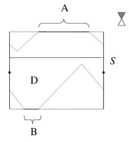
Figure 1: $D=I^{+}(B)\cap I^{-}(A)$ is an asymptotically de Sitter and globally hyperbolic open subset of de Sitter space with Cauchy surface $S$.

We begin the proof of theorem 3.1 by considering a couple of technical lemmas, which establish that the achronal boundaries $\partial I^{+}(\eta)$, $\partial I^{-}(\eta)$ are the result of exponentiating the respective null cones about the endpoints of $\eta$ in ${\cal J}$.

Lemma 3.2

Let $(\tilde{M},\tilde{g})$ be a globally hyperbolic and asymptotically de Sitter spacetime and $\eta$ a future directed causal curve in $M$. Further assume $p\in{\cal J}^{-}$ is the past endpoint of $\eta$. Then

1. ${\partial I^{+}(\eta)=J^{+}(p,N)-(I^{+}(p,N)\cup\{p\})}$,

2. $J^{+}(N_{p},N)\cap\tilde{M}\subset D^{+}(N_{p},N)\cap\tilde{M}$,

where $N_{p}:=\partial_{N}I^{+}(p,N)$ and $N$ is a globally hyperbolic extension of $(M,g)$.

Proof: First notice that by global hyperbolicity the set $J^{+}(p,N)$ is closed in $N$, and as a consequence

$$\partial_{N}I^{+}(p,N)=J^{+}(p,N)-I^{+}(p,N).$$ (3.1)

Thus by the acausality of ${\cal J}^{-}$ we have

$$\tilde{M}\cap\partial_{N}I^{+}(p,N)=\partial_{N}I^{+}(p,N)-\{p\}$$ (3.2)

Let us show now $I^{+}(\eta)=I^{+}(p,N)$. It is clear that $I^{+}(\eta)\subset I^{+}(p,N)$. Conversely, let $x\in I^{+}(p,N)$ and let us take $y\in\eta\cap I^{-}(x,N)$. Since any future timelike curve from $y$ to $x$ has to be contained in $\tilde{M}$ due to the separating properties of ${\cal J}^{-}$, we have $x\in I^{+}(\eta)$ and thus $I^{+}(p,N)\subset I^{+}(\eta)$ is proven. As a consequence $\partial I^{+}(\eta)=\partial_{\tilde{M}}I^{+}(p,N)$. Finally, since $I^{+}(p,N)$ is an open set in $N$ we get

$$\partial_{\tilde{M}}I^{+}(p,N)=\tilde{M}\cap\partial_{N}I^{+}(p,N).$$ (3.3)

Then the first assertion follows.

To prove the second part of the lemma we proceed by contradiction. Thus let us assume $x\in J^{+}(N_{p},N)\cap\tilde{M}-D^{+}(N_{p},N)\cap\tilde{M}$, hence it follows $x\in I^{+}(p,N)$. On the other hand, since $x\notin D^{+}(N_{p},N)\cap\tilde{M}$, there is a past inextendible causal curve $\gamma$ starting at $x$ that does not intersect $N_{p}$. Notice $\gamma$ never leaves $I^{+}(p,N)$, since otherwise it had to intersect $N_{p}=\partial_{N}I^{+}(p,N)$. Thus $\gamma$ is contained in the compact set $J^{+}(p,N)\cap J^{-}(x,N)$, contradicting strong causality. $\Box$

In a time dual manner if $\eta$ has a future endpoint $q\in{\cal J}^{+}$, we get $\partial I^{-}(\eta)=J^{-}(q,N)-(I^{-}(q,N)\cup\{q\})$.

Lemma 3.3

Let $(\tilde{M},\tilde{g})$ be a globally hyperbolic and asymptotically de Sitter spacetime and let $\eta$ be a future directed null line in $\tilde{M}$ having endpoints $p\in{\cal J}^{-}$ and $q\in{\cal J}^{+}$. Further assume $(\tilde{M},\tilde{g})$ satisfies the null energy condition. Then $\partial I^{+}(\eta)$ is the diffeomorphic image under the exponential map $\exp_{p}$ of the set $(\Lambda_{p}^{+}-\{0_{p}\})\cap{\cal O}$ where $\Lambda_{p}^{+}\subset T_{p}M$ is the future null cone based at $0_{p}$ and ${\cal O}$ is the biggest open set on which $\exp_{p}$ is defined.

Proof: Let $(N,h)$ be as in the previous lemma. Hence by lemma 3.2, any point in $\tilde{M}\cap\partial_{N}I^{+}(p,N)$ is the future endpoint of a future null geodesic segment emanating from $p$. Thus $\partial I^{+}(\eta)\subset\exp_{p}((\Lambda_{p}^{+}-\{0_{p}\})\cap{\cal O})\cap\tilde{M}$.

Now let $\gamma$ be a null generator of $\partial I^{+}(\eta)$ passing through $x\in\partial I^{+}(\eta)$. Let $y\in\gamma$ a point slightly to the past of $x$ and notice $y\in\partial_{N}I^{+}(p,N)$ by equation $(\ref{eqq02})$. On the other hand, let $\overline{\gamma}(t)$ be a null geodesic emanating from $p$ and passing through $y$. Then $\gamma$ coincides with $\overline{\gamma}\subset\tilde{M}$ since otherwise we would have two null geodesics meeting at an angle in $y$ and hence $x\in I^{+}(p,N)$. Thus, $\gamma$ can be extended to $p\in{\cal J}^{-}$ and thus it is past complete. In a time dual fashion, the generators of $\partial I^{-}(\eta)$ are future complete.

Let $S$ be the component of $\partial I^{+}(\eta)$ containing $\eta$. By the proof of the null splitting theorem, $S$ is a closed smooth totally geodesic null hypersurface in $\tilde{M}$. (Here we are using the fact that the null splitting theorem does not require full null completeness; see remark 2.2.) As a consequence, the null generators of $S$ do not have future endpoints in $\tilde{M}$ and hence are future inextendible in $S$. Furthermore, by the argument in the previous paragraph, each of these generators is the image under $\exp_{p}$ of the set $\mathbf{V}\cap{\cal O}$, where $\mathbf{V}$ is an inextendible null ray in $\Lambda^{+}_{p}$.

Let $\gamma$ be a generator of $S$, then $\gamma\cap I^{+}(p,N)=\emptyset$. Thus $\gamma$ is conjugate point free and does not intersect with any other generator of $S$. As a result we have that $S$ is the diffeomorphic image under $\exp_{p}$ of an open subset of $\Lambda_{p}^{+}-\{0_{p}\}$.

To check that $S$ encompasses the whole local future null cone at $p$, let us consider a causally convex normal neighborhood ${\cal V}$ of $p$ and a spacelike hypersurface $\Sigma$ slightly to the future of ${\cal J}^{-}$. Thus $\Sigma_{0}:=\Sigma\cap\exp_{p}((\Lambda_{p}^{+}-\{0_{p}\})\cap{\cal V})$ is connected. Moreover, by the way ${\cal V}$ and $\Sigma$ were chosen we have $\Sigma_{0}\subset J^{+}(p)-(I^{+}(p)\cup\{p\})=\partial I^{+}(\eta)$. Thus $\exp_{p}((\Lambda_{p}^{+}-\{0_{p}\})\cap{\cal O})\cap\tilde{M}\subset S$ since every future null geodesic emanating from $p$, including $\eta$, must intersect $\Sigma_{0}$. It follows $S=\partial I^{+}(\eta)$ and the proof is complete. $\Box$

Now we start the proof of the main result of this section.

Proof of theorem 3.1: We first show that $(\tilde{M},\tilde{g})$ has simply connected Cauchy surfaces. To this end, let $\partial_{0}I^{+}(\eta)$, $\partial_{0}I^{-}(\eta)$ be the components of $\partial I^{+}(\eta)$, $\partial I^{-}(\eta)$ containing $\eta$ respectively. By the the null splitting theorem, we have $\partial_{0}I^{+}(\eta)=\partial_{0}I^{-}(\eta)$, and this common null hypersurface is closed, smooth and totally geodesic. Moreover, by the previous lemma we also conclude $S:=\partial I^{+}(\eta)$ is connected, i.e. $S=\partial_{0}I^{+}(\eta)$. Lastly, by lemma 3.2 we have $\partial I^{+}(\eta)=N_{p}-\{p\}$ and $\partial I^{-}(\eta)=N_{q}-\{q\}$. Thus $N_{p}-\{p\}=S=N_{q}-\{q\}$. On the other hand, notice that the equality, $N_{p}-\{p\}=N_{q}-\{q\}$, in conjunction with lemma 3.3, imply that every point in $S$ is at the same time the future endpoint of a null geodesic emanating from $p$ and the past endpoint of a null geodesic from $q$. These geodesic segments must form a single geodesic, otherwise achronality of $\eta$ would be violated. Hence, all future null geodesics emanating from $p$ meet again at $q$. Then ${\mathcal{S}}=S\cup\{p,q\}$ is homeomorphic to a sphere. By a suitable small deformation of ${\mathcal{S}}$ near $p$ and $q$, we obtain an achronal hypersurface ${\mathcal{S}}^{\prime}$ in $\tilde{M}$ homeomorphic to an ($n-1$)-sphere. Using the compactness of ${\mathcal{S}}^{\prime}$ and basic properties of Cauchy horizons, one easily obtains, $H^{-}({\mathcal{S}}^{\prime})=H^{+}({\mathcal{S}}^{\prime})=\emptyset$, and hence ${\mathcal{S}}^{\prime}$ is a Cauchy surface for $\tilde{M}$.

As our next step, we proceed to show $(\tilde{M},\tilde{g})$ has constant curvature. Let $(N,h)$ be a globally hyperbolic extension of $(M,g)$, then by lemma 3.2 we have ${\displaystyle I^{+}(S)\subset D^{+}(N_{p},N)\cap\tilde{M}}$. In a time dual fashion ${\displaystyle I^{-}(S)\subset D^{-}(N_{q},N)\cap\tilde{M}}$, hence as a consequence of proposition $[3.15]$ in $\cite[cite]{[\@@bibref{}{P}{}{}]})$ we get $\tilde{M}=I^{+}(S)\cup S\cup I^{-}(S)$. Thus $\tilde{M}\subset D^{+}(N_{p},N)\cup D^{-}(N_{q},N)$.

Now recall that $S$ is a totally geodesic null hypersurface. As a consequence the shear tensor $\tilde{\sigma}_{\alpha\beta}$ of $S$ in the physical metric $\tilde{g}$ vanishes, and since the shear scalar $\tilde{\sigma}=\tilde{\sigma}_{\alpha\beta}\tilde{\sigma}^{\alpha\beta}$ is a conformal invariant we have $\sigma_{\alpha\beta}\equiv 0$ as well. Then from the propagation equations (cfr. $[4.36]$ in [15]) we deduce that the components $W_{\alpha 0\beta 0}$ of the Weyl tensor vanishes on $S$, where $\{e_{0},e_{1},e_{2},e_{3}\}$ is a null tetrad with $e_{0}$ adapted to the null generators of $S$. In [9], Friedrich used the conformal field equations

$$\nabla_{\alpha}{d^{\alpha}}_{\beta\gamma\zeta}=0,\qquad{d^{\alpha}}_{\beta\gamma\zeta}=\Omega^{-1}{W^{\alpha}}_{\beta\gamma\zeta}$$ (3.4)

along with a recursive ODE argument to guarantee the vanishing of the rescaled conformal tensor $d$ on $D^{+}(S\cup\{p\},N)$ given that $W_{0000}$ vanishes on $S$. Hence, we have shown $d\equiv 0$ on $D^{+}(N_{p},N)$. Thus by the conformal invariance of the Weyl tensor we have $\widetilde{W}\equiv 0$ on $D^{+}(N_{p},N)\cap\tilde{M}$. By a time dual argument we conclude $\widetilde{W}\equiv 0$ on $D^{-}(N_{q},N)\cap\tilde{M}$, thus $\widetilde{W}\equiv 0$ on $\tilde{M}$. Finally, since $(\tilde{M},\tilde{g})$ satisfies the vacuum Einstein equations with positive cosmological, the vanishing of the Weyl tensor implies that $(\tilde{M},\tilde{g})$ has constant curvature $C>0$. Note that this is the only part of the argument where the hypothesis $n=4$ is used.

Further, since $(\tilde{M},\tilde{g})$ is simply connected, there exists a local isometry $\Phi\colon\tilde{M}\to dS^{4}$ by the Cartan-Ambrose-Hicks Theorem [7, 19]. (However, since $(\tilde{M},\tilde{g})$ needn’t be complete, $\Phi$ needn’t be a covering map.)

Then the theorem follows by a direct application of the following result. $\Box$

Proposition 3.4

Let $(\tilde{M},\tilde{g})$ be a globally hyperbolic spacetime with compact Cauchy surfaces. If there exists a local isometry $\Phi\colon\tilde{M}\to dS^{n}$, then $(\tilde{M},\tilde{g})$ is isometric to an open subset of $dS^{n}$ containing a Cauchy surface.

Proof: We need to show that $\Phi$ is injective. Let us denote by ${{\cal S}}$ a fixed Cauchy surface of $\tilde{M}$. By virtue of [4], we can assume that ${\cal S}$ is smooth and spacelike, and in fact that $\tilde{M}=\mathbb{R}\times{\cal S}$, with each slice ${\mathcal{S}}_{a}=\{a\}\times{\mathcal{S}}$ a smooth compact spacelike Cauchy surface. We proceed to show that $\Phi_{\cal S}:=\Phi\circ i:{\mathcal{S}}\to dS^{4}$ ($i=$ inclusion) is an embedding. To this end, let $\mathfrak{S}$ be a fixed Cauchy surface for $dS^{4}$, and let $\pi:dS^{4}\to\mathfrak{S}$ be projection along the integral curves of a timelike vector field on $dS^{4}$ into $\mathfrak{S}$. Further, let $\hat{\cal S}:=\Phi({\cal S})$.

We first show $\pi|_{\hat{\cal S}}$ is a local homeomorphism. Since $\hat{\mathcal{S}}$ is compact, it suffices to show $\pi$ is locally one to one. Thus let $y\in\hat{\cal S}$. Take then $x\in{\cal S}$ with $\Phi(x)=y$ and consider a neighborhood ${\cal V}$ of $x$ such that $\Phi|_{{\cal V}}$ is an isometry. Further, since $dS^{n}$ is globally hyperbolic there is a causally convex neighborhood ${\cal U}$ of $y$ contained in $\Phi({\cal V})$. Let then $a,b\in{\cal U}$ such that $\pi(a)=z=\pi(b)$. If $a\neq b$ let us denote by $\gamma$ the portion of $\pi^{-1}(z)$ from $a$ to $b$, then $\gamma$ is a timelike curve connecting $a$ and $b$. Thus by causal convexity, $\gamma$ must be contained in ${\cal U}\subset\Phi({\cal V})$. Hence $\Phi^{-1}(\gamma)\cap{\cal V}$ is a timelike curve joining two points of ${{\cal S}}$. But ${{\cal S}}$ is achronal, being a Cauchy surface for $\tilde{M}$. Thus $a=b$ so $\pi|_{\hat{\cal S}\cap{\cal U}}$ is injective.

Hence $F\colon{\cal S}\to\mathfrak{S}$ defined by $F=\pi\circ\Phi_{{\cal S}}$ is a local homeomorphism. Further, since $\cal S$ is compact, $F$ is proper. Thus by a standard topological result (refer for instance to proposition 2.19 in [17] and notice that the proof works as well in the continuous setting) we have that $F$ is a topological covering map. Moreover, since $\mathfrak{S}$ is simply connected we have that $F$ is injective, hence a homeomorphism. Thus $\Phi_{{\cal S}}$ is injective as well, therefore a smooth embedding since ${\cal S}$ is compact.

Then $\hat{{\cal S}}$ is a compact embedded spacelike hypersurface in $dS^{n}$. But a compact spacelike hypersurface in a globally hyperbolic spacetime is necessarily Cauchy (cfr. [6]). Thus, $\hat{{{\mathcal{S}}}}$ is a Cauchy surface, and in particular is achronal. Clearly the same conclusion applies to $\hat{{\cal S}}_{a}:=\Phi({{\cal S}_{a}})$ for each $a\in\mathbb{R}$. Since $\hat{{\cal S}}_{a}:=\Phi({{\cal S}_{a}})$ is achronal for all $a\in\mathbb{R}$ it follows that no two of these surfaces can intersect. Thus $\Phi$ is injective.

The result now follows since every injective local isometry is an isometry onto an open subset of the codomain. $\Box$

Remark 3.5

G. Mess points out in [18] the existence of simply connected and locally de Sitter spacetimes (i.e., spacetimes of constant curvature $\equiv 1$) that can not be isometrically embedded into 3-dimensional de Sitter space. In [3], Bengtsson and Holst were able to construct a similar example in dimension four. Moreover, this latter spacetime occurs as a Cauchy development of a Cauchy surface $S$ with noncompact topology $\mathbb{H}^{2}\times\mathbb{R}$. On the other hand, proposition 3.4 shows that no such example can be found having compact Cauchy surfaces.

We end this section by noting that if a spacetime satisfies all hypotheses of theorem 3.1 and arises as the evolution of Cauchy data, it is isometric to $dS^{4}$. Recall the fundamental result by Choquet-Bruhat and Geroch [8] that establishes the existence of a maximal Cauchy development ${\cal M}^{*}$ relative to a initial data set $(S,h,K)$ satisfying the vacuum Einstein equation. Moreover, such a set satisfies a domain of dependence condition [8, 25]:

Theorem 3.6

Let $(S_{i},h_{i},K_{i})$, $i=1,2$, be two initial data sets with maximal Cauchy developments $({\cal M}^{*}_{i},g_{i}^{*})$. Let $A_{i}\subset S_{i}$ and assume there is a diffeomorphism sending $(A_{1},h_{1},K_{1})$ to $(A_{2},h_{2},K_{2})$. Then $D(A_{1},{\cal M}^{*}_{1})$ is isometric to $D(A_{2},{\cal M}^{*}_{2})$.

As pointed out in [2], the argument used in [8] is also valid when considering the Einstein equations with cosmological constant. Thus we have:

Theorem 3.7

Let $(S,h,K)$ be an initial data set and $({\cal M}^{*},g^{*})$ its maximal Cauchy development. Suppose $({\cal M}^{*},g^{*})$ is asymptotically de Sitter and satisfies the vacuum Einstein equations. If $({\cal M}^{*},g^{*})$ contains a null line from ${\cal J}^{-}$ to ${\cal J}^{+}$, then it is isometric to $dS^{4}$.

Proof: By theorem 3.1 there is an isometry $\Phi\colon({\cal M}^{*},g^{*})\to{\cal A}$, where ${\cal A}$ is an open subset of $dS^{4}$. Furthermore, by the proof of theorem 3.1 we also know $\Phi(S)$ is a Cauchy surface of $dS^{4}$, hence $D(\Phi(S),dS^{4})=dS^{4}$. Then the result follows from theorem 3.6. $\Box$

4 The non-vacuum case

In this section we generalize theorem 3.1 to spacetimes satisfying the Einstein equations

$$\text{Ric}-\frac{1}{2}Rg+\Lambda g=T$$ (4.1)

where the energy momentum tensor $T$ is that of matter. More specifically, we will be considering matter fields on an asymptotically de Sitter spacetime $(\tilde{M},\tilde{g})$ satisfying all four of the following hypotheses, which are satisfied by perfect fluids:

A. The Dominant Energy Condition.

Recall that $T$ satisfies the Dominant Energy Condition if for all timelike $X\in{\cal X}(M)$, $T(X,X)\geq 0$ and the vector field metrically related to $T(X,-)$ is causal. It is easy to see that a perfect fluid satisfies the dominant energy condition if and only if $\rho\geq|p|$.

B. $\widetilde{\text{Tr}}\,T\leq 0$ on a neighborhood of ${\cal J}$.

This hypothesis is satisfied for a wide verity of fields. It holds for photon gases, electromagnetic fields [22, 16, 25] as well as for quasi-gases [22]. In particular it holds for dust, pure radiation and all perfect fluids satisfying $0\leq p\leq\rho/3$.

C. If $K$ is a null vector at $p\in\tilde{M}$ with $T(K,K)=0$, then $T\equiv 0$ at $p$.

Recall that a Type I energy-momentum tensor is by definition diagonalizable [15]. With the exception of a null fluid, all energy-momentum tensors representing reasonable matter are diagonalizible [25]. Let $\{\rho,p_{1},p_{2},p_{3}\}$ be the eigenvalues of such a tensor with respect to an orthonormal basis $\{e_{0},e_{1},e_{2},e_{3}\}$, where $e_{0}$ is timelike. Then for a Type I tensor the existence of $\lambda\in(0,1)$ satisfying $\lambda\rho\geq|p_{i}|$, $i=1,2,3$ prevents the vanishing of $T_{x}$ in null directions, unless $T_{x}\equiv 0$. In particular, perfect fluids with $0\leq p\leq\rho/3$ satisfy this condition.

D. The following fall-off condition holds:

$${\lim_{x\to{\cal J}}\Omega{T(\nabla\Omega,\nabla\Omega)}=0}.$$ (4.2)

For instance, for $4$-dimensional dust-filled FRW models with $\Lambda>0$, we have $\Omega T(\nabla\Omega,\nabla\Omega)\sim\rho/\Omega$ near ${\cal J}$, whereas $\rho\sim\Omega^{3}$, so that (4.2) is easily satisfied. A similar conclusion holds for more general perfect fluids with suitable equation of state.

Theorem 4.1

Let $(\tilde{M},\tilde{g})$ be a globally hyperbolic and asymptotically de Sitter spacetime which is a solution of the Einstein equations with positive cosmological constant

$$R_{\alpha\beta}-\frac{1}{2}Rg_{\alpha\beta}+\Lambda g_{\alpha\beta}=T_{\alpha\beta},$$ (4.3)

where the energy-momentum tensor $T$ satisfies conditions A - D above. If $(\tilde{M},\tilde{g})$ contains a null line $\eta$ with endpoints on ${\cal J}$ then $(\tilde{M},\tilde{g})$ is isometric to an open subset of de Sitter space containing a Cauchy surface.

Proof: The goal is to show that the energy-momentum tensor $T$ vanishes on $\tilde{M}$, so that theorem 4.1 reduces to theorem 1.2. We begin by showing that after a suitable gauge fixing, the unphysical metric assumes a convenient form near ${\cal J}^{-}$ (and time-dually, near ${\cal J}^{+}$).

Lemma 4.2

Let $(\tilde{M},\tilde{g})$ be as in theorem 4.1. Then $\Omega$ and $g$ can be chosen so that in a neighborhood $\mathcal{U}$ of ${\cal J}^{-}$, $\Omega$ measures distance to ${\cal J}^{-}$ with respect to $g$, and $\tilde{g}$ takes the form,

$$\tilde{g}=\frac{1}{\Omega^{2}}[-d\Omega^{2}+h(u)]\qquad\text{on ${\cal U}$}\,,$$ (4.4)

where $h(u)$ is a Riemannian metric on the slice $S_{u}=\Omega^{-1}(u)$. Moreover, these choices can be made so that the fall-off condition D still holds.

Proof of the lemma: Following a computation in [2] we note that the fall-off condition D implies that

$$g(\nabla\Omega,\nabla\Omega)=-1\qquad\text{on ${\cal J}^{-}$}\,.$$ (4.5)

Consider now the conformally rescaled quantities $\overline{\Omega}={\Omega}/{\theta}$, $\overline{g}={g}/{{\theta}^{2}}$; then we want to find $\theta$ smooth in a neighborhood ${\cal U}$ of ${\cal J}^{-}$ such that $\overline{\Omega}$ agrees with $\Omega$ on ${\cal J}^{-}$ and $\overline{g}(\overline{\nabla}\,\overline{\Omega},\overline{\nabla}\,\overline{\Omega})=-1$ on ${\cal U}$. To do so, we notice that this latter equation gives rise to the first order PDE

$$2\theta g(\nabla\Omega,\nabla\theta)-\Omega g(\nabla\theta,\nabla\theta)-\theta^{2}a=0\,,$$ (4.6)

where by (4.5), $a:=\Omega^{-1}(1+g(\nabla\Omega,\nabla\Omega))$ is smooth. By a standard PDE result (refer to the generalization of theorem 10.3 on page 36 in [24]) this equation subject to the initial condition $\theta{|}_{{\cal J}^{-}}=1$ has a unique solution in a neighborhood ${\cal U}$ of ${\cal J}^{-}$. Notice that, by shrinking ${\cal U}$ if necessary, we can extend $\theta$ smoothly to a positive function in all of $M$. Since the integral curves of the gradient $\overline{\nabla}\,\overline{\Omega}$ are unit speed timelike geodesics in ${\cal U}$ normal to ${\cal J}^{-}$, by further restricting ${\cal U}$ to a normal neighborhood of ${\cal J}^{-}$, we can take the slices $S_{u}$ to be the normal gaussian foliation of ${\cal U}$ with respect to ${\cal J}^{-}$. Thus we have

$$\tilde{g}=\frac{1}{{\overline{\Omega}}^{2}}[-d{\overline{\Omega}}^{2}+h(u)]\qquad\text{on ${\cal U}$}$$ (4.7)

where $h(u)$ is a Riemannian metric on the slice $S_{u}=\overline{\Omega}^{-1}(u)$. Finally, notice that

$$T(\overline{\nabla}\,\overline{\Omega},\overline{\nabla}\,\overline{\Omega})=\theta^{2}T(\nabla\Omega,\nabla\Omega)+O(\Omega)\qquad\text{on ${\cal U}$}$$ (4.8)

hence the fall-off condition D holds for $\overline{\nabla}\,\overline{\Omega}$ as well. This completes the proof of the lemma.

Henceforth, we assume $\Omega$, $g$ have been chosen in accordance with Lemma 4.2.

Recall that by lemma 3.3 the set ${\cal S}:=\partial I^{+}(\eta)$ is just the future null cone at $p$, i.e. ${\cal S}=\exp_{p}(\Lambda^{+}_{p}\cap{\cal O})\cap\tilde{M}$ where ${\cal O}$ is the maximal set in which $\exp_{p}$ is defined. Let us denote now the local causal cone at $p$ by $\mathfrak{C}:=\exp_{p}(C^{+}_{p}\cap{\cal O})\cap\tilde{M}$, hence $\mathfrak{C}-\{p\}$ is a manifold-with-boundary and $\partial(\mathfrak{C}-\{p\})={\cal S}$. Further let $t_{0}>0$ be such that $\mathfrak{C}^{\prime}:=\mathfrak{C}\cap\Omega^{-1}([0,t_{0}])\subset{\cal U}$. For $s,t\in(0,t_{0})$ with $s<t$ we define ${\cal U}(s,t):={\mathfrak{C}}^{\prime}\cap\Omega^{-1}([s,t])$, ${\cal S}(s,t):={\cal S}\cap\Omega^{-1}([s,t])$ and $\Sigma(t)={\mathfrak{C}}^{\prime}\cap\Omega^{-1}(t)$. (See figure 2.) Thus ${\cal U}(s,t)$ is a compact manifold with corners and $\partial{\cal U}(s,t)={\cal S}(s,t)\cup\Sigma(s)\cup\Sigma(t)$.

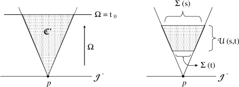
Figure 2:

The following claim is the heart of the proof of Theorem 4.1.

Claim. The energy-momentum tensor $T$ vanishes on $\mathfrak{C}^{\prime}$.

Proof of the claim: For the time being, let $s\in(0,t_{0})$ be fixed and let ${\cal U}(t):={\cal U}(s,t)$, ${\cal S}(t):={\cal S}(s,t)$ for all $t\in(s,t_{0})$. Let $A$ be the vector field defined by $g(A,X)=T(\nabla\Omega,X)$ for all $X\in{\cal X}(\tilde{M})$, hence by Stokes theorem

$$\int\limits_{{\cal U}(t)}{\rm div}A\,\text{dv}=\int\limits_{\partial{\cal U}(t)}i_{A}\text{dv}=\int\limits_{\Sigma(s)}i_{A}\text{ dv}+\int\limits_{\Sigma(t)}i_{A}\text{dv}+\int\limits_{{\cal S}(t)}i_{A}\text{dv}.$$ (4.9)

We proceed to show the integral over the null cone portion ${\cal S}(t)$ vanishes. Thus let $x\in S$. By virtue of assumption C, it suffices to show that $T(K,K)=0$ for some null vector $K\in T_{x}\tilde{M}$. Hence let us consider a future null generator $\gamma$ of $S$ through $x$. By the Raychaudhuri equation, we have

$$\frac{d\theta}{ds}=-\textrm{Ric}({\gamma}^{\prime},{\gamma}^{\prime})-{\sigma}^{2}-\frac{1}{2}{\theta}^{2}\,,$$ (4.10)

where $\theta$ is the null expansion (or null mean curvature) of $S$. Since $S$ is totally geodesic by lemma 3.3 we must have $\theta\equiv 0$ and $\sigma\equiv 0$, thus $\textrm{Ric}(\gamma^{\prime},\gamma^{\prime})=0$. Further, since $\gamma^{\prime}$ is null the Einstein equations imply $\textrm{Ric}(\gamma^{\prime},\gamma^{\prime})=T(\gamma^{\prime},\gamma^{\prime})$, and thus $T(\gamma^{\prime},\gamma^{\prime})=0$. Hence $i_{A}\text{dv}|_{S}\equiv 0$ as desired. Thus we have

$$\int\limits_{{\cal U}(t)}\text{ div}A\,\text{dv}=\int\limits_{\Sigma(t)}T(\nabla\Omega,\nabla\Omega)\text{d}\sigma-\int\limits_{\Sigma(s)}T(\nabla\Omega,\nabla\Omega)\text{d}\sigma.$$ (4.11)

Now let $\hat{T}$ be the $(1,1)$ tensor $g$-equivalent to $T$ and let $C$ denote tensor contraction with respect to $g$. Since $A=C(\hat{T}\otimes\nabla\Omega)$ we have $\text{div}A=\text{div}T\,(\nabla\Omega)+C^{2}(\hat{T}\otimes\nabla(\nabla\Omega))$. Hence

$$\int\limits_{{\cal U}(t)}\text{div}T\,(\nabla\Omega)\text{dv}\ \ + \int\limits_{{\cal U}(t)}C^{2}(\hat{T}\otimes\nabla(\nabla\Omega))\text{dv}$$

$$= \int\limits_{\Sigma(t)}\hskip-5.69046ptT(\nabla\Omega,\nabla\Omega){\rm d}\sigma\,\text{dv}\ -\int\limits_{\Sigma(s)}\hskip-5.69046ptT(\nabla\Omega,\nabla\Omega){\rm d}\sigma$$

$$\,.$$ (4.12)

Since $\mathfrak{C}^{\prime}$ is compact, the components ${\Omega_{;\alpha}}^{;\beta}$ of $\nabla(\nabla\Omega)$ in any $g$-orthonormal frame field are bounded from above, say by $Q$. Similarly, $T(\nabla\Omega,\nabla\Omega)\geq|{T^{\alpha}}_{\beta}|$ on $\tilde{M}$ by the dominant energy condition, hence by continuity, $\lim_{z\to p}T(\nabla\Omega,\nabla\Omega)_{z}\geq\lim_{z\to p}|{T^{\alpha}}_{\beta}(z)|$ as well. Then $C^{2}(\hat{T}\otimes\nabla(\nabla\Omega))\leq P\,T(\nabla\Omega,\nabla\Omega)$ on $\mathfrak{C}^{\prime}$, where $P:=16Q$. Thus

$$\int\limits_{{\cal U}(t)}C^{2}(\hat{T}\otimes\nabla(\nabla\Omega))\text{dv}\ \ \leq\int\limits_{{\cal U}(t)}P\,T(\nabla\Omega,\nabla\Omega)\text{dv}\,.$$ (4.13)

On the other hand, the formula relating the divergence operator of two conformally related metrics $g=\Omega^{2}\tilde{g}$ in a Lorentzian manifold of dimension $n$ gives,

$$\text{div}\,T(\nabla\Omega)=\frac{1}{{\Omega}^{2}}\widetilde{\text{div}}\,T(\nabla\Omega)+\frac{n-2}{\Omega}T(\nabla\Omega,\nabla\Omega)+\frac{1}{\Omega^{3}}\widetilde{\text{Tr}}\,T.$$ (4.14)

Since the physical metric satisfies the Einstein equations, the energy-momentum tensor is divergence free. Thus $\widetilde{\text{div}}\,T(\nabla\Omega)\equiv 0$ in $\tilde{M}$. Moreover, by assumption B, $\widetilde{\text{Tr}}\ T\leq 0$, thus we deduce the inequality

$$\int\limits_{{\cal U}(t)}\text{div}T\,(\nabla\Omega)\text{dv}\ \leq\int\limits_{{\cal U}(t)}\frac{2}{\Omega}\,T(\nabla\Omega,\nabla\Omega)\text{dv}$$ (4.15)

Hence equation $(\ref{integr02})$ along with $(\ref{integr03})$ and $(\ref{enineq3})$ yield

$$\int\limits_{\Sigma(t)}\hskip-5.69046ptT(\nabla\Omega,\nabla\Omega){\rm d}\sigma-\int\limits_{\Sigma(s)}\hskip-5.69046ptT(\nabla\Omega,\nabla\Omega){\rm d}\sigma\leq\int_{s}^{t}\int\limits_{\Sigma(\tau)}\left(\frac{2}{\Omega}+P\right)\,T(\nabla\Omega,\nabla\Omega){\rm d}\sigma\,\,{\rm d}\tau.$$ (4.16)

Now, we would like to analyze the limit of both sides of relation (4.16) as $s\to 0$. Let then $p(s)\in\Sigma(s)$ be such that $T(\nabla\Omega_{z},\nabla\Omega_{z})\leq T(\nabla\Omega_{p(s)},\nabla\Omega_{p(s)})$ for all $z\in\Sigma(s)$. Such $p(s)$ always exists since $\Sigma(s)$ is compact. Thus

$$\int\limits_{\Sigma(s)}\frac{1}{\Omega}T(\nabla\Omega,\nabla\Omega){\rm d}\sigma \leq \frac{1}{s}T({\nabla\Omega}_{p(s)},{\nabla\Omega}_{p(s)})\int\limits_{\Sigma(s)}\text{d}\sigma$$ (4.17)

$$= \frac{1}{s}T({\nabla\Omega}_{p(s)},{\nabla\Omega}_{p(s)})\text{Vol}(\Sigma(s))$$

Let us consider now a small normal neighborhood ${\cal N}$ around $p$. It is known [23] that the metric volume of the local causal cone truncated by a timelike vector is of the same order as the volume of the corresponding truncated cone in $T_{p}M$. Hence by considering $s$ very small we get the estimate

$$\text{Vol}(\Sigma(s))=O(s^{3}).$$ (4.18)

Thus without loss of generality we can take $t_{0}>0$ such that $\mathfrak{C}^{\prime}$ is contained in such a normal neighborhood ${\cal N}$. Thus, for $s$ sufficiently small, (4.17) and (4.18) imply,

$$\int\limits_{\Sigma(s)}\frac{1}{\Omega}T(\nabla\Omega,\nabla\Omega){\rm d}\sigma\leq C\,T({\nabla\Omega}_{p(s)},{\nabla\Omega}_{p(s)})s^{2}$$ (4.19)

for some positive constant $C$. Hence

$$\lim_{s\to 0^{+}}\int\limits_{\Sigma(s)}\frac{1}{\Omega}T(\nabla\Omega,\nabla\Omega){\rm d}\sigma=0$$ (4.20)

by virtue of assumption D.

Let $x=x(t)$ be the function defined by,

$$x(t):=\int_{0}^{t}\int\limits_{\Sigma(\tau)}\left(\frac{2}{\Omega}+P\right)T(\nabla\Omega,\nabla\Omega){\rm d}\sigma\,\,{\rm d}\tau\,,$$ (4.21)

which makes sense since, by (4.20), the integrand continuously extends to $\tau=0$. By letting $s\to 0^{+}$ in inequality (4.16) we obtain,

$$\int\limits_{\Sigma(t)}\hskip-5.69046ptT(\nabla\Omega,\nabla\Omega){\rm d}\sigma\leq x(t)\,.$$ (4.22)

Differentiation of (4.21) for $t\in(0,t_{0})$ gives,

$$\frac{dx}{dt}=\left(\frac{2}{t}+P\right)\int\limits_{\Sigma(t)}\hskip-5.69046ptT(\nabla\Omega,\nabla\Omega){\rm d}\sigma$$ (4.23)

which when combined with (4.22) yields the differential inequality,

$$\frac{d}{dt}\left(\frac{e^{-Pt}}{t^{2}}x\right)\leq 0\,.$$ (4.24)

Hence the function

$$I(t)=\frac{x(t)e^{-Pt}}{t^{2}}$$ (4.25)

is decreasing near ${\cal J}^{-}$.

Thus, we analyze ${\displaystyle\lim_{t\to 0^{+}}I(t)}$. Notice first that estimate (4.19) yields

$$\int\limits_{\Sigma(t)}\left(\frac{2}{\Omega}+P\right)T(\nabla\Omega,\nabla\Omega){\rm d}\sigma\leq C^{\prime}\,T(\nabla\Omega_{p(t)},\nabla\Omega_{p(t)})t^{2}$$ (4.26)

for some constant $C^{\prime}\geq 0$. Thus we get

$$\lim_{t\to 0^{+}}\frac{x(t)}{{t}^{2}} = \lim_{t\to 0^{+}}\frac{1}{2{t}}\int\limits_{\Sigma(t)}\left(\frac{2}{\Omega}+P\right)T(\nabla\Omega,\nabla\Omega){\rm d}\sigma$$

$$\leq \frac{C^{\prime}}{2}\,t\,T(\nabla\Omega_{p(t)},\nabla\Omega_{p(t)})\,,$$

which, by condition D implies that ${\displaystyle\lim_{t\to 0^{+}}\frac{x(t)}{{t}^{2}}}=0$, and hence ${\displaystyle\lim_{t\to 0^{+}}I(t)}=0$. It follows that $I(t)\equiv 0$ on $\mathfrak{C}^{\prime}$, and consequently $T(\nabla\Omega,\nabla\Omega)\equiv 0$ on $\mathfrak{C}^{\prime}$. Therefore $T\equiv 0$ on $\mathfrak{C}^{\prime}$ by the dominant energy condition. This completes the proof of the claim.

Now let $0<t_{1}<t_{0}$ and let $(N,h)$ be a globally hyperbolic extension of $(M,g)$. Further, let $\mathfrak{C}^{\prime\prime}:=\mathfrak{C}\cap\Omega^{-1}([0,t_{1}])$ and let us denote by ${\cal S}^{+}$ the portion of $N_{p}$ to the future of $\Sigma(t_{1})$. Hence it is clear that $T\equiv 0$ on $\mathfrak{C}^{\prime\prime}$. Further, let $x$ be in the topological interior of $D^{+}({\cal S}^{\prime},N)$, hence $W=J^{-}(x,N)\cap J^{+}({\cal S}^{\prime},N)$ is compact. Then $T\equiv 0$ on $W$ by the conservation theorem of Hawking and Ellis (cfr. page 93 in [15]), thus $T\equiv 0$ on $\text{int}D^{+}({\cal S}^{\prime},N)$. Hence by continuity we have $T\equiv 0$ on $D^{+}({\cal S}^{\prime},N)\cap\tilde{M}$.

On the other hand, let $x\in J^{+}(p,N)\cap\tilde{M}-\mathfrak{C}^{\prime\prime}$ and let $\gamma$ be a past inextendible timelike curve with future endpoint $x$. Since $J^{+}(p,N)\cap\tilde{M}\subset D^{+}(N_{p},N)\tilde{M}$ by lemma 3.2, we have that $\gamma$ must intersect $N_{p}$, say at $y$. If $\Omega(y)\geq t_{1}$ then $y\in{\cal S}^{\prime}$. If $\Omega(y)<t_{1}$ then notice that $\Omega(x)>t_{1}$ since $x\not\in\mathfrak{C}^{\prime\prime}$. Now, since the function $t\mapsto\Omega(\gamma(t))$ is continuous there exist a point $z\in\gamma$ between $x$ and $y$ such that $\Omega(z)=t_{1}$. Hence $z\in\Sigma(t_{1})\subset{\cal S}^{\prime}$. Thus we have the inclusions $I^{+}(S)\subset J^{+}(p,N)\cap\tilde{M}\subset\mathfrak{C}^{\prime\prime}\cup(D^{+}({\cal S}^{\prime},N)\cap\tilde{M})$ where $S=\partial I^{+}(\eta)$ as in lemma 3.3. Then we just showed $T\equiv 0$ on $I^{+}(S)$.

In a time dual fashion, we can show $T$ vanishes in a neighborhood of $q$ and consequently on the whole set $I^{-}(S)$. To finish the proof, recall that since $\partial I^{+}(\eta)=S=\partial I^{-}(\eta)$ then $\tilde{M}=S\cup I^{+}(S)\cup I^{-}(S)$, therefore $T\equiv 0$ on $\tilde{M}$ and the result follows. $\Box$

We conclude with a couple of remarks. In [11, 12], a uniqueness result for Minkowski space is obtained that is entirely analogous to theorem 1.1. Although, in the asymptotically Minkowskian setting, the fact that ${\cal J}$ is null adds some complications to the analysis, one should still be able to modify the techniques used here to allow a priori for the presence of matter in that setting, as well. Also, note that Maxwell fields are excluded from theorem 4.1; they do not satisfy condition C. Nonetheless, by taking advantage of the conformal invariance of such fields, it may be possible to obtain a version of theorem 4.1 that includes them.

References

- [1]
- [2] L. Andersson and G. J. Galloway. DS/CFT and spacetime topology. Adv. Theor. Math. Phys. 6 (2002) 307-327.
- [3] I. Bengtsson and S. Holst. De Sitter space and spatial topology. Class. Quantum Grav. 16 (1999) 3735-3748.
- [4] A. Bernal and M. Sánchez. Smoothness of time functions and the metric splitting of globally hyperbolic spacetimes. Comm. Math. Phys. 257 (2005) 43-50.
- [5] R. Bousso. Adventures in de Sitter space in The Future of Theoretical Physics and Cosmology. Eds. G. W. Gibbons, E. P. Shellard and S. J. Rankin. (Cambridge University Press, Cambridge, 2003).
- [6] R. Budic et al. On the determination of Cauchy surfaces from intrinsic properties. Commun. Math. Phys. 61 (1978) 87-95.
- [7] J. Cheeger and D. Ebin. Comparison Theorems in Riemannian Geometry. (Noth-Holland, Amsterdam, 1975).
- [8] Y. Choquet-Bruhat and R. Geroch. Global aspects of the Cauchy problem in general relativity. Commun. Math. Phys. 14 (1969) 329-335.
- [9] H. Friedrich. Existence and strcture of past asymptotically simple solutions of Einstein’s field equations with positive cosmological constant. J. Geom. Phys. 3 (1986) 101-117.
- [10] H. Friedrich. On the existence of -geodesically complete solutions of Einstein’s field equations with smooth asymptotic structure. Comm. Math. Phys. 107 (1986) 587-609.
- [11] G. J. Galloway. Maximum principles for null hypersurfaces and null splitting theorems. Ann. Henri Poincare 1 no. 3, (2000) 543-567.
- [12] G. J. Galloway. Some global results for asymptotically simple space-times in: The conformal Structure of Space-times; Geometry, Analysis, Numerics. Eds. J. Frauendiener and H. Friedrich. Lecture Notes in Physics, vol. 604 (Springer Verlag, New York, 2002).
- [13] G. J. Galloway. Null geometry and the Einstein equations in: The Einstein Equations and the Large Scale Behavior of Gravitational Fields. Eds. P. T. Chrusciel and H. Friedrich (Birkhauser, 2004).
- [14] S. Gao and R. Wald. Theorems on gravitational delay and related issues. Class. Quantum Grav. 17 (2000) 4999-5008.
- [15] S. W. Hawking and G. F. R. Ellis. The Large Scale Structure of Space-time. (Cambridge University Press, Cambridge, 1973).
- [16] M. Kriele. Spacetime. Foundations of General Relativity and Differential Geometry. Lecture Notes in Physics, Vol. m59. (Springer Verlag, New York, 2001).
- [17] J. M. Lee. Introduction to Smooth Manifolds. Graduate Texts in Mathematics, vol 218. (Springer Verlag, New York, 2002).
- [18] G. Mess. Lorentz spacetimes of constant curvature. preprint IHES/M/90/28 (1990).
- [19] B. O’Neill Semi-Riemannian Geometry, with Applications to Relativity. (Academic Press, London, 1983).
- [20] R. Penrose. Zero rest-mass fileds includig gravitation: asymptotic behavior. Proc. Roy. Soc. Lond. A 284 (1965) 159-203.
- [21] R. Penrose. Techniques of Differential Topology in Relativity. Regional Conference Series in Applied Mathematics, vol. 7. (SIAM, Philadelphia, 1972).
- [22] R. K. Sachs and H. Wu. General Relativity for Mathematicians. Graduate Texts in Mathematics, Vol. 48. (Springer Verlag, New York, 1977).
- [23] R. Schimming and S. Matel-Kaminska. The volume problem for pseudo-Riemannian manifolds. Z. Anal. Anwendungen. 9 (1990) 3-14.
- [24] M. Spivak A Comprehensive Introduction to Differential Geometry. vol. 5. Second Edition. (Publish or Perish, Delaware, 1979).
- [25] R. Wald. General Relativity. (The University of Chicago Press, Chicago, 1984).