Improved outer boundary conditions for Einstein’s field equations

Abstract

In a recent article, we constructed a hierarchy ${\cal B}_{L}$ of outer boundary conditions for Einstein’s field equations with the property that, for a spherical outer boundary, it is perfectly absorbing for linearized gravitational radiation up to a given angular momentum number $L$. In this article, we generalize ${\cal B}_{2}$ so that it can be applied to fairly general foliations of spacetime by space-like hypersurfaces and general outer boundary shapes and further, we improve ${\cal B}_{2}$ in two steps: (i) we give a local boundary condition ${\cal C}_{2}$ which is perfectly absorbing including first order contributions in $2M/R$ of curvature corrections for quadrupolar waves (where $M$ is the mass of the spacetime and $R$ is a typical radius of the outer boundary) and which significantly reduces spurious reflections due to backscatter, and (ii) we give a non-local boundary condition ${\cal D}_{2}$ which is exact when first order corrections in $2M/R$ for both curvature and backscatter are considered, for quadrupolar radiation.

I Introduction and main results

Most often, numerical simulations of black hole spacetimes involve replacing the physical unbounded domain with a compact domain $\Sigma$ with artificial outer boundary $\partial\Sigma$. In order to obtain a well-defined Cauchy evolution, boundary conditions need to be specified at $\partial\Sigma$. Ideally, these conditions should be formulated in such a way that the artificial boundary is completely transparent to the physical problem on the unbounded domain. However, in reality, one aims for boundary conditions which (i) form a well-posed initial boundary value problem (IBVP) and (ii) insure that very little spurious reflection of gravitational radiation occurs from the outer boundary. Boundaries which meet these two criteria are called absorbing.

The formulation of absorbing outer boundary conditions in general relativity has always been a challenging problem, primarily because constraint violations can enter the numerical domain via the outer boundary, the definition of in- and outgoing radiation is ambiguous, and the evolution of the geometry of the outer boundary is not known a priori. Strides towards the development of absorbing outer boundaries which both preserve the constraints and control the gravitational radiation by freezing the Newman-Penrose Weyl scalar $\Psi_{0}$ to its initial value have been made in Refs. [1, 2, 3, 4, 5, 6]. For other approaches which preserve the constraints exactly but control the radiation at the boundary through different means, see Refs. [7, 8, 9, 10]. In [11], boundary conditions which are perfectly absorbing for quadrupolar solutions of the flat wave equation are analyzed and numerically implemented via spectral methods, and proposed to be used in a constrained evolution scheme of Einstein’s field equations [12]. Other methods avoid introducing an artificial outer boundary altogether by compactifying spatial infinity [13, 14] or by making use of hyperboloidal slices and compactifying null infinity (see, for instance [15, 16, 17]).

Recently, a hierarchy ${\cal B}_{L}$ of local boundary conditions for $\Psi_{0}$ has been proposed (see Eq. (128) of [18]) which, for $L\geq 2$, improves the freezing $\Psi_{0}$ boundary condition given in [1, 2, 3, 4, 5, 6] in that it is perfectly absorbing on a spherical boundary for linearized gravitational perturbations with angular momentum number $\ell\leq L$. If the outer boundary is placed in the wave zone (meaning $kR\gg 1$, where $R$ is a characteristic radius of the outer boundary and $k$ is the characteristic wave number) and the solution is smooth enough, the few lower $\ell$ multipoles will dominate. Therefore, the boundary condition ${\cal B}_{L}$ with $L=2,3$ or $4$ should yield very little spurious reflections in linearized gravity. When considering the full nonlinear problem, if the outer boundary is not only in the wave zone but also far away from the strong field region (meaning $R\gg M$ where $M$ is the total mass of the system, that is, the Arnowitt-Deser-Misner (ADM) mass), one expects the spacetime to be described by a linear perturbation about Minkowski spacetime. Therefore, in the nonlinear case, the boundary conditions ${\cal B}_{L}$ for $L=2,3$ or $4$ should also yield small spurious reflections provided that $kR\gg 1$ and $R\gg M$.

In this article, we formulate ${\cal B}_{L}$ to be applicable to more general slicings than in [18]; furthermore, we construct ${\cal B}_{L}$ in such a way that the outer boundary is not restricted to be an approximate metric sphere. The approach we adopt is to describe a general four dimensional metric near the outer boundary of the computational domain as the Schwarzschild metric plus a perturbation. We perturb Schwarzschild, rather than Minkowski, spacetime in order to incorporate leading order effects in $M/R$ into our boundary conditions. For an asymptotically flat spacetime, the $M/R$ correction terms to Minkowski spacetime are given by the monopole contribution of the Schwarzschild metric. When these terms are taken into account, a gravitational wave solution on Minkowski spacetime acquires two types of correction terms. The first is the curvature correction term which obeys Hugyens’ principle and the second is a fast decaying term which violates Hugyens’ principle and describes the backscatter off of curvature.

A method which provides exact outer boundary conditions for linearized waves propagating on a Schwarzschild background has been recently presented in [19, 20, 21]. However, in view of the nonlinear theory, there is no advantage to obtaining a boundary condition which takes into account the exact form of the Schwarzschild metric beyond the order of $M/R$, since the full spacetime agrees with the Schwarzschild metric only up to order $M/R$. If second order effects are to be taken into account, then linear effects in $J/R^{2}$ (where $J$ is the total angular momentum of the system) and quadratic effects in $M/R$ from the full metric should also be included.

Our boundary conditions ${\cal B}_{L}$ are formulated as follows. We assume that in the vicinity of the outer boundary, the spacetime metric is the Schwarzschild metric of mass $M$ plus a small perturbation of it. More precisely, we assume that the spacetime manifold near the outer boundary can be written locally as a product of a two-dimensional manifold $\tilde{\cal M}$ and a unit two-sphere $S^{2}$ such that if $(x^{a})$ denote local coordinates on $\tilde{M}$ and $(x^{A})=(\vartheta,\varphi)$ denote the usual angular coordinates on $S^{2}$, the components of the full metric $g^{(full)}$ satisfy the following conditions:

$$|g^{(full)}_{ab}-\tilde{g}_{ab}|\ll 1,\qquad|g^{(full)}_{aB}|\ll 1,\qquad|g^{(full)}_{AB}/r^{2}-\hat{g}_{AB}|\ll 1,$$ (1)

where $\hat{g}=d\vartheta^{2}+\sin^{2}\vartheta d\varphi^{2}$ is the standard metric on $S^{2}$, $r$ is the areal radius, and $\tilde{g}$ is a pseudo-Riemannian metric on $\tilde{M}$ representing the radial part of the background Schwarzschild metric. In standard Schwarzschild coordinates $(t,r)$, we have $\tilde{g}=-N(r)dt^{2}+N(r)^{-1}dr^{2}$, where $N=1-2M/r$. However, we do not assume that $(x^{a})$ are Schwarzschild coordinates: with respect to the coordinates $(x^{a})$ on $\tilde{M}$, the components of $\tilde{g}$ are given by the coordinate transformation of the $(t,r)$-components of $\tilde{g}$ which minimizes $|g_{ab}^{(full)}-\tilde{g}_{ab}|$. If the boundary is spherical, a natural representation of the spacetime manifold in the neighborhood of the outer boundary as $\tilde{M}\times S^{2}$ exists, and our hope is that one can enforce clever boundary conditions on the gauge degrees of freedom guaranteeing that conditions (1) are satisfied. In this case, a method for computing $r$ and $\tilde{g}$ from the full metric is the following [22]: if $\sigma_{ab}=g^{(full)}_{ab}$ and $\gamma_{AB}=g^{(full)}_{AB}$ denote the induced metrics on $\tilde{\cal M}$ and $S^{2}$, respectively, then $r$ is defined by $4\pi r^{2}=\int_{S^{2}}\sqrt{|\gamma|}\sin(\vartheta)d\vartheta d\varphi$ and $\tilde{g}:=\int_{S^{2}}\sigma\sin(\vartheta)d\vartheta d\varphi$. If the boundary is not spherical, $\tilde{g}$ and $r$ need to be computed by other methods: a possible approach is to use a minimization technique in order to optimize the inequalities in (1).

Having identified $\tilde{M}$, $\tilde{g}$ and $r$, one introduces the coordinates $t$ and $r_{*}$ on $\tilde{\cal M}$ which correspond to the Schwarzschild time and tortoise coordinates, respectively, but which are defined in a completely geometric way (see Section II) so that different observers on $\tilde{M}$ agree on their definition. Consequently, the boundary condition ${\cal B}_{L}$ does not depend on the foliation of $\tilde{M}$. It reads

$${\cal B}_{L}:~{}~{}~{}~{}~{}\left.\partial_{t}\left[r^{2}(\partial_{t}+\partial_{r_{*}})\right]^{L-1}\left(r^{5}\Psi_{0}\right)\right|_{\partial\Sigma}=0,$$ (2)

where the Weyl scalar $\Psi_{0}$ is defined in terms of the Newman-Penrose null tetrad given in Sect. II. Notice that ${\cal B}_{1}$ is the freezing $\Psi_{0}$ boundary condition.

After formulating ${\cal B}_{L}$, we concentrate on improving ${\cal B}_{2}$ by reducing spurious reflections off the outer boundary due to curvature corrections and backscatter. We accomplish this by computing in- and outgoing quadrupolar solutions for even and odd-parity perturbations of the Schwarzschild metric $\tilde{g}+r^{2}\hat{g}$, to first order in $2M/R$. Using these approximate solutions, we compute reflection coefficients which quantify the amount of spurious reflections. When calculating the reflection coefficients, we assume for simplicity that the outer boundary is an approximate metric sphere with constant area $4\pi R^{2}$. This allows us to compare the amount of reflections resulting from our improved boundary conditions with those resulting from ${\cal B}_{1}$, for a spherical outer boundary. Our boundary condition ${\cal B}_{2}$ already gives a $1.2(M/R)(kR)^{-1}$ times reduction in the amount of spurious reflections compared to ${\cal B}_{1}$ for $kR>1.05$. We find we can improve ${\cal B}_{2}$, however, by applying the operator in Eq. (2) to $r^{5}N^{-1}\Psi_{0}$ rather than to $r^{5}\Psi_{0}$ (recall $N=1-2M/r$) giving

$${\cal C}_{2}:~{}~{}~{}~{}~{}\left.\partial_{t}(\partial_{t}+\partial_{r_{*}})\left(r^{5}N^{-1}\Psi_{0}\right)\right|_{\partial\Sigma}=0.$$ (3)

For a spherical outer boundary, ${\cal C}_{2}$ reduces spurious reflections due to curvature corrections and backscatter by a factor of $(15M/2R)(kR)^{-2}$ compared to ${\cal B}_{1}$, for $kR>1$. We have not calculated the reflection coefficients for boundary shapes other than spherical; however, we stress that our boundary conditions ${\cal B}_{L}$ and ${\cal C}_{2}$ can be applied to general outer boundary shapes. Furthermore, we show that in general, $C_{2}$ is perfectly absorbing to first order in $2M/R$ if backscatter is neglected but the curvature correction terms are taken into account.

Finally, we improve ${\cal C}_{2}$ so that it is perfectly absorbing up to order $2M/R$ including backscatter for quadrupolar gravitational radiation. This boundary condition reads

$${\cal D}_{2}:~{}~{}~{}~{}~{}\left[r(\partial_{t}+\partial_{r_{*}})\left(r^{5}N^{-1}\Psi_{0}\right)+\frac{30M}{r}\int\limits_{0}^{t/2r}\frac{r^{5}\Psi_{0}(t-2ry,r,\vartheta,\varphi)dy}{(1+y)^{7}}\right]_{\partial\Sigma}=G,$$ (4)

where $G$ is some appropriate boundary data which can be computed from the portion of the initial data which is exterior to the outer boundary (see Eq. (38) below). In particular, $G=0$ if the initial data vanish in the region exterior the the outer boundary.

Our article is organized as follows. In Sect. II, first we consider an arbitrary spherically symmetric background manifold of the form $\tilde{\cal M}\times S^{2}$ and show how, in vacuum, the coordinates $t$ and $r_{*}$ can be defined in a geometric way. This definition is important as it makes it possible to apply our boundary conditions to quite general foliations of the spacetime and to spherical as well as non-spherical outer boundary shapes. Next, using the gauge-invariant perturbation formalism presented in [23], we derive the linearized Weyl scalars $\delta\Psi_{0}$ and $\delta\Psi_{4}$ when there are both even and odd-parity perturbations on a Schwarzschild background in arbitrary spherically symmetric coordinates. These scalars are invariant with respect to infinitesimal coordinate transformations and tetrad rotations, and we use $\delta\Psi_{0}$ to construct our new boundary conditions. In Sect. III, we compute the in- and outgoing quadrupolar solutions to the Regge-Wheeler and Zerilli equations up to order $2M/R$. Here, we find the interesting result that for the perturbed Weyl scalar $\delta\Psi_{0}$, the ingoing solutions are identical for both the even and odd-parity sectors, whereas the outgoing solutions for these sectors differ by a sign in a first order correction term. In Sect. IV, we discuss the boundary conditions ${\cal B}_{2}$ and ${\cal C}_{2}$ and calculate the corresponding reflection coefficients up to first order corrections in $2M/R$. For ${\cal B}_{2}$, the reflection coefficient decays as $(2M/R)(kR)^{-5}$ and for ${\cal C}_{2}$, it decays as $(2M/R)(kR)^{-6}$ (for $kR\gg 1$). Finally, we construct the boundary condition ${\cal D}_{2}$, which is perfectly absorbing including backscatter and curvature correction terms, to first order in $2M/R$. Conclusions are drawn in Sect. V where we also present the boundary condition ${\cal C}_{L}$ [24], a generalization of ${\cal C}_{2}$ derived from the results in [25]. In the appendix, we analyze the stability of the boundary condition ${\cal D}_{2}$ for a related model problem.

II Linear perturbations of a spherically symmetric vacuum spacetime

In this section, we first consider an arbitrary spherically symmetric background spacetime which can be represented as the product of a two-manifold $\tilde{\cal M}$ and a two-sphere $S^{2}$ and show how the coordinates $t$ and $r_{*}$ on $\tilde{M}$ can be defined geometrically, provided that the background spacetime satisfies Einstein’s vacuum equations. We then use the perturbation formalism in [23], which is a generalization of the Regge-Wheeler [26] and Zerilli [27] equations to arbitrary spherically symmetric coordinates, to derive formulas for calculating the linearized Weyl scalars $\delta\Psi_{0}$, $\delta\Psi_{4}$, and $\mbox{Im}(\delta\Psi_{2})$. As constructed in this section, these Weyl scalars are gauge-invariants in the sense that they are invariant with respect to infinitesimal coordinate transformations and tetrad rotations.

The generalized Regge-Wheeler and Zerilli equations found in [23] have the form of wave equations with potentials for the gauge-invariant scalars $\Phi^{(-)}_{\ell m}$ and $\Phi^{(+)}_{\ell m}$ which describe, respectively, odd and even-parity linear fluctuations of the background geometry with angular momentum numbers $\ell m$. In [23], it was also shown that the complete set of metric perturbations in the Regge-Wheeler gauge can be reconstructed from the scalars $\Phi^{(-)}_{\ell m}$ and $\Phi^{(+)}_{\ell m}$ without solving additional differential equations. In particular, the linearized Weyl scalars $\delta\Psi_{0}$, $\delta\Psi_{4}$ and $\mbox{Im}(\delta\Psi_{2})$, which are gauge-invariant quantities, are entirely determined by these scalars.

II.1 Background equations

We consider a spherically symmetric background of the $2+2$ form $\tilde{M}\times S^{2}$ with metric

$$g=\tilde{g}_{ab}\,dx^{a}dx^{b}+r^{2}\,\hat{g}_{AB}\,dx^{A}dx^{B},$$ (5)

where $\hat{g}=d\vartheta^{2}+\sin^{2}\vartheta d\varphi^{2}$ is the standard metric on $S^{2}$ and $\tilde{g}$ and $r$ denote the metric tensor and a positive function, respectively, defined on the two-dimensional pseudo-Riemannian orbit space $\tilde{M}$. In what follows, lower-case Latin indices refer to coordinates on $\tilde{M}$, while capital Latin indices refer to the coordinates $\vartheta$ and $\varphi$ on $S^{2}$. The $ab$ components of the Einstein tensor belonging to the metric (5) are

$$G_{ab}=-\frac{2}{r}\tilde{\nabla}_{a}\tilde{\nabla}_{b}r+\frac{1}{r^{2}}\tilde{g}_{ab}\left(2r\tilde{\Delta}r+N-1\right),$$ (6)

where $\tilde{\nabla}$ denotes the covariant derivative compatible with $\tilde{g}$, $\tilde{\Delta}\equiv\tilde{\nabla}^{a}\tilde{\nabla}_{a}$ and $N=\tilde{g}(dr,dr)=\tilde{g}^{ab}\tilde{\nabla}_{a}r\cdot\tilde{\nabla}_{b}r$. A coordinate-invariant definition of the ADM mass is given by

$$M=\frac{r}{2}(1-N).$$ (7)

In vacuum, Eq. (6) yields

$$\tilde{\nabla}_{a}\tilde{\nabla}_{b}r=\frac{M}{r^{2}}\tilde{g}_{ab}\;.$$ (8)

Eqs. (7) and (8) imply that $M$ is constant.

For the following, we assume that $N>0$. Since in this article we are interested in the asymptotic regime of the Schwarzschild spacetime, where $N$ is close to one, this assumption poses no problems. The two vector fields

$$t^{a}=-\tilde{\varepsilon}^{ab}\tilde{\nabla}_{b}r,\qquad r^{a}=\tilde{\nabla}^{a}r$$ (9)

on $\tilde{M}$, where $\tilde{\varepsilon}_{ab}$ denotes the natural volume element on $\tilde{M}$, are orthogonal to each other and are linearly independent since $r_{a}r^{a}=-t_{a}t^{a}=N>0$. As a consequence of Eq. (8), $\tilde{\nabla}_{a}t_{b}=M\tilde{\varepsilon}_{ab}/r^{2}$; hence, $t^{a}$ is a Killing vector field. Furthermore, it follows from (8) that $t^{a}$ and $r^{a}$ commute. Therefore, it is possible to introduce coordinates $(t,r_{*})$ on $\tilde{M}$ such that $t^{a}\partial_{a}=\partial_{t}$ and $r^{a}\partial_{a}=\partial_{r_{*}}$. The coordinates $t$ and $r_{*}$ correspond to the standard Schwarzschild time and tortoise coordinates, respectively. For later use, we also introduce the two null vector fields

$$l^{a}\partial_{a} = \frac{1}{\sqrt{2N}}\left(t^{a}+r^{a}\right)\partial_{a}=\frac{1}{\sqrt{2N}}(\partial_{t}+\partial_{r_{*}}),$$ (10)

$$k^{a}\partial_{a} = \frac{1}{\sqrt{2N}}\left(t^{a}-r^{a}\right)\partial_{a}=\frac{1}{\sqrt{2N}}(\partial_{t}-\partial_{r_{*}}),$$ (11)

satisfying $\tilde{g}_{ab}=-l_{a}k_{b}-k_{a}l_{b}$ and $\tilde{\varepsilon}_{ab}=l_{a}k_{b}-k_{a}l_{b}$. They can be completed to form a Newman-Penrose null tetrad $\{l^{a},k^{a},m^{B},\bar{m}^{B}\}$, where $m^{B}$ is a complex null vector field and $\bar{m}^{B}$ its complex conjugate such that $r^{2}\hat{g}_{AB}=m_{A}\bar{m}_{B}+\bar{m}_{A}m_{B}$ and the volume element $\hat{\varepsilon}$ belonging to $\hat{g}$ is given by $r^{2}\hat{\varepsilon}_{AB}=i(m_{A}\bar{m}_{B}-\bar{m}_{A}m_{B})$. The Weyl scalars are defined as

$$\Psi_{0} = C_{\alpha\beta\mu\nu}l^{\alpha}m^{\beta}l^{\mu}m^{\nu},$$

$$\Psi_{1} = C_{\alpha\beta\mu\nu}l^{\alpha}k^{\beta}l^{\mu}m^{\nu},$$

$$\Psi_{2} = C_{\alpha\beta\mu\nu}l^{\alpha}m^{\beta}\bar{m}^{\mu}k^{\nu},$$

$$\Psi_{3} = C_{\alpha\beta\mu\nu}l^{\alpha}k^{\beta}k^{\mu}\bar{m}^{\nu},$$

$$\Psi_{4} = C_{\alpha\beta\mu\nu}k^{\alpha}\bar{m}^{\beta}k^{\mu}\bar{m}^{\nu},$$

where $C_{\alpha\beta\mu\nu}$ denotes the Weyl tensor. For a spherically symmetric spacetime of the form (5) with the tetrad choice (10,11), all the Weyl scalars vanish except for

$$\Psi_{2}=-\frac{M}{r^{3}}\;.$$

II.2 Perturbation equations

Next, let us consider a generic linear perturbation of the background metric:

$$\delta g_{ab}=L_{ab}\;,\qquad\delta g_{aB}=Q_{aB}\;,\qquad\delta g_{AB}=r^{2}K_{AB}\;,$$

where the quantities $L_{ab}$, $Q_{aB}$ and $K_{AB}$ depend on the coordinates $(x^{a},x^{B})$. With respect to an infinitesimal coordinate transformation $\delta x^{a}\mapsto\delta x^{a}+\xi^{a}$, $\delta x^{B}\mapsto\delta x^{B}+\eta^{B}$, these quantities transform according to

$$L_{ab} \mapsto L_{ab}+2\tilde{\nabla}_{(a}\xi_{b)}\;,$$ (12)

$$Q_{aB} \mapsto Q_{aB}+\hat{\nabla}_{B}\xi_{a}+r^{2}\tilde{\nabla}_{a}\hat{\eta}_{B}\,,$$ (13)

$$K_{AB} \mapsto K_{AB}+\frac{2}{r}\,\hat{g}_{AB}\,r^{a}\xi_{a}+2\hat{\nabla}_{(A}\hat{\eta}_{B)}\,,$$ (14)

where $\hat{\nabla}$ denotes the covariant derivative compatible with $\hat{g}$ and where $\hat{\eta}_{A}\equiv\hat{g}_{AB}\eta^{B}$. A lengthy but straightforward calculation yields the following expressions for the perturbed Weyl scalars $\delta\Psi_{0}$ and $\delta\Psi_{4}$:

$$\delta\Psi_{0}=V_{abCD}l^{a}l^{b}m^{C}m^{D},\qquad\delta\Psi_{4}=V_{abCD}k^{a}k^{b}\bar{m}^{C}\bar{m}^{D},$$ (15)

where $V_{abCD}$ is given by

$$V_{abCD}=\frac{1}{2}\left(-\hat{\nabla}_{C}\hat{\nabla}_{D}L_{ab}+\hat{\nabla}_{C}\tilde{\nabla}_{(a}Q_{b)D}+\hat{\nabla}_{D}\tilde{\nabla}_{(a}Q_{b)C}-\tilde{\nabla}_{(a}r^{2}\tilde{\nabla}_{b)}K_{CD}\right)^{tf}$$ (16)

and where the superscript $tf$ refers to the trace-free part with respect to the metric $\hat{g}_{CD}$. It can be verified readily that $V_{abCD}$ is invariant with respect to the infinitesimal coordinate transformations given in Eqs. (12,13,14). Furthermore, since $\delta\Psi_{0}$ and $\delta\Psi_{4}$ do not depend on the perturbed tetrad components, they are also invariant with respect to infinitesimal tetrad rotations. In fact, this invariance of $\delta\Psi_{0}$ and $\delta\Psi_{4}$ holds for any type D background metric [28].

Since the background metric is spherically symmetric, it is convenient to expand the fields in spherical harmonics. In the resulting perturbation equations, pieces belonging to different angular momentum numbers $\ell$ and $m$ decouple. Thus, it is sufficient to consider one fixed value of $\ell$ and $m$ at a time. The decomposition of the fields $L_{ab}$, $Q_{aB}$ and $K_{AB}$ into tensor spherical harmonics reads

$$L_{ab} = H_{ab}Y,$$

$$Q_{aB} = Q_{a}\hat{\nabla}_{B}Y+h_{a}\hat{S}_{B}\,,$$ (17)

$$K_{AB} = K\hat{g}_{AB}Y+G\left[\hat{\nabla}_{A}\hat{\nabla}_{B}\right]^{tf}Y+2k\hat{\nabla}_{(A}\hat{S}_{B)}\,,$$

where $Y=Y^{\ell m}(\vartheta,\varphi)$ denotes the standard spherical harmonics and $\hat{S}_{A}\equiv\hat{\varepsilon}_{A}{}^{B}\hat{\nabla}_{B}Y$. With respect to this, we obtain

$$V_{abCD}=-\frac{1}{2}H_{ab}^{(inv)}\left[\hat{\nabla}_{C}\hat{\nabla}_{D}\right]^{tf}Y+\tilde{\nabla}_{(a}h_{b)}^{(inv)}\hat{\nabla}_{(C}\hat{S}_{D)}\,,$$ (18)

where $H_{ab}^{(inv)}$ and $h_{b}^{(inv)}$ are the gauge-invariant amplitudes defined in [23] which, in the Regge-Wheeler gauge, reduce to the quantities $H_{ab}$ and $h_{b}$, respectively. These gauge-invariants were first given in [29]. For vacuum perturbations, these gauge-invariant quantities are entirely determined by two scalar fields $\Phi^{(+)}$ and $\Phi^{(-)}$ according to

$$H_{ab}^{(inv)} = -\frac{2}{\lambda+a_{0}}\left(\tilde{\nabla}_{a}\tilde{\nabla}_{b}-\frac{1}{2}\tilde{g}_{ab}\tilde{\Delta}\right)\left[r(\lambda+a_{0})\Phi^{(+)}\right],$$ (19)

$$h_{b}^{(inv)} = \tilde{\varepsilon}_{ab}\tilde{\nabla}^{a}\left[r\Phi^{(-)}\right],$$ (20)

where $\lambda\equiv(\ell-1)(\ell+2)$ and $a_{0}\equiv 6M/r$. The two scalar fields $\Phi^{(+)}$ and $\Phi^{(-)}$ satisfy the Zerilli [27] and Regge-Wheeler [26] equations, respectively:

$$\left[-\tilde{\nabla}^{a}\tilde{\nabla}_{a}+V_{\pm}(r)\right]\Phi^{(\pm)}=0,$$ (21)

where the potentials are given by

$$V_{+}(r) = \frac{\lambda^{2}r^{2}\left[\ell(\ell+1)r+6M\right]+36M^{2}(\lambda r+2M)}{(\lambda r+6M)^{2}r^{3}}\,,$$

$$V_{-}(r) = \frac{\ell(\ell+1)}{r^{2}}-\frac{6M}{r^{3}}\;.$$

Taking everything together, we obtain the following expressions for the perturbed Weyl scalars $\delta\Psi_{0}$ and $\delta\Psi_{4}$:

$$\delta\Psi_{0} = \frac{1}{r^{2}}\left\{\frac{1}{\lambda+a_{0}}l^{a}l^{b}\tilde{\nabla}_{a}\tilde{\nabla}_{b}\left[r(\lambda+a_{0})\Phi^{(+)}\right]+il^{a}l^{b}\tilde{\nabla}_{a}\tilde{\nabla}_{b}\left[r\Phi^{(-)}\right]\right\}\hat{m}^{C}\hat{m}^{D}\hat{\nabla}_{C}\hat{\nabla}_{D}Y,$$ (22)

$$\delta\Psi_{4} = \frac{1}{r^{2}}\left\{\frac{1}{\lambda+a_{0}}k^{a}k^{b}\tilde{\nabla}_{a}\tilde{\nabla}_{b}\left[r(\lambda+a_{0})\Phi^{(+)}\right]+ik^{a}k^{b}\tilde{\nabla}_{a}\tilde{\nabla}_{b}\left[r\Phi^{(-)}\right]\right\}\bar{\hat{m}}^{C}\bar{\hat{m}}^{D}\hat{\nabla}_{C}\hat{\nabla}_{D}Y,$$ (23)

where we have defined $\hat{m}^{A}=r\,m^{A}$, and where the scalar fields $\Phi^{(\pm)}$ satisfy Eq. (21).

Finally, we compute the imaginary part of the perturbed Weyl scalar $\delta\Psi_{2}$. One first finds

$$\mbox{Im}(\delta\Psi_{2})=-\mbox{Im}\left(W_{abCD}l^{a}k^{b}m^{C}\bar{m}^{D}\right),$$ (24)

where the quantity

$$W_{abCD}=\frac{r^{2}}{2}\left[\hat{\nabla}_{C}\tilde{\nabla}_{[a}\left(\frac{Q_{b]D}}{r^{2}}\right)-\hat{\nabla}_{D}\tilde{\nabla}_{[a}\left(\frac{Q_{b]C}}{r^{2}}\right)\right]$$ (25)

is invariant with respect to the infinitesimal coordinate transformations given in Eqs. (12,13,14). Next, application of the decomposition (17) yields

$$W_{abCD}=r^{2}\tilde{\nabla}_{[a}\left(\frac{h^{(inv)}_{b]}}{r^{2}}\right)\hat{\nabla}_{[C}\hat{S}_{D]}\,.$$

Using Eq. (20) and $2r^{2}m^{C}\bar{m}^{D}\hat{\nabla}_{[C}\hat{S}_{D]}=i\hat{g}^{CD}\hat{\nabla}_{C}\hat{\nabla}_{D}Y$, we then obtain

$$\mbox{Im}(\delta\Psi_{2})=-\frac{\ell(\ell+1)}{4r}\left[\tilde{\nabla}^{a}\tilde{\nabla}_{a}\Phi^{(-)}-\frac{2}{r^{2}}\left(1-\frac{3M}{r}\right)\Phi^{(-)}\right]Y.$$

Finally, we substitute the Regge-Wheeler equation (21) into the above expression to get

$$\mbox{Im}(\delta\Psi_{2})=-\frac{(\ell-1)\ell(\ell+1)(\ell+2)}{4r^{3}}\Phi^{(-)}Y.$$ (26)

Therefore, the gauge-invariant scalar $\Phi^{(-)}$ obeying the Regge-Wheeler equation can be interpreted as the radial part of the imaginary part of the perturbed Weyl scalar $\delta\Psi_{2}$ [30, 18]. Comparison of Eq. (26) with the quantity $\phi=r^{2}h_{0}$ defined in [18] gives the relation $2\phi=(\ell-1)\ell(\ell+1)(\ell+2)\Phi^{(-)}$. It would be nice to know what the geometric interpretation of the gauge-invariant scalar $\Phi^{(+)}$ obeying the Zerilli equation is.

III In- and outgoing quadrupolar wave solutions

In this section, we compute in- and outgoing solutions to the Zerilli and Regge-Wheeler equations. Since we are interested only in the asymptotic regime $r\simeq R$, with $R$ large compared to $M$, we compute these solutions to first order in $2M/R$. A method for performing this task is described in [18]. We start by computing the outgoing solutions. For this purpose, we introduce the outgoing Eddington-Finkelstein coordinates $(\tau,\rho)$, which are related to the geometrically defined coordinate $t$ and the areal radius $r$ of Sect. II.1 through

$$\tau=t+r-r_{*}\,,\qquad\rho=r,$$

where the tortoise coordinate $r_{*}$ is defined by $r_{*}(r)=r-4M+2M\log(r/2M-1)$. In these coordinates, the two-metric reads

$$\tilde{g}=-d\tau^{2}+d\rho^{2}+\frac{2M}{\rho}(d\tau-d\rho)^{2}.$$

With respect to this metric, the Zerilli and Regge-Wheeler equations (21) can be written as

$$\left[\partial_{\tau}^{2}-\partial_{\rho}^{2}+\frac{\ell(\ell+1)}{\rho^{2}}\right]\Phi^{(\pm)}=-\frac{2M}{\rho}\left[(\partial_{\tau}+\partial_{\rho})^{2}-\frac{1}{\rho}(\partial_{\tau}+\partial_{\rho})-\frac{3a_{\pm}}{\rho^{2}}+O\left(\frac{2M}{R}\right)\right]\Phi^{(\pm)},$$ (27)

where $a_{+}=(\lambda+4)/\lambda$ and $a_{-}=1$. In order to compute the solution to first order in $2M/R$, we make the ansatz (omitting the superscript $(\pm)$ on $\Phi$)

$$\Phi(\tau,\rho)=\Phi_{0}(\tau,\rho)+\frac{2M}{R}g_{1}(\tau,\rho),$$

where $\Phi_{0}$ is a solution of the Regge-Wheeler-Zerilli equations (21) for $2M/R=0$, and where the function $g_{1}$ satisfies the equation

$$\left[\partial_{\tau}^{2}-\partial_{\rho}^{2}+\frac{\ell(\ell+1)}{\rho^{2}}\right]g_{1}(\tau,\rho)=-\frac{R}{\rho}\left[(\partial_{\tau}+\partial_{\rho})^{2}-\frac{1}{\rho}(\partial_{\tau}+\partial_{\rho})-\frac{3a_{\pm}}{\rho^{2}}\right]\Phi_{0}\,.$$ (28)

In the following, we compute $\Phi$ for quadrupolar radiation ($\ell=2$). In this case, the outgoing flat background solution $\Phi_{0}$ is given by

$$\Phi_{0}(\tau,\rho)=U^{(2)}(\rho-\tau)-\frac{3}{\rho}U^{(1)}(\rho-\tau)+\frac{3}{\rho^{2}}U(\rho-\tau),$$

where $U$ is a smooth function on the real axis with $k$’th derivative $U^{(k)}$. In the following, we also assume that $U$ is bounded and that it vanishes for negative enough values of its argument. The corresponding solution for $g_{1}$ is given by

$$g_{1}(\tau,\rho)=\frac{3(1-a_{\pm})R}{2\rho^{3}}U(\rho-\tau)+\frac{3a_{\pm}R}{4\rho^{2}}U^{(1)}(\rho-\tau)+\frac{R}{4}\int\limits_{\rho-\tau}^{\infty}K_{2}(\tau,\rho,x)U(x)dx,$$ (29)

where the integral kernel $K_{2}$ reads

$$K_{2}(\tau,\rho,x)=\frac{3}{2\rho^{4}}\left[w^{-4}+2w^{-3}+2w^{-2}\right]_{w=\frac{\tau+\rho+x}{2\rho}}\;,\qquad x\geq\rho-\tau,$$

and satisfies

$$\left[\partial_{\tau}^{2}-\partial_{\rho}^{2}+\frac{6}{\rho^{2}}\right]K_{2}(\tau,\rho,x)=0,\qquad K_{2}(\tau,\rho,\rho-\tau)=\frac{15}{2\rho^{4}}\;.$$

The solution $g_{1}$ is not unique; one can add an arbitrary homogeneous solution of Eq. (28) to it. However, $g_{1}$ is uniquely characterized by the following conditions:

$$\lim\limits_{\rho\to\infty}g_{1}(const.+\rho,\rho)=0 \hbox{($g_{1}$ vanishes at future null infinity)},$$

$$\lim\limits_{\rho\to\infty}g_{1}(const.-\rho,\rho)=0 \hbox{($g_{1}$ vanishes at past null infinity)},$$

$$\lim\limits_{\tau\to\infty}g_{1}(\tau,const.)~{}~{}~{}~{}~{}=0 \hbox{($g_{1}$ vanishes at future time-like infinity)}.$$

Notice that the third requirement is necessary in order to exclude solutions of the form $g_{1}(\tau,\rho)=(c_{1}\tau+c_{0})\rho^{-2}$ (where $c_{0}$ and $c_{1}$ are some constants) of the zero mass Regge-Wheeler-Zerilli equations (21), which vanish at both future and past null infinity.

Summarizing, we have the following outgoing approximate solutions of the Regge-Wheeler-Zerilli equations for $\ell=2$:

$$\Phi^{(\pm)}_{\nearrow}(t,r) = U_{\pm}^{(2)}(r_{*}-t)-\frac{3}{r}U_{\pm}^{(1)}(r_{*}-t)+\frac{3}{r^{2}}U_{\pm}(r_{*}-t)$$

$$+ \frac{2M}{R}\left[\frac{3a_{\pm}R}{4r^{2}}U_{\pm}^{(1)}(r_{*}-t)+\frac{3(1-a_{\pm})R}{2r^{3}}U_{\pm}(r_{*}-t)+\frac{R}{4}\int\limits_{r_{*}-t}^{\infty}K_{2}(r-r_{*}+t,r,x)U_{\pm}(x)dx\right]+O\left(\frac{2M}{R}\right)^{2},$$

where $a_{+}=2$, $a_{-}=1$. Since the Regge-Wheeler-Zerilli equations (21) are time-symmetric, corresponding ingoing solutions are obtained from this by merely flipping the sign of $t$:

$$\Phi^{(\pm)}_{\nwarrow}(t,r) = V_{\pm}^{(2)}(r_{*}+t)-\frac{3}{r}V_{\pm}^{(1)}(r_{*}+t)+\frac{3}{r^{2}}V_{\pm}(r_{*}+t)$$

$$+ \frac{2M}{R}\left[\frac{3a_{\pm}R}{4r^{2}}V_{\pm}^{(1)}(r_{*}+t)+\frac{3(1-a_{\pm})R}{2r^{3}}V_{\pm}(r_{*}+t)+\frac{R}{4}\int\limits_{r_{*}+t}^{\infty}K_{2}(r-r_{*}-t,r,x)V_{\pm}(x)dx\right]+O\left(\frac{2M}{R}\right)^{2}.$$

Using equation (22) and the identity

$$\frac{1}{r}l^{a}l^{b}\tilde{\nabla}_{a}\tilde{\nabla}_{b}(r\Phi)=\frac{N}{2r^{4}}\left[\frac{r^{2}}{N}(\partial_{t}+\partial_{r_{*}})\right]^{2}\Phi,$$

which holds for the Schwarzschild background, we obtain the following expressions for the perturbed Weyl scalar $\delta\Psi_{0}$:

$$\delta\Psi_{0}=\frac{1}{r}\left(\psi^{(+)}_{0}+i\,\psi^{(-)}_{0}\right)\hat{m}^{C}\hat{m}^{D}\hat{\nabla}_{C}\hat{\nabla}_{D}Y,$$ (30)

where

$$\psi^{(\pm)}_{0\nearrow}(t,r) = \frac{3}{r^{4}N}\left\{U_{\pm}(r_{*}-t)+\frac{2M}{r}\left[-2U_{\pm}(r_{*}-t)\mp\frac{r}{4}U_{\pm}^{(1)}(r_{*}-t)+\frac{1}{2}\int\limits_{0}^{\infty}k(1+y)U_{\pm}(r_{*}-t+2ry)dy\right]\right.$$ (31)

$$+ \left.O\left(\frac{2M}{R}\right)^{2}\right\},$$

$$\psi^{(\pm)}_{0\nwarrow}(t,r) = \frac{3}{r^{4}N}\left\{V_{\pm}(r_{*}+t)-2rV_{\pm}^{(1)}(r_{*}+t)+2r^{2}V_{\pm}^{(2)}(r_{*}+t)-\frac{4}{3}r^{3}V_{\pm}^{(3)}(r_{*}+t)+\frac{2}{3}r^{4}V_{\pm}^{(4)}(r_{*}+t)\right.$$ (32)

$$+ \left.\frac{2M}{r}\left[\frac{1}{2}r^{2}V_{\pm}^{(2)}(r_{*}+t)-\frac{1}{2}r^{3}V_{\pm}^{(3)}(r_{*}+t)+\frac{1}{2}\int\limits_{0}^{\infty}\frac{V_{\pm}(r_{*}+t+2ry)dy}{(1+y)^{2}}\right]+O\left(\frac{2M}{R}\right)^{2}\right\},$$

with $k(w)\equiv 5w^{-6}+4w^{-5}+3w^{-4}+2w^{-3}+w^{-2}$. In the odd-parity case, these expressions agree with the expressions obtained in [18] except that $U_{-}$ and $V_{-}$ are rescaled by a factor of $12$. This factor is explained by Eq. (26). Notice that the expressions in the even $(+)$ and odd $(-)$ case are exactly identical except for the sign in the third term of $\psi^{(\pm)}_{0\nearrow}$. Finally, we notice that $\delta\Psi_{0\nearrow}$ decays as $r^{-5}$ along the outgoing future-directed null geodesics while $\delta\Psi_{0\nwarrow}$ decays as $r^{-1}$ along the outgoing past-directed null geodesics, as expected from the peeling theorem [31].

The first two terms inside the square brackets in the expressions for $\psi^{(\pm)}_{0\nearrow}$ and $\psi^{(\pm)}_{0\nwarrow}$ describe the curvature corrections, while the integral terms describe the backscatter. Notice that, by construction, the solution given in Eq. (32) does not yield any radiation at future null infinity and hence the integral in that expression is acausal in the sense that it involves integrating over the infinite future of $V_{\pm}$. However, since we are only needing the zeroth order contribution in $M/R$ of $\psi^{(\pm)}_{0\nwarrow}$ in this article, this acausality does not introduce any problems here.

IV Absorbing boundary conditions

In this section, we focus on the boundary condition ${\cal B}_{2}$ which, as formulated in this article, is applicable to general outer boundary shapes and fairly general foliations of the spacetime. We improve ${\cal B}_{2}$ to give two new boundary conditions, ${\cal C}_{2}$ and ${\cal D}_{2}$, which reduce the amount of spurious reflections due to curvature and backscatter off of curvature. ${\cal C}_{2}$ is obtained by modifying ${\cal B}_{2}$ so that it is perfectly absorbing for quadrupolar gravitational radiation up to order $2M/R$ curvature (but not backscatter) terms. We find that the reflection coefficient for ${\cal C}_{2}$ is smaller than that for ${\cal B}_{2}$ by a factor of the order of $kR$, where $k$ is the characteristic wave number of the gravitational wave. Finally, we construct ${\cal D}_{2}$, which is perfectly absorbing up to order $2M/R$ in both curvature and backscatter for quadrupolar waves. By nature of the backscatter effect, ${\cal D}_{2}$ is non-local: as we will see, it involves an integral over the past boundary.

IV.1 An estimate for the amount of spurious reflections

Here, we estimate the amount of spurious reflections for quadrupolar waves for the boundary condition ${\cal B}_{2}$, and compare it to the corresponding result for the freezing $\Psi_{0}$ boundary condition ${\cal B}_{1}$. In order to calculate the reflection coefficients, we make the following three assumptions:

1. the boundary $\partial\Sigma$ is an approximate metric two-sphere with constant area $4\pi R^{2}$,

2. the outer boundary lies in the weak field regime, i.e. $R\gg 2M$,

3. if $k$ is the characteristic wavenumber of the wave, $Mk\ll 1$.

With assumptions (i) and (ii), we can linearize the field equations about the exterior Schwarzschild spacetime of mass $M$ near the outer boundary, where $M$ is the total mass of the system, and assume that the outer boundary is located at constant areal radius $r=R$. In- and outgoing quadrupolar wave solutions near the outer boundary are described by the expressions found in the previous section. The general solution to the IBVP with the boundary condition ${\cal B}_{2}$ consists of a superposition of an in- and a outgoing solution:

$$\psi_{0}=\psi_{0\nearrow}+\gamma\,\psi_{0\nwarrow}\;,$$ (33)

with $\psi_{0\nearrow}$ and $\psi_{0\nwarrow}$ given by Eqs. (31) and (32), respectively, and where $\gamma$ is an amplitude reflection coefficient. To determine $\gamma$, we assume monochromatic radiation,

$$U(r_{*}-t)=e^{ik(r_{*}-t)},\qquad V(r_{*}+t)=e^{-ik(r_{*}+t)}$$ (34)

with $k$ a given wave number satisfying $0<k\ll 1/M$, and plug the ansatz (33) into the boundary condition ${\cal B}_{2}$. First, we find (the result in the even- and odd-parity case is exactly identical, so we omit the superscript $(\pm)$)

$$r(\partial_{t}+\partial_{r_{*}})(r^{4}\psi_{0\nearrow})(t,r) = \frac{6M}{r}\left[U(r_{*}-t)-15\int\limits_{0}^{\infty}\frac{U(r_{*}-t+2ry)dy}{(1+y)^{7}}\right]+O\left(\frac{2M}{R}\right)^{2}$$

$$r(\partial_{t}+\partial_{r_{*}})(r^{4}\psi_{0\nwarrow})(t,r) = 4r^{5}V^{(5)}(r_{*}+t)+O\left(\frac{2M}{R}\right).$$

Using the monochromatic ansatz (34) and imposing ${\cal B}_{2}$, we then find

$$\gamma=\gamma\left(kR,\frac{2M}{R}\right)=\frac{3M}{2iR}\frac{e^{2ikR_{*}}}{(kR)^{5}}\left[1-15C_{7}(kR)-15iS_{7}(kR)\right]+O\left(\frac{2M}{R}\right)^{2}$$

with the integrals

$$C_{n}(z)=\int\limits_{0}^{\infty}\frac{\cos(2zy)}{(1+y)^{n}}\,dy,\qquad S_{n}(z)=\int\limits_{0}^{\infty}\frac{\sin(2zy)}{(1+y)^{n}}\,dy,\qquad n\geq 2,$$

which have the asymptotic expansions $(2z)^{2}C_{n}(z)=n[1-(n+1)(n+2)/(2z)^{2}+O(z^{-4})]$, $2zS_{n}(z)=1-n(n+1)/(2z)^{2}+O(z^{-4})$ for $z\gg 1$. Finally, we obtain

$$\Big{|}\gamma\left(kR,\frac{2M}{R}\right)\Big{|}=\frac{2M}{R}E(kR)+O\left(\frac{2M}{R}\right)^{2},$$ (35)

where

$$E(z)=\frac{3}{4z^{5}}\left[\left(1-15C_{7}(z)\right)^{2}+\left(15S_{7}(z)\right)^{2}\right]^{1/2}.$$

Because of assumption (iii), we may neglect the quadratic corrections in $2M/R$. (If $kM$ is of the order of unity or larger, powers of $kR$ which are multiplied by $(2M/R)^{2}$ might be comparable in size to or larger than terms of the form $M/R$ times unity. For example, see the exact outgoing solutions on a Schwarzschild background obtained in [25].) For $kR\gg 1$, the reflection coefficient goes as $(2M/R)(kR)^{-5}$. Comparing this result with the corresponding result for ${\cal B}_{1}$, for which the reflection coefficient [18]

$$|\gamma_{2}(kR)|=\left[1-\frac{8}{9}(kR)^{6}+\frac{4}{9}(kR)^{8}\right]^{-1/2}+O\left(\frac{2M}{R}\right)$$

decays as $(kR)^{-4}$ for $kR\gg 1$, we see that we gain a factor of $(2M/R)(kR)^{-1}$ in the decay rate. The function $(kR)E(kR)/|\gamma_{2}(kR)|$ is plotted in Figure 1. This plot, together with the asymptotic expansion $2zE(z)/|\gamma_{2}(z)|=1+7/(8z^{2})+O(z^{-4})$, suggests that for $kR>1.05$, this function does not exceed $0.6$. Therefore, if $kR>1.05$, the boundary condition ${\cal B}_{2}$ gives a reflection coefficient which is smaller by a factor of $1.2M/(kR^{2})$ than the one for ${\cal B}_{1}$.

One can do better: applying the operator $r(\partial_{t}+\partial_{r_{*}})$ to the function $r^{5}N^{-1}\Psi_{0}$ instead of $r^{5}\Psi_{0}$ gives the boundary condition ${\cal C}_{2}$ given in Eq. (3). Since in this case, outgoing quadrupolar wave solutions satisfy

$$r(\partial_{t}+\partial_{r_{*}})(r^{4}N^{-1}\psi_{0\nearrow})(t,r)=-\frac{90M}{r}\int\limits_{0}^{\infty}\frac{U(r_{*}-t+2ry)dy}{(1+y)^{7}}+O\left(\frac{2M}{R}\right)^{2},$$ (36)

the term $6MU(r_{*}-t)/r$ is eliminated. Physically, this means that the boundary condition ${\cal C}_{2}$ takes care of the curvature correction terms and is perfectly absorbing if the backscatter off the curvature is neglected. The function $E(z)$ in Eq. (35) is now replaced by the function

$$F(z)=\frac{45}{4z^{5}}\left[C_{7}(z)^{2}+S_{7}(z)^{2}\right]^{1/2},$$

so the new reflection coefficient decays as $(2M/R)(kR)^{-6}$ as $kR\to\infty$. Therefore, we gain a further power of $(kR)^{-1}$ in the decay rate! The function $(kR)^{2}F(kR)/|\gamma_{2}(kR)|$ is plotted in Figure 1. Together with the asymptotic expansion $4z^{2}F(z)/|\gamma_{2}(z)|=15[1-71/(8z^{2})+O(z^{-4})]$, this plot suggests that for $kR>1$, $(kR)^{2}F(kR)/|\gamma_{2}(kR)|$ does not exceed $15/4$. Therefore, if $kR>1$, the improved boundary condition ${\cal C}_{2}$ gives a reflection coefficient which is smaller by a factor of $15M/(2k^{2}R^{3})$ than the one for ${\cal B}_{1}$.

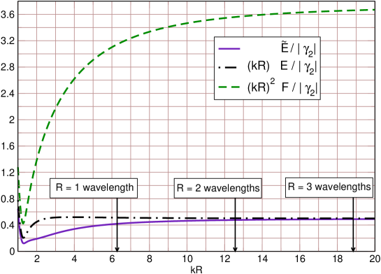
Figure 1: Comparison of the functions $\tilde{E}(kR)$, $E(kR)$, and $F(kR)$ (which are the reflection coefficients times $R/(2M)$ for the boundary conditions $\tilde{\cal B}_{2}$, ${\cal B}_{2}$, and ${\cal C}_{2}$) divided by the reflection coefficient $|\gamma_{2}(kR)|$ for the freezing-$\Psi_{0}$ boundary condition ${\cal B}_{1}$, versus $kR$. Notice that the reflection coefficients are scaled by factors of $kR$ for the sake of the presentation.

For comparison purposes, we plot the function $\tilde{E}(z)/|\gamma_{2}(z)|$ in Figure 1, where the function $\tilde{E}(z)$ was computed in [18] and represents the reflection coefficient resulting from the boundary condition $\tilde{\cal B}_{2}:\left.\partial_{t}(\partial_{t}+\partial_{r})(r^{5}\Psi_{0})\right|_{r=R}=0$ (the same as ${\cal B}_{2}$ but with $\partial_{r_{*}}$ replaced by $\partial_{r}$). We have checked that – as with the functions $E(z)$ and $F(z)$ – the function $\tilde{E}(z)$ is exactly the same in the odd- and the even-parity sector.

IV.2 New boundary conditions which reduce spurious reflections due to the backscattering

Here, we show how to obtain even better boundary conditions: ones which are perfectly absorbing up to order $2M/R$ including the backscatter for quadrupolar gravitational waves. In other words, we now construct boundary conditions which have the property of giving a reflection coefficient that is of the order of $(2M/R)^{2}$ for quadrupolar radiation.

First, by comparing Eq. (36) with $\psi_{0\nearrow}(t,r)=3r^{-4}\left[U(r_{*}-t)+O(2M/R)\right]$, we notice that the boundary condition

$$\left.r(\partial_{t}+\partial_{r_{*}})(r^{5}N^{-1}\Psi_{0})\right|_{r=R}+\frac{30M}{R}\int\limits_{0}^{\infty}\frac{R^{5}\Psi_{0}(t-2Ry,R,\vartheta,\varphi)dy}{(1+y)^{7}}=0$$ (37)

is satisfied up to first order in $2M/R$ for the outgoing solution, the integral operator taking care of the leading order corrections in the backscatter. However, a problem with the boundary condition in Eq. (37) is that it requires knowledge of $\Psi_{0}$ on the whole past portion of the boundary surface. So for a Cauchy formulation which starts an evolution from initial data at the time slice $t=0$, say, this boundary condition is impractical. In order to fix this problem, we split the integral in the expression (36) into two parts:

$$\int\limits_{0}^{\infty}\frac{U(R_{*}-t+2Ry)dy}{(1+y)^{7}}=\int\limits_{0}^{t/2R}\frac{U(R_{*}-(t-2Ry))dy}{(1+y)^{7}}+\int\limits_{t/2R}^{\infty}\frac{U(R_{*}+2Ry-t)dy}{(1+y)^{7}}\;.$$

For a fixed event $(t,R)$ with $t\geq 0$, $R\gg 2M$, the first integral on the right-hand side can be interpreted as an integral over the past line $(\tau,R)$, $0\leq\tau\leq t$, whereas the second integral can be interpreted as an integral over the line $(0,r)$, $R\leq r<\infty$. With this in mind, we replace the boundary condition (37) with the condition:

$$\left.r(\partial_{t}+\partial_{r_{*}})(r^{5}N^{-1}\Psi_{0})\right|_{r=R}+\frac{30M}{R}\int\limits_{0}^{t/2R}\frac{R^{5}\Psi_{0}(t-2Ry,R,\vartheta,\varphi)dy}{(1+y)^{7}}=-\frac{30M}{R}\int\limits_{t/2R}^{\infty}\left.\frac{s^{5}\Psi_{0}(0,s,\vartheta,\varphi)}{(1+y)^{7}}\right|_{s=(R_{*}+2Ry-t)_{\bullet}}dy,$$ (38)

where $(.)_{\bullet}:(-\infty,\infty)\to(2M,\infty)$ denotes the inverse of the transformation $(.)_{*}:(2M,\infty)\to(-\infty,\infty)$ which maps $r$ to $r_{*}$. In particular, $(r_{\bullet})_{*}=r$ and $(r_{*})_{\bullet}=r$. Now the integral on the left-hand side of Eq. (38) only involves the past portion $(\tau,R)$, $0\leq\tau\leq t$, of the boundary point $(t,R)$. The past portion $(\tau,R)$, $\tau<0$, which is not available in a Cauchy evolution starting at $t=0$, is replaced by an integral over the exterior $r>R$ of the initial data. If the initial data are compactly supported in the interval $(0,R)$, this integral is zero and can be discarded. If the initial data do not vanish for $r>R$, one uses the exterior part of the initial data in order to define the integral on the right-hand side of Eq. (38), which acts as a source term in the new boundary condition. The generalization of Eq. (38) to non-spherical boundaries yields the boundary condition ${\cal D}_{2}$ given in Eq. (4).

Summarizing, we have constructed a new boundary condition which is perfectly absorbing up to order $2M/R$ in the backscatter for quadrupolar gravitational radiation. In the appendix, we show for a related model problem that this boundary condition is stable in the sense that it admits an energy estimate.

V Conclusions

In this article, we have analyzed the problem of specifying absorbing outer boundary conditions in general relativity. To this end, we have constructed approximate solutions to the Einstein equations linearized about a Schwarzschild metric of mass $M$ (where $M$ describes the ADM mass of the total spacetime), using the generalized Regge-Wheeler-Zerilli formalism of Ref. [23]. These solutions represent in- and outgoing gravitational radiation in the asymptotic regime $2M/r\ll 1$, where $r$ denotes the areal radius. Since far enough from the strong field region, any stationary asymptotically flat spacetime looks like a Schwarzschild spacetime of mass $M$, these solutions describe, up to order $2M/r$, in- and outgoing gravitational radiation propagating on the asymptotic region of any such spacetime background.

There is an interesting difference between the propagation of even and odd-parity outgoing gravitational linearized radiation on a Schwarzschild background. This difference can be obtained by computing the scalars $\psi_{0}^{(\pm)}$ and $\psi_{4}^{(\pm)}$ on $\tilde{\cal M}$ in the decomposition

$$l^{a}l^{b}V_{abCD} = r\psi_{0}^{(+)}\left[\hat{\nabla}_{C}\hat{\nabla}_{D}\right]^{tf}Y-r\psi_{0}^{(-)}\hat{\nabla}_{(C}\hat{S}_{D)}\;,$$

$$k^{a}k^{b}V_{abCD} = r\psi_{4}^{(+)}\left[\hat{\nabla}_{C}\hat{\nabla}_{D}\right]^{tf}Y+r\psi_{4}^{(-)}\hat{\nabla}_{(C}\hat{S}_{D)}\;$$

of the gauge-invariant quantity $V_{abCD}$ defined in Eq. (16) (recall that $(+)$ refers to even and $(-)$ to odd parity). Using Eqs. (31), (23), and the identity $2r^{3}k^{a}k^{b}\tilde{\nabla}_{a}\tilde{\nabla}_{b}(r\Phi)=N[r^{2}N^{-1}(\partial_{t}-\partial_{r_{*}})]^{2}\Phi$, we obtain the following expressions for the outgoing solution:

$$\psi^{(\pm)}_{0\nearrow}(t,r) = \frac{3}{r^{4}N}\left\{U_{\pm}(r_{*}-t)+\frac{2M}{r}\left[-2U_{\pm}(r_{*}-t)\mp\frac{r}{4}U_{\pm}^{(1)}(r_{*}-t)+\frac{1}{2}\int\limits_{0}^{\infty}k(1+y)U_{\pm}(r_{*}-t+2ry)dy\right]\right.$$ (39)

$$+ \left.O\left(\frac{2M}{R}\right)^{2}\right\},$$

$$\psi^{(\pm)}_{4\nearrow}(t,r) = \frac{3}{r^{4}N}\left\{U_{\pm}(r_{*}-t)-2rU_{\pm}^{(1)}(r_{*}-t)+2r^{2}U_{\pm}^{(2)}(r_{*}-t)-\frac{4}{3}r^{3}U_{\pm}^{(3)}(r_{*}-t)+\frac{2}{3}r^{4}U_{\pm}^{(4)}(r_{*}-t)\right.$$ (40)

$$+ \left.\frac{2M}{r}\left[\frac{1}{2}r^{2}U_{\pm}^{(2)}(r_{*}-t)-\frac{1}{2}r^{3}U_{\pm}^{(3)}(r_{*}-t)+\frac{1}{2}\int\limits_{0}^{\infty}\frac{U_{\pm}(r_{*}-t+2ry)dy}{(1+y)^{2}}\right]+O\left(\frac{2M}{R}\right)^{2}\right\},$$

with $N=1-2M/r$ and $k(w)\equiv 5w^{-6}+4w^{-5}+3w^{-4}+2w^{-3}+w^{-2}$. Taking into account the different normalization of the null tetrad vectors $l^{a}$ and $k^{a}$, and identifying $G(u)=12[U_{+}(r_{*}-t)+iU_{-}(r_{*}-t)]$ with $u=t-r_{*}$, expression (40) agrees precisely with the expression given in Eq. (4.26) of Ref. [25], up to order $M/R$. However, the identification in Ref. [25] of $G(u)$ in Eq. (4.18) with $G(u)$ in Eq. (4.26) is incorrect. Expression (39) agrees with the one given in Eq. (4.18) of Ref. [25] with the identification $G(u)=3[U_{+}(r_{*}-t)+iU_{-}(r_{*}-t)]-3M[U^{(1)}_{+}(r_{*}-t)-iU^{(1)}_{-}(r_{*}-t)]/2$. While the expressions for $\psi^{(\pm)}_{4\nearrow}$ are exactly the same in the odd and even parity sectors, those for the quantity $\psi^{(\pm)}_{0\nearrow}$ differ by a sign in the third term. For $M=0$, there is no difference: even- and odd-parity waves behave in exactly the same way. But as soon as the curvature of the background is taken into account, there is a symmetry breaking between the two parity sectors. Provided sufficient accuracy is available, one should be able to detect this difference in actual numerical simulations.

Using the ingoing and outgoing solutions, and the assumption that the outer boundary is an approximate metric sphere of constant area, we have computed the reflection coefficient which quantifies the amount of spurious radiation reflected into the computational domain by our boundary condition ${\cal B}_{2}$ given in Eq. (2). While this boundary condition is perfectly absorbing for linearized quadrupolar waves, there are small spurious reflections when the curvature of the background is taken into account. However, we have shown that the reflection coefficient due to this effect is extremely small; it is about a factor $M/(kR^{2})$ smaller than the corresponding reflection coefficient for the freezing $\Psi_{0}$ boundary condition which was already found to be small in [18]. By slightly modifying ${\cal B}_{2}$, we obtain a new boundary condition ${\cal C}_{2}$ which results in even less reflections. To give a specific example, if the outer boundary is spherical with areal radius $R>100M$ and quadrupolar waves with wavelength $50M$ are considered, the freezing $\Psi_{0}$ boundary condition yields a reflection coefficient which is smaller than $6.5\times 10^{-5}$. If the boundary condition ${\cal C}_{2}$ is used instead, the reflection coefficient is smaller than $3.1\times 10^{-8}$. Finally, we have found a boundary condition ${\cal D}_{2}$ which takes into account the leading order behavior of the backscatter and is perfectly absorbing up to order $2M/R$ for quadrupolar gravitational radiation. However, this boundary condition is non-local: it involves two integral operators. The first operator involves an integral over the past of the boundary point, the second an integral over the exterior portion of the initial data. It is shown in the appendix for a related model problem that such non-local boundary conditions are stable in that that they admit an energy estimate.

Although our reflection coefficient calculations assume a spherical outer boundary, the formulation of our boundary conditions do not: all that is needed for their construction is that spacetime in the vicinity of the outer boundary can be represented as the product of a two-manifold $\tilde{\cal M}$ and a two-sphere $S^{2}$ such that the assumptions (1) hold.

We have constructed the boundary conditions ${\cal C}_{2}$ and ${\cal D}_{2}$ to reduce spurious reflections for quadrupolar waves. However, in many physically interesting scenarios such as the binary black hole problem, it is possible that when implementing ${\cal D}_{2}$, spurious reflections from the $\ell=3$ octupolar contribution to the gravitational radiation could be as large or larger than the $\ell=2$ quadrupolar backscatter correction. Bardeen [24] has generalized ${\cal C}_{2}$ using the results in [25] to give ${\cal C}_{L}$, a hierarchy of local boundary conditions which is perfectly absorbing including curvature corrections (but neglecting backscatter) to order $2M/R$ for all multipoles of gravitational radiation up to a given angular momentum number $L$. He obtains

$${\cal C}_{L}:~{}~{}~{}~{}~{}\left.\partial_{t}~{}[r^{2}N^{-1}(\partial_{t}+\partial_{r_{*}})]^{L-1}\left(r^{5}N^{-1}\Psi_{0}\right)\right|_{\partial\Sigma}=0.$$ (41)

To determine whether ${\cal C}_{3}$ or ${\cal D}_{2}$ would more effectively reduce spurious reflections when octupolar contributions are taken into account, we have calculated the reflection coefficient due to backscatter of quadrupolar waves for ${\cal C}_{3}$:

$$\Big{|}\gamma\left(kR,\frac{2M}{R}\right)\Big{|}=\frac{45}{4(kR)^{5}}\frac{M}{R}\left[\frac{\left(6C_{7}(kR)-7C_{8}(kR)\right)^{2}+\left(6S_{7}(kR)-7S_{8}(kR)\right)^{2}}{(kR)^{2}+9}\right]^{1/2}+O\left(\frac{2M}{R}\right)^{2}.$$ (42)

Using the asymptotic expansions of $C_{n}(z)$ and $S_{n}(z)$ given in Sect. IV.1, we find that Eq. (42) decays as $(2M/R)(kR)^{-7}$ as $kR\to\infty$. Although not calculated, the reflection coefficient due to backscatter of octupolar waves for ${\cal C}_{3}$ is expected to decay at least as fast or faster. For the boundary condition ${\cal D}_{2}$, we find that when octupolar radiation is considered, the reflection coefficient is (to leading order in $2M/R$) the same as that given in Eq. (96) of [18] and falls off as $(kR)^{-6}$ for large $kR$. We conclude that indeed ${\cal C}_{3}$ would be more effective than ${\cal D}_{2}$ unless the octupolar contributions of the gravitational radiation are significantly suppressed. Using the results in [25], the backscatter corrections to first order in $2M/R$ can in principle be calculated to give ${\cal D}_{3}$ and even ${\cal D}_{L}$.

When applied to full nonlinear formulations of Einstein’s field equations, the boundary conditions ${\cal C}_{L}$ and ${\cal D}_{2}$ on $\Psi_{0}$ should be used along with constraint-preserving boundary conditions and boundary conditions on the gauge degrees of freedom so that the resulting initial-boundary value problem is well posed. A possible strategy for specifying boundary conditions on the gauge degrees of freedom is to insure that the outer boundary is a metric sphere throughout the evolution. This should yield a natural split of the spacetime manifold into a two-dimensional manifold $\tilde{\cal M}$ and the two-sphere $S^{2}$. If the outer boundary is not a metric sphere, our boundary conditions can still be applied; however, the above split of the manifold first needs to be identified. Well posed initial-boundary value formulations incorporating the boundary conditions ${\cal C}_{L}$ and ${\cal D}_{2}$, and their numerical implementation, will be studied in future work.

Appendix A On the stability of non-local boundary conditions

In this appendix, we analyze the following initial-boundary value problem on the quarter space $\Omega_{R}:=(0,\infty)\times(-\infty,R)$, $R>0$:

$$\ddot{u}(t,x)-u^{\prime\prime}(t,x)+V(t,x)u(t,x)=F(t,x), \hbox{$(t,x)\in\Omega_{R}$},$$ (43)

$$\dot{u}(t,R)+u^{\prime}(t,R)+\frac{1}{R^{2}}\int\limits_{0}^{\infty}k_{R}(t,s)u(s,R)ds=G(t), t>0$$ (44)

$$u(0,x)=f(x),\qquad\dot{u}(0,x)=g(x), \hbox{$x<R$}.$$ (45)

Here, a dot and a prime denote differentiation with respect to $t$ and $x$, respectively, $F$ is a given smooth source function on $\Omega_{R}$, $G$ is a given smooth source function on $(0,\infty)$ and $f$ and $g$ are smooth initial data on $(-\infty,R)$. Furthermore, we assume that the potential $V$ in Eq. (43) and the integral kernel $k_{R}(.,.):(0,\infty)^{2}\to\mathbb{R}$ in Eq. (44) satisfy the following three conditions:

1. $V:\Omega_{R}\to\mathbb{R}$ is measurable and bounded in the following sense: There exists a smooth and bounded function $W:(-\infty,R)\to\mathbb{R}$ and a strictly positive constant $p>0$ such that $p/R^{2}\leq W(x)$ for all $x<R$, $V(t,x)\leq W(x)$ for all $(t,x)\in\Omega_{R}$ and

   $$D:=\sup\limits_{(t,x)\in\Omega_{R}}\frac{R^{2}}{\sqrt{p}}\left[W(x)-V(t,x)\right]<\infty.$$

   (If $V$ is smooth, bounded, does not depend on $t$ and satisfies $V(x)\geq p/R^{2}$ for all $x<R$ we can take $W(x)=V(x)$ and $D=0$.)

2. $k_{R}$ satisfies the causality condition $k_{R}(t,s)=0$ if $s>t$,

3. There is a constant $C>0$ which is independent of $R$ such that

   $$\int\limits_{0}^{\infty}|k_{R}(t,s)|dt\leq CR \hbox{for all $s>0$},$$

   $$\int\limits_{0}^{\infty}|k_{R}(t,s)|ds\leq CR \hbox{for all $t>0$}.$$

By a suitable re-definition of $u$ and $F$, if necessary, we can assume that the boundary condition is homogeneous, that is, $G\equiv 0$. In this case, and under the assumptions (i),(ii) and (iii) above, we now show that a sufficiently smooth solution of the IBVP (43,44,45) which vanishes for $x$ sufficiently negative fulfills the energy estimate

$${\cal E}(t)\leq e^{\mu t/R}\left[{\cal E}(0)+aR\int\limits_{0}^{t}\int\limits_{-\infty}^{R}|F(s,r)|^{2}drds\right],$$ (46)

where the energy is defined by

$${\cal E}(t)=\frac{1}{2}\int\limits_{-\infty}^{R}\left(|\dot{u}(t,x)|^{2}+|u^{\prime}(t,x)|^{2}+W(x)|u(t,x)|^{2}\right)dx,$$

and where the dimensionless constants $a$ and $\mu$ are given by

$$a=\frac{1}{2\delta}\,,\qquad\mu=\delta+D+\frac{C^{2}}{2\sqrt{p}}\,,$$

$\delta$ being a strictly positive but otherwise arbitrary constant. The estimate (46) proves uniqueness and continuous dependence of the solution on the data. We do not prove existence of solutions here.

In order to prove the estimate (46) we first differentiate ${\cal E}(t)$ with respect to $t$ and use the evolution equation (43) and assumption (i) and obtain

$$\frac{d}{dt}{\cal E}(t) = \int\limits_{-\infty}^{R}\left\{\dot{u}(t,x)u^{\prime\prime}(t,x)+\dot{u}^{\prime}(t,x)u^{\prime}(t,x)+\left[W(x)-V(t,x)\right]\dot{u}(t,x)u(t,x)+\dot{u}(t,x)F(t,x)\right\}dx$$

$$\leq \dot{u}(t,R)u^{\prime}(t,R)+\frac{D+\delta}{R}{\cal E}(t)+\frac{R}{2\delta}\int\limits_{-\infty}^{R}|F(t,x)|^{2}dx,$$

where $\delta>0$ and where we have used Schwarz’s inequality in the last step. Integrating over $t$ and using the boundary condition (44), we obtain

$${\cal E}(t)-{\cal E}(0) \leq -\int\limits_{0}^{t}|u^{\prime}(s,R)|^{2}ds-\frac{1}{R^{2}}\int\limits_{0}^{t}\int\limits_{0}^{\infty}k_{R}(s,\tau)u^{\prime}(s,R)u(\tau,R)d\tau ds$$ (47)

$$+ \frac{D+\delta}{R}\int\limits_{0}^{t}{\cal E}(s)ds+\frac{R}{2\delta}\int\limits_{0}^{t}\int\limits_{-\infty}^{R}|F(s,x)|^{2}dxds.$$

In order to estimate the second term on the right-hand side, we use assumption (iii) and Schwarz’s inequality again, and obtain

$$\left|\int\limits_{0}^{t}\int\limits_{0}^{\infty}k_{R}(s,\tau)u^{\prime}(s,R)u(\tau,R)d\tau ds\right| \leq \int\limits_{0}^{t}|u^{\prime}(s,R)|\left(\int\limits_{0}^{\infty}|k_{R}(s,\tau)|^{1/2}|k_{R}(s,\tau)|^{1/2}|u(\tau,R)|d\tau\right)ds$$

$$\leq \int\limits_{0}^{t}|u^{\prime}(s,R)|\left(\int\limits_{0}^{\infty}|k_{R}(s,\tau)|d\tau\right)^{1/2}\left(\int\limits_{0}^{\infty}|k_{R}(s,\tau)||u(\tau,R)|^{2}d\tau\right)^{1/2}ds$$

$$\leq (CR)^{1/2}\left(\int\limits_{0}^{t}|u^{\prime}(s,R)|^{2}ds\right)^{1/2}\left(\int\limits_{0}^{t}\int\limits_{0}^{\infty}|k_{R}(s,\tau)||u(\tau,R)|^{2}d\tau ds\right)^{1/2}.$$

Using Fubini’s theorem, the causality condition (ii) and condition (iii), we have

$$\int\limits_{0}^{t}\int\limits_{0}^{\infty}|k_{R}(s,\tau)||u(\tau,R)|^{2}d\tau ds=\int\limits_{0}^{\infty}\int\limits_{0}^{t}|k_{R}(s,\tau)|ds|u(\tau,R)|^{2}d\tau=\int\limits_{0}^{t}\int\limits_{0}^{t}|k_{R}(s,\tau)|ds|u(\tau,R)|^{2}d\tau\leq CR\int\limits_{0}^{t}|u(\tau,R)|^{2}d\tau.$$

Therefore,

$$\left|\int\limits_{0}^{t}\int\limits_{0}^{\infty}k_{R}(s,\tau)u^{\prime}(s,R)u(\tau,R)d\tau ds\right|\leq CR\left(\int\limits_{0}^{t}|u^{\prime}(s,R)|^{2}ds\right)^{1/2}\left(\int\limits_{0}^{t}|u(s,R)|^{2}ds\right)^{1/2}.$$ (48)

The estimates (47,48) imply that

$${\cal E}(t)-{\cal E}(0) \leq -\left[\left(\int\limits_{0}^{t}|u^{\prime}(s,R)|^{2}ds\right)^{1/2}-\frac{C}{2R}\left(\int\limits_{0}^{t}|u(s,R)|^{2}ds\right)^{1/2}\right]^{2}$$

$$+ \frac{C^{2}}{4R^{2}}\int\limits_{0}^{t}|u(s,R)|^{2}ds+\frac{D+\delta}{R}\int\limits_{0}^{t}{\cal E}(s)ds+\frac{R}{2\delta}\int\limits_{0}^{t}\int\limits_{-\infty}^{R}|F(s,x)|^{2}dxds$$

$$\leq \frac{C^{2}}{4R^{2}}\int\limits_{0}^{t}|u(s,R)|^{2}ds+\frac{D+\delta}{R}\int\limits_{0}^{t}{\cal E}(s)ds+\frac{R}{2\delta}\int\limits_{0}^{t}\int\limits_{-\infty}^{R}|F(s,x)|^{2}dxds.$$

Finally, using the Sobolev type estimate

$$|u(s,R)|^{2}=\int\limits_{-\infty}^{R}\partial_{x}[u(s,x)^{2}]dx=2\int\limits_{-\infty}^{R}u(s,x)u^{\prime}(s,x)dx\leq\frac{2R}{\sqrt{p}}\,{\cal E}(s),$$

we obtain the estimate (46) after the application of Gronwall’s lemma.

As an application of our result, consider the massless scalar wave equation on a Schwarzschild background of mass $M$. Performing a decomposition of the scalar field $\Phi$ into spherical harmonics $Y^{\ell m}$,

$$\Phi(t,r,\vartheta,\varphi)=\frac{1}{r}\sum\limits_{\ell=0}^{\infty}\sum\limits_{m=-\ell}^{\ell}\phi_{\ell m}(t,r)Y^{\ell m}(\vartheta,\varphi),$$

the wave equation reads

$$\left[\partial_{t}^{2}-\partial_{r_{*}}^{2}+\left(1-\frac{2M}{r}\right)\left(\frac{\ell(\ell+1)}{r^{2}}+\frac{2M}{r^{3}}\right)\right]\phi_{\ell m}=0,$$ (49)

In outgoing Eddington-Finkelstein coordinates $\tau=t+r-r_{*}$, $\rho=r$, this equation assumes the form

$$\left[\partial_{\tau}^{2}-\partial_{\rho}^{2}+\frac{\ell(\ell+1)}{\rho^{2}}\right]\phi_{\ell m}=-\frac{2M}{\rho}\left[(\partial_{\tau}+\partial_{\rho})^{2}-\frac{1}{\rho}(\partial_{\tau}+\partial_{\rho})+\frac{1}{\rho^{2}}\right]\phi_{\ell m}\,.$$

Monopolar outgoing solutions have the form (omitting the indices $00$ on $\phi$)

$$\phi(t,r)=U(r_{*}-t)+2M\int\limits_{r_{*}-t}^{\infty}\frac{U(x)dx}{(t+2r-r_{*}+x)^{2}}+O\left(\frac{2M}{R}\right)^{2},$$

where $U$ is a smooth and bounded function which vanishes if its argument is sufficiently negative. Since

$$(\partial_{t}+\partial_{r_{*}})\phi(t,r)=-\frac{2M}{r^{2}}\int\limits_{0}^{\infty}\frac{U(r_{*}-t+2ry)dy}{(1+y)^{3}}+O\left(\frac{2M}{R}\right)^{2},$$

the boundary condition

$$(\partial_{t}+\partial_{r_{*}})\phi(t,R)+\frac{2M}{R^{2}}\int\limits_{0}^{t/2R}\frac{\phi(t-2Ry,R)dy}{(1+y)^{3}}=G(t),$$ (50)

where

$$G(t)=-\frac{2M}{R^{2}}\int\limits_{t/2R}^{\infty}\frac{\phi(0,(R_{*}+2Ry-t)_{\bullet},R)dy}{(1+y)^{3}}\;,$$

is perfectly absorbing up to order $2M/R$. Performing the substitutions $x=r_{*}$ and $y=(t-s)/2R$ equation (49) can be brought into the form (43) and the boundary condition (50) into the form (44), where

$$k_{R}(t,s)=\left\{\begin{array}[]{ll}\frac{M}{R}\frac{(2R)^{3}}{(2R+t-s)^{3}}\,,&0\leq s\leq t,\\ 0,&s>t.\end{array}\right.$$

This kernel satisfies the assumptions (ii) and (iii) with $C=M/R$, and the potential in Eq. (49) is smooth, positive and bounded by the constant $W:=[\ell(\ell+1)+1]/(2M)^{2}$; hence, it satisfies assumption (i). For linear fluctuations of a Schwarzschild background, Eq. (49) has to be replaced by the Regge-Wheeler or Zerilli equation (21), and our boundary condition ${\cal D}_{2}$ involves third derivatives of the fields. Therefore, it is not of the form (44). However, it can be reduced to a first order system for which an energy estimate similar to the one presented above can be found by introducing auxiliary variables as in the method used in the appendix of Ref. [18].

References

- [1] H. Friedrich and G. Nagy. The initial boundary value problem for Einstein’s vacuum field equations. Comm. Math. Phys., 201:619–655, 1999.
- [2] L.E. Kidder, L. Lindblom, M.A. Scheel, L.T. Buchman, and H.P. Pfeiffer. Boundary conditions for the Einstein evolution system. Phys. Rev. D, 71:064020(1)–064020(22), 2005.
- [3] O. Sarbach and M. Tiglio. Boundary conditions for Einstein’s field equations: Mathematical and numerical analysis. Journal of Hyperbolic Differential Equations, 2:839–883, 2005.
- [4] L. Lindblom, M.A. Scheel, L.E. Kidder, R. Owen, and O. Rinne. A new generalized harmonic evolution system. Class. Quantum Grav., 23:S447–S462, 2006.
- [5] O. Rinne. Stable radiation-controlling boundary conditions for the generalized harmonic Einstein equations. Class. Quantum Grav., 23:6275–6300, 2006.
- [6] G. Nagy and O. Sarbach. A minimization problem for the lapse and the initial-boundary value problem for Einstein’s field equations. Class. Quantum Grav., 23:S477–S504, 2006.
- [7] M.C. Babiuc, B. Szilagyi, and J. Winicour. Harmonic initial-boundary evolution in general relativity. Phys. Rev. D, 73:064017(1)–064017(23), 2006.
- [8] H.O. Kreiss and J. Winicour. Problems which are well-posed in a generalized sense with applications to the Einstein equations. Class. Quantum Grav., 23:S405–S420, 2006.
- [9] M.C. Babiuc, H-O. Kreiss, and J. Winicour. Constraint-preserving Sommerfeld conditions for the harmonic Einstein equations. Phys. Rev. D, 75:044002(1)–044002(13), 2007.
- [10] B. Zink, E. Pazos, P. Diener, and M. Tiglio. Cauchy-perturbative matching revisited: Tests in spherical symmetry. Phys. Rev. D, 73:084011(1)–084011(14), 2006.
- [11] J. Novak and S. Bonazzola. Absorbing boundary conditions for simulation of gravitational waves with spectral methods in spherical coordinates. J. Comp. Phys., 197:186–196, 2004.
- [12] S. Bonazzola, E. Gourgoulhon, P. Grandcl\a’ement, and J. Novak. Constrained scheme for the Einstein equations based on the Dirac gauge and spherical coordinates. Phys. Rev. D, 70:104007(1)–104007(24), 2004.
- [13] M. Choptuik, L. Lehner, I. Olabarrieta, R. Petryk, F. Pretorius, and H. Villegas. Towards the final fate of an unstable black string. Phys. Rev. D, 68:044001(1)–044001(11), 2003.
- [14] F. Pretorius. Evolution of binary black-hole spacetimes. Phys. Rev. Lett., 95:121101(1)–121101(4), 2005.
- [15] H. Friedrich. On the regular and asymptotic characteristic initial value problem for Einstein’s vacuum field equations. Proc. R. Soc. Lond. A, 375:169–184, 1981.
- [16] J. Frauendiener. Numerical treatment of the hyperboloidal initial value problem for the vacuum Einstein equations. 2. the evolution equations. Phys. Rev. D, 58:064003(1)–064003(18), 1998.
- [17] S. Husa, C. Schneemann, T. Vogel, and A. Zenginoğlu. Hyperboloidal data and evolution. AIP Conf. Proc., 841:306–313, 2006.
- [18] L.T. Buchman and O.C.A. Sarbach. Towards absorbing outer boundaries in general relativity. Class. Quantum Grav., 23:6709–6744, 2006.
- [19] S.R. Lau. Rapid evaluation of radiation boundary kernels for time-domain wave propagation on blackholes: theory and numerical methods. J. Comput. Phys., 199:376–422, 2004.
- [20] S.R. Lau. Rapid evaluation of radiation boundary kernels for time-domain wave propagation on black holes: implementation and numerical tests. Class. Quantum Grav., 21:4147–4192, 2004.
- [21] S.R. Lau. Analytic structure of radiation boundary kernels for blackhole perturbations. J. Math. Phys., 46:102503(1)–102503(21), 2005.
- [22] E. Pazos, E.N. Dorband, A. Nagar, C. Palenzuela, E. Schnetter, and M. Tiglio. How far away is far enough for extracting numerical waveforms, and how much do they depend on the extraction method?, 2006. gr-qc/0612149.
- [23] O. Sarbach and M. Tiglio. Gauge invariant perturbations of Schwarzschild black holes in horizon penetrating coordinates. Phys. Rev. D, 64:084016(1)–(15), 2001.
- [24] J.M. Bardeen, 2007. Private communication.
- [25] J.M. Bardeen and W.H. Press. Radiation fields in the Schwarzschild background. J. Math. Phys., 14:7–19, 1973.
- [26] T. Regge and J. Wheeler. Stability of a Schwarzschild singularity. Phys. Rev., 108:1063–1069, 1957.
- [27] F. Zerilli. Effective potential for even-parity Regge-Wheeler gravitational perturbation equations. Phys. Rev. Lett., 24:737–738, 1970.
- [28] S.A. Teukolsky. Perturbations of a rotating black hole. 1. fundamental equations for gravitational electromagnetic, and neutrino field perturbations. Astrophys. J., 185:635–647, 1973.
- [29] U.H. Gerlach and U.K. Sengupta. Gauge-invariant perturbations on most general spherically symmetric space-times. Phys. Rev. D, 19:2268–2272, 1979.
- [30] R.H. Price. Nonspherical perturbations of relativistic gravitational collapse. II. Integer-spin, zero-rest-mass fields. Phys. Rev. D, 5:2439–2454, 1972.
- [31] R. Penrose. Zero rest-mass fields including gravitation: asymptotic behaviour. Proc. R. Soc. Lond. A, 284:159–203, 1965.
- [32] S. Chandrasekhar. The Mathematical Theory of Black Holes. Oxford University Press, Great Clarendon Street, Oxford 0X2 6DP, 1992.