Luminosity distance-redshift relation for the LTB solution near the center

1 Introduction

Modern observations show that the Universe is presently in an accelerating phase and dominated by dark energy with negative pressure [1, 2, 3, 4, 5]. It is remarkable that there seems no obvious contradiction among the observations, but the true nature of dark energy is a great mystery. On the other hand, it is also true that this recognition is a result of the strict use of a Friedmann-Lemaître-Robertson-Walker (FLRW) homogeneous and isotropic model. If inhomogeneities are properly taken into account it might be possible to explain the observations without introducing dark energy. Recently, this possibility has renewed interest in inhomogeneous cosmological models, especially in the so-called Lemaître-Tolman-Bondi (LTB) solution [6, 7, 8], which represents a spherically symmetric dust-filled universe. Because of its simplicity this solution has been considered to be most useful to evaluate the effect of inhomogeneities in the observables like the luminosity distance-redshift relation.

Although this solution is simple, it has great flexibility. Various models have been proposed that are consistent with the observations [9, 10, 11, 12, 13, 14, 15]. But, what is the best configuration that can explain the observations of, e.g., luminosity distance redshift relation for type Ia supernovae and still be consistent with other observations? To respond to this question one needs a systematic approach.

Our primary focus is the “inverse problem” approach, in which one takes a luminosity distance function $D_{L}(z)$ as an input to select a specific LTB model. Mustapha et.al. [16] argued that the free functions in the LTB solution can be chosen to match any given luminosity distance function $D_{L}(z)$ and source evolution function $m(z)$. Célérier [9] performed an expansion of $D_{L}(z)$ for the LTB solution of parabolic type to fit the $\Lambda$CDM model with $\Omega_{\Lambda}=0.7$ and $\Omega_{M}=0.3$, and argued that the model can explain the SNIa observation at least for $z\lesssim 1$. Vanderveld et.al. [17] however showed that such a fitting with an accelerating model is only possible at the cost of occurrence of weak singularity at the center.

The main purpose of this paper is to find a Taylor expansion of $D_{L}(z)$ for the LTB solution in the most general form, not restricted to the parabolic type, with considerations for the condition to avoid the weak singularity. Since the differential equation for the inverse problem is in general singular at the origin $z=0$ it is imperative to prepare a solution there using a different method. If we have the expansion of $D_{L}(z)$ for the general LTB solution, we can easily find this solution by comparing the given $D_{L}(z)$ and that of the LTB solution order by order.

To perform the computation we present a new way of representing the LTB solution. Although this is not our main purpose we would like to stress that this new representation would be very useful in various computations concerning the LTB solution. This solution is usually expressed with parametric functions, as is the FLRW dust solution. This parametric character of the solution often makes our analysis and considerations complicated and non-transparent. Moreover those functions change their forms depending on whether the solution is of spherical type, parabolic type, or hyperbolic type. This split-into-cases character is also a drawback of the conventional expression of the solution. The new expression of the solution dissolves all these unwanted characters. It will play an essential role to achieve the complicated computations needed to compute $D_{L}(z)$ in the fully general setting.

The structure of this paper is as follows. In section 2 we introduce the new unified form of the LTB solution. In section 3 we perform the expansion of $D_{L}(z)$ using the unified expression. In section 4 we study how different the function $D_{L}(z)$ for the LTB solution is from that of the FLRW dust solution. Section 5 is devoted to conclusion. Appendix A presents the result without the regularity condition at the center.

2 The LTB solution in a unified new form

Let us first gather the conventional forms of the solution. The LTB metric is written in the form

$$ds^{2}=-dt^{2}+\frac{{R^{\prime}(t,r)}^{2}}{1+2E(r)}dr^{2}+R(t,r)^{2}(d\theta^{2}+\sin^{2}\theta d\phi^{2}),$$ (1)

where primes denote derivatives with respect to the radial coordinate $r$, and $E(r)$ is a free function called the “energy function”. The conventional way of expressing the areal radius function $R(t,r)$ depends on the sign of $E(r)$ and is parametric: For $E(r)>0$, we have

$$R(t,r) =\frac{M(r)}{2E(r)}(\cosh\eta-1),$$ (2)

$$t-t_{B}(r) =\frac{M(r)}{(2E(r))^{3/2}}(\sinh\eta-\eta),$$ (3)

where $M(r)$ and $t_{B}(r)$ are free functions called, respectively, the “mass function” and the “big bang function”. For $E(r)<0$, we have

$$R(t,r) =\frac{M(r)}{-2E(r)}(1-\cos\eta),$$ (4)

$$t-t_{B}(r) =\frac{M(r)}{(-2E(r))^{3/2}}(\eta-\sin\eta).$$ (5)

Finally, for $E(r)=0$, we have

$$R(t,r)=\left(\frac{9}{2}\right)^{1/3}M(r)^{1/3}(t-t_{B}(r))^{2/3}.$$ (6)

(In this case the function $R(t,r)$ is explicit in terms of $t$ and $r$.)

Now, observe that in the $E>0$ case, Eq.(3) shows that $\eta$ can be regarded as a function of $2E((t-t_{B})/M)^{2/3}$. Therefore from Eq.(2) the function $R$ can be written in the form

$$R(t,r)=\frac{M}{2E}X\left(2E\left(\frac{t-t_{B}}{M}\right)^{2/3}\right),$$ (7)

using a certain function $X(x)$. To make the $E\rightarrow 0$ limit apparently regular, we then factor out $x$ from the function $X(x)$ and make $X(x)=6^{1/3}x\mathcal{S}(-6^{-2/3}x)$;

$$R(t,r)=(6M(r))^{1/3}(t-t_{B}(r))^{2/3}\mathcal{S}\left(-2E(r)\left(\frac{t-t_{B}(r)}{6M(r)}\right)^{2/3}\right).$$ (8)

(The numerical factors inserted are our convention.)

The same observation is also applicable to both $E<0$ and $E=0$ cases, and as a result, we find that the form (8) may provide a desirable form of $R(t,r)$, which is explicit in terms of $t$ and $r$ and requires no separate considerations depending on the sign of $E(r)$. There is, however, still a remaining task, which is to confirm that the function $\mathcal{S}(x)$ is smooth at $x=0$. Otherwise, this form would be superficial.

To this, note that the function $\mathcal{S}(x)$ can be expressed in parametric forms. For $x<0$ (corresponding to $E>0$), we have

$$\mathcal{S}(x)={1\over 6^{1/3}}\frac{\cosh\sqrt{-\zeta}-1}{(\sinh\sqrt{-\zeta}-\sqrt{-\zeta})^{2/3}},\quad x=\frac{-1}{6^{2/3}}(\sinh\sqrt{-\zeta}-\sqrt{-\zeta})^{2/3}.$$ (9)

For $x>0$ ($E<0$), we have

$$\mathcal{S}(x)={1\over 6^{1/3}}\frac{1-\cos\sqrt{\zeta}}{(\sqrt{\zeta}-\sin\sqrt{\zeta})^{2/3}},\quad x={1\over 6^{2/3}}(\sqrt{\zeta}-\sin\sqrt{\zeta})^{2/3}.$$ (10)

For $x=0$, we have

$$\mathcal{S}(0)=\left(\frac{3}{4}\right)^{1/3}.$$ (11)

The parameter $\zeta$ takes positive and negative values in accordance with the sign of $x$. (The explicit correspondence to $\eta$ is given by $\zeta=\eta^{2}$ for $E<0$, and $\zeta=-\eta^{2}$ for $E>0$.) We then find that $\mathcal{S}$ and $x$ are expanded in powers of $\zeta$ in the same form for all signs of $x$, since by direct computation we can immediately confirm the following common expression:

$$\mathcal{S}(x)={1\over 6^{1/3}}\frac{\frac{1}{2}-\frac{1}{4!}\zeta+\cdots}{\left(\frac{1}{3!}-\frac{\zeta}{5!}+\cdots\right)^{2/3}},\quad x=\frac{\zeta}{6^{2/3}}\left(\frac{1}{3!}-\frac{\zeta}{5!}+\cdots\right)^{2/3}.$$ (12)

Proceeding the series expansions,

$$\begin{split}\mathcal{S}(x)&=\left(\frac{3}{4}\right)^{1/3}\left(1-\frac{\zeta}{20}+\frac{\zeta^{2}}{1680}+O(\zeta^{3})\right),\\ x&=6^{-4/3}\left(\zeta-\frac{\zeta^{2}}{30}+\frac{13\zeta^{3}}{25200}+O(\zeta^{4})\right).\end{split}$$ (13)

Since both $\mathcal{S}$ and $x$ are smooth (in fact, analytic) functions of $\zeta$, in particular in the neighborhood of $\zeta=0$, this shows that $\mathcal{S}(x)$ is smooth at $x=0$, as desired. (The smoothness of $\mathcal{S}(x)$ at $x\neq 0$ is apparent.) Figure 1 shows a plot of the function $\mathcal{S}(x)$. $\mathcal{S}(x)$ is a non-negative, monotonic function, defined for $x\leq x_{C}\equiv(\pi/3)^{2/3}$.

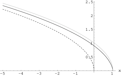
Figure 1: Plots of the function $\mathcal{S}(x)$ (solid line), the function $\mathcal{\tilde{V}}_{0}(x)=\sqrt{-x}$ (dashed line), and the function $\mathcal{S}_{C}(x)=\sqrt{x_{C}-x}$ (gray line). Although the parametric expression of $\mathcal{S}(x)$ takes different forms for $x>0$, $x=0$, and $x<0$, this function is smooth at the dividing point $x=0$.

The expression (8) therefore does provide a desired form of the LTB solution, together with the conventional metric form (1). This expression will turn out to be extremely useful in performing most of the computations concerning the LTB solution, including the expansion of $D_{L}(z)$ in the next section. In the rest of this section we briefly discuss some useful properties concerning the function $\mathcal{S}(x)$.

First, remember that $R(t,r)$ satisfies the following generalized ‘Friedmann’ equation:

$${\dot{R}}^{2}=\frac{2M}{R}+2E,$$ (14)

where dots denote derivatives with respect to the proper time $t$. Substituting Eq.(8) we immediately have the first order ordinary differential equation (ODE) for $\mathcal{S}(x)$:

$$\frac{4}{3}(\mathcal{S}(x)+x\mathcal{S}^{\prime}(x))^{2}+3x-{1\over\mathcal{S}(x)}=0,$$ (15)

where $\mathcal{S}^{\prime}\equiv d\mathcal{S}(x)/dx$. (We understand that primes attached to $\mathcal{S}$ always stand for derivatives with respect to its single argument, not to the radial coordinate $r$).

This ODE has a peculiar feature observed at $x=0$; at this point the term $x\mathcal{S}^{\prime}(x)$ vanishes and therefore the equation degenerates into an algebraic equation that constrains $\mathcal{S}(0)$, provided that $|\mathcal{S}^{\prime}(0)|<\infty$. As a result we obtain $S(0)=(3/4)^{1/3}$ in accordance with Eq.(11). The finiteness condition of $S^{\prime}(x)$ at $x=0$ implies that the line $y=S(x)$ in the $x$-$y$ plane should intersect the $x=0$ axis transversely. The above feature therefore tells us that the function $S(x)$ is the unique ‘transversal’ solution of the ODE (15). It may be useful to use this characterization to define $S(x)$, instead of using the explicit parametric expressions (9), (10), and (11).

It may be worth commenting that we should not think of the ODE (15) as a usual ‘evolution equation,’ because of the following two reasons. First, as discussed previously, this ODE has no freedom to choose an initial value. Note that the solution of the generalized Friedmann equation (14) does possess freedom to choose an initial data, which is the function $t_{B}(r)$. This function is however already incorporated in the form (8). The resulting equation therefore cannnot contain further freedom to choose a solution. Second, the gradient of the variable $x(t,r)$ for the ODE is in general not timelike. In other words, the contours of $x(t,r)$ are not always spacelike. This is most noticeable when $E(r)$ crosses zero at some spatial points. Figure 2 shows an example where $E(r)$ crosses zero at one point ($r=1$).

Figure 2: Typical contours of $x(t,r)$ when $E(r)$ crosses zero. The decreasing bold curve corresponds to the Big Bang singularity ($t=t_{B}(r)$), while the vertical bold line to $E(r)=0$ (this is not a singularity). Both bold lines correspond to $x=0$. Contours are drawn for $t\geq t_{B}(r)$. [This example is intended to be helpful for a general discussion of the properties of $\mathcal{S}(x)$, and not to imply a setting of the next section. The specific choice for this example is $E(r)=-r^{2}(1/2-\theta_{0.4}(r-1))$, $M(r)=r^{3}$, and $t_{B}(r)=e^{-r^{2}}$. The function $\theta_{\sigma}(r)$ is a step function with the transition interval $[-\sigma,\sigma]$ with values $\theta_{\sigma}(r)=1(r\geq\sigma)$, and $0(r\leq-\sigma)$.]

Note that the form (8) already contains the parabolic solution as one factor, with the remaining factor being $S(x)$. We can think of $|x|$ as a parameter that measures the deviation from the parabolic evolution. It is obvious that $x=0$ corresponds to both big bang time $t=t_{B}(r)$ and comoving points $E(r)=0$. In the above example, these two regions are shown as the bold lines forming an inverted ‘T’-shape (Fig.2). Let us consider a neighborhood of this ‘T’-shaped region such that for a small positive $\epsilon$, $|x|<\epsilon$. Then we can say that the time evolution of the points contained in this spacetime region is close to that of the parabolic solution. Actually, for small $t-t_{B}(r)$ this is a well-known fact. (Both elliptic and hyperbolic solutions asymptotically approach the parabolic type evolution $(t-t_{B}(r))^{2/3}$ near the big bang time.) It is also apparent that if $|E(r)|$ is small enough the evolution of those points is close to that of the parabolic solution (for a finite time-interval). The variable $x$ is therefore a deviation parameter, rather than a evolution parameter.

Now, let us return to the discussion of useful properties of $\mathcal{S}(x)$. Remember that Eq.(14) is an integral of the following second order partial differential equation:

$$2R\ddot{R}+\dot{R}^{2}-2E=0.$$ (16)

From this we have the second order ODE for $\mathcal{S}(x)$:

$$x(2\mathcal{S}(x)\mathcal{S}^{\prime\prime}(x)+{\mathcal{S}^{\prime}}^{2}(x))+5\mathcal{S}(x)\mathcal{S}^{\prime}(x)+\frac{9}{4}=0.$$ (17)

For $x\neq 0$, this equation is useful in case we want to eliminate higher derivatives of $\mathcal{S}(x)$ than first order.

When $x=0$, Eq.(17) itself does not determine $\mathcal{S}^{\prime\prime}(0)$, due to the multiplied factor $x$. However, we can regard this equation as an equation that determines $\mathcal{S}^{\prime}(0)$ from $\mathcal{S}(0)$, and find $\mathcal{S}^{\prime}(0)=-9/(20\mathcal{S}(0))$. Similarly, taking derivatives of the equation we can successively determine the values of arbitrarily higher derivatives of $\mathcal{S}(x)$ at $x=0$, in terms of $\mathcal{S}(0)$. One of the useful applications of this property is to obtain a series expansion of $\mathcal{S}(x)$ about $x=0$. Since $\mathcal{S}(0)$ is given in Eq.(11) (or determined from Eq.(15)), we have

$$\mathcal{S}(x)=\left(\frac{3}{4}\right)^{1/3}\left(1-\frac{3}{5}\left(\frac{3}{4}\right)^{1/3}x-\frac{27}{350}\left(\frac{9}{2}\right)^{1/3}x^{2}+O(x^{3})\right).$$ (18)

As discussed previously, this expansion can provide a ‘parabolic approximation’ of the solution.

We may be interested in the significance of the general solutions of the ODE (17). To avoid confusions let us top tilde, like $\tilde{\mathcal{S}}(x)$, to denote a solution of the ODE which does not necessarily coincide with $\mathcal{S}(x)$. First, the above observation immediately tells us that a solution of the ODE which intersects the $x=0$ axis transversely is specified only by one parameter $s\equiv\tilde{\mathcal{S}}(0)$, since ${\tilde{\mathcal{S}}}^{\prime}(x)$ is not free at $x=0$. We can easily confirm that all those transversal solutions are generated from $\mathcal{S}(x)$ by rescaling:

$$\tilde{\mathcal{S}}_{\alpha}(x)=\alpha\mathcal{S}\left(\frac{x}{\alpha^{2}}\right),$$ (19)

where $\alpha=s/\mathcal{S}(0)=(4/3)^{1/3}s$. This rescaled function is also a solution of the first order ODE (15) with the modification $1/\mathcal{S}\rightarrow 1/(\alpha^{3}\mathcal{S})$. These rescaling of the function and modification of the equation just correspond to the rescaling $M(r)\rightarrow\alpha^{3}M(r)$, and therefore although the rescaled function $\tilde{\mathcal{S}}_{\alpha}(x)$ does generate a dust solution, it is equivalent to the one by the original $\mathcal{S}(x)$. Thus, we may not be interested in the general transversal solution $\tilde{\mathcal{S}}_{\alpha}(x)$.

Non-transversal solutions of the ODE (17) in general have two-parameters. An interesting one-parameter special solution is

$$\mathcal{\tilde{V}}_{\beta}(x)=\sqrt{-x}-\frac{\beta}{x},$$ (20)

where $\beta$ is an arbitrary constant parameter. $\mathcal{\tilde{V}}_{\beta}(x)$ approaches $\mathcal{S}(x)$ as $x\rightarrow-\infty$:

$$\mathcal{\tilde{V}}_{\beta}(x)\rightarrow\mathcal{S}(x)\quad(x\rightarrow-\infty).$$ (21)

In particular, $\mathcal{\tilde{V}}_{0}(x)=\sqrt{-x}$ approaches $\mathcal{S}(x)$ from below (Fig.1), and is often useful for various estimates of $\mathcal{S}(x)$ for large $-x$. We remark that the function $\mathcal{\tilde{V}}_{\beta}(x)$ satisfies the first order ODE (15) if the $1/\mathcal{S}(x)$ term in the equation is neglected. This in effect corresponds to taking the limit $M(r)\rightarrow 0$, and therefore the metric generated by this function (through Eq.(8) with $\mathcal{S}(x)$ replaced by $\mathcal{\tilde{V}}_{\beta}(x)$) represents a vacuum solution. In fact, by a direct computation of the Riemann tensor we find that it all represents the Minkowski solution.

Finally, it is worth mentioning that, slightly modifying $\mathcal{\tilde{V}}_{0}(x)$, the function

$$\mathcal{S}_{C}(x)\equiv\sqrt{x_{C}-x},$$ (22)

which is no longer a solution of any of the ODEs, provides a good approximation of $\mathcal{S}(x)$ for all domain of $x\leq x_{C}$. The function $\mathcal{S}_{C}(x)$ asymptotically approaches $\mathcal{S}(x)$ from above as $x\rightarrow-\infty$ (Fig.1). An elementary estimate actually confirms the inequality

$$\mathcal{S}(x)\leq\mathcal{S}_{C}(x),$$ (23)

where the equality holds for $x=x_{C}$. Also, another elementary estimate establishes

$$x\mathcal{S}^{\prime}(x)<\frac{\mathcal{S}(x)}{2}$$ (24)

for the first derivative.

3 Expansion of $D_{L}(z)$

Motivated by the inverse problem, we in this section perform the expansion of the function $D_{L}(z)$, the luminosity distance as a function of the redshift, for the LTB solution.

The luminosity distance for the LTB solution is simply given by [19, 20]

$$D_{L}=(1+z)^{2}R,$$ (25)

where the areal radius function $R=R(t(z),r(z))$ must be evaluated along the light ray emitted from the light source and caught by the central observer at $(t,r)=(t_{0},0)$. With this formula we can expand $D_{L}(z)$ if we expand $R$.

Before proceeding the expansion, we note that the LTB solution has the gauge freedom of choosing the radial coordinate $r$. In fact, it is easy to see that coordinate transformation $r\rightarrow\tilde{r}=\tilde{r}(r)$ retains the characteristic form of the solution if we redefine the free functions $E(r),t_{B}(r)$, and $M(r)$ suitably. The significance of this freedom is that it enables us to fix the function $M(r)$ for many cases.

One of the popular gauge choices is (e.g., [9, 14, 17]) to take $M(r)=M_{0}r^{3}$ with $M_{0}$ being a positive constant. We call this choice the FLRW gauge, since the standard form of the FLRW dust solution is realized with this choice with the other functions being $E(r)=-(k/2)r^{2}$, and $t_{B}(r)=0$. ($k$ is the curvature constant.)

Another excellent choice is [21, 16] to choose the radial coordinate $r$ so that the light rays coming into the observer are simply expressed by

$$t=t_{0}-r.$$ (26)

This is equivalent to the condition that $dr/dt=-1$ must hold along those light rays, and therefore from the metric (1) it is equivalent to imposing

$$\frac{R^{\prime}(t_{0}-r,r)}{\sqrt{1+2E(r)}}=1,$$ (27)

where $R^{\prime}(t_{0}-r,r)\equiv(\partial R(t,r)/\partial r)|_{t=t_{0}-r}$. This gauge choice determines the function $M(r)$ only simultaneously with $E(r)$ and $t_{B}(r)$. We call this choice of $r$ or the resulting choice of $M(r)$ the light cone gauge.

We in the following adopt the light cone gauge, which, together with the formula (8), makes our procedure of expansion systematic and straightforward. In fact, with the condition (26) we can firstly expand $R$ in powers of $r$ in a straightforward manner, putting $R=R(t_{0}-r,r)$ in the formula (8). To convert the result into expansion in terms of $z$, we need to find $r(z)$ in powers of $z$. This is possible from the formula[9]

$$\frac{dr}{dz}=\frac{\sqrt{1+2E(r)}}{(1+z){\dot{R}}^{\prime}(t_{0}-r,r)}.$$ (28)

This would complete our expansion, but we still need to consider an extra condition, which is the regularity at $r=0$. As pointed out in [17, 22], if the first derivative with respect to $r$ of the matter density $\rho(t,r)$ does not vanish at $r=0$, the spacetime has a weak singularity there. We wish to eliminate this undesirable feature; therefore impose

$$\rho^{\prime}(t,0)=0.$$ (29)

The expansion with this condition imposed will give the final form of our result.

We are now in a position to proceed the expansion, following the procedure outlined above. We wish to expand $D_{L}(z)$ up to the third order, which leads us to expand the free functions as follows:

$$\begin{split}E(r)&=\frac{e_{2}}{2}r^{2}+\frac{e_{3}}{3!}r^{3}+\frac{e_{4}}{4!}r^{4}+O(r^{5}),\\ t_{B}(r)&={b_{1}}r+\frac{b_{2}}{2}r^{2}+O(r^{3}),\\ M(r)&=\frac{m_{3}}{3!}r^{3}+\frac{m_{4}}{4!}r^{4}+\frac{m_{5}}{5!}r^{5}+O(r^{6}),\end{split}$$ (30)

where the differential coefficients $e_{i}\equiv E^{(i)}(0)$, $b_{i}\equiv t_{B}^{(i)}(0)$, and $m_{i}\equiv M^{(i)}(0)$ are constants, with $m_{3}>0$. Our task is then to express the expansion of $D_{L}(z)$ in terms of these coefficients.

It turns out to be convenient to, prior to the general computations, finish the computation for the first order of $D_{L}(z)$ to determine the Hubble constant $H_{0}$ in comparison with the definition $D_{L}(z)=z/H_{0}+O(z^{2})$. This is not very much elaborating, and we find

$$H_{0}=\frac{2}{3t_{0}}\left(1+x_{0}\frac{\mathcal{S}^{\prime}(x_{0})}{\mathcal{S}(x_{0})}\right),\quad x_{0}\equiv-e_{2}\left(\frac{t_{0}}{m_{3}}\right)^{2/3}.$$ (31)

(As remarked, prime attached to $\mathcal{S}(x)$ stands for the derivative with respect to $x$, not with respect to $r$; $\mathcal{S}^{\prime}(x_{0})\equiv(d\mathcal{S}(x)/dx)|_{x=x_{0}}$.)

The gauge condition (27) is equivalent to the vanishing of the function

$$G(r)\equiv\sqrt{1+2E(r)}-R^{\prime}(t_{0}-r,r).$$ (32)

We expand this function up to second order and demand that the coefficients be equal to zero. First of all, from the 0th coefficient we have

$$\mathcal{S}(x_{0})=t_{0}^{-2/3}m_{3}^{-1/3},$$ (33)

and together with Eq.(31), we also have

$$\mathcal{S}^{\prime}(x_{0})=\frac{(2-3H_{0}t_{0})m_{3}^{1/3}}{2e_{2}t_{0}^{4/3}}.$$ (34)

In the following we will use Eqs.(33) and (34) to eliminate $\mathcal{S}(x_{0})$ and $\mathcal{S}^{\prime}(x_{0})$ from various equations. We remark that as we will see, Eq.(34) is valid not only for the case $e_{2}\neq 0$ but also for the $e_{2}=0$ case, if we understand that an appropriate limit is taken. Note also that Eqs.(33) and (34) are not independent, since so are not $\mathcal{S}(x)$ and $\mathcal{S}^{\prime}(x)$. Substituting the equations into Eq.(15) we obtain the relation

$$\frac{e_{2}}{H_{0}^{2}}=1-\frac{m_{3}}{3H_{0}^{2}}.$$ (35)

Since $m_{3}>0$, this also means

$$\frac{e_{2}}{H_{0}^{2}}<1.$$ (36)

To take the $e_{2}\rightarrow 0$ limit in various equations that will appear in the rest of our computation, it is useful to have an expression of $H_{0}t_{0}$ in powers of $e_{2}/H_{0}^{2}$. First, from Eqs.(31) and (18) we have

$$H_{0}t_{0}=\frac{2}{3}\left(1-\frac{3}{5}\left(\frac{3}{4}\right)^{1/3}x_{0}-\frac{117}{350}\left(\frac{9}{2}\right)^{1/3}x_{0}^{2}+O(x_{0}^{3})\right).$$ (37)

On the other hand, from Eq.(35) (and the definition of $x_{0}$ (31)) we have

$$x_{0}=-\frac{e_{2}}{H_{0}^{2}}\left(\frac{H_{0}t_{0}/3}{1-e_{2}/H_{0}^{2}}\right)^{2/3}.$$ (38)

Substituting this into Eq.(37), we obtain an equation for $H_{0}t_{0}$. We can solve this and find

$$H_{0}t_{0}=\frac{2}{3}\left(1+\frac{1}{5}\frac{e_{2}}{H_{0}^{2}}+\frac{3}{35}\left(\frac{e_{2}}{H_{0}^{2}}\right)^{2}+O\left((e_{2}/H_{0}^{2})^{3}\right)\right).$$ (39)

This is the expression we wanted. In particular, this implies as $e_{2}\rightarrow 0$,

$$\frac{2-3H_{0}t_{0}}{e_{2}/H_{0}^{2}} \rightarrow-\frac{2}{5},$$ (40)

$$\left(\frac{2-3H_{0}t_{0}}{e_{2}/H_{0}^{2}}+\frac{2}{5}\right){1\over e_{2}/H_{0}^{2}} \rightarrow-\frac{6}{35}.$$ (41)

With the first of these we can confirm that Eq.(34) provides the right value for the limit $e_{2}\rightarrow 0$, and therefore Eq.(34) is, as mentioned, valid also for $e_{2}=0$.

Returning to the gauge condition (32), from its first order coefficient we have

$$m_{4}=\frac{4m_{3}}{t_{0}}-\frac{4e_{2}m_{3}^{1/3}\mathcal{S}^{\prime}(x_{0})}{t_{0}^{1/3}\mathcal{S}(x_{0})}\\ =6H_{0}m_{3}.$$ (42)

Similarly, from the second order we have

$$m_{5}=\frac{m_{3}}{2}\left(15H_{0}^{2}+5\frac{e_{4}}{e_{2}}+\frac{5}{3(1-H_{0}t_{0})}\left(13H_{0}^{2}+12H_{0}b_{2}+2e_{2}-\frac{e_{4}}{e_{2}}\right)\right).$$ (43)

(The second derivative $\mathcal{S}^{\prime\prime}(x_{0})$ appears in the coefficient, which we eliminate using Eq.(17).) In particular, for $e_{2}=0$ we have

$$m_{5}=m_{3}\left(10H_{0}(4H_{0}+3b_{2})-\frac{e_{4}}{H_{0}^{2}}\right).$$ (44)

In the following we will eliminate $m_{4}$ and $m_{5}$ with Eqs.(42) and (43).

To find the regularity condition at $r=0$ we expand

$$4\pi\rho(t,r)=\frac{M^{\prime}(r)}{R^{2}(t,r)R^{\prime}(t,r)}$$ (45)

in powers of $r$ up to first order with $t$ fixed:

$$\begin{split}4\pi\rho(t,r)=&\frac{1}{\mathcal{S}^{3}(x(t))}\bigg{[}\frac{1}{2t^{2}}\\ &+\left(\frac{4b_{1}}{3t^{3}}-\frac{4b_{1}e_{2}}{3m_{3}^{2/3}t^{7/3}}\frac{\mathcal{S}^{\prime}(x(t))}{\mathcal{S}(x(t))}+\frac{(2e_{3}m_{3}-e_{2}m_{4})}{3m_{3}^{5/3}t^{4/3}}\frac{\mathcal{S}^{\prime}(x(t))}{\mathcal{S}(x(t))}\right)r\\ &+O(r^{2})\bigg{]},\end{split}$$ (46)

where

$$x(t)\equiv-\frac{e_{2}t^{2/3}}{m_{3}^{2/3}}.$$ (47)

The condition (29) then implies

$$b_{1}=0,\quad e_{3}=\frac{e_{2}m_{4}}{2m_{3}}=3H_{0}e_{2}.$$ (48)

In the last equality we have used Eq.(42). (If we had employed the FLRW gauge, which implies $m_{4}=0$, we would have had $e_{3}=0$ and $b_{1}=0$, which is consistent with the condition derived in [17].)

From Eq.(46) we can immediately find the energy density at the central observer. Using Eq.(33) we have

$$8\pi\rho(t_{0},0)=m_{3}.$$ (49)

Therefore it may be natural to write

$$\frac{m_{3}}{3H_{0}^{2}}=\Omega_{M,0},\quad\frac{e_{2}}{H_{0}^{2}}=\Omega_{k,0},$$ (50)

where $\Omega_{M,0}$ and $\Omega_{k,0}$ are density parameters for the central observer. Then we can interpret Eq.(35) as the usual relation for the dust FLRW model:

$$\Omega_{M,0}+\Omega_{k,0}=1.$$ (51)

The final task before presenting our main result is to obtain $r(z)$ up to third order. Note that Eq.(28) is integrable and we find

$$1+z=\exp\int_{0}^{r}\frac{\dot{R}^{\prime}(t_{0}-r^{\prime},r^{\prime})}{\sqrt{1+2E(r^{\prime})}}dr^{\prime}.$$ (52)

From this equation, we have

$$\begin{split}r(z)=&\frac{z}{H_{0}}-\frac{1}{4H_{0}}\left(5-\frac{e_{2}}{H_{0}^{2}}\right)z^{2}+\frac{1}{48H_{0}}\bigg{[}109-\frac{35e_{2}^{2}+3e_{4}}{H_{0}^{2}e_{2}}+\frac{4e_{2}^{2}+e_{4}}{H_{0}^{4}}\\ &-\frac{1}{1-H_{0}t_{0}}\left(13+\frac{12b_{2}}{H_{0}}-\frac{11e_{2}^{2}+e_{4}}{H_{0}^{2}e_{2}}-\frac{12b_{2}e_{2}}{H_{0}^{3}}-\frac{2e_{2}^{2}-e_{4}}{H_{0}^{4}}\right)\bigg{]}z^{3}+O(z^{4}).\end{split}$$ (53)

In particular, for $e_{2}=0$ we have

$$r(z)=\frac{z}{H_{0}}-\frac{5}{4H_{0}}z^{2}+{1\over 6H_{0}}\left(\frac{35}{4}-\frac{9b_{2}}{2H_{0}}-\frac{e_{4}}{10H_{0}^{4}}\right)z^{3}+O(z^{4}).$$ (54)

The regularity conditions (48) have been imposed in these equations, as well as the gauge conditions (42) and (43).

We are now ready to compute the expansion of $R$ in the light cone gauge in powers of $r$ with the regularity at $r=0$, and convert it to in powers of $z$ using the formula (53) or (54). As mentioned, the expansion of $R=R(t_{0}-r,r)$ is straightforward if we write $R$ using the function $\mathcal{S}(x)$ as in Eq.(8). Moreover, the use of Eqs.(33) and (34), together with the ODE (17), enables us to eliminate the function $\mathcal{S}(x)$ and its derivatives to simplify the equations.

The result of the expansion of $R$ is in such a simple form that does not depend on the higher differential coefficients $e_{4}$ and $b_{2}$:

$$R(t_{0}-r,r)=r-\frac{H_{0}}{2}r^{2}-\frac{H_{0}^{2}}{3}\left(1-\frac{e_{2}}{H_{0}^{2}}\right)r^{3}+O(r^{4}).$$ (55)

Substituting Eq.(53) and taking into account Eq.(25), we have the final form of regular $D_{L}(z)$, which is

$$\begin{split}D_{L}(z)=&\frac{z}{H_{0}}+\frac{1}{4H_{0}}\left(1+\frac{e_{2}}{H_{0}^{2}}\right)z^{2}\\ &-\frac{1}{48H_{0}}\bigg{[}\frac{1-e_{2}/H_{0}^{2}}{1-H_{0}t_{0}}\left(13+\frac{2e_{2}}{H_{0}^{2}}+\frac{12b_{2}}{H_{0}}\right)-33+\frac{e_{2}}{H_{0}^{2}}\left(7-\frac{4e_{2}}{H_{0}^{2}}\right)\\ &\hskip 52.00005pt+\frac{1}{1-H_{0}t_{0}}\left(H_{0}t_{0}+\frac{2-3H_{0}t_{0}}{e_{2}/H_{0}^{2}}\right)\frac{e_{4}}{H_{0}^{4}}\bigg{]}z^{3}+O(z^{4}).\end{split}$$ (56)

(This looks singular when $1-H_{0}t_{0}=0$, but the use of Eqs.(31) and (24) immediately shows $1-H_{0}t_{0}>0$.) In particular, for $e_{2}=0$:

$$D_{L}(z)=\frac{z}{H_{0}}+\frac{z^{2}}{4H_{0}}-\frac{1}{8H_{0}}\left(1+\frac{6b_{2}}{H_{0}}+\frac{2e_{4}}{15H_{0}^{4}}\right)z^{3}+O(z^{4}).$$ (57)

It may be of some interest to have $D_{L}(z)$ without the regularity conditions, which is presented in Appendix A.

With the above result we can easily determine an LTB model so that its $D_{L}(z)$ coincides with a given luminosity distance function $D_{L}^{\text{(in)}}(z)$ at least up to third order. The input function $D_{L}^{\text{(in)}}(z)$ may be expanded as

$$D_{L}^{\text{(in)}}(z)=I_{1}z+\frac{I_{2}}{2}z^{2}+\frac{I_{3}}{3!}z^{3}+\cdots.$$ (58)

A comparison with Eq.(56) immediately gives

$$H_{0} =\frac{1}{I_{1}},$$ (59)

$$\frac{e_{2}}{H_{0}^{2}} =2\frac{I_{2}}{I_{1}}-1,$$ (60)

and

$$\begin{split}&\frac{1}{1-H_{0}t_{0}}\left(H_{0}t_{0}+\frac{2-3H_{0}t_{0}}{e_{2}/H_{0}^{2}}\right)\frac{e_{4}}{H_{0}^{4}}+\frac{1-e_{2}/H_{0}^{2}}{1-H_{0}t_{0}}\frac{12b_{2}}{H_{0}}=\\ &-8\frac{I_{3}}{I_{1}}+33-\frac{e_{2}}{H_{0}^{2}}\left(7-\frac{4e_{2}}{H_{0}^{2}}\right)-\frac{1-e_{2}/H_{0}^{2}}{1-H_{0}t_{0}}\left(13+\frac{2e_{2}}{H_{0}^{2}}\right)\end{split}$$ (61)

Equation (59) determines $H_{0}$, which constrains the parameters $e_{2}$, $m_{3}$, and $t_{0}$ through Eq.(31). Equation (60) determines $e_{2}$, which in turn determines $m_{3}$ through Eq.(35). Then, the present time $t_{0}$ for the central observer is implicitly determined from the condition (33) with $e_{2}$ and $m_{3}$. This way we can determine the parameters $e_{2}$, $m_{3}$, and $t_{0}$ for given $I_{1}$ and $I_{2}$. We can see that the right hand side of Eq.(61) is now a function of $I_{1}$, $I_{2}$ and $I_{3}$. This equation represents a constraint for $e_{4}$ and $b_{2}$, only one of which is determined from the other through this equation. This is a result of the fact that the LTB solution is highly degenerate in that it can represent inequivalent multiple models that give rise to the same $D_{L}(z)$. If we determine one of $e_{4}$ and $b_{2}$ according to a separate consideration, we can determine the other. All the other parameters are determined from Eqs.(42), (43) and (48). We remark that this procedure is solvable only for $I_{2}/I_{1}<1$ due to the inequality (36). (See the next section for its significance.)

4 Comparison with the FLRW limit

To understand the significance of the expansion (56) itself, it is profitable to consider how much different it is from the FLRW limit. As mentioned, one of the choices that realize the FLRW dust solution in the LTB solution is to take

$$E(r)=-\frac{k}{2}r^{2}=\frac{E^{\prime\prime}(0)}{2}r^{2},\quad M(r)=M_{0}r^{3}=\frac{M^{\prime\prime\prime}(0)}{3!}r^{3},\quad t_{B}(r)=0.$$ (62)

($t_{B}(r)$ can be any constant, for which we take zero.) However, this coordinate choice is different from the one we have been employing. A general gauge-independent condition to give the FLRW solution is obtained by eliminating the explicit $r$-dependences from the above expressions:

$$E(r)=\frac{E^{\prime\prime}(0)}{2}\left(\frac{6}{M^{\prime\prime\prime}(0)}M(r)\right)^{2/3},\quad t_{B}(r)=0.$$ (63)

(The constant factors have been determined so as to be valid for any $M(r)=O(r^{3})$.) The functions that satisfy both these equations and gauge condition (27) provide the functions that realize the FLRW solution in the light cone gauge. Substituting the expansions (30) into the above equations we have

$$e_{3}=\frac{e_{2}m_{4}}{2m_{3}},\quad e_{4}=\frac{e_{2}}{60m_{3}^{2}}\left(-5m_{4}^{2}+24m_{3}m_{5}\right).$$ (64)

We must solve the four equations, the above two with Eqs.(42) and (43), for the four variables $e_{3}$, $e_{4}$, $m_{4}$, and $m_{5}$. We have

$$\begin{split}e_{3}&=3H_{0}e_{2},\quad e_{4}=(13H_{0}^{2}+2e_{2})e_{2},\\ m_{4}&=6H_{0}m_{3},\quad m_{5}=5(8H_{0}^{2}+e_{2})m_{3},\end{split}$$ (65)

which, together with $b_{i}=0$, give the FLRW limit for the differential coefficients. Among the above four equations, only the equation for $e_{4}$ is essential; the equation for $m_{4}$ is the same as the general gauge condition (42), the one for $m_{5}$ is equivalent to the general gauge condition (43) with the equation for $e_{4}$ imposed, and the one for $e_{3}$ is the same as the regularity condition (48). (The regularity at the center is therefore automatically guaranteed for the FLRW limit as it should be.)

These limit conditions motivate us to put

$$e_{4}=(13H_{0}^{2}+2e_{2})e_{2}+H_{0}^{4}\varepsilon_{4},$$ (66)

where $\varepsilon_{4}$ is a dimensionless parameter which becomes zero in the FLRW limit. Substituting this into Eq.(56), we have

$$\begin{split}D_{L}(z)=&\,D_{L}^{\text{(hom)}}(z)\\ &-\frac{1}{48H_{0}(1-H_{0}t_{0})}\bigg{[}\left(H_{0}t_{0}+\frac{2-3H_{0}t_{0}}{e_{2}/H_{0}^{2}}\right)\varepsilon_{4}+\left(1-\frac{e_{2}}{H_{0}^{2}}\right)\frac{12b_{2}}{H_{0}}\bigg{]}z^{3}\\ &+O(z^{4}),\end{split}$$ (67)

where the $D_{L}(z)$ for the FLRW limit is

$$D_{L}^{\text{(hom)}}(z)=\frac{z}{H_{0}}+\frac{1}{4H_{0}}\left(1+\frac{e_{2}}{H_{0}^{2}}\right)z^{2}-\frac{1}{8H_{0}}\left(1-\frac{e_{2}^{2}}{H_{0}^{4}}\right)z^{3}+O(z^{4}).$$ (68)

A striking feature of our result is that it shows that the luminosity distance function $D_{L}(z)$ for an LTB solution which is regular at the center exactly coincides with that of an FLRW dust solution, up to second order.

In particular, if we, as in [23], define the deceleration parameter $q_{0}$ in comparison with the $D_{L}(z)$ for a general FLRW model:

$$D_{L}(z)={1\over H_{0}}\left(z+\frac{1-q_{0}}{2}z^{2}+O(z^{3})\right),$$ (69)

we have $q_{0}>0$, as in the FLRW dust solution. In fact, comparing with Eq.(56) we have

$$q_{0}={1\over 2}\left(1-\frac{e_{2}}{H_{0}^{2}}\right)>0,$$ (70)

because of Eq.(36). This reconfirms the claim in [17, 24, 25].

5 Conclusions

We have first given a new way of expressing the LTB solution, which is explicit (i.e., not parametric) and requires no separate considerations depending on the sign of the energy function $E(r)$. This has been done using a “special” function $\mathcal{S}(x)$, which can be defined as the unique ‘transversal’ solution of the first order ODE (15). Using this monotonic function, we can write the areal radius function $R(t,r)$ for the LTB metric in the concise form (8). To simplify expressions involving higher derivatives of $\mathcal{S}(x)$ it is most useful to use the second order ODE (17).

Taking advantage of this concise expression, we have computed the luminosity distance function $D_{L}(z)$ for the LTB solution up to third order of $z$. We have found that if we impose the regularity condition at the center, the function degenerates into an FLRW dust case up to second order, and differences only appear from the third order.

The second order coincidence with the FLRW dust solution tells us that we cannot choose a set of LTB functions $\{E(r),t_{B}(r),M(r)\}$ so that the resulting $D_{L}(z)$ fits an FLRW model which shows an accelerating expansion like the $\Lambda$CDM model, as long as the regularity condition is imposed. This is however of course not to say that we cannot find an LTB model that explains the observations, since for this it is not necessary to have an exact fitting of $D_{L}(z)$ near the center with an accelerating FLRW model.

Perhaps, the simplest way to guarantee the regularity and still have a good fit of $D_{L}(z)$ with the observations is to choose the model so that it exactly coincides with an FLRW dust solution (of perhaps negative curvature) for $z$ smaller than a certain small (but finite) value $z_{1}$, and use the full flexibility of the LTB solution for $z>z_{1}$ to fit the observations. This approach however has the drawback that the $D_{L}(z)$ chosen this way inevitably becomes a non-analytic function, since if it was analytic it would be that of the FLRW solution. To be sure, it is possible to approximate such a non-analytic function with an appropriate analytic function. For example, one might use $\tanh x$ to approximate a step function, but $\tanh x$ never becomes constant for large $x$, as opposed to the step function. Like this, an analytic $D_{L}(z)$ chosen to approximate a $D_{L}(z)$ that is endowed with the above property deviates from that of FLRW near the center.

To summarize, if one wants $D_{L}(z)$ to be analytic (or of any arbitrary form), the inverse problem at the center is nontrivial. Our result (56) gives, as we have seen, a solution to this problem. A further study based on the present work is under progress.

Appendix A $D_{L}(z)$ without regularity condition

In this Appendix, we present the luminosity distance function for the LTB solution that is not necessarily regular at the center. To distinguish from the regular one, we write $D_{L}^{\textrm{(all)}}(z)$ to denote this general function. Let $D_{L}(z)$ be the regular part of $D_{L}^{\textrm{(all)}}(z)$ as in Eq.(56) or (67), and $d_{L}(z)$ be the difference from the regular part, i.e.,

$$D_{L}^{\textrm{(all)}}(z)=D_{L}(z)+d_{L}(z).$$ (71)

The difference part $d_{L}(z)$ should vanish when the conditions (48) are satisfied. Motivated by the condition for $e_{3}$, we rewrite $e_{3}$ using the dimensionless parameter $\varepsilon_{3}$ defined by

$$e_{3}=3H_{0}e_{2}+H_{0}^{3}\varepsilon_{3}.$$ (72)

The parameter $\varepsilon_{3}$ vanishes when $e_{3}$ satisfies the regularity condition.

Then, we have

$$d_{L}(z)=\frac{-A_{2}}{12H_{0}(1-H_{0}t_{0})}z^{2}+\frac{{A}_{3}}{288H_{0}(1-H_{0}t_{0})^{3}}z^{3}+O(z^{4}),$$ (73)

where

$${A}_{2}\equiv\left(H_{0}t_{0}+\frac{2-3H_{0}t_{0}}{e_{2}/H_{0}^{2}}\right)\varepsilon_{3}+6\left(1-\frac{e_{2}}{H_{0}^{2}}\right)b_{1},$$ (74)

and

$$\begin{split}{A}_{3}\equiv&\,36(4-5H_{0}t_{0})\left(1-\frac{e_{2}}{H_{0}^{2}}\right)^{2}b_{1}^{2}\\ &+12\bigg{[}2H_{0}t_{0}(8-7H_{0}t_{0})-4+\frac{e_{2}}{H_{0}^{2}}\left(\left(\frac{2-3H_{0}t_{0}}{e_{2}/H_{0}^{2}}\right)^{2}-H_{0}t_{0}(4-5H_{0}t_{0})\right)\bigg{]}\,b_{1}\varepsilon_{3}\\ &+\bigg{[}H_{0}^{2}t_{0}^{2}(4-5H_{0}t_{0})-\frac{2}{5}\left(\frac{2-3H_{0}t_{0}}{e_{2}/H_{0}^{2}}\right)(5-H_{0}t_{0}(21-20H_{0}t_{0}))\\ &+\left(\frac{2-3H_{0}t_{0}}{e_{2}/H_{0}^{2}}+\frac{2}{5}\right)\frac{10-H_{0}t_{0}(22-13H_{0}t_{0})}{e_{2}/H_{0}^{2}}\bigg{]}\,\varepsilon_{3}^{2}\\ &+4(1-H_{0}t_{0})\bigg{\{}6\left(1-\frac{e_{2}}{H_{0}^{2}}\right)\left(9-11H_{0}t_{0}-2(3-4H_{0}t_{0})\frac{e_{2}}{H_{0}^{2}}\right)\,b_{1}\\ &+\bigg{[}\frac{2-3H_{0}t_{0}}{e_{2}/H_{0}^{2}}(15-17H_{0}t_{0})+33H_{0}t_{0}(1-H_{0}t_{0})\\ &-4-2H_{0}t_{0}(3-4H_{0}t_{0})\frac{e_{2}}{H_{0}^{2}}\bigg{]}\,\varepsilon_{3}\bigg{\}}.\end{split}$$ (75)

To take the limit $e_{2}\rightarrow 0$ of this expression, one may need both of Eqs.(40) and (41). As a result, for $e_{2}=0$ we have

$$d_{L}(z)=-\frac{B_{2}}{H_{0}}z^{2}+\frac{B_{3}}{H_{0}}z^{3}+O(z^{4}),$$ (76)

where

$$B_{2}\equiv\frac{\varepsilon_{3}}{15}+\frac{3b_{1}}{2},$$ (77)

and

$$B_{3}\equiv\frac{7\,\varepsilon_{3}}{30}+\frac{13\,{\varepsilon_{3}}^{2}}{1575}+\frac{\varepsilon_{3}\,b_{1}}{2}+\frac{5\,b_{1}}{4}+\frac{9\,{b_{1}}^{2}}{4}.$$ (78)

The deceleration parameter $q_{0}$ for the central observer is therefore

$$q_{0}={1\over 2}\left(1-\frac{e_{2}}{H_{0}^{2}}\right)+\frac{1}{6(1-H_{0}t_{0})}\left[\left(H_{0}t_{0}+\frac{2-3H_{0}t_{0}}{e_{2}/H_{0}^{2}}\right)\varepsilon_{3}+6\left(1-\frac{e_{2}}{H_{0}^{2}}\right)b_{1}\right].$$ (79)

In particular, for the $e_{2}=0$ case,

$$q_{0}={1\over 2}+\frac{2}{15}\varepsilon_{3}+3b_{1},$$ (80)

which is apparently positive unless at least one of $\varepsilon_{3}$ or $b_{1}$ is nonzero. This is also the case for any $e_{2}$ including $e_{2}\neq 0$, as remarked in Section 4. Nonzero $\varepsilon_{3}$ or $b_{1}$ however leads to a weak singularity at $z=0$.

We comment that our $D_{L}^{\textrm{(all)}}(z)$ is a generalization of the result of Célérier [9] which corresponds to the case $e_{i}=0$. To confirm the consistency, however, there are two remarks to make; (i) Ref.[9] employs the FLRW gauge, which is different from ours. To compare, an appropriate transformation is needed between the differential coefficients of the three LTB functions. (ii) Eq.(45) of [9] contains two wrong numerical factors; $7$ and $10$ should read, respectively, $6$ and $9$. We have confirmed that our result is consistent with [9] after taking these two points into account.

References

- [1] A. G. Riess et al. [Supernova Search Team Collaboration], Astron. J. 116, 1009 (1998) [arXiv:astro-ph/9805201].
- [2] S. Perlmutter et al. [Supernova Cosmology Project Collaboration], Astrophys. J. 517, 565 (1999) [arXiv:astro-ph/9812133].
- [3] A. G. Riess et al. [Supernova Search Team Collaboration], Astrophys. J. 607, 665 (2004) [arXiv:astro-ph/0402512].
- [4] D. N. Spergel et al. [WMAP Collaboration], Astrophys. J. Suppl. 148, 175 (2003) [arXiv:astro-ph/0302209].
- [5] M. Tegmark et al. [SDSS Collaboration], Phys. Rev. D 69, 103501 (2004) [arXiv:astro-ph/0310723].
- [6] G. Lemaître, Ann. Soc. Sci. Bruxelles A 53, 51 (1933); reprinted in Gen. Rel. Grav. 29, 641 (1997).
- [7] R. C. Tolman, Proc. Nat. Acad. Sci. 20, 169 (1934); reprinted in Gen. Rel. Grav. 29, 935 (1997).
- [8] H. Bondi, Mon. Not. R. Astron. Soc. 107, 410 (1947).
- [9] M. -N. Célérier, Astron. Astrophys. 353, 63 (2000) [arXiv:astro-ph/9907206].
- [10] H. Iguchi, T. Nakamura and K. i. Nakao, Prog. Theor. Phys. 108, 809 (2002) [arXiv:astro-ph/0112419].
- [11] H. Alnes, M. Amarzguioui and O. Gron, Phys. Rev. D 73, 083519 (2006) [arXiv:astro-ph/0512006].
- [12] K. Bolejko, arXiv:astro-ph/0512103.
- [13] D. Garfinkle, Class. Quant. Grav. 23, 4811 (2006) [arXiv:gr-qc/0605088].
- [14] T. Biswas, R. Mansouri and A. Notari, arXiv:astro-ph/0606703.
- [15] K. Enqvist and T. Mattsson, JCAP 0702, 019 (2007) [arXiv:astro-ph/0609120].
- [16] N. Mustapha, C. Hellaby and G. F. R. Ellis, Mon. Not. Roy. Astron. Soc. 292, 817 (1997) [arXiv:gr-qc/9808079].
- [17] R. A. Vanderveld, É. É. Flanagan, and I. Wasserman, Phys. Rev. D 74, 023506 (2006) [arXiv:astro-ph/0602476].
- [18] Y. Nambu and Y. Y. Yamaguchi, Phys. Rev. D 60, 104011 (1999) [arXiv:gr-qc/9904053].
- [19] G. F. R. Ellis, in “General Relativity and Cosmology,” Proc. Int. School of Physics “Enrico Fermi”, Course XLVII, ed. R. K. Sachs, Academic Press (1971) 104.
- [20] M. H. Partovi and B. Mashhoon, Astrophys. J. 276, 4 (1984).
- [21] N. Mustapha, B. A. Bassett, C. Hellaby and G. F. R. Ellis, Class. Quant. Grav. 15, 2363 (1998) [arXiv:gr-qc/9708043].
- [22] N. Mustapha and C. Hellaby, Gen. Rel. Grav. 33, 455 (2001) [arXiv:astro-ph/0006083].
- [23] E. Barausse, S. Matarrese and A. Riotto, Phys. Rev. D 71, 063537 (2005) [arXiv:astro-ph/0501152].
- [24] É. É. Flanagan, Phys. Rev. D 71, 103521 (2005) [arXiv:hep-th/0503202].
- [25] C. M. Hirata and U. Seljak, Phys. Rev. D 72, 083501 (2005) [arXiv:astro-ph/0503582].