Can $f(R)$ Modified Gravity Theories Mimic a $\Lambda$CDM Cosmology?

Abstract

We consider $f(R)$ modified gravity theories in the metric variation formalism and attempt to reconstruct the function $f(R)$ by demanding a background $\Lambda$CDM cosmology. In particular we impose the following requirements: a. A background cosmic history $H(z)$ provided by the usual flat $\Lambda$CDM parametrization though the radiation ($w_{eff}=1/3$), matter ($w_{eff}=0$) and deSitter ($w_{eff}=-1$) eras. b. Matter and radiation dominate during the ‘matter’ and ‘radiation’ eras respectively i.e. $\Omega_{m}=1$ when $w_{eff}=0$ and $\Omega_{r}=1$ when $w_{eff}=1/3$. We have found that the cosmological dynamical system constrained to obey the $\Lambda$CDM cosmic history has four critical points in each era which correspondingly lead to four forms of $f(R)$. One of them is the usual general relativistic form $f(R)=R-2\Lambda$. The other three forms in each era, reproduce the $\Lambda$CDM cosmic history but they do not satisfy requirement b. stated above.

I Introduction

There is accumulating observational evidence based mainly on Type Ia supernovae standard candles SN and also on standard rulers CMB ; BAO that the universe has entered a phase of accelerating expansion at a recent cosmological timescale. This expansion implies the existence of a repulsive factor on cosmological scales which counterbalances the attractive gravitational properties of matter on these scales. There have been several theoretical approaches CST ; review towards the understanding of the origin of this factor. The simplest such approach assumes the existence of a positive cosmological constant which is small enough to have started dominating the universe at recent times. The predicted cosmic expansion history in this case (assuming flatness) is

$$H(z)^{2}=\left(\frac{{\dot{a}}}{a}\right)^{2}=H_{0}^{2}\left[\Omega_{0{\rm m}}(1+z)^{3}+\Omega_{0r}(1+z)^{4}+\Omega_{\Lambda}\right]$$ (1)

where $\Omega_{0r}=\frac{\rho_{rad}}{\rho_{crit}}\simeq 10^{-4}$ is the present energy density of radiation normalized over the critical density for flatness $\rho_{crit}$. Also $\Omega_{0{\rm m}}=\frac{\rho_{m}}{\rho_{crit}}\simeq 0.3$ is the normalized present matter density and $\Omega_{\Lambda}=1-\Omega_{0{\rm m}}-\Omega_{0r}$ is the normalized energy density due to the cosmological constant. This model provides an excellent fit to the cosmological observational data CMB and has the additional bonus of simplicity and a single free parameter. Despite its simplicity and good fit to the data this model fails to explain why the cosmological constant is so unnaturally small as to come to dominate the universe at recent cosmological times. This fine tuning problem is known as the coincidence problem.

In an effort to address this problem two classes of models have been proposed: The first class assumes that general relativity is a valid theory on cosmological scales and attributes the accelerating expansion to a dark energy component which has repulsive gravitational properties due to its negative pressure. The role of dark energy is usually played by a minimally coupled to gravity scalar field called quintessencequin . Alternatively, the role of dark energy can be played by various perfect fluids (eg Chaplygin gas chapgas ), topological defects defectsde , holographic dark energy holographic etc. The second class of models attributes the accelerating expansion to a modification of general relativity on cosmological scales which converts gravity to a repulsive interaction at late times and on cosmological scales. Examples of this class of models include scalar-tensor theoriesBEPS00 ; stensor , $f(R)$ modified gravity theoriesfRpapers , braneworld models braneworld etc. An advantage of models in this class is that they naturally allowPerivolaropoulos:2005yv ; BEPS00 for a superaccelerating expansion of the universe where the effective dark energy equation of state $w=\frac{p}{\rho}$ crosses the phantom divide line $w=-1$. Such a crossing is consistent with current cosmological dataAlam:2003fg .

Most of the models in both classes require the existence of arbitrary new degrees of freedom whose role is usually played by effective scalar fields. This is not a welcome feature because the degrees of freedom are to some extend arbitrary with respect to either their origin and/or their dynamical properties. Their predictive power is therefore usually dramatically diminished.

A partial exception to this rule is provided by modified $f(R)$ theories of gravity. In these theories the Ricci scalar $R$ in the general relativistic Lagrangian is replaced by an arbitrary function $f(R)$ leading to an action of the form

$$S=\int{\rm d}^{4}x\sqrt{-g}\left[\frac{1}{2}f(R)+{\mathcal{L}}_{{\rm rad}}+{\mathcal{L}}_{{\rm m}}\right]$$ (2)

where ${\mathcal{L}}_{{\rm m}}$ and ${\mathcal{L}}_{{\rm rad}}$ are the Lagrangian densities of matter and radiation and we have set $8\pi G=1$. These $f(R)$ theories arise in a wide range of different frameworks: In quantum field theories in curved spacetimebirrell , in the low energy limit of the $D=10$ superstring theoryON-Mth , in the vacuum action for the Grand Unified Theories (GUTs) etc.

It has been demonstratedCarroll that for appropriate forms of $f(R)$ the action (2) can naturally produce accelerating expansion at late times in accordance with SnIa datanoi-ijmpd . The advantage of these theories is that no extra arbitrary degree of freedom is introduced and the accelerating expansion is produced by the Ricci scalar (dark gravity) whose physical origin is well understood. On the other hand, the main disadvantage of these theories is that (like most modified gravity theories) they are seriously constrained by local gravity experiments Chiba ; Dolgov ; Faraoni . In fact it can be shownChiba that $f(R)$ models are equivalent to scalar-tensor theories with vanishing Brans Dicke parameter ($\omega=0$) and a special type of potential. Since solar system tests of general relativity imply $\omega>4\times 10^{4}$ pitjeva , these theories can only be consistent with observations if they are associated with a large (infinite) effective mass of the scalar $R$. It has been shown NO03 that specific forms of the function $f(R)$ can provide an infinite effective mass needed to satisfy solar system constraints and can also produce late time accelerating expansion.

The reduction of $f(R)$ theories to a special class of scalar-tensor theories implies that in principle the reconstruction of $f(R)$ from a particular cosmic history $H(z)$ can be performed in a similar way as in the case of scalar-tensor theoriesBEPS00 ; Perivolaropoulos:2005yv . However, the non-existence of a Brans Dicke parameter requires some modifications of the reconstruction methods especially when the reconstruction extends through the whole cosmic history through the radiation and matter eras. The dynamical systems approach followed in the present study illustrates these modifications

The construction of cosmologically viable models incorporating late accelerating expansion based on $f(R)$ theories has been an issue of interesting debate during the past year. This debate originated from Ref. APT which demonstrated that $f(R)$ theories that behave as a power of $R$ at large or small $R$ are not cosmologically viable because they have the wrong expansion rate during the matter dominated era ($a\sim t^{1/2}$ instead of $a\sim t^{2/3}$). This conclusion was challenged in Ref. Nojiri:2006gh which claimed that wide classes of $f(R)$ gravity models including matter and acceleration phases can be phenomenologically reconstructed by means of observational data. The debate continued with the recent Ref. Amendola:2006we where a detailed and general dynamical analysis of the cosmological evolution of $f(R)$ theories was performed. It was shown that even though most functional forms of $f(R)$ are not cosmologically viable due to the absence of the conventional matter era required by data, there are special forms of $f(R)$ that can be viable (consistent with data) for appropriate initial conditions.

In the present study we perform a generic model independent analysis of $f(R)$ theories. Instead of specifying various forms of $f(R)$ and finding the corresponding cosmological dynamics, we specify the cosmological dynamics to that of the $\Lambda$CDM cosmology and search for a possible corresponding form of $f(R)$. We thus attempt to reconstruct $f(R)$ from the background cosmological dynamics. In particular we consider the general autonomous system for cosmological dynamics of $f(R)$ theories and study the dynamics of $f(R)$ using as input a $\Lambda$CDM cosmic expansion history. Our study is performed both analytically (using the critical points and their stability) and numerically by explicitly solving the dynamical system. The results of the two approaches are in good agreement since the numerical evolution of $f(R)$ follows the evolution of the ‘attractor’ (stable critical point) of the system for most initial conditions. As we point out in the next section however the physical significance of this ‘attractor’ should be interpreted with care since it is an artifact of the allowed perturbations in the form of the physical law $f(R)$.

The structure of this paper is the following: In the next section we derive the autonomous system for the cosmological dynamics of $f(R)$ theories. Using as input a particular cosmic history $H(z)$ (eg $\Lambda$CDM) we show how can this system be transformed so that its solution provides the dynamics and functional form of $f(R)$. We also study the dynamics of this transformed system analytically by deriving its critical points and their stability during the three eras of the cosmic background history (radiation, matter and deSitter). We find that there are ‘attractor’ critical points for each era which allow an analytical prediction of the dynamics of the system. We also confirm this analytical prediction by a numerical solution of the system demonstrating that the evolution of the system is independent of the initial conditions. In section III we use the solution of the above system to reconstruct the cosmological evolution and functional form of the function $f(R)$. We also demonstrate the agreement between the analytical and numerical reconstruction of $f(R)$. Finally in section IV we conclude, summarize and refer to future prospects of this work.

II Dynamics of $f(R)$ Cosmologies

We consider the action (2) describing the dynamics of $f(R)$ theories in the Jordan frame fRpapers . In the context of flat Friedman-Robertson-Walker (FRW) universes the metric is homogeneous and isotropic ie

$${\rm d}s^{2}=-{\rm d}t^{2}+a^{2}(t)\,{\rm d}{\bf x}^{2}$$ (3)

and variation of the action (2) leads to the following dynamical equations which are the generalized Friedman equations

$$3FH^{2} = \rho_{{\rm m}}+\rho_{{\rm rad}}+\frac{1}{2}(FR-f)-3H{\dot{F}}$$ (4)

$$-2F\dot{H} = \rho_{{\rm m}}+\frac{4}{3}\rho_{{\rm rad}}+\ddot{F}-H\dot{F}$$ (5)

where $F\equiv\frac{df}{dR}$ and $\rho_{m}$, $\rho_{rad}$ represent the matter and radiation energy densities which are conserved according to

$$\dot{\rho}_{{\rm m}}+3H\rho_{{\rm m}}=0\,,$$ (6)

$$\dot{\rho}_{{\rm rad}}+4H\rho_{{\rm rad}}=0\,.$$ (7)

In order to study the cosmological dynamics implied by equations (4), (5) we express them as an autonomous systemAmendola:2006we of first order differential equations. To achieve this, we first write (4) in dimensionless form as

$$1=\frac{\rho_{m}}{3FH^{2}}+\frac{\rho_{rad}}{3FH^{2}}+\frac{R}{6H^{2}}-\frac{f}{6FH^{2}}-\frac{F^{\prime}}{F}$$ (8)

where

$${}^{\prime}=\frac{d}{d{\rm ln}a}\equiv\frac{d}{dN}=\frac{1}{H}\frac{d}{dt}$$ (9)

We now define the dimensionless variables $x_{1},...,x_{4}$ as

$$x_{1} = -\frac{F^{\prime}}{F}\,,$$ (10)

$$x_{2} = -\frac{f}{6FH^{2}}\,,$$ (11)

$$x_{3} = \frac{R}{6H^{2}}=\frac{H^{\prime}}{H}+2\,,$$ (12)

$$x_{4} = ~{}\frac{\rho_{{\rm rad}}}{3FH^{2}}=\Omega_{r}\,.$$ (13)

where in (12) we have used the fact that

$$R=6\left(2H^{2}+\dot{H}\right)=6\left(2H^{2}+H^{\prime}H\right)\,,$$ (14)

and we can associate $x_{4}$ with $\Omega_{r}$ and $x_{1}+x_{2}+x_{3}\equiv\Omega_{DE}$ with curvature dark energy (dark gravity). Defining also $\Omega_{m}\equiv\frac{\rho_{m}}{3FH^{2}}$ we can write equation (8) as

$$\Omega_{m}=1-x_{1}-x_{2}-x_{3}-x_{4}$$ (15)

We may now use (9) to express (5) as

$$\frac{H^{\prime}}{H}=-\frac{1}{2}\left(\frac{\rho_{m}}{FH^{2}}+\frac{4}{3}\frac{\rho_{rad}}{FH^{2}}+\frac{F^{\prime\prime}}{F}+\frac{H^{\prime}}{H}\frac{F^{\prime}}{F}-\frac{F^{\prime}}{F}\right)$$ (16)

or

$$x_{1}^{\prime}=-1-x_{3}-3x_{2}+x_{1}^{2}+x_{4}$$ (17)

Also, differentiating $x_{4}$ of (13) with respect to $N$ we have

$$x_{4}^{\prime}=\frac{\rho_{rad}^{\prime}}{3FH^{2}}-\frac{\rho_{rad}}{3FH^{2}}\frac{F^{\prime}}{F}-\frac{2\rho_{rad}}{3FH^{2}}\frac{H^{\prime}}{H}$$ (18)

or

$$x_{4}^{\prime}=-2x_{3}x_{4}+x_{1}x_{4}$$ (19)

where we have made use of (7). Similarly, differentiating (11) with respect to $N$ we find

$$x_{2}^{\prime}=\frac{x_{1}x_{3}}{m}-x_{2}(2x_{3}-x_{1}-4)$$ (20)

where

$$m\equiv\frac{F^{\prime}R}{f^{\prime}}=\frac{f,_{RR}R}{f,_{R}}$$ (21)

and $,_{R}$ implies derivative with respect to $R$. Finally differentiating (12) with respect to $N$ we find

$$x_{3}^{\prime}=-\frac{x_{1}x_{3}}{m}-2x_{3}(x_{3}-2)$$ (22)

The autonomous dynamical system (17), (20), (22), (19) is the general dynamical system that describes the cosmological dynamics of $f(R)$ theories. It has been extensively studied in Ref. Amendola:2006we for various cases of $f(R)$ (or equivalently various forms of $m$) and was found to lead to a dynamical evolution that in most cases is incompatible with observations since it involves no proper matter era. Some forms of $f(R)$ however were found to lead to a cosmological evolution that is potentially consistent with observations. In order to investigate such cases in more detail we follow a different approach. Instead of investigating the above autonomous system for various different behaviors of $m(f(R))$ we eliminate $m$ from the system by assuming a particular form for $H(N)$ (ie $x_{3}(N)$ (see (12))) consistent with cosmological observations. Once $x_{3}(N)$ is known we can solve (22) for $\frac{x_{1}x_{3}}{m}$ and substituting in (20) we find

$$x_{2}^{\prime}=-x_{3}^{\prime}-2x_{3}(x_{3}-2)-x_{2}(2x_{3}-x_{1}-4)$$ (23)

which along with (17) and (19) consist a new dynamical system which is independent of $m$. The study of this system will be our focus in what follows.

The results of our analysis do not rely on the use of any particular form of $x_{3}(N)$ (ie $H(z)$). They only require that the universe goes through the radiation era (high redshifts), matter era (intermediate redshifts) and acceleration era (low redshifts). The corresponding total effective equation of state

$$w_{eff}=-1-\frac{2}{3}\frac{H^{\prime}(N)}{H(N)}$$ (24)

is

$$w_{eff} = \frac{1}{3}\;\;\;{\rm Radiation\;Era}$$

$$w_{eff} = 0\;\;\;\;{\rm Matter\;Era}$$ (25)

$$w_{eff} = -1\;\;\;{\rm deSitter\;Era}$$

For the sake of definiteness however, we will assume a specific form for $H(z)$ corresponding to a $\Lambda$CDM cosmology (1) which in terms of $N$ takes the form

$$H(N)^{2}=H_{0}^{2}\left[\Omega_{0{\rm m}}e^{-3N}+\Omega_{0r}e^{-4N}+\Omega_{\Lambda}\right]$$ (26)

where $N\equiv{\rm ln}a=-{\rm ln}(1+z)$ and $\Omega_{\Lambda}=1-\Omega_{0{\rm m}}-\Omega_{0r}$. We can use (12) and (26) to find $x_{3}(N)$ as

$$x_{3}(N)=2-\frac{3}{2}\frac{\Omega_{0{\rm m}}e^{-3N}+\frac{4}{3}\Omega_{0r}e^{-4N}}{\Omega_{0{\rm m}}e^{-3N}+\Omega_{0r}e^{-4N}+(1-\Omega_{0{\rm m}}-\Omega_{0r})}$$ (27)

The crucial generic properties of $x_{3}(N)$ are its values at the radiation, matter and deSitter eras:

$$x_{3}(N) = 0\;\;\;\;N<N_{rm}$$ (28)

$$x_{3}(N) = \frac{1}{2}\;\;\;\;N_{rm}<N<N_{m\Lambda}$$ (29)

$$x_{3}(N) = 2\;\;\;\;N>N_{m\Lambda}$$ (30)

Table 1: The critical points of the system (2.15), (2.21), (2.17) and their stability in each one of the three eras. Stable points (attractors) have only negative eigenvalues, saddle points have mixed sign eigenvalues and unstable points have positive eigenvalues.

Era	N Range	$x_{1}$	$x_{2}$	$x_{3}$	$x_{4}$	Eigenvalues
		-1	0	0	0	(3,-2,-1)
Radiation	$N<-{\rm ln}\frac{\Omega_{0{\rm m}}}{\Omega_{0r}}$	1	0	0	0	(5,2,1)
$w_{eff}=\frac{1}{3}$		-4	5	0	0	(-5,-4,-3)
		0	0	0	1	(4,-1,1)
		1	-3/8	1/2	-1/8	(4.386,1,0.114)
Matter	$-{\rm ln}\frac{\Omega_{0{\rm m}}}{\Omega_{0r}}<N<-\frac{1}{3}{\rm ln}\frac{\Omega_{\Lambda}}{\Omega_{0{\rm m}}}$	0	-1/2	1/2	0	(3.386,-1,-0.886)
$w_{eff}=0$		0.886	-0.386	1/2	0	(4.272,0.886,-0.114)
		-3.386	3.886	1/2	0	(-4.386, -4.272, -3.386)
		0	-1	2	0	(-4, -3, 1)
deSitter	$N>-\frac{1}{3}{\rm ln}\frac{\Omega_{\Lambda}}{\Omega_{0{\rm m}}}$	-1	0	2	0	(-5, -4, -1)
$w_{eff}=-1$		3	0	2	0	(4, 3, -1)
		4	0	2	-5	(5, 4, 1)

Table 2: The ‘attractor’ critical point in each era.

Era	N Range	$x_{1}$	$x_{2}$	$x_{3}$	$x_{4}$	$w_{eff}$	$\Omega_{0{\rm m}}$	$\Omega_{DE}$	$\Omega_{rad}$
Radiation	$N<-{\rm ln}\frac{\Omega_{0{\rm m}}}{\Omega_{0r}}$	-4	5	0	0	1/3	0	1	0
Matter	$-{\rm ln}\frac{\Omega_{0{\rm m}}}{\Omega_{0r}}<N<-{\rm ln}\frac{\Omega_{\Lambda}}{\Omega_{0{\rm m}}}$	-3.386	3.886	1/2	0	0	0	1	0
deSitter	$N>-\frac{1}{3}{\rm ln}\frac{\Omega_{\Lambda}}{\Omega_{0{\rm m}}}$	-1	0	2	0	-1	0	1	0

Table 3: The ‘standard’ saddle critical points in each era. These are also the points producing a linear general relativistic $f(R)=R-2\Lambda$ (see equation (43)).

Era	N Range	$x_{1}$	$x_{2}$	$x_{3}$	$x_{4}$	$w_{eff}$	$\Omega_{0{\rm m}}$	$\Omega_{DE}$	$\Omega_{rad}$
Radiation	$N<-{\rm ln}\frac{\Omega_{0{\rm m}}}{\Omega_{0r}}$	0	0	0	1	1/3	0	0	1
Matter	$-{\rm ln}\frac{\Omega_{0{\rm m}}}{\Omega_{0r}}<N<-{\rm ln}\frac{\Omega_{\Lambda}}{\Omega_{0{\rm m}}}$	0	-1/2	1/2	0	0	1	0	0
deSitter	$N>-\frac{1}{3}{\rm ln}\frac{\Omega_{\Lambda}}{\Omega_{0{\rm m}}}$	0	-1	2	0	-1	0	1	0

where $N_{rm}\simeq-{\rm ln}\frac{\Omega_{0{\rm m}}}{\Omega_{0r}}$ and $N_{m\Lambda}\simeq-\frac{1}{3}{\rm ln}\frac{\Omega_{\Lambda}}{\Omega_{0{\rm m}}}$ are the $N$ values for the radiation-matter and matter-deSitter transitions. For $\Omega_{0{\rm m}}=0.3$, $\Omega_{0r}=10^{-4}$ we have $N_{rm}\simeq-8$, $N_{m\Lambda}\simeq-0.3$. The transition between these eras is model dependent but rapid and it will not play an important role in our analysis.

It is straightforward to study the dynamics of the system (17), (23), (19) by setting $x_{i}^{\prime}=0$ to find the critical points and their stability in each one of the three eras corresponding to (28)-(30). Notice that even though this dynamical system is not autonomous at all times it can be approximated as such during the radiation, matter and deSitter eras when $x_{3}$ is approximately constant. The critical points and their stability are shown in Table I.

The stability analysis of Table I assumes that $x_{3}=const$ and therefore it is not identical to the full stability analysis where $x_{3}$ would be allowed to vary. The usual stability analysis of cosmological dynamical systems assumes a particular cosmological model (eg a form of $f(R)$ or $m$) and in the context of this ‘physical law’, the stability of cosmic histories $H(N)$ is investigated. In this context clearly a stable cosmic history is the one preferred by the model.

In the reconstruction approach however the stability analysis has a very different meaning. Here we do not fix the model $f(R)$ (‘physical law’). Here we fix the cosmic history and allow the physical law $f(R)$ to vary in order to predict the required cosmic history. Thus our stability analysis concerns the ‘physical law’ $f(R)$ and not the particular cosmic history. Since the physical law is usually fixed by Nature the instabilities we find are not physically relevant but they are only useful to understand analytically the phase space trajectories we obtain numerically. The physically interesting quantities are the values of the critical points we find in each era in the context of the $\Lambda CDM$ cosmic history. These tell us the possible physical laws $f(R)$ that can reproduce a $\Lambda CDM$ cosmic history. As shown in Table I, one of these laws is clearly the general relativistic $f(R)=R-2\Lambda$.

The important point to observe in Table I is that in each era there are four critical points one of which correspond to the general relativistic $f(R)=R-2\Lambda$. Three of the four critical points in each era are not stable. This however does not imply that these points are not cosmologically relevant. These instabilities are not instabilities of the trajectory $H(N)$ (which we keep fixed) but of the forms of $f(R)$ which is allowed to vary. Thus they are not so relevant physically since in a physical context $f(R)$ is assumed to be fixed a priori. The ‘attractor’ critical points of Table I are relevant only for technical reasons since they allow a comparison between a numerical evolution and an analytical prediction of the evolution of the system. In a more realistic situation where the perturbations of the ‘physical law’ $f(R)$ would be turned off, all critical points would correspond to valid reconstructions of a $\Lambda CDM$ cosmic history.

If we allow for $f(R)$ perturbations (but not of $H(N)$ perturbations), the evolution of the system is determined by just following the evolution of the ‘attractors’ of Table I through the three eras. This evolution is presented in Table II showing the ‘attractors’ in each era. We stress however that this is not necessarily a preferred cosmological trajectory for the reasons described above.

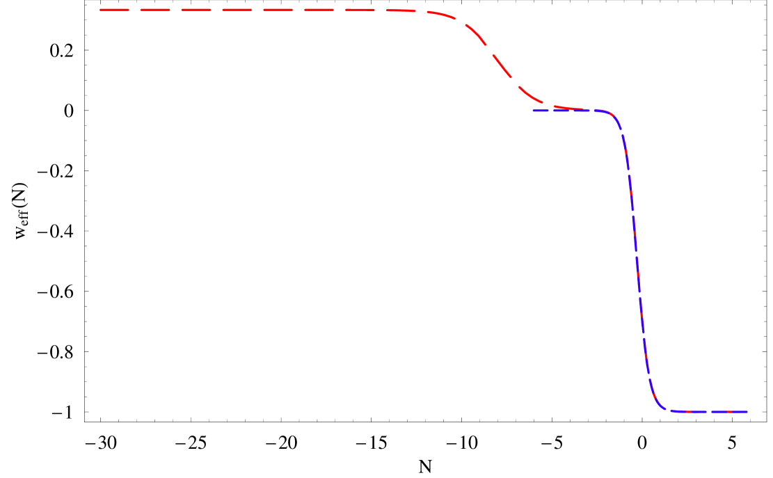
Figure 1: The effective equation of state $w_{eff}(N)$ imposed on the dynamical system (obtained from (24) using (26)). The long dashed red line starts deep in the radiation era while the short dashed blue line starts in the matter era and ignores radiation ($\Omega_{0r}=0$).

The ‘standard’ critical points are shown in Table III and they are the only critical points that have in addition to the correct expansion rate properties, the required values of $(\Omega_{r},\Omega_{m},\Omega_{DE})$ in each era. As shown in the next section these saddle critical points reconstruct the general relativistic $f(R)$ ie $f(R)=R-2\Lambda$. It is therefore clear that nonlinear $f(R)$ theories can produce an observationally acceptable cosmic history but not with the required values of $(\Omega_{r},\Omega_{m},\Omega_{DE})$ in each era. We should stress that our analysis has not excluded the possibility of physical values of $(\Omega_{0r},\Omega_{0{\rm m}},\Omega_{DE})$ in the case of cosmic histories oscillating around the anticipated $w_{eff}$ in each era or a $w_{eff}$ that is continuously evolving. These special cases however maybe severely constrained observationally.

To confirm the dynamical evolution implied by the ‘attractors’ of Table I, we have performed a numerical analysis of the dynamical system (17), (23), (19) using the ansatz (27) for $x_{3}$ with $\Omega_{0{\rm m}}=0.3$ and $\Omega_{0r}=10^{-4}$. This ansatz for $x_{3}(N)$ leads to the $w_{eff}(N)$ shown in Fig. 1. We have set up the system initially, close to the ‘standard’ radiation era saddle point $(0,0,0,1)$ and allowed it to evolve. As seen in Fig. 2 and Fig. 3 much before the onset of the matter era ($N\equiv N_{rr}\simeq-25<-8\simeq N_{rm}$) the slow (but non-zero) evolution of $x_{3}(N)$ forces the phase space trajectory to depart from the saddle point $(0,0,0,1)$ and head towards the radiation era stable ‘attractor’ $(-4,5,0,0)$ where it stays throughout the rest of the radiation era ($w_{eff}\simeq\frac{1}{3}$).

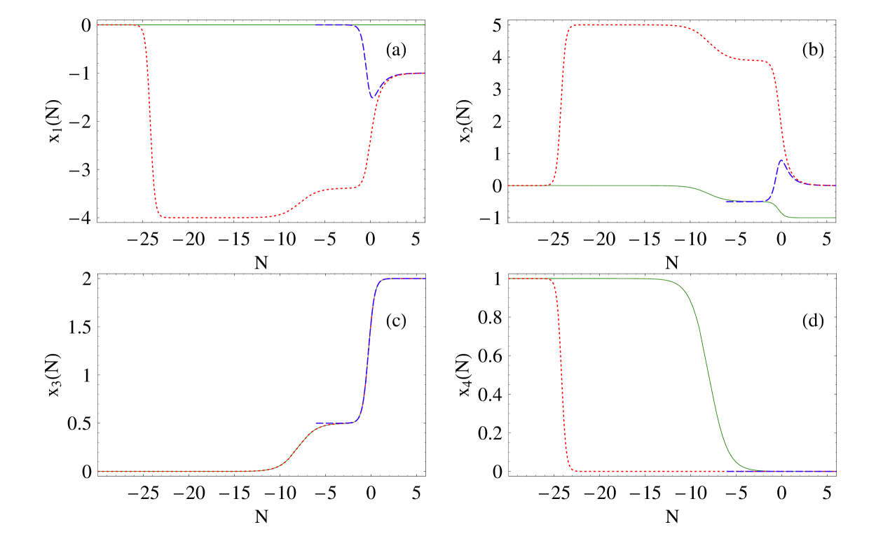
Figure 2: The evolution of the variables $x_{1}(N)$, $x_{2}(N)$, $x_{3}(N)$ and $x_{4}(N)$ for ‘standard’ radiation era initial conditions (dotted red line) and ‘standard’ matter era initial conditions (dashed blue line). The perturbed trajectories are rapidly dragged by the stable ‘attractors’ of each era. The numerically obtained evolution along the ‘standard’ saddle points of Table III is also shown (continuous green line). The instabilities of this trajectory are bypassed by using the constrained system (32)-(33) instead of the full system (17), (23), (22).

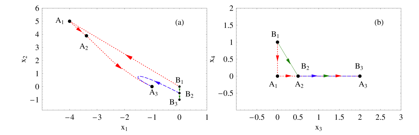
Figure 3: The phase space trajectories on the $x_{1}-x_{2}$ plane (Fig3a) and $x_{3}-x_{4}$ plane (Fig3b) for ‘standard’ radiation era initial conditions (dotted red line) and ‘standard’ matter era initial conditions (dashed blue line). The trajectory corresponding to the numerically obtained evolution along the saddle points of Table III is also shown (continuous green line). The points $A_{1}$, $A_{2}$, $A_{3}$ correspond to the ‘attractors’ of each era (radiation, matter and deSitter respectively) while the points $B_{1}$, $B_{2}$, $B_{3}$ correspond to the ‘standard’ critical points of each era (see Tables II and III). Notice that on the projection of Fig. 3b the ‘attractor’ points $A_{2}$, $A_{3}$ coincide with the ‘standard’ critical points $B_{2}$, $B_{3}$.

Subsequently, when $x_{3}(N)$ enters the matter era ($w_{eff}=0$) at $N_{rm}\simeq-8$, the trajectory follows the evolution of the ‘attractor’ fixed point and heads towards the matter era ‘attractor’ $(-3.386,3.886,0.5,0)$ ignoring the saddle point $(0,-1/2,1/2,0)$ of the ‘standard’ matter era. Finally when the matter era is over, the trajectory heads towards the deSitter ‘attractor’ $(-1,0,2,0)$ which is also distinct from the ‘standard’ deSitter saddle point $(0,-1,2,0)$. Notice that the deSitter ‘attractor’ is inconsistent with observations due to the implied large variation of the effective Newton’s constant $G(N)=\frac{1}{F(N)}$ even though this inconsistency could be ameliorated by ‘chameleon’ type mechanisms Khoury:2003rn . The evolution of $(\Omega_{r},\Omega_{m},\Omega_{DE})$ corresponding to the phase space trajectories of Figs. 2 and 3 is shown in Fig. 4a. Notice that $\Omega_{m}=0$ throughout the ‘attractor’ evolution of the system and the $w_{eff}=0$ of the matter era is induced by curvature dark gravity excitations.

We have also tested initial conditions in the matter era starting the evolution on the saddle point $(0,-\frac{1}{2},\frac{1}{2},0)$ corresponding to the ‘standard’ matter era. In this case we also ignore radiation setting $\Omega_{0r}=0$. We get an evolution of the system (see Figs 2, 3, 4b) which stays on the ‘standard’ matter era $\Omega_{m}=1$ for about 3 expansion times but before the onset of the acceleration era it gets absorbed by the ‘attractor’ towards the nonstandard deSitter critical point $(-1,0,2,0)$.

The above evolution along the ‘attractor’ critical points is a result of the ‘physical law’ $f(R)$ perturbations. We can also reproduce trajectories that go through critical points that are not stable by turning off these perturbations. For example we can recover the saddle critical point sequence

$$(0,0,0,1)\rightarrow(0,\frac{1}{2},-\frac{1}{2},0)\rightarrow(0,-1,2,0)$$ (31)

by fixing $x_{1}=0$ in the system (17), (23), (19) and reducing it to the system

$$-1-x_{3}-3x_{2}+x_{4} = 0$$ (32)

$$-2x_{3}x_{4} = x_{4}^{\prime}$$ (33)

which can be easily solved using the ansatz (27)

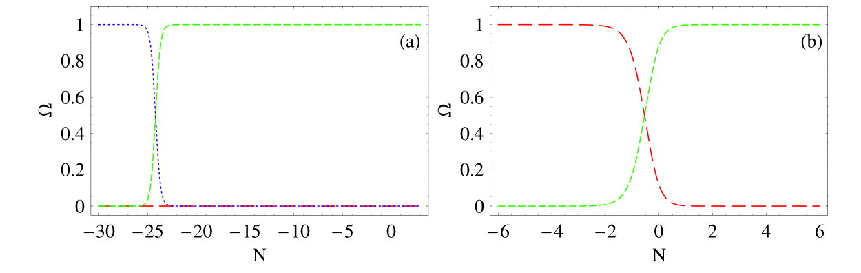
Figure 4: The evolution of $\Omega_{m}$ (long-dashed), $\Omega_{rad}$ (dotted) and $\Omega_{DE}$ (short-dashed) parameters for ‘standard’ radiation era initial conditions (Fig4a) and ‘standard’ matter era initial conditions (Fig4b). In both cases the ‘attractor’ critical points of Table II rapidly take over and drag the trajectories.

(see Fig. 2 and Fig. 3). The alternative approach of solving the decoupled pair (20), (19) does not lead to the correct result because the $f(R)$ perturbations are not turned off and the constraint is not respected in this case.

It is straightforward to reconstruct the functions $f(R)$ that correspond to the saddle general relativistic trajectory (31) and to the ‘attractor’ sequence of Table II. The functional forms of $f(R)$ may also be reconstructed on any one of the critical points of Table I. These tasks are undertaken in the next section.

III Reconstruction of $f(R)$

We now reconstruct the form of the function $f(R)$ that corresponds to each one of the critical points of the system shown in Table I. This reconstruction is effectively an approximation of $f(R)$ in the neighborhood of each critical point. It is particularly useful because most of the dynamical evolution takes place close to the fixed points. Consider a critical point of the form $({\bar{x}}_{1},{\bar{x}}_{2},{\bar{x}}_{3},{\bar{x}}_{4})$. Using (10) we find

$$F=F_{0}e^{-{\bar{x}}_{1}N}$$ (34)

where $F_{0}$ is a constant. We may eliminate $N$ in favor of $R$ using the input form of $H(N)$ (equation (26) in (14) to obtain (setting $H_{0}^{2}=1$)

$$R(N)=3\left[4\Omega_{\Lambda}+\Omega_{0{\rm m}}e^{-3N}\right]$$ (35)

which leads to

$$F=F_{0}\left(\frac{R-12\Omega_{\Lambda}}{3\Omega_{0{\rm m}}}\right)^{\frac{{\bar{x}}_{1}}{3}}$$ (36)

and by integration we get

$$f(R)=\frac{3F_{0}(3\Omega_{0{\rm m}})^{-\frac{{\bar{x}}_{1}}{3}}(R-12\Omega_{\Lambda})^{\frac{{\bar{x}}_{1}}{3}+1}}{{\bar{x}}_{1}+3}+f_{0}$$ (37)

where $f_{0}$ is an integration constant. Expressing (37) in terms of $N$ using (35) we obtain

$$f(N)=\frac{9F_{0}\Omega_{0{\rm m}}e^{-({\bar{x}}_{1}+3)N}}{{\bar{x}}_{1}+3}+f_{0}$$ (38)

It is now straightforward to use the expressions for $f(N)$ $R(N)$ and $H(N)$ to find $x_{2}(N)$ (equation (11)), $x_{3}(N)$ (equation (27)) and $x_{4}(N)$ (equation (13)). We thus find

$$x_{2}(N)=-\frac{\left(\frac{3\Omega_{0{\rm m}}}{2({\bar{x}}_{1}+3)}e^{-3N}+\frac{f_{0}}{6F_{0}}e^{{\bar{x}}_{1}N}\right)}{\Omega_{0{\rm m}}e^{-3N}+\Omega_{0r}e^{-4N}+\Omega_{\Lambda}}$$ (39)

and

$$x_{4}(N)=\frac{\Omega_{0r}e^{({\bar{x}}_{1}-4)N}}{F_{0}(\Omega_{0{\rm m}}e^{-3N}+\Omega_{0r}e^{-4N}+\Omega_{\Lambda})}$$ (40)

while $x_{3}(N)$ is given by (27). Using equations (39), (27) and (40) we may verify the ${\bar{x}}_{2}$, ${\bar{x}}_{3}$, ${\bar{x}}_{4}$ values of each critical point by considering the appropriate range of $N$ in each era and the corresponding value of ${\bar{x}}_{1}$. By demanding consistency with the values of Table I we may obtain the values of the constants $f_{0}$ and $F_{0}$.

As an example let’s consider the sequence (31) corresponding to the ‘standard’ cosmological eras (Table III). It is easy to see, using ${\bar{x}}_{1}=0$ and the appropriate range of $N$ in (39), (27) and (40) that we obtain the correct values for ${\bar{x}}_{2}$, ${\bar{x}}_{3}$, ${\bar{x}}_{4}$ in the radiation and matter eras for any value of $F_{0}$, $f_{0}$. In the deSitter era ($N>>1$) the value of $f_{0}$ needs to be fixed to get agreement with ${\bar{x}}_{2}=-1$ of Table I. In particular from (39) we find

$${\bar{x}}_{2}=-\frac{f_{0}}{6F_{0}\Omega_{\Lambda}}=-1$$ (41)

which implies

$$f_{0}=6F_{0}\Omega_{\Lambda}$$ (42)

Using now (42) and setting ${\bar{x}}_{1}=0$ in (37) we reconstruct the expected result

$$f(R)=F_{0}(R-6\Omega_{\Lambda})$$ (43)

which is valid for all three eras since in this sequence the value of ${\bar{x}}_{1}$ remains constant. In a similar way we may reconstruct $f(R)$ for any critical point in one of the three eras.

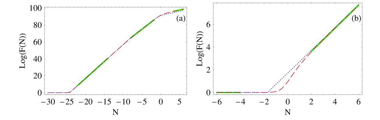
Figure 5: The form of $log(F(N))$ in the numerical reconstruction (dashed lines) and its analytical approximation using both the interpolating steps 1-3 (dotted lines) and the application of the analytical expression (38) valid in each era (thick green lines). The agreement between the three approaches is very good. 5a: ‘standard’ radiation era initial condition, 5b: ‘standard’ matter era initial condition.

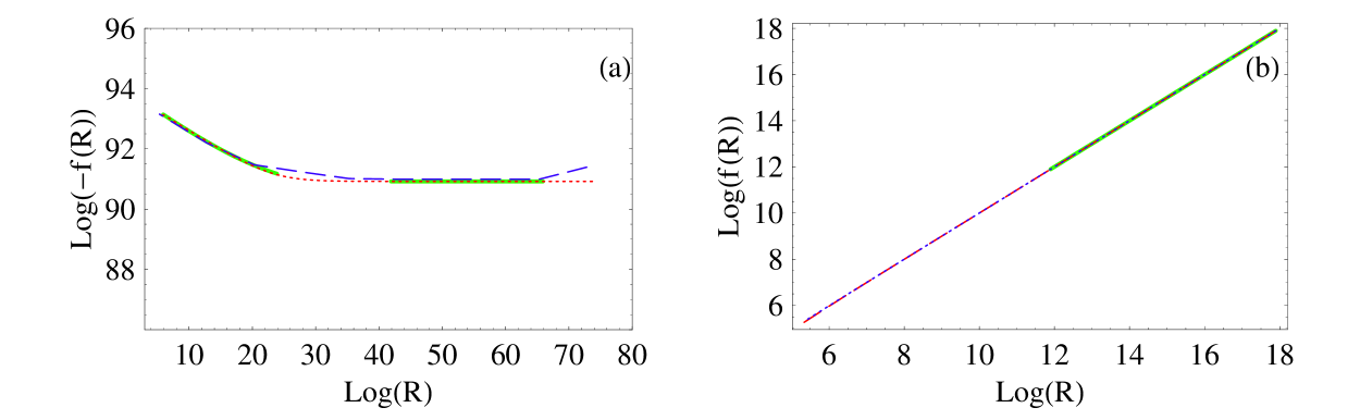
Figure 6: The form of $f(R)$ in the numerical reconstruction (dashed lines) and its analytical approximation using both the interpolating steps 1-3 (dotted lines) and the application of the analytical expression (37) valid in each era (continuous green lines). 6a: ‘standard’ radiation era initial condition with the continuous green lines corresponding to radiation era (larger $R$) and matter era (smaller $R$). The deSitter era is not shown since it corresponds to a single point (constant $R$). 6b: ‘standard’ matter era initial condition with the continuous green line corresponding to matter era. The deSitter era is not shown since it corresponds to a point (constant $R$).

We have therefore extended previous studies showing that $f(R)$ theories can only be viable in very restricted cases by showing that even these restricted cases can not reproduce a viable $\Lambda$CDM cosmology where $w_{eff}$ is constant during the matter and radiation eras and $\Omega_{0r}$, $\Omega_{m}$ take their cosmologically anticipated values. It therefore becomes clear that if the accelerating expansion of the universe is due to physics in the gravitational sector it may probably have to be a more general theory than $f(R)$ modified gravity. Such a theory could very well be scalar-tensor gravity (or equivalently coupled dark energycoupled ) whose cosmological dynamical properties and constraints need to investigated in detail.

In the case of sequence of transitions among critical points which involve different values of ${\bar{x}}_{1}$ the reconstruction can be done by either numerical determination of $x_{1}(N)$ or by approximating it as a sequence of step functions. For example, the steps involved in the reconstruction of the ‘attractor’ trajectory shown in Fig. 2 and Fig. 3 are the following:

1. Use (10) along with the numerical solution $x_{1}(N)$ to find the function $F(N)=f,_{R}(N)$ as

   $$F(N)=F_{0}e^{-\int_{N_{min}}^{N}x_{1}(N^{\prime})dN^{\prime}}$$ (44)

   The numerical solution $x_{1}(N)$ of Fig. 2a can be approximated as a piecewise constant function with values determined by the corresponding ‘attractors’ of each cosmological era and by the initial conditions ie

   $$x_{1}(N) = 0\;\;\;-30<N<N_{rr}$$ (45)

   $$x_{1}(N) = -4\;\;\;N_{rr}<N<N_{rm}$$ (46)

   $$x_{1}(N) = -3.386\;\;\;N_{rm}<N<N_{m\Lambda}$$ (47)

   $$x_{1}(N) \simeq -1\;\;\;\;N_{m\Lambda}<N$$ (48)

   (where $N_{rr}\simeq-25$) thus leading to an analytical approximation for $F(N)$. The resulting form of $\ln(F(N))$ in both the numerical reconstruction and its analytical approximation is shown in Fig. 5 (5a: ‘standard’ radiation era initial condition, 5b: ‘standard’ matter era initial condition).

2. Use equation (11) to find $f(N)$ from $F(N)$ ie

   $$f(N)=-6x_{2}(N)F(N)H(N)^{2}$$ (49)

   where $H(N)$ is given by (26), $x_{2}(N)$ is numerically obtained and shown in Fig. 2b and $F(N)$ is obtained in the previous step. As in the case of $x_{1}(N)$, $x_{2}(N)$ can be analytically approximated as

   $$x_{2}(N) = 0\;\;\;-30<N<N_{rr}$$ (50)

   $$x_{2}(N) = 5\;\;\;N_{rr}<N<N_{rm}$$ (51)

   $$x_{2}(N) = 3.886\;\;\;N_{rm}<N<N_{m\Lambda}$$ (52)

   $$x_{2}(N) \simeq 0\;\;\;\;N_{m\Lambda}<N$$ (53)

   using the corresponding ‘attractors’ to obtain an analytical expression for $f(N)$.

3. The resulting form of $f(N)$ can then be combined with equation (35) for $R(N)$ to reconstruct the function $f(R)$. The resulting form of $f(R)$ is shown in Fig. 6 for both the numerical reconstruction and its analytical approximation (6a: radiation era initial conditions, 6b: matter era initial conditions).

We can fit the reconstructed $f(R)$ of Figs. 6a and 6b to the analytic form of equation (37) for each era respectively so as to find the parameters $F_{0}$, ${\bar{x}}_{1}$ and $f_{0}$. The results are shown in Table IV.

Table 4: The parameters $F_{0}$, ${\bar{x}}_{1}$ and $f_{0}$ for the reconstructed $f(R)$ of Figs. 6a and 6b .

Radiation Era cond.	${\bar{x}}_{1}$	$Log(F_{0})$	$Log(-f_{0})$
Radiation Era	-3.99	96.73	90.92
Matter Era	-3.45	92.17	90.59
deSitter era	-1.01	92.62	94.03
Matter Era cond.	${\bar{x}}_{1}$	$F_{0}$	$f_{0}$
Matter Era	0	1	-1.51
deSitter era	-1.02	4.83	-16.56

Notice that the best fit values of ${\bar{x}}_{1}$ coincide with the corresponding ‘attractor’ critical points of Table II as expected. This verifies the validity of the reconstructed $f(R)$ expression from (37). A similar reconstruction analysis can be performed for any other sequence of critical points. As discussed in section II any such sequence is equally interesting cosmologically since the existence of the ‘attractor’ is an artifact of the $f(R)$ perturbations.

IV Conclusion-Outlook

We have shown analytically and numerically that nonlinear $f(R)$ gravity theories can reproduce the background expansion history $H(z)$ indicated by observations even when $f(R)$ does not reduce to general relativity at early times. In that case the universe gets dominated by dark gravity during its evolution as opposed to radiation or matter. This result relies on the values of all the critical points we found assuming only that the radiation era corresponds to a constant effective equation of state parameter $w_{eff}=\frac{1}{3}$ while for the matter era we have $w_{eff}=0$.

Our analysis indicates $f(R)$ models can be viable if $f(R)$ deviates from general relativity at early times. Thus a viable $f(R)$ theory must satisfy one of the following:

• Either $f(R)$ reduces to general relativity at early times, but departs from general relativity at late times (a well known casefRpapers ).

• Or dark gravity in the forms derived in our paper mimics radiation or matter at both the background level and the perturbative level. The later would clearly require a separate analysis of perturbations of the model.

Numerical Analysis: The mathematica files with the numerical analysis of this study may be found at http://leandros.physics.uoi.gr/frlcdm/frlcdm.htm or may be sent by e-mail upon request.

Acknowledgements: This work was supported by the European Research and Training Network MRTPN-CT-2006 035863-1 (UniverseNet). S.F. is supported by a Marie Curie Intra-European Fellowship of the European Union (contract number MEIF-CT-2005-515028). S.N. acknowledges support from the Greek State Scholarships Foundation (I.K.Y.).

References

- (1) S. Perlmutter et al., Astrophys. J. 517, 565 (1999); A. G. Riess et al., Astron. J. 116, 1009 (1998); Astron. J. 117, 707 (1999); J. L. Tonry et al., Astrophys. J. 594, 1 (2003); R. A. Knop et al., Astrophys. J. 598, 102 (2003); P. Astier et al., Astron. Astrophys. 447, 31 (2006); G. Miknaitis et al., arXiv:astro-ph/0701043; A. G. Riess et al., arXiv:astro-ph/0611572.
- (2) D. N. Spergel et al., Astrophys. J. Suppl. 148, 175 (2003); D. N. Spergel et al., arXiv:astro-ph/0603449.
- (3) D. J. Eisenstein et al., Astrophys. J. 633, 560 (2005); C. Blake, D. Parkinson, B. Bassett, K. Glazebrook, M. Kunz and R. C. Nichol, Mon. Not. Roy. Astron. Soc. 365, 255 (2006).
- (4) E. J. Copeland, M. Sami and S. Tsujikawa, arXiv:hep-th/0603057, to appear in Int. J. Mod. Phys. D.
- (5) V. Sahni and A. A. Starobinsky, Int. J. Mod. Phys. D 9, 373 (2000); S. M. Carroll, Living Rev. Rel. 4, 1 (2001); T. Padmanabhan, Phys. Rept. 380, 235 (2003); P. J. E. Peebles and B. Ratra, Rev. Mod. Phys. 75, 559 (2003); V. Sahni, Lect. Notes Phys. 653, 141 (2004) [arXiv:astro-ph/0403324]; L. Perivolaropoulos, AIP Conf. Proc. 848, 698 (2006) [arXiv:astro-ph/0601014]; J. P. Uzan, arXiv:astro-ph/0605313.
- (6) Y. Fujii, Phys. Rev. D 26, 2580 (1982); L. H. Ford, Phys. Rev. D 35, 2339 (1987); C. Wetterich, Nucl. Phys B. 302, 668 (1988); B. Ratra and J. Peebles, Phys. Rev D 37, 321 (1988); Y. Fujii and T. Nishioka, Phys. Rev. D 42, 361 (1990); E. J. Copeland, A. R. Liddle, and D. Wands, Ann. N. Y. Acad. Sci. 688, 647 (1993); C. Wetterich, A&A 301, 321 (1995); P. G. Ferreira and M. Joyce, Phys. Rev. Lett. 79, 4740 (1997); Phys. Rev. D 58, 023503 (1998); R. R. Caldwell, R. Dave and P. J. Steinhardt, Phys. Rev. Lett. 80, 1582 (1998); I. Zlatev, L. M. Wang and P. J. Steinhardt, Phys. Rev. Lett. 82, 896 (1999); P. J. Steinhardt, L. M. Wang and I. Zlatev, Phys. Rev. D 59, 123504 (1999); L. Perivolaropoulos, Phys. Rev. D 71, 063503 (2005) [arXiv:astro-ph/0412308].
- (7) N. Bilic, G. B. Tupper and R. D. Viollier, Phys. Lett. B 535, 17 (2002) [arXiv:astro-ph/0111325]; M. C. Bento, O. Bertolami and A. A. Sen, Phys. Rev. D 66, 043507 (2002) [arXiv:gr-qc/0202064].
- (8) A. Friedland, H. Murayama and M. Perelstein, Phys. Rev. D 67, 043519 (2003) [arXiv:astro-ph/0205520].
- (9) M. Li, Phys. Lett. B 603, 1 (2004) [arXiv:hep-th/0403127]; Q. G. Huang and Y. G. Gong, JCAP 0408, 006 (2004) [arXiv:astro-ph/0403590]; S. Nojiri and S. D. Odintsov, Gen. Rel. Grav. 38, 1285 (2006) [arXiv:hep-th/0506212]; M. R. Setare, Phys. Lett. B 644, 99 (2007) [arXiv:hep-th/0610190]; S. Nojiri and S. D. Odintsov, Gen. Rel. Grav. 38, 1285 (2006) [arXiv:hep-th/0506212].
- (10) B. Boisseau, G. Esposito-Farèse, D. Polarski and A. A. Starobinsky, Phys. Rev. Lett. 85, 2236 (2000); G. Esposito-Farèse and D. Polarski, Phys. Rev. D 63 063504 (2001);
- (11) J. P. Uzan, Phys. Rev. D 59, 123510 (1999) [arXiv:gr-qc/9903004]; Y. Fujii, Phys. Rev. D62, 044011 (2000); N. Bartolo and M. Pietroni, Phys. Rev. D 61 023518 (2000); F. Perrotta, C. Baccigalupi and S. Matarrese, Phys. Rev. D 61, 023507 (2000); D. F. Torres, Phys. Rev. D 66, 043522 (2002); R. Gannouji, D. Polarski, A. Ranquet and A. A. Starobinsky, JCAP 0609, 016 (2006); S. Capozziello, S. Nojiri and S. D. Odintsov, Phys. Lett. B 634, 93 (2006) [arXiv:hep-th/0512118]; A. Riazuelo and J. P. Uzan, Phys. Rev. D 66, 023525 (2002) [arXiv:astro-ph/0107386].
- (12) S. Nojiri and S. D. Odintsov, Gen. Rel. Grav. 36, 1765 (2004); M. E. Soussa and R. P. Woodard, Gen. Rel. Grav. 36, 855 (2004); G. Allemandi, A. Borowiec and M. Francaviglia, Phys. Rev. D 70, 103503 (2004); D. A. Easson, Int. J. Mod. Phys. A 19, 5343 (2004); S. M. Carroll, A. De Felice, V. Duvvuri, D. A. Easson, M. Trodden and M. S. Turner, Phys. Rev. D 71, 063513 (2005); S. Carloni, P. K. S. Dunsby, S. Capozziello and A. Troisi, Class. Quant. Grav. 22, 4839 (2005); S. Capozziello, V. F. Cardone and A. Troisi, Phys. Rev. D 71, 043503 (2005); G. Cognola, E. Elizalde, S. Nojiri, S. D. Odintsov and S. Zerbini, JCAP 0502, 010 (2005); A.F. Zakharov et al., Phys. Rev. D 74, 107101 (2006); J. A. R. Cembranos, Phys. Rev. D 73, 064029 (2006) [arXiv:gr-qc/0507039]; S. Nojiri, S. D. Odintsov and S. Tsujikawa, Phys. Rev. D 71, 063004 (2005); M. C. B. Abdalla, S. Nojiri and S. D. Odintsov, arXiv:hep-th/0601213; R. P. Woodard, arXiv:astro-ph/0601672; S. Das, N. Banerjee and N. Dadhich, Class. Quant. Grav. 23, 4159 (2006); S. Capozziello, V. F. Cardone, E. Elizalde, S. Nojiri and S. D. Odintsov, Phys. Rev. D 73, 043512 (2006); S. K. Srivastava, arXiv:astro-ph/0602116; T. P. Sotiriou, Class. Quant. Grav. 23, 5117 (2006); arXiv:gr-qc/0611107; arXiv:gr-qc/0611158; T. P. Sotiriou and S. Liberati, arXiv:gr-qc/0604006; A. De Felice, M. Hindmarsh and M. Trodden, JCAP 0608, 005 (2006); S. Bludman, arXiv:astro-ph/0605198; S. M. Carroll, I. Sawicki, A. Silvestri and M. Trodden, arXiv:astro-ph/0607458; D. Huterer and E. V. Linder, arXiv:astro-ph/0608681; X. h. Jin, D. j. Liu and X. z. Li, arXiv:astro-ph/0610854; N. J. Poplawski, Phys. Rev. D 74, 084032 (2006); arXiv:gr-qc/0610133; V. Faraoni, arXiv:astro-ph/0610734; T. Chiba, T. L. Smith and A. L. Erickcek, arXiv:astro-ph/0611867; V. Faraoni and S. Nadeau, arXiv:gr-qc/0612075; I. Navarro and K. Van Acoleyen, arXiv:gr-qc/0611127; A. W. Brookfield, C. van de Bruck and L. M. H. Hall, Phys. Rev. D 74, 064028 (2006); S. Fay, R. Tavakol and S. Tsujikawa, arXiv:astro-ph/0701479; M. Fairbairn and S. Rydbeck, arXiv:astro-ph/0701900; R. Dick, Gen. Rel. Grav. 36 (2004) 217 [arXiv:gr-qc/0307052]; S. Capozziello, S. Carloni and A. Troisi, [arXiv:astro-ph/0303041]; I. Sawicki and W. Hu, arXiv:astro-ph/0702278; T. Multamaki and I. Vilja, Phys. Rev. D 73, 024018 (2006) [arXiv:astro-ph/0506692].
- (13) R. Maartens, Living Rev. Rel. 7, 7 (2004) [arXiv:gr-qc/0312059]; V. Sahni and Y. Shtanov, JCAP 0311, 014 (2003) [arXiv:astro-ph/0202346]; G. Kofinas, G. Panotopoulos and T. N. Tomaras, JHEP 0601, 107 (2006) [arXiv:hep-th/0510207]; P. S. Apostolopoulos and N. Tetradis, Phys. Rev. D 74, 064021 (2006) [arXiv:hep-th/0604014]; C. Bogdanos, A. Dimitriadis and K. Tamvakis, arXiv:hep-th/0611094.
- (14) L. Perivolaropoulos, JCAP 0510, 001 (2005) [arXiv:astro-ph/0504582]; S. Nesseris and L. Perivolaropoulos, Phys. Rev. D 75, 023517 (2007) [arXiv:astro-ph/0611238]; J. Martin, C. Schimd and J. P. Uzan, Phys. Rev. Lett. 96, 061303 (2006) [arXiv:astro-ph/0510208]; R. Gannouji, D. Polarski, A. Ranquet and A. A. Starobinsky, JCAP 0609, 016 (2006) [arXiv:astro-ph/0606287].
- (15) U. Alam, V. Sahni, T. D. Saini and A. A. Starobinsky, Mon. Not. Roy. Astron. Soc. 354, 275 (2004) [arXiv:astro-ph/0311364]; S. Nesseris and L. Perivolaropoulos, Phys. Rev. D 72, 123519 (2005) [arXiv:astro-ph/0511040]; S. Nesseris and L. Perivolaropoulos, arXiv:astro-ph/0610092; R. Lazkoz, S. Nesseris and L. Perivolaropoulos, JCAP 0511, 010 (2005) [arXiv:astro-ph/0503230]; S. Nesseris and L. Perivolaropoulos, Phys. Rev. D 70, 043531 (2004) [arXiv:astro-ph/0401556].
- (16) N. D. Birrell, P. C. W. Davies, Quantum Fields in Curved Space, Cambridge University Press, Cambridge (UK) (1982); I. L. Buchbinder, S. D. Odintsov and I. L. Shapiro, Effective Action in Quantum Gravity, IOP, Bristol/Philadelphia (1992).
- (17) S. D. Odintsov, S. Nojiri, Phys. Lett. B 576, 5 (2003).
- (18) S. M. Carroll, V. Duvvuri, M. Trodden and M. S. Turner, Phys. Rev. D 70, 043528 (2004).
- (19) S. Capozziello, S. Carloni, V. F. Cardone, A. Troisi, Int. J. Mod. Phys. D 12, 1969 (2003).
- (20) T. Chiba, Phys. Lett. B 575, 1 (2003).
- (21) A. D. Dolgov and M. Kawasaki, Phys. Lett. B 573, 1 (2003).
- (22) V. Faraoni, Phys. Rev. D 74, 023529 (2006); G. J. Olmo, Phys. Rev. Lett. 95, 261102 (2005) [arXiv:gr-qc/0505101].
- (23) E.V. Pitjeva, Astron. Lett. 31, 340 (2005); Sol. Sys. Res. 39, 176 (2005).
- (24) S. Nojiri and S. D. Odintsov, Phys. Rev. D 68, 123512 (2003).
- (25) L. Amendola, D. Polarski and S. Tsujikawa, arXiv:astro-ph/0603703.
- (26) S. Capozziello, S. Nojiri, S. D. Odintsov and A. Troisi, Phys. Lett. B 639, 135 (2006) [arXiv:astro-ph/0604431]; S. Nojiri and S. D. Odintsov, Phys. Rev. D 74, 086005 (2006) [arXiv:hep-th/0608008]; S. Nojiri and S. D. Odintsov, arXiv:hep-th/0610164.
- (27) L. Amendola, R. Gannouji, D. Polarski and S. Tsujikawa, arXiv:gr-qc/0612180.
- (28) This type of evolution would be more likely if we had found complex eigenvalues for the saddle point which would allow for oscillations around the correct matter era.
- (29) J. Khoury and A. Weltman, Phys. Rev. D 69, 044026 (2004) [arXiv:astro-ph/0309411]; B. Li and J. D. Barrow, [arXiv:gr-qc/0701111]; D. F. Mota and J. D. Barrow, Mon. Not. Roy. Astron. Soc. 349, 291 (2004) [arXiv:astro-ph/0309273].
- (30) L. Amendola, Phys. Rev. D 62, 043511 (2000); L. Amendola and D. Tocchini-Valentini, Phys. Rev. D 64, 043509 (2001); L. Amendola and C. Quercellini, Phys. Rev. D 68, 023514 (2003).