Exact Solutions of Regge-Wheeler Equation

Abstract

The Regge-Wheeler equation describes the axial perturbations of Schwarz- schild metric in linear approximation. We present its exact solutions in terms of the confluent Heun’s functions, the basic properties of the general solution, novel analytical approach and numerical techniques for study of different boundary problems which correspond to quasi-normal modes of black holes and other simple models of compact objects. We depict in more detail the exact solutions of Regge-Wheeler equation in the Schwarzschild black hole interior and on Kruscal-Szekeres manifold.

1 Introduction

The well known Regge-Wheeler equation (RWE)

$$\partial_{t}^{2}\Phi_{s,l}+\left(-\partial^{2}_{x}+V_{s,l}\right)\Phi_{s,l}=0$$ (1.1)

describes the axial perturbations of Schwarzschild metric in linear approximation and plays an important role in modern perturbation treatment of Schwarzschild black hole (SBH) physics. Its study has a long history and significant achievements [2].

The effective potential in RWE (1.1) reads

$$V_{s,l}(r)=\left(1-{{1}\over r}\right)\left({{l(l+1)}\over{r^{2}}}+{{1-s^{2}}\over{r^{3}}}\right).$$

The area radius $r\geq 0$ can be expressed explicitly as a function of the ”tortoise” coordinate $x\!=\!r\!+\!r_{\!{}_{Sch}}\ln\left(|r/r_{\!{}_{Sch}}\!-\!1|\right)$ using Lambert W-function: $r=W(\pm e^{x-1})+1$. In the last formula sign $"+"$ stands for SBH exterior $r\in(1,\infty)$ and sign $"-"$ – for the SBH interior $r\in(0,1)$. Hereafter we are using units in which the Schwarzschild radius $r_{\!{}_{Sch}}\!=\!2M\!=\!1$. The most important case $s\!=\!2$ describes the gravitational waves and is our main subject here.

The ansatz $\Phi_{s,l}(t,r)=R_{\omega,s,l}(r)e^{i\omega t}$ brings us to the stationary problem in the outer domain $r>1$:

$$\partial^{2}_{x}R_{\omega,s,l}+\left(\omega^{2}-V_{s,l}\right)R_{\omega,s,l}=0.$$ (1.2)

Its exact solutions were described recently [3] in terms of the confluent Heun’s functions $HeunC\!\left(\alpha,\beta,\gamma,\delta,\eta,r\right)$ [4].

In the exterior domain the variable $r$ plays the role of 3D-space coordinate and the variable $t$ – the role of exterior time of a distant observer. Because of the change of the signs of the components $g_{tt}=-1/g_{rr}=1-1/r$ of the metric, in the inner domain the former Schwarzschild-time variable $t$ plays the role of radial space variable $r_{in}=t\in(0,\infty)$ and the area radius $r\in(1,0)$, plays the role of time variable. As a result, the Regge-Wheeler ”tortoise” coordinate $x\in(-\infty,0)$ presents a specific time coordinate in the inner domain. For the study of the solutions of (1.1) in this domain it is useful to stretch the last interval to the standard one by a further change of the time-variable: $x\to t_{in}=x-1/x\in(-\infty,\infty)$.

These notes are important for the physical interpretation of the mathematical results. In particular, the natural form of the interior solutions of (1.1) is

$$\Phi_{\omega,s,l}^{in}(r_{in},t_{in})=e^{i\omega r_{in}}R_{\omega,s,l}\left(r(t_{in})\right),$$

where

$$r(t_{in})\!=\!W\!\left(-exp\left({{t_{in}}\over{2}}\!-\!1\!-\!\sqrt{\left({{t_{in}}\over{2}}\right)^{2}\!+\!1}\,\right)\right)\!\!+\!1.$$

The dependence of this solution on the interior radial variable $r_{in}$ is simple. Its dependence on the interior time $t_{in}$ is governed by the (1.2) with interior-time-dependent potential $V_{s,l}$. In despite of this unusual feature of the solutions in the SBH interior, this way we obtain a basis of functions, which are suitable for the study of the corresponding linear perturbations.

2 Exact Solutions of Regge-Wheeler Equation in Terms of Confluent Heun’s functions

In $r$ variable the RWE reads:

$${{d^{2}R_{\omega,s,l}}\over{dr^{2}}}+{1\over{r(r-1)}}{{dR_{\omega,s,l}}\over{dr}}+$$ (2.1)

$${{\omega^{2}r^{4}-l(l+1)r^{2}+\left(l(l+1)+s^{2}-1\right)r+1-s^{2}}\over{r^{2}(r-1)^{2}}}R_{\omega,s,l}=0.$$

The anzatz $R_{\omega,s,l}(r)=r^{s+1}(r-1)^{i\omega}e^{i\omega r}H(r)$ reduces it to the confluent Heun equation [4]:

$${{d^{2}H}\over{dr^{2}}}+\left(\alpha+{{\beta+1}\over{r}}+{{\gamma+1}\over{r-1}}\right){{dH}\over{dr}}+\hskip 150.79968pt$$

$${1\over{r(r-1)}}\left(\Big{(}\delta+{1\over 2}\alpha(\beta+\gamma+2)\Big{)}r+\eta+{\beta\over 2}+{1\over 2}(\gamma-\alpha)(\beta+1)\right)H=0$$ (2.2)

with the specific parameters: $\alpha=2i\omega,\beta=2s,\gamma=2i\omega,\delta=2\omega^{2},\eta=s^{2}-l(l+1)$ and three singular points in the whole complex plane $\mathbb{C}_{r}$ [3]. Two of them: $r=0$ and $r=1$ are regular and can be treated on equal foods. The third one: $r=\infty$ is an irregular singular point. Note that after all the horizon $r=1$ turns to be a singular point in the above sense, nevertheless with respect to the algebraic invariants of the Riemann’s curvature tensor it does not define a singular surface in the very Schwarzschild space-time manifold $\mathbb{M}^{(1,3)}\{g_{ij}(t,r,\theta,\phi)\}$.

Correspondingly, one can write down three pairs of exact local solutions – one regular and one singular – around each singular point $X=0,1,\infty$:

1) Frobenius type of solutions around the points $r=0$ and $r=1$:

$$\Phi_{\,\,\omega,s,l}^{(0)\pm}(t,r)=e^{i\omega t}R_{\,\,\omega,s,l}^{(0)\pm}(r),\hskip 253.22934pt$$ (2.3a)

$$R_{\,\,\omega,s,l}^{(0)\pm}(r)=r^{s+1}e^{i\omega r+i\omega\ln(1-r)}\begin{cases}H_{\,\,\omega,s,l}^{(0)+}(r),\,\\ HeunC\!\left(2i\omega,2s,2i\omega,2\omega^{2},s^{2}-l(l+1),r\right);\end{cases}\hskip 17.07182pt$$ (2.3b)

$$\Phi_{\,\,\omega,s,l}^{(1)\pm}(t,r)=e^{i\omega t}R_{\,\,\omega,s,l}^{(1)\pm}(r),\hskip 247.53888pt$$ (2.4a)

$$R_{\,\,\omega,s,l}^{(1)\pm}(r)\!=\!r^{s+1}e^{i\omega r\pm i\omega\ln(r-1)}\times\hskip 224.7766pt$$

$$\hskip 85.35826ptHeunC\left(-2i\omega,\pm 2i\omega,2s,-2\omega^{2},2\omega^{2}+s^{2}-l(l+1),1-r\right)\!;$$ (2.4b)

2) Asymptotic Tome type of solutions around the point $r=\infty$:

$$\Phi_{\,\,\omega,s,l}^{(\infty)\pm}(t,r)=e^{i\omega t}R_{\,\,\omega,s,l}^{(\infty)\pm}(r),\hskip 241.84842pt$$ (2.5a)

$$R_{\,\,\omega,s,l}^{(\infty)\pm}(r)\sim{{e^{\mp i\omega r-i\omega\ln r}}}\sum_{\nu\geq 0}{{a_{\nu}^{\pm}}\over{r^{\nu}}},\,\,\,\,a_{0}^{\pm}=1.\hskip 179.25244pt$$ (2.5b)

These solutions describe ingoing and outgoing waves, associated with the corresponding singular point, according to the following scheme.

Table 1: In-out properties of local solutions.

Ingoing solutions:			Outgoing solutions:
$\Phi_{\,\,\omega,s,l}^{(0)+}(t,r):$	$0\leftarrow$		$\Phi_{\,\,\omega,s,l}^{(0)-}(t,r):$	$0\rightarrow$
$\Phi_{\,\,\omega,s,l}^{(1)+}(t,r):$	$1\leftarrow$		$\Phi_{\,\,\omega,s,l}^{(1)-}(t,r):$	$1\rightarrow$
$\Phi_{\,\,\omega,s,l}^{(\infty)+}(t,r):$	$\rightarrow\infty$		$\Phi_{\,\,\omega,s,l}^{(\infty)-}(t,r):$	$\leftarrow\infty$

The solutions own the following properties:

$$\lim_{r\to X}|\Phi_{\,\,\omega,s,l}^{(X)+}(t,r)| = \infty,$$ (2.6a)

$$\lim_{r\to X}|\Phi_{\,\,\omega,s,l}^{(X)-}(t,r)| = 0,$$ (2.6b)

with the important justification in the case $|\omega|>0$, as described by the equations

$$\lim_{|r|\to\infty}|R_{\,\,\omega,s,l}^{(\infty)+}(r)|=\begin{cases}\infty,\,\,\,&\hbox{if}\,\,\,\arg(r)+\arg(\omega)\in(0,\pi)/\hskip-11.38092pt\mod 2\pi;\\ 0,\,\,\,&\hbox{if}\,\,\,\arg(r)+\arg(\omega)\in(-\pi,0)/\hskip-11.38092pt\mod 2\pi.\end{cases}$$ (2.7a)

$$\lim_{|r|\to\infty}|R_{\,\,\omega,s,l}^{(\infty)-}(r)|=\begin{cases}0,\,\,\,&\hbox{if}\,\,\,\arg(r)+\arg(\omega)\in(0,\pi)/\hskip-11.38092pt\mod 2\pi;\\ \infty,\,\,\,&\hbox{if}\,\,\,\arg(r)+\arg(\omega)\in(-\pi,0)/\hskip-11.38092pt\mod 2\pi,\end{cases}$$ (2.7b)

and illustrated in Fig.1.

Figure 1: Domains of different behavior of the functions $R_{\,\,\omega,s,l}^{(\infty)\pm}(r)$.

The general solution of the RWE equation (1.2) can be represented in the form $R_{\omega,s,l}(r)=C_{X+}R_{\,\,\omega,s,l}^{(X)+}(r)+C_{X-}R_{\,\,\omega,s,l}^{(X)-}(r)$ with proper constants $C_{X\pm}$. The different local solutions are related according the formula

$$R_{\,\,\omega,s,l}^{(X)\pm}(r)=\Gamma_{\,Y+}^{X\pm}(\omega,s,l)R_{\,\,\omega,s,l}^{(Y)+}(r)+\Gamma_{\,Y-}^{X\pm}(\omega,s,l)R_{\,\,\omega,s,l}^{(Y)-}(r).$$

The main obstacle for pure analytical treatment of different interesting problems, related to the Regge-Wheeler equation, is that the transition coefficients $\Gamma_{\,Y\pm}^{X\pm}(\omega,s,l)$ for $X,Y=0,1,\infty$; $X\neq Y$ are not known explicitly.

3 Different Boundary Problems for the Stationary Regge-Wheeler Equation

Due to the existence of three singular points of RWE, we have three different two-singular-ends boundary problems [4] in the complex plane $\mathbb{C}_{r}$, Fig.2. These describe different physical problems, related with SBH exterior, SBH interior and Kruscal-Szekeres (KS) extension of the Schwarzschild solution [5].

Besides we can consider regular-singular-ends boundary problems on the interval $(r_{*},\infty)$, $r_{*}>1$ which can describe the perturbation of the metric around compact spherically symmetric matter objects in rest.

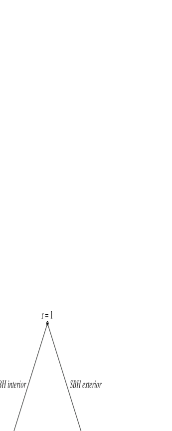
Figure 2: Different types of two-singular-ends boundary problems.

3.1 Perturbations of the SBH Exterior

Most well studied are the linear perturbations of the SBH exterior [1, 2]. Since the quasi-normal modes (QNM) are defined as a stable solutions of RWE (1.1) which describe pure ingoing waves both into the horizon $r=1$ and into the space infinity $r=\infty$, we can describe them using the solutions $R_{\,\,\omega,s,l}^{(1)+}(r)$ (2.4b) of (1.2), which obey the non-explicit equation $\Gamma_{\infty-}^{\,1\,\,+}(\omega,s,l)=0$. It yields the QNM frequencies $\omega=\omega(n,s,l),\,\,\,n=0,1,2,\dots$ . Our exact approach gives the spectral condition [3]:

$$\lim_{|r|\to+\infty}\bigg{|}\,r^{s+1}\!HeunC\left(\!-2i\omega,2i\omega,2s,-2\omega^{2},2\omega^{2}\!\!+\!s^{2}\!-\!l(l\!+\!1),1\!-\!|r|e^{\!-i\left(\!{\pi\over 2}\!+\!\arg(\omega)\right)}\!\right)\!\bigg{|}$$

$$=0.$$ (3.1)

It expresses in an explicit way the condition that the ingoing at the horizon waves do not contain coming from the infinity waves and can be solved numerically using the computer package Maple 10.

The equation (3.1) reproduces with a great precision the known numerical results, obtained by different methods [2]. For example, for the basic QNM-eigenvalue our calculations give $\omega(0,2,2)=0.747343368836+i\,0.177924631360$ [3], thus justifying the previously published results [2]. The first six eigenvalues are shown in Fig.8.

The amplitude of all QNM solutions $R_{\,\,\omega(n,s,l),s,l}^{(1)+}(r)$ increase infinitely around the horizon and near the space infinity, according to the (2.6a). This shows that Regge-Wheeler perturbation theory is not applicable in the corresponding vicinities of these points.

3.2 Perturbations of the SBH Interior

The perturbations of SBH interior were considered qualitatively for the first time in [6]. We present here an explicit exact treatment of the problem.

In the classical theory of BH it seems reasonable to exclude from the most of the considerations the inner domain, because it does not influence directly the observable outer domain. Nevertheless, the excitations of degrees of freedom in the inner domain may be essential for the consideration of the total BH entropy and for construction of the quantum theory of BH. The interior excitations may yield observable effects in the exterior of the BH, due to the quantum effects [7].

Another reason to study the BH interior was discovered in the recent article [8]: It was shown that without excision of the inner domain around the singularity one can improve dramatically the long-term stability of the numerical calculations. Although the region of the space-time that is causally disconnected can be ignored for signals and perturbations traveling at physical speeds, numerical signals, such as gauge waves or constraint violations, may travel at velocities larger then that of light and thus leave the physically disconnected region.

The perturbative treatment is related with the metric’s dynamics and corresponding initial value problem: using the field equation one has to determine the evolution of the initial data on a proper Cauchy surface. In the exterior domain solutions of (1.1), which grow up infinitely with respect to the future direction of the exterior time $t$ do exist. They are unstable and physically unacceptable. Therefore such solutions are excluded from any physical consideration [2, 1].

Then one has to formulate a proper boundary problem for (1.2), which has a reach variety of solutions and may describe different physical problems. For a correct formulation of a given physical problem one restricts the class of the solutions using proper boundary conditions. Since the physics at the boundary influences strongly the solutions of the problem, the boundary conditions are a necessary ingredient of the theory and define the physical problem under consideration. Only after that the physical problem is fixed and one can prove the stability of the remaining solutions (QNM) and small perturbations of general form with respect to the exterior-time evolution [9]. Our point is to consider different type of mathematical boundary problems, related with (1.2).

By analogy with the consideration in the outer domain of SBH, in the inner one we are considering only solutions, which are stable with respect to the future direction of the interior time. Therefore we study the solutions of (1.2), which are regular at the point $r\!=\!0$. These have a nontrivial spectrum with novel properties. Since we are working in the framework of perturbation theory, the presence of ”bad” solutions $R_{\,\,\omega,s,l}^{(0)+}(r)$, see (2.3b), which diverge and even are not single-valued, shows that, in general, two different types of situation can take place: either the considered here perturbation theory does not work in some domain around the interior-future infinity, or the full nonlinear problem has ”bad” solutions, which have to be excluded from the physical considerations using proper additional conditions. It is impossible to resolve this problem in the framework of the linear perturbation theory. Nevertheless, it is clear, that the opposite case of the regular solutions $R_{\,\,\omega,s,l}^{(0)-}(r)$, see (2.3b), has always a well defined physical meaning around future infinity of the interior time and deserves a corresponding study. For this purpose we are using a second pair of solutions around the horizon $r=1$:

$$\bar{R}_{\,\,\omega,s,l}^{(1)\pm}(r)\!=\!r^{s\!+\!1}e^{\!\pm i\omega\left(\ln(1\!-\!r)\!-r\right)}HeunC\!\left(\pm 2i\omega,\pm 2i\omega,2s,-2\omega^{2},2\omega^{2}\!\!+\!s^{2}\!\!-\!l(l\!+\!1),1\!-\!r\right)\!,\hskip 11.38092pt$$ (3.2)

which can be derived from the solutions (2.4b), applying proper transformations of the Heun’s functions [4]. For $\omega\neq 0$ the functions $\bar{R}_{\,\,\omega,s,l}^{(1)\pm}(r)$ (3.2) define a pair of linearly independent solutions with the symmetry property $\bar{R}_{\,\,\omega,s,l}^{(1)\pm}(r)=\bar{R}_{\,\,-\omega,s,l}^{(1)\mp}(r)$.

1. For real $\omega^{2}>0$ the problem has a real continuous spectrum. The corresponding solutions $R_{\omega,2,2}(t_{in})$ are illustrated in Fig.3. They define a basis of stable normal modes for perturbations of the metric in the SBH interior and can be used for Fourier expansion of perturbations of more general form.

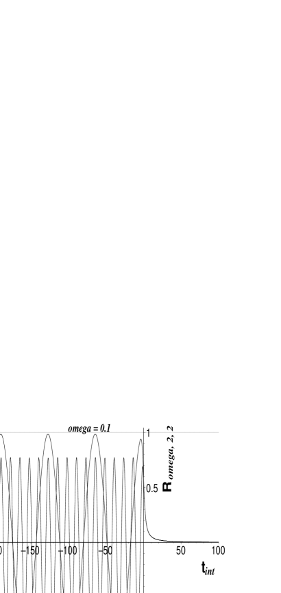
Figure 3: Two solutions of the continuous spectrum.

2. The zero eigenvalue $\omega=0$ yields a degenerate case in which the two functions (3.2) coincide. Then we obtain the infinite series of polynomial solutions:

$$R_{\,\,\omega=0,s,l}^{(0)-}(r)\!=\!{{(l\!-\!s)!}\over{Poch(1\!+\!2s,l\!-\!s)}}r^{s\!+\!1}JacobiP(l\!-\!s,2s,0,1\!-\!2r)=r^{3}\!+\!\dots,$$ (3.3)

which are finite on the whole interval $r\in[0,1]$. These functions form an orthogonal basis of stable normal modes. Here $JacobiP(n,a,b,z)$ stands for the standard Jacobi polynomials and $Poch(c,d)$ – for the Pochhammer symbol.

3. The discrete spectrum of the problem at hand corresponds to pure imaginary values of the parameter $\omega=i\omega_{I}$ [6, 3], i.e. to Laplace transform of the perturbations of general type. Thus, studying the the case $\omega^{2}<0$ we are constructing a basis for Laplace expansion of the perturbations of more general form in the SBH interior.

Then the functions $R_{\,\,\omega,s,l}^{(0)-}(r)$, $\bar{R}_{\,\,\omega,s,l}^{(1)\pm}(r)$ and all their parameters are real. In particular,

$$R_{\,\,\omega,s,l}^{(0)-}(r)\!=\!\Gamma_{1+}^{0-}(\omega,s,l)\bar{R}_{\,\,\omega,s,l}^{(1)+}(r)+\Gamma_{1-}^{0-}(\omega,s,l)\bar{R}_{\,\,\omega,s,l}^{(1)-}(r)$$ (3.4)

$$\hskip 46.94687pt\sim\cos\alpha\,\bar{R}_{\,\,\omega,s,l}^{(1)+}(r)+\sin\alpha\,\bar{R}_{\,\,\omega,s,l}^{(1)-}(r)\hskip 56.9055pt$$

with real transition coefficients $\Gamma_{1-}^{0\pm}(\omega,s,l)$ and real mixing angle $\alpha$, defined via the relation $\tan\alpha=\Gamma_{1-}^{0-}(\omega,s,l)/\Gamma_{1+}^{0-}(\omega,s,l)\in\mathbb{R}$ for $\omega=i\omega_{I}$.

The physical meaning of the mixing angle $\alpha$ is obvious: since the solutions $\bar{R}_{\,\,\omega,s,l}^{(1)+}(r)$ describe the ingoing into the horizon waves and the solutions $\bar{R}_{\,\,\omega,s,l}^{(1)-}(r)$ – the outgoing from the horizon waves, this angle describes the ratio of the amplitudes of these waves in their mixture (3.4). The value $\alpha=0$ corresponds to absence of outgoing waves (i.e. to the authentic SBH boundary conditions at the horizon). The value $\alpha=\pi/2$ describes the case without ingoing waves. The values $\alpha\in(0,\pi/2]$ describe an extension of the simple SBH problem in which the interior domain has a more general meaning then a pure SBH interior. Thus, fixing the value of the mixing angle $\alpha\in[0,\pi/2]$ we are defining completely a more wide class of problems than the traditional SBH.

Figure 4: The inverse potential $-V(r)$.

Figure 5: The first 18 eigenvalues (for n=0, 2,…,17, s=l=2 and $\alpha=0$).

The discrete imaginary spectrum can be obtained from the spectral equation:

$$\left|\begin{array}[]{cc}R_{\,\,\omega,s,l}^{(0)-}(r_{1})&\cos\alpha\,\bar{R}_{\,\,\omega,s,l}^{(1)+}(r_{1})\!+\!\sin\alpha\,\bar{R}_{\,\,\omega,s,l}^{(1)-}(r_{1})\\ R_{\,\,\omega,s,l}^{(0)-}(r_{2})&\cos\alpha\,\bar{R}_{\,\,\omega,s,l}^{(1)+}(r_{2})\!+\!\sin\alpha\,\bar{R}_{\,\,\omega,s,l}^{(1)-}(r_{2})\end{array}\right|=0,\hskip 17.07182pt$$ (3.7)

where $r_{1,2}\in(0,1),r_{1}\neq r_{2}$ are two otherwise arbitrary points. Because of the symmetry property of solutions $\bar{R}_{\,\,\omega,s,l}^{(1)\pm}(r)$, it is enough to study only the solutions $\omega_{n,s,l}$ of the equation (3.7) with positive $\omega_{I}=Im\left(\omega_{n,s,l}\right)>0$.

In the Fig.5 we see the first 18 eigenvalues (including the zero eigenvalue) of the RWE for SBH interior for $s=l=2$ and $\alpha=0$. The two series: $n=0,1,\dots 6$; and $n=7,\dots$, which correspond to the two wells of the inverse potential $-V(r)$, are clearly seen. They are placed around the straight lines $\omega_{I}=n/2+1/2$ and $\omega_{I}=n/2+1$, correspondingly.

In Fig.6 we see a specific attraction and repulsion of the eigenvalues $\omega_{n,s,l}(\alpha)$. Such behavior is typical for the eigenvalue problems related with the Heun’s equation [4]. It is well known in the quantum physics. To the best of our knowledge, this phenomenon is observed for the first time in the theory of the perturbations of Schwarzschild metric and needs further study to reach the corresponding physical understanding.

Figure 6: The dependence of $Im\left(\omega_{n,2,2}\right)$ on the mixing angle $\alpha\in[0,2\pi]$.

3.3 Perturbations of the Kruscal-Szekeres Manifold

To study the stable solutions of the first-order Regge-Wheeler perturbation theory in this case one has to choose the functions

$$R_{\,\,\omega,s,l}^{(0)-}(r)\!=\!\Gamma_{\infty+}^{0-}(\omega,s,l)R_{\,\,\omega,s,l}^{(\infty)+}(r)+\Gamma_{\infty-}^{0-}(\omega,s,l)R_{\,\,\omega,s,l}^{(\infty)-}(r),$$

which are regular at the interior-future-infinity $t_{int}=\infty$, and then to impose on them the condition $\Gamma_{\infty-}^{0-}(\omega,s,l)=0$. It is needed to annulate the waves, coming from the space infinity $r=\infty$. Making use of (2.3), (2.5) and (2.7), it is not hard to obtain the following explicit form of this condition:

$$\lim_{|r|\to\infty}\Big{|}r^{s+1}e^{2i\omega\ln r}HeunC(2i\omega,2s,2i\omega,2\omega^{2},s^{2}-l(l+1),r)\Big{|}_{r=|r|e^{-i({\pi\over 2}+arg\omega)}}\!=\!0.$$ (3.8)

Our numerical study of the case $s=l=2$ shows that this equation has no finite complex solutions $\omega$ with $|\omega|<\infty$. Hence, in this case all existing solutions of RWE with no waves coming from special infinity are growing infinitely when approaching the point $r=0$, i.e. they are unstable in direction of the interior future.

As an example of such solution one can consider the functions $R_{\,\,\omega,s,l}^{(1)-}(r)$. According to the (2.6b), when $Im(\omega)>0$ these functions are finite and continuous in the whole interval $r\in(0,\infty)$. They tend continuously to zero at both sides of the horizon $r=1$ (which in this case is a branching point in $\mathbb{C}_{r}$) and to infinity – when approaching the singular points $r=0$ and $r=\infty$. Unfortunately, these solutions contain both going to space infinity and coming from there waves. Our numerical study of the case $s=l=2$ shows that it is impossible to fulfill the condition

$$\Gamma_{\infty-}^{1-}(\omega,s,l)=\lim_{|r|\to\infty}\left.{{R_{\,\,\omega,s,l}^{(1)-}(r)}\over{R_{\,\,\omega,s,l}^{(\infty)-}(r)}}\right|_{r=|r|e^{-i(\pi/2+arg(\omega))}}=\hskip 142.26378pt$$ (3.9)

$$\lim_{|r|\to\infty}r^{1+s}HeunC(-2i\omega,2i\omega,2s,-2\omega^{2},s^{2}\!-\!l(l\!+\!1)\!+2\omega^{2},1-r)\Big{|}_{r=|r|e^{-i(\pi/2+arg(\omega))}}$$

$$=0,$$

which excludes the coming from the space infinity waves and is expecting to yield the corresponding spectrum of the frequencies $\omega$.

Another example are solutions $R_{\,\,\omega,s,l}^{(1)+}(r)$, considered in the whole interval $r\in(0,\infty)$. Our consideration in Section 3.1 shows that in this case one is able to exclude the coming from space infinity waves, obtaining this way the standard QNM frequencies. These solutions go to infinity both at the horizon and at the singular points $r=0$ and $r=\infty$. Hence, they are not stable in direction of the interior future and are not suitable for constructing perturbation theory in vicinity of all of the three singular points of the RWE.

3.4 Perturbations of the Exterior of Compact Matter Objects

Here we consider a one-parameter family of real intervals $(r_{\!*},\infty)\subset(1,\infty)$ with Dirichlet’s boundary condition at the left end: $\Phi_{\omega,s,l}(t,r_{\!*})=0$. Physically this means that the waves are experiencing a total reflection at the spherical surface with the area radius $r=r_{\!*}>1$, instead of going freely through it without any reflection, as in the case of black holes.

One can consider this surface as a boundary of some massive spherically symmetric body. Owing to the Birkhoff theorem, in general relativity the gravitational field of any massive body with Keplerian mass $M$ outside the radius $r_{\!*}$ coincides with the corresponding field of a black hole. Hence, the spreading of the waves in the outer domain of the massive body is governed by the Regge-Wheeler equation (1.1), too, but the boundary conditions must be different. The corresponding effective potential $V_{s,l}(r)$ in the Regge-Wheeler equation (1.1) with Dirichlet’s boundary condition and the corresponding spectrum are shown in Fig.8 and Fig.8.

Figure 7: The potential $V(r)$, truncated at $r_{*}>1$.

Figure 8: The dependence of the eigenvalues: $n=0,1,2;s=l=2$ of a compact body on the area-radius $r_{*}$ of the totaly reflection of the perturbations, and the first six QNM of SBH.

The spectral equation, solved numerically to reproduce the Fig.8, expresses the requirement to have at big distances only going to infinity waves and reads:

$$\Bigg{|}\lim_{|r|\to+\infty}\Bigg{(}e^{2i*\omega\ln\left(\!|r|e^{-i(\pi/2+\arg(\omega))}\!-\!1\!\right)}\times\hskip 199.16928pt$$

$${{HeunC\left(\!-2i\omega,+2i\omega,2s,-2\omega^{2},2\omega^{2}\!+\!s^{2}\!-l(l\!+\!1),1\!-\!|r|e^{-i(\pi/2+\arg(\omega))}\!\right)}\over{HeunC\left(\!-2i\omega,-2i\omega,2s,-2\omega^{2},2\omega^{2}\!+\!s^{2}\!-\!l(l\!+\!1),1\!-\!|r|e^{-i(\pi/2+\arg(\omega))}\!\right)}}\Bigg{)}-$$ (3.10)

$$e^{2i*\omega\ln\left(\!r_{\!*}\!-\!1\!\right)}\times{{HeunC\left(\!-2i\omega,+2i\omega,2s,-2\omega^{2},2\omega^{2}\!+\!s^{2}\!-l(l\!+\!1),1\!-\!r_{\!*}\!\right)}\over{HeunC\left(\!-2i\omega,-2i\omega,2s,-2\omega^{2},2\omega^{2}\!+\!s^{2}\!-\!l(l\!+\!1),1\!-\!r_{\!*}\!\right)}}\Bigg{|}=0.\hskip-9.95863pt$$

A more realistic model for real spherically symmetric bodies may be obtained considering as a boundary condition a partial reflection and partial penetration of the waves through the body’s surface.

Such results may help to clarify the physical nature of the observed very heavy and very compact dark objects in the universe. Our consideration gives a unique possibility for a direct experimental test of the existence of space-time holes. The study of spectra of the corresponding waves, propagating around compact dark objects, may give indisputable evidences, whether there is space-time hole inside such an invisible object.

4 Conclusion

We have demonstrated that the Heun’s functions are an adequate powerful tool for description of the Regge-Wheeler linear perturbations of the Schwarzschild gravitational field not only outside the SBH horizon, but in the interior domain as well. They give, too, the possibility for exact treatment of different boundary problems for the Regge-Wheeler equation, including ones, which are related with matter spherically symmetric compact objects. Using explicit technics we have demonstrated the limitations of the Regge-Wheeler perturbation theory of SBH. Since this theory has no complete basis of solutions, which are finite everywhere in the range $r\in(0,\infty)$, or at least at finite distances, one can conclude that Regge-Wheeler perturbation theory is not adequate for an approximate description of the real properties of the full nonlinear problem, which describes small deviations of the Schwarzschild metric. Thus we have seen explicitly that this theory may have only a limited range of applications. The search for a better type of perturbation theory, or the full nonlinear treatment of the small perturbations of the SBH remains an open problem.

Acknowledgments

The author is thankful to Kostas Kokkotas for useful discussion of the exact solutions of RWE and SBH interior solutions and to Luciano Rezzolla for the stimulating discussion of the recently found numerical techniques for treatment of BH problems without excision of the interior domain during the XXIV Spanish Relativity Meeting, E.R.E. 2006.

This article was supported by the Scientific Found of Sofia University, Contract 70/2006, by its Foundation ”Theoretical and Computational Physics and Astrophysics” and by the Scientific Found of the Bulgarian Ministry of Sciences and Education, Contract VUF 06/05.

References

References

- [1] Regge T and Wheeler J A 1957 Phys. Rev. 108 1063 Chandrasekhar S 1983 The Mathematical Theory of Black Holes vol 1 (Oxford: Oxford University Press)
- [2] Ferrari V 1995 in Proc. of 7-th Marcel Grossmann Meeting, ed Ruffini R and Kaiser M Singapoore World Scientific Ferrari V 1998 in Black Holes and Relativistic Stars ed R Wald (Chicago: Univ. Chicago Press) Kokkotas K K and Schmidt B G 1999 Living Rev. Relativity 2 2 Nollert H-P, 1999 Class. Quant. Grav. 16 R159 Berti E 2004 Black hole quasinormal modes: hints of quantum gravity? Preprint gr-qc/0411025 Chandrasekhar S and Detweiler S L 1975 Proc. Roy. Soc., London A344 441 Leaver E W 1985 Proc. Roy. Soc., London A402 285 Andersson N 1992 Proc. Roy. Soc., London A439 47
- [3] Fiziev P P 2006 Class. Quant. Grav. 23 2447 (Preprint gr-qc/0509123) Fiziev P P 2006 On the Exact Solutions of the Regge-Wheeler Equation in the Schwarzschild Black Hole Interior Preprint gr-qc/0603003
- [4] Heun K 1889 Math. Ann. 33 161 Bateman H and Erdélyi A 1955 Higher Transcendental Functions vol 3 (New York Toronto London: Mc Grow-Hill Comp. INC) Decarreau A, Dumont-Lepage M Cl, Maroni P, Robert A and Roneaux A 1978 Ann. Soc. Buxelles 92 53 Decarreau A, Maroni P and Robert A 1978 Ann. Soc. Buxelles 92 151. 1995 Heun’s Differential Equations ed Roneaux A (Oxford: Oxford Univ. Press) Slavyanov S Y and Lay W 2000 Special Functions, A Unified Theory Based on Singularities (Oxford: Oxford Mathematical Monographs) Maier R S 2004 The 192 Solutions of Heun Equation Preprint math CA/0408317
- [5] Misner C, Thorne K S and Wheeler J A 1973 Gravity (San Francisco: W H Freemand & Co) Adler R, Bazin M and Schiffer M 1975 Introduction to General Relativity sec ed (New York: McFraw-Hill Co) Frolov V P and Novikov I D, 1998 Black Hole Physics (Dodrecht Boston London: Kluwer Acad. Publ.) Rindler W 2001 Relativity (Oxford: Oxford University Press)
- [6] Matzner R A and Zamorano N A 1980 Proc. Roy. Soc. Lond. A373 223-233
- [7] Balasubramanian V, Marolf D and Rosali M 2006 Information recovery from black holes Preprint hep-th/0604045
- [8] Baiotti L and Rezzolla L 2006 Challenging the paradigm of singularity excision in gravitational collapse Preprint gr-qc/0608113
- [9] Vishveshwara C V 1970 Phys. Rev. D1 2870 Steward J M 1975 Proc. R. Soc. A344 65 Wald R M 1979 J. Math. Phys. 20 1056